Hydrodynamical transport of angular momentum in accretion disks in the presence of nonlinear perturbations due to noise

Abstract

The origin of hydrodynamical instability and turbulence in the Keplerian accretion disk is a long-standing puzzle. The flow therein is linearly stable. Here we explore the evolution of perturbation in this flow in the presence of an additional force. Such a force, which is expected to be stochastic in nature hence behaving as noise, could result from thermal fluctuations (however small be), grain–fluid interactions, feedback from outflows in astrophysical disks, etc. We essentially establish the evolution of nonlinear perturbation in the presence of Coriolis and external forces, which is the modified Landau equation. We obtain that even in the linear regime, under suitable forcing and Reynolds number, the otherwise least stable perturbation evolves to a very large saturated amplitude, leading to nonlinearity and plausible turbulence. Hence, forcing essentially leads a linear stable mode to unstable. We further show that nonlinear perturbation diverges at a shorter time-scale in the presence of force, leading to a fast transition to turbulence. Interestingly, the emergence of nonlinearity depends only on the force but not on the initial amplitude of perturbation, unlike the original Landau equation-based solution.

1 Introduction

Origin of instability and plausible turbulence in Rayleigh stable flows, e.g., the Keplerian accretion flow, is a long-standing problem. While such flows are evident to be turbulent, they are linearly stable for any Reynolds number ($Re$). Although people[1, 2] described the underlying flow in accretion disks to be turbulent with an effective turbulent viscosity, the origin of turbulence therein was not clear until Balbus and Hawley[3] proposed the idea of magnetorotational instability (MRI) following Velikhov [4] and Chandrasekhar [5]. MRI is a Magnetohydrodynamical (MHD) instability, and it operates due to the coupling between the weak magnetic field and the rotation of the fluid parcel. Although MRI is a popular instability mechanism, it poses several problems. There are astrophysical bodies where the ionization fraction is tiny as they are cold. In such systems, MRI gets suppressed [6]. Apart from that, beyond a certain value of the toroidal component of the magnetic field for compressible plasma, MRI gets suppressed[7, 8]. There are several other cites too where MRI seizes to work or becomes suppressed[9, 10]. We, therefore, venture for a hydrodynamical origin of nonlinearity and hence plausible turbulence in the accretion disk. Our emphasis is the conventional linear instability when perturbation grows exponentially, unlike the case of transient growth. We particularly consider here an extra force [11], to fulfill our purpose. The examples [12] of the origin of such force in astrophysical context, particularly in accretion disks, could be: the interaction between the dust grains and fluid parcel in protoplanetary disks, back reactions of outflow/jet to accretion disks.

2 Formalism of the problem

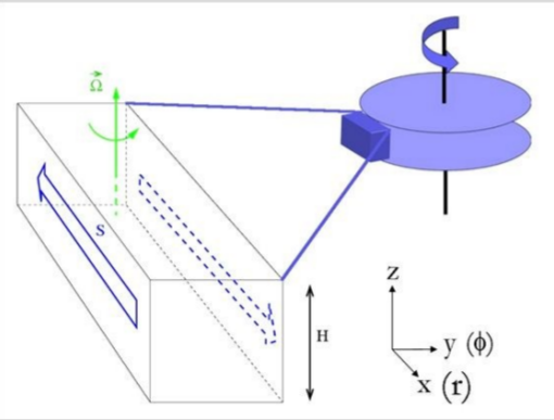
Figure 1: Model picture of local cubical box in accretion disk where we perform the analysis (http://ipag.obs.ujf-grenoble.fr/ longarep/astrophysics.html). Within the box, the Cartesian coordinate $x$ is along the radial cylindrical coordinate $r$ (with respect to the center of the accretion disk), $y$ is along $\phi$, and $z$ is same in both the systems.

To formulate the problem, we have considered a local box at a local patch in the accretion disk, as shown in the Fig. 1. Although the accretion disk possesses cylindrical geometry, In the local box, we study the motion of the local fluid element using the Cartesian coordinates. The one to one correspondence between the Cartesian ($x,y,z$) and cylindrical ($r,\phi,z$) coordinates are shown in the Fig. 1. The Cartesian coordinates $x,y,z$ are along the cylindrical coordinates $r,\phi,z$. The details of the local formulation are in Mukhopadhyay et al.[13, 14], and Ghosh and Mukhopadhyay[15]. As we confine ourselves in the local region of the accretion disks, the corresponding flow has been considered incompressible[16, 13, 17, 18, 9]. The governing equations are the ensemble-averaged Orr-Sommerfeld and Squire equations in the presence of Coriolis force and an additional stochastic force[19, 12], which is delta correlated with nonzero mean. The Orr-Sommerfeld and Squire equations are obtained by eliminating the pressure term from the corresponding Navier-Stokes equations and utilizing the continuity equation for the incompressible flow. The governing equations are given by,

$$\left(\frac{\partial}{\partial t}+U\frac{\partial}{\partial y}\right)\nabla^{2}u-U^{\prime\prime}\frac{\partial u}{\partial y}+\frac{2}{q}\frac{\partial\zeta}{\partial z}-\frac{1}{Re}\nabla^{4}u+\Gamma_{1}=NL^{u},$$ (1)

$$\left(\frac{\partial}{\partial t}+U\frac{\partial}{\partial y}\right)\zeta-U^{\prime}\frac{\partial u}{\partial z}-\frac{2}{q}\frac{\partial u}{\partial z}-\frac{1}{Re}\nabla^{2}\zeta+\Gamma_{2}=NL^{\zeta},$$ (2)

where $u$ and $\zeta$ are respectively the $x$-component of the velocity and vorticity perturbations after ensemble averaging, $U$ the $y$-component of background velocity which for the present purpose of plane shear in the dimensionless units is $-x$, $q$ the rotation parameter with $\Omega(r)\propto 1/r^{q}$, $\Omega(r)$ being the angular frequency of the fluid parcel at radius $r$, $\Gamma$-s are the corresponding constant means of stochastic forces (white noise with nonzero mean due to gravity making the system biased[11]) in the system described below, and $NL$-s are the non-linear terms due to the perturbation. The $x$-component of vorticity and the non-linear terms are given by

$$\zeta = \frac{\partial w}{\partial y}-\frac{\partial v}{\partial z},$$ (3)

$$NL^{u} = -\nabla^{2}\{(\textbf{u}^{\prime}\cdot\nabla)u\}+\frac{\partial}{\partial x}\nabla\cdot\{(\textbf{u}^{\prime}\cdot\nabla)\textbf{u}^{\prime}\},$$ (4)

$$NL^{\zeta} = -\frac{\partial}{\partial y}\{(\textbf{u}^{\prime}\cdot\nabla)w\}+\frac{\partial}{\partial z}\{(\textbf{u}^{\prime}\cdot\nabla)v\},$$ (5)

where $\textbf{u}^{\prime}=(u,v,w)$, which is the perturbed velocity vector. For the complete description of the flow, equations 1 and 2 are supplemented with the equation of continuity, which is given by

$$\nabla\cdot\textbf{u}^{\prime}=0,$$ (6)

To solve the governing equations, we have no-slip boundary conditions along $x$- direction [20, 13, 12], i.e. $u=v=w=0$ at $x=\pm 1$ or equivalently

$$u=\frac{\partial u}{\partial x}=\zeta=0,\,\ {\rm at}\,\,x=\pm 1.$$ (7)

2.1 Linear Theory

In the evolution of linear perturbation, let the linear solutions be

$$u=\hat{u}(x,t)e^{i\textbf{k}\cdot\textbf{r}},$$ (8)

$$\zeta=\hat{\zeta}(x,t)e^{i\textbf{k}\cdot\textbf{r}},$$ (9)

with $\textbf{k}=(0,k_{y},k_{z})\ {\rm and}\ \textbf{r}=(0,y,z).$ Substitute these in equations (1) and (2), neglecting non-linear terms, we obtain

$$\begin{split}\frac{\partial}{\partial t}Q+i\mathcal{L}Q+\Gamma=0,\end{split}$$ (10)

where

$$\begin{split}Q=\begin{pmatrix}\hat{u}\\ \hat{\zeta}\end{pmatrix},\ \mathcal{L}=\begin{pmatrix}\mathcal{L}_{11}&\mathcal{L}_{12}\\ \mathcal{L}_{21}&\mathcal{L}_{22}\end{pmatrix},\ \mathcal{D}=\frac{\partial}{\partial x},\end{split}$$ (11)

$$\begin{split}\mathcal{L}_{11}=&(\mathcal{D}^{2}-k^{2})^{-1}\Bigl{[}k_{y}U\left(\mathcal{D}^{2}-k^{2}\right)-k_{y}U^{\prime\prime}-\frac{1}{iRe}\left(\mathcal{D}^{2}-k^{2}\right)^{2}\Bigr{]},\\ \mathcal{L}_{12}=&\left(\mathcal{D}^{2}-k^{2}\right)^{-1}\frac{2k_{z}}{q},\\ \mathcal{L}_{21}=&-\left(U^{\prime}+\frac{2}{q}\right)k_{z},\\ \mathcal{L}_{22}=&k_{y}U-\frac{1}{iRe}\left(\mathcal{D}^{2}-k^{2}\right),\end{split}$$

and

$$\Gamma=e^{-i\textbf{k}\cdot\textbf{r}}\begin{pmatrix}(\mathcal{D}^{2}-k^{2})^{-1}\Gamma_{1}\\ \Gamma_{2}\end{pmatrix}.$$ (12)

Let us subsequently assume the trial solution of the equation (10) be

$$Q=AQ_{x}e^{-i\sigma t}-\frac{1}{\mathcal{D}_{t}+i\mathcal{L}}\Gamma,$$ (13)

where $\sigma$ is the eigenvalue corresponding to the particular mode and it is complex having real ($\sigma_{r}$) and imaginary ($\sigma_{i}$) parts,

$$Q_{x}=\begin{pmatrix}\phi^{u}(x)\\ \phi^{\zeta}(x)\end{pmatrix}$$ (14)

and $\mathcal{D}_{t}$ stands for ${\partial}/{\partial t}.$ $Q_{x}$ is the eigenfunction corresponding to the homogeneous part of the equation (10), i.e., $Q_{x}$ satisfies $\mathcal{L}Q_{x}=\sigma Q_{x}$. The first term of the right-hand side of the equation (13) is due to the homogeneous part of the equation (10), and the second term is due to the inhomogeneous part, i.e., the presence of $\Gamma$, of the same equation. Hence, $Q$ is influenced by the force $\Gamma$. However, the typical eigenspectra for the Keplerian flow ($q=1.5$), constant angular momentum flow ($q=2$) and plane Couette flow ($q\rightarrow\infty$) for $Re=2000$ and $k_{y}=k_{z}=1$ are shown in the Fig. 2. Since $\mathcal{L}_{12}$ and $\mathcal{L}_{21}$ in the equation (11) are zero for the plane Couette flow and constant angular momentum flow, respectively, we obtain the same eigenspectra for both plane Couette, and constant angular momentum flows. We perform the whole analysis for the least stable modes for the respective flows, and these least stable modes are shown in the dotted box in Fig. 2.

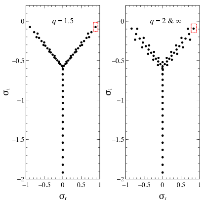
Figure 2: Variation of $\sigma_{i}$ with $\sigma_{r}$ for $Re=2000$ and $k_{y}=k_{z}=1$ for the Keplerian flow ($q=1.5$), constant angular momentum flow ($q=2$) and plane Couette flow ($q\rightarrow\infty$). The latter two eigenspectra are identical. The dotted box represents the least stable mode for the respective cases.

2.2 Nonlinear theory

For the non-linear solution, following similar work but in the absence of force [20, 21, 22], we assume the series solution for velocity and vorticity, i.e.

$$\psi=\sum_{n\rightarrow-\infty}^{\infty}\psi_{n}=\sum_{n\rightarrow-\infty}^{\infty}\bar{\psi}_{n}(t,x)e^{in(\textbf{k}\cdot\textbf{r}-\sigma_{r}t)},$$ (15)

when obviously $\bar{\psi}_{-n}=\bar{\psi}^{*}_{n}$ and $\psi$ could be any one of $u$ and $\zeta$.

We substitute these in equations (1) and (2) and collect the coefficients of the term $e^{i(\textbf{k}\cdot\textbf{r}-\sigma_{r}t)}$, to capture least nonlinear effect following, e.g., [20, 22, 12], from both sides and obtain

$$\frac{\partial Q_{1}}{\partial t}-i\sigma_{r}Q_{1}+i\mathcal{L}Q_{1}=NL_{1},$$ (16)

where $NL_{1}=\begin{pmatrix}\left(\mathcal{D}^{2}-k^{2}\right)^{-1}NL^{u}_{1}\\ NL^{\zeta}_{1}\end{pmatrix}$ and $Q_{1}=\begin{pmatrix}\bar{u}_{1}(x,t)\\ \bar{\zeta}_{1}(x,t)\end{pmatrix}$. We assume the solution for $Q_{1}$ to be

$$Q_{1}=\sum_{m=1}^{\infty}{A_{t,m}}{Q_{x,m}}-\frac{1}{\mathcal{D}_{t}+i\mathcal{L}}\Gamma,$$ (17)

where $m$ stands for various eigenmodes.

However, to the first approximation, our interest is in the least stable mode. Similar descriptions in two dimensions [20] without $\Gamma$ and three-dimensional Keplerian disks[22] without $\Gamma$ are already there in the in the literature and we mostly follow their formalism. We, therefore, omit the summation, and subscript $m$ in the equation (17), and obtain

$$Q_{1}={A_{t}}{Q_{x}}-\frac{1}{\mathcal{D}_{t}+i\mathcal{L}}\Gamma.$$ (18)

We then substitute the equation (18) in the equation (16) and using bi-orthonormality between $Q_{x}$ and its conjugate function $\tilde{Q}_{x}$, we obtain

$$\frac{dA_{t}}{dt}-\sigma_{i}A_{t}+\mathcal{N}=p|A_{t}|^{2}A_{t},$$ (19)

where

$$\mathcal{N}=\int_{-1}^{1}{dx\tilde{Q}_{x}^{\dagger}\Gamma^{\prime}}$$ (20)

and

$$p=\int_{-1}^{1}{dx\tilde{Q}_{x}^{\dagger}\mathcal{S}},$$ (21)

where

$$\begin{split}\Gamma^{\prime}=&-\Gamma+i\sigma_{r}\Bigl{(}\frac{1}{\mathcal{D}_{t}+i\mathcal{L}}\Bigr{)}\Gamma&\\ &=-\Gamma+i\sigma_{r}(t-i\mathcal{L}t^{2})(1+\mathcal{L}^{2}t^{2})^{-1}\Gamma,&\end{split}$$ (22)

$\mathcal{S}$ is the spatial contribution from the nonlinear terms. For the greater details, see Ghosh and Mukhopadhyay[12].

Throughout the paper, $\Gamma$ from the equation (12) has been decomposed as $\Gamma\rightarrow\Gamma\begin{pmatrix}1\\ 1\end{pmatrix}$ by adjusting $\Gamma_{1}$ and $\Gamma_{2}$, as they are only the free parameters.

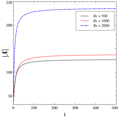
Figure 3: Variation of $\mathcal{N}$ as a function of $t$ for $Re=500,\ 1000$ and 2000, for $\Gamma=10^{4}$ and $k_{y}=k_{z}=1$, corresponding to the respective least stable modes.

The evolution of $\mathcal{N}$ has been shown in Fig. 3 for the parameters mentioned in the figure. It shows that $\mathcal{N}$ becomes saturated beyond a certain time, and the saturation depends on $Re$. As $Re$ increases, the saturation increases.

Figure 4: Variation of the least stable $\sigma_{i}$ as a function of $Re$ for $k_{y}=k_{z}=1$ in the Keplerian flow.

Fig. 4 shows the variation of the least stable (the one in the dotted box in Fig. 2) as a function of $Re$ in the case of the Keplerian flow. It tells us that the least stable mode approaches zero as $Re$ is increased.

3 Results

Equation (19), which is a nonlinear equation, tells us about the evolution of the amplitude of the perturbation. To explore the evolution of linear and nonlinear perturbations, we use the equation (19) accordingly. For the evolution of the linear perturbation, we get rid of the nonlinear term in equation (19).

3.1 Evolution of $|A|_{t}$ in the linear regime

In the linear regime, the equation (19) becomes

$$\frac{dA_{t}}{dt}=\sigma_{i}A_{t}-\mathcal{N}.$$ (23)

This equation tells that at large $t$, $|A_{t}|$ becomes $|\mathcal{N}|/|\sigma_{i}|$[12].

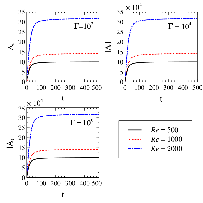
Figure 5: Variation of $|A_{t}|$ as a function of $t$ for three sets of $Re$ and $\Gamma$ with $k_{y}=k_{z}=1$ for linear analysis in the Keplerian flow ($q=1.5$).

Fig. 5 shows the variation of $|A_{t}|$ as a function of $t$ for various values of $Re$ and $\Gamma$. Fig. 5 also suggests the scaling relation between saturated $|A_{t}|$ and $\Gamma$ to be

$$|A_{t}|\propto\Gamma$$ (24)

for a fixed $Re$. Apart from that, we notice that for a fixed $\Gamma$, $|A|_{t}$ becomes saturated at $|\mathcal{N}|/|\sigma_{i}|$ beyond a certain time, and the saturation increases as $Re$ increases. This saturation is independent of the initial condition[12]. This is because at a fixed $\Gamma$, $|\mathcal{N}|$ becomes saturated (see Fig. 3) at a fixed value, and the saturated value increases as $Re$ increases, as well as $|\sigma_{i}|$ increases as $Re$ increases (see Fig. 4). Now, in the accretion disk, $Re$ is huge[19] ($\gtrsim 10^{14}$). The smaller $\Gamma$, therefore, can bring nonlinearity in the accretion disk, as for huge $Re$, $|\sigma_{i}|$ is infinitesimally small. Hence, $|\mathcal{N}|/|\sigma_{i}|$ becomes enormous. This huge saturation of $|A_{t}|$ could bring nonlinearity and hence plausibly turbulence in the underlying Keplerian flow.

3.2 Evolution of $|A_{t}|$ in the nonlinear regime

In the nonlinear regime, the evolution of $|A_{t}|$ is described by the equation (19). Fig. 6 describes the variation of $|A_{t}|$ as a function of $t$ for nonlinear perturbation in the Keplerian flow. In the figure, $RE(A_{t})$ and $IM(A_{t})$ indicate the real and imaginary parts of initial $A_{t}$, respectively. It tells us that for $\Gamma=0$, depending on the initial amplitude, $|A_{t}|$ may diverge (green line) or $|A_{t}|$ may decay (continuous black line) to zero from the initial amplitude. When there is no noise, i.e., $\Gamma=0$, the diverging solution of $|A_{t}|$ occurs when the initial amplitude is beyond a critical amplitude[12]. It is apparent that the onset of the nonlinearity depends on the initial amplitude of perturbation in the absence of the force, but it does not depend on the same in the presence of force[12]. The divergence of $|A_{t}|$ and hence the onset of nonlinearity and plausible turbulence depends only on the strength of the force, as shown by dashed (magenta) line, compared to dot-dashed (blue) and dotted (red) lines, in Fig. 6.

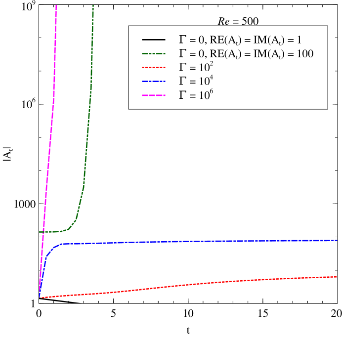
Figure 6: Variation of $|A_{t}|$ as a function of $t$ with $k_{y}=k_{z}=1$ for nonlinear analysis in the Keplerian flow for $Re=500$ and four different $\Gamma$. For $\Gamma\neq 0$, initial condition is RE($A_{t}$) = IM($A_{t}$) = 1.

4 Conclusion

If there is no extra force involved in the system, then the equation (19) becomes the usual Landau equation, which is

$$\frac{dA_{t}}{dt}=\sigma_{i}A_{t}+p|A_{t}|^{2}A_{t},$$ (25)

which can be further recast to

$$\frac{d|A|^{2}}{dt}=k_{1}|A|^{2}+k_{2}|A|^{4},$$ (26)

where $A$ is the amplitude of the nonlinear perturbations for the corresponding system, $k_{1}$ is 2$\sigma_{i}$ and $k_{2}$ is the real part of $2p$, i.e., 2$p_{r}$. Its solution is

$$|A|^{2}=\frac{A_{0}^{2}}{-\frac{k_{2}}{k_{1}}A_{0}^{2}+\left(1+\frac{k_{2}}{k_{1}}A_{0}^{2}\right)e^{-k_{1}t}},$$ (27)

where $A_{0}$ is the initial amplitude. Depending on the sign (positive/negative) of $k_{1}$ and $k_{2}$, there are four[23, 21] different possible evolutions of $|A|$. These given below.

• In the present context of shear flows, $k_{1}$ (i.e., $\sigma_{i}$) is negative, but $k_{2}$ is positive. Therefore, there will be a threshold for initial amplitude $A_{i}$, determining the growth of perturbation. If the initial amplitude $A_{0}<A_{i}$, then

  $$|A|^{2}\sim\frac{A_{i}^{2}A_{0}^{2}e^{k_{1}t}}{A_{i}^{2}-A_{0}^{2}}$$ (28)

  at a large $t$. Therefore, $|A|^{2}\rightarrow 0$ for $A_{0}<A_{i}$ at $t\rightarrow\infty$. However, if $A_{0}>A_{i}$, then $|A|^{2}\rightarrow\infty$ at $t\rightarrow\ln(1-A_{i}^{2}/A_{0}^{2})/k_{1}$.

• If both $k_{1}$ and $k_{2}$ would be positive, $|A|^{2}$ blows up after a finite time. Hence, there will be a fast transition to turbulence.

• On the other hand, if $k_{1}>0$ but $k_{2}<0$, then $|A|^{2}\rightarrow k_{1}/|k_{2}|$ at $t\rightarrow\infty$. In this case, $|A|^{2}$ at a large $t$ does not depend on $A_{0}$.

• Obviously, for $k_{1}$ and $k_{2}$ both negative, $|A|^{2}$ decays fast.

However, we have shown that the saturation in $|A_{t}|$ is $|\mathcal{N}|/|\sigma_{i}|$ in the linear regime. We have also argued that depending on $Re$ and $\Gamma$, the system may already be in the nonlinear regime. The evolution of $|A_{t}|$ at the linear regime in our case, i.e., with extra force, is similar to that of $|A|$ from the equation (26), i.e. without force, for $k_{1}>0$ and $k_{2}<0$. In the Keplerian flow, $k_{1}$, i.e. $\sigma_{i}$, is negative, but $k_{2}$, i.e. $p_{r}$, could be positive. In the presence of extra force, the Landau equation modifies in such a way that the solution in the linear regime itself mimics the Landau equation without force (i.e., equation 26), however, with $k_{1}>0$ and $k_{2}<0$. Further, in the nonlinear regime, the amplitude $A_{t}$ (i.e., with extra force included) diverges beyond a certain time, depending on $Re$ and $\Gamma$. In the nonlinear regime, the Landau equation in the presence of extra force but negative $k_{1}$ ($\sigma_{i}$) is, therefore, mimicking the Landau equation without force but with positive $k_{1}$ and $k_{2}$. Essentially, the extra force effectively changes the sign of $k_{1}$ (i.e., $\sigma_{i}$) for the Landau equation without force. Speaking in another way, the very presence of extra force destabilizes the otherwise stable system. Thus, the presence of force plays an important role in developing nonlinearity and turbulence in the case of Rayleigh stable flows.

References

- [1] N. I. Shakura and R. A. Sunyaev, Black holes in binary systems. Observational appearance, Astronomy & Astrophysics 24, 337 (1973).
- [2] D. Lynden-Bell and J. E. Pringle, The Evolution of Viscous Discs and the Origin of the Nebular Variables, Monthly Notices of the Royal Astronomical Society 168, 603 (09 1974).
- [3] S. A. Balbus and J. F. Hawley, A powerful local shear instability in weakly magnetized disks. I - Linear analysis. II - Nonlinear evolution, The Astrophysical Journal 376, 214 (July 1991).
- [4] E. Velikhov, Stability of an ideally conducting liquid flowing between rotating cylinders in a magnetic field, Zhur. Eksptl’. i Teoret. Fiz. 36 (05 1959).
- [5] S. Chandrasekhar, The Stability of Non-Dissipative Couette Flow in Hydromagnetics, Proceedings of the National Academy of Science 46, 253 (February 1960).
- [6] X.-N. Bai, Wind-driven Accretion in Protoplanetary Disks. II. Radial Dependence and Global Picture, The Astrophysical Journal 772, p. 96 (Aug 2013).
- [7] M. E. Pessah and D. Psaltis, The Stability of Magnetized Rotating Plasmas with Superthermal Fields, The Astrophysical Journal 628, 879 (August 2005).
- [8] U. Das, M. C. Begelman and G. Lesur, Instability in strongly magnetized accretion discs: A global perspective, Monthly Notices of the Royal Astronomical Society 473, 2791 (2018).
- [9] S. K. Nath and B. Mukhopadhyay, Origin of nonlinearity and plausible turbulence by hydromagnetic transient growth in accretion disks: Faster growth rate than magnetorotational instability, Physical Review E 92, p. 023005 (August 2015).
- [10] T. Singh Bhatia and B. Mukhopadhyay, Exploring non-normality in magnetohydrodynamic rotating shear flows: Application to astrophysical accretion disks, Physical Review Fluids 1, p. 063101 (October 2016).
- [11] S. K. Nath and B. Mukhopadhyay, A Pure Hydrodynamic Instability in Shear Flows and Its Application to Astrophysical Accretion Disks, The Astrophysical Journal 830, p. 86 (October 2016).
- [12] S. Ghosh and B. Mukhopadhyay, Hydrodynamical instability with noise in the Keplerian accretion discs: modified Landau equation, Monthly Notices of the Royal Astronomical Society 496, 4191 (August 2020).
- [13] B. Mukhopadhyay, N. Afshordi and R. Narayan, Bypass to Turbulence in Hydrodynamic Accretion Disks: An Eigenvalue Approach, The Astrophysical Journal 629, 383 (August 2005).
- [14] B. Mukhopadhyay, R. Mathew and S. Raha, Growing pseudo-eigenmodes and positive logarithmic norms in rotating shear flows, New Journal of Physics 13, p. 023029 (February 2011).
- [15] S. Ghosh and B. Mukhopadhyay, Forced linear shear flows with rotation: rotating couette-poiseuille flow, its stability and astrophysical implications (2021).
- [16] Yecko, P. A., Accretion disk instability revisited - transient dynamics of rotating shear flow, Astronomy & Astrophysics 425, 385 (2004).
- [17] N. Afshordi, B. Mukhopadhyay and R. Narayan, Bypass to Turbulence in Hydrodynamic Accretion: Lagrangian Analysis of Energy Growth, The Astrophysical Journal 629, 373 (August 2005).
- [18] F. Rincon, G. I. Ogilvie and C. Cossu, On self-sustaining processes in Rayleigh-stable rotating plane Couette flows and subcritical transition to turbulence in accretion disks, Astronomy & Astrophysics 463, 817 (Mar 2007).
- [19] B. Mukhopadhyay and A. K. Chattopadhyay, Stochastically driven instability in rotating shear flows, Journal of Physics A Mathematical General 46, p. 035501 (January 2013).
- [20] T. Ellingsen, B. Gjevik and E. Palm, On the non-linear stability of plane Couette flow, Journal of Fluid Mechanics 40, 97 (1970).
- [21] P. Schmid, D. Henningson and D. Jankowski, Stability and Transition in Shear Flows. Applied Mathematical Sciences, Applied Mechanics Reviews 55, p. B57 (2002).
- [22] S. R. Rajesh, Weakly non-linear stability of a hydrodynamic accretion disc, Monthly Notices of the Royal Astronomical Society 414, 691 (June 2011).
- [23] P. G. Drazin and W. H. Reid, Hydrodynamic Stability September 2004.