Galaxy shapes of Light (GaLight): a 2D modeling of galaxy images

Abstract

galight is a Python-based open-source package that can be used to perform two-dimensional model fitting of optical and near-infrared images to characterize the light distribution of galaxies with components including a disk, bulge, bar, and quasar. The decomposition of stellar components has been demonstrated in published studies of inactive galaxies and quasar host galaxies observed by the Hubble Space Telescope and Subaru’s Hyper Suprime-Cam. galight utilizes the image modeling capabilities of lenstronomy while redesigning the user interface for the analysis of large samples of extragalactic sources. The package is user-friendly with some automatic features such as determining the cutout size of the modeling frame, searching for PSF-stars in field-of-view, estimating the noise map of the data, identifying all the objects to set the initial model and associated parameters to fit them simultaneously. These features minimize the manpower and allow the automatic fitting tasks. The software is distributed under the MIT license. The source code, installation guidelines, and example notebooks code can be found at https://galight.readthedocs.io/en/latest/.

1 Introduction

Accurate surface photometry and morphology of galaxies are key to understanding the evolution of galaxies. Over the past few decades, the light distribution of galaxies has been successfully studied using analytic functions to estimate their size, luminosity, concentration, orientation and symmetry. Of all tested analytic models, the Sérsic model function [1] is the most successful and commonly used, which provides an accurate description of the surface brightness of galaxies, ranging from exponential disks (i.e., late-type galaxies) to de Vaucouleurs’s profiles [2] for describing early-type galaxies. The success of these analytic functions further allow us to analyze the light of a unique type of object, i.e., active galactic nuclei (AGN), which has been recognized to play an important role in the evolution galaxies and the growth of its central supermassive black hole (SMBH). While a central AGN can be bright, even above that of its host galaxy, we can still infer the photometry and morphology of the underline host galaxy based on the use of analytic models and deblending techniques.

With current and upcoming large imaging surveys, the sample of galaxies with quality imaging is growing rapidly and will continue to do so with future facilities. Thus, there is a great demand to process such large numbers of galaxy images in an automated manner with efficiency and accuracy.

Here, we present a first public release of galight, an open source python software package to model galaxy images including those hosting AGN. galight uses routines available through lenstronomy [3, 4] that are further described below. galight adds a number of features to process large numbers of images from survey data. This tool has been used to model the galaxy images from Hubble Space Telescope (HST) [5, 6] and Subaru Hyper Suprime-Cam (HSC) [7, 8], including a sample of $\sim$1.5 million galaxies and $\sim$5 thousand quasars profiting from the automatic features.

While other packages, such as Galfit [9] and GIMD2D [10], have provided the community much needed capabilities for analyzing galaxy images, there are benefits available with lenstronomy which we aim to fully exploit. For example, the parameter estimation is based on a forward modeling approach with semi-linear inversion of the amplitude components using machinery that includes a particle swarm optimizer (PSO) [11, 12] and Markov Chain Monte Carlo (MCMC) error analysis by emcee [13]. The ability to account for uncertainties on the point spread function (PSF) is also an important feature. Equally important, lenstronomy – an astropy-affiliated python tool for gravitational lensing image simulations and analyses – is an open source software package that can be easily installed and adapted to the user’s modeling needs due to its flexibility.

While functions provided by lenstronomy are suitable to model the light distribution of a galaxy, some additional work is needed to define the models, set the initial parameters and priors, implement masks for nearby objects, and assess specific requirements for each image cutout. As described here, the software package galight can set all the necessary parameters and perform automatic modeling with much needed efficiency, particularly for the analysis of large samples. Below, we introduce the basic functions of galight and demonstrate its capabilities.

The paper is organized as follows. In Section 2 and 3, we present a brief overview of the package which is structured in three major classes. In Section 4, we provide detailed information with some example code and figures. We highlight features in the Appendix and a summary is given in Section 5. We refer the reader to a number of studies that have made use of galight [5, 6, 7, 8].

2 Package overview

galight is open source python-based [14] software with distribution granted through the MIT open source software license. The software relies on the python standard library and the open-source libraries including numpy [15], scipy [16], astropy [17, 18], matplotlib [19] and photutils [20]. In particular, the package lenstronomy [3, 4] is the work horse that performs the fitting process. galight is compatible with both python 2 and python 3. However, the latter version is recommended.

The public release version of galight is on Pypi and can be installed using pip:

⬇

$ pip install galight --user

We also distribute galight on GitHub, while more stable versions released through Pypi. Documentation is available through sphinx and released on ReadtheDocs. To fully demonstrate the usage of this package, we provide several Jupyter notebooks with extended features.

galight helps the user to execute model fitting with ease based on, but not limited to, automated features as listed as follows:

1. Determining a suitable cutout size for the image frame. The cutout should have a minimal size that balances the need to reduce computing time and capture the extend of low surface brightness emission. The cutout will also keep neighboring galaxies away from the edge of the frame. This enables these galaxies to be properly modeled which may have outer light profiles that overlap with the central target of interest.

2. The PSF model is key for image (de-)convolution and accounting for an unresolved point source component (i.e., AGN and small unresolved components). The common practice is to manually select a star in the field of view (FOV) for characterizing the PSF. galight will search for all the PSF-stars in the FOV, report their full width at half maximum (FWHM), and allow the user to choose those suitable for determining the empirical PSF model.

3. If needed, a noise map can be generated based on the exposure time and the background noise level measured from empty regions.

4. Neighboring sources can be simultaneously modeled or easily be masked out.

5. By default, all the objects in the modeling frame will be detected by the photutils.detect_sources. Based on the detection results, the parameter settings for all these sources will be assigned automatically.

6. Output data products are generated for full assessment of the goodness-of-fit with the ability to share across different computing platforms.

In practice, galight is able to perform the fitting tasking without manual supervision after the target position and the modeling materials are provided.

3 Model-fitting procedure

galight uses three steps to achieve a successful modeling of image data. Here, we provide a brief overview of each step as defined by one python class and provide further details in Section 4.

1. DataProcess: The data products are prepared including the cutout of the science image, noise map, PSF model, and nearby object masks (optional). The image pixel scale and magnitude zero point should also be provided to galight to calculate physical quantities (i.e., target magnitudes and galaxy size in arcsec).

2. FittingSpecify: The model components (e.g., single Sérsic profile, disk$+$bulge, AGN, etc.) and associated parameters should be defined by this class. For example, the initial values and priors of the parameters are assigned. Priors can be given as either a range for each parameter with uniform or weighted sampling, or a single fixed value.

3. FittingProcess: The model fitting is performed, and the results are presented in this step. The user can determine the method of parameter inference (e.g., minimization and MCMC). Once the fitting has completed, this class provides the modeling output for diagnostic and demonstration purposes.

3.1 Analytical model and fitting strategies

Through lenstronomy, the model components are defined and the fitting is performed. The imported features include the definition of the light profile and the approach to sampling the parameter space.

Light profiles: All extended light profiles defined by lenstronomy are imported and available. These include, but not limited to, Sérsic [1], Chameleon [21], ellipsoid, 2D Gaussian, pseudo Jaffe [22], Moffat [23], and power-law functions. We refer the reader to the lenstronomy documentation for further details.

By default, the Sérsic profile [1] is adopted to describe the light of extended object with parameterization as follows:

$$I(R)=A\exp\left[-k\left(\left(\frac{R}{R_{\mathrm{eff}}}\right)^{1/n}-1\right)\right],$$ (1)

$$R(x,y,q)=\sqrt{x^{2}+y^{2}/q^{2}},$$ (2)

where $A$ is the amplitude and $q$ denotes the axis ratio. The Sérsic index $n$ controls the shape of the radial surface brightness profile, a larger $n$ corresponds to a steeper inner profile and a highly extended outer wing. $k$ is a constant which solely depends on $n$ to ensure that the isophote at $R=R_{\mathrm{eff}}$ encloses half of the total light [24]. Note that this definition of Sérsic profile is the same as the one adopted by Galfit in which the $R_{\mathrm{eff}}$ is the semi-major-axis half-light radius. The other definition of elliptical light profile with a format as $R(x,y,q)=\sqrt{qx^{2}+y^{2}/q}$ is also available in lenstronomy after version 1.9.0, hence galight. Both formats will be available to the user; however, note that the $R_{\mathrm{eff}}$ will be different by a factor of $\sqrt{q}$ between these two definitions.

We note that the light profile for spheroidal galaxies can usually be fitted with a single Sérsic profile and a free index $n$. In cases where more components are required, a composite light model can be implemented, such as a spheroid plus disk component (Sérsic $n$ = 1) and even a bar (Sérsic $n$ = 0.5).

When modeling the point-source flux component, such as an AGN component or star, a scaled PSF model will be adopted to characterize the unresolved emission. The amplitude and the position of the point source will be considered as free parameters. As demonstrated in next section, a PSF model can be directly input to galight. Alternatively, galight can search for suitable stars over the full image to generate an empirical PSF model. To account for an imperfect model PSF, one can also provide an uncertainty on the PSF which will be considered when calculating the likelihood and best-fit model parameters. Taking the PSF model uncertainty into account can be important, especially when estimating the uncertainty of the fitting parameters. This is likely an important feature of galight which is not a feature directly implemented in the currently most commonly used modeling codes. To note, the PSF model is also used for the convolution of the total emission in the forward-modeling.

Fitting algorithm: To obtain the inference of the best-fit parameters, a likelihood is calculated by lenstronomy using the lenstronomy.ImSim module while sampling of the parameter space is performed by the lenstronomy.Sampling module. Briefly, a likelihood estimator is implemented to determine the values of the posterior distribution based on the data and model $p(d_{\rm data}|d_{\rm model})$ (i.e., the probability of the data given a model) using all the counted pixels in the full cutout which can be presented as follows:

$$\log p(d_{\text{data}}|d_{\text{model}})=\sum_{i}\frac{(d_{\text{data,i}}-d_{\text{model,i}})^{2}}{2\sigma_{\text{i}}^{2}}+C.$$ (3)

The errors (i.e., $\sigma_{\text{i}}$) are assigned based on the noise map. For fitting, the noise map can be directly input to galight. If not provided, the tool can calculate the total noise map according to the following two terms:

$$\sigma_{i}^{2}=\sigma_{\text{bkgd}}^{2}+|d_{\text{data,i}}/(t_{\rm exp}\times G_{\rm eff})|,$$ (4)

i.e., a Gaussian background term (i.e., $\sigma_{\text{bkg}}$), and a Poisson term, i.e., $\sqrt{|d_{\text{data,i}}/(t_{\rm exp}\times G_{\rm eff})|}$ , where $t_{\rm exp}$ is the exposure time (in seconds) of the observational data (given in counts per second) and $G_{\rm eff}$ is the effective gain values. By default, the Sérsic surface brightness amplitude (i.e., the parameter $A$ in Equation 1) is linear parameters that is solved directly during the likelihood estimation. This modeling strategy saves a type of non-linear parameter and would lead to better and faster convergence; even more, it can be generalized to more components and basis sets.

4 Learning to use galight through examples

We provide detailed descriptions of the routines and three core classes. In this paper, we give brief show-case examples and further demonstrations can be found online through Jupyter notebooks.

4.1 DataProcess

The following example in next page is a demonstration of the steps needed to prepare the class DataProcess. We provide example code (see next page) and highlight the relevant lines being discussed.

⬇

1import astropy.io.fits as pyfits

2#Load the data, noise map, PSF and header information based on astropy#

3dataFile = pyfits.open(’../example_data.fits’)

4fov_image = dataFile[1].data

5header = dataFile[1].header

6noiseFile = pyfits.open(’../example_noise.fits’)

7noise_map = noiseFile[1].data

8

9#Prepare for the fitting#

10from galight.data_process import DataProcess

11pos_RA, pos_Dec = 500, 500 #Assuming the target is at pixel position 500, 500#

12zp = 27.0 #Assuming the zeropoint of the detection is 27.0#

13rm_bkglight = True #The background light will be modeled and removed as a 2D profile by photutils.background.SExtractorBackground() .#

14

15#Input the information to DataProcess.#

16data_process = DataProcess(fov_image = fov_image, target_pos = [pos_RA, pos_Dec], fov_noise_map = noise_map, header = header, rm_bkglight = rm_bkglight, zp = zp)

17

18#Preparing fitting ingredients, including cutout image, noise map and masks (if needed).#

19data_process.generate_target_materials(radius=65, create_mask = True, nsigma=2.8, exp_sz= 1.2, npixels = 15)

20#Automatically find all the PSF-stars and select the best one to use for fitting.#

21data_process.find_PSF(radius = 30, user_option = True)

22#Alternatively, the users can load a PSF model manually through:#

23#data_process.PSF_list = [PSF]#

24

25#Check out if all the fitting ingredients are ready. If not, an error message will appear.#

26data_process.checkout()

galight retrieves the pixel scale from the image header (line 16), or this is set by the user manually data_process.deltaPix. The location of the target can be given as either a pixel position or with ‘WCS’ information as RA and DEC (line 11). The function generate_target_materials (line 19) extracts a square region centered on the target and creates an image stamp having a frame size of $(2\times$radius$+1)$. If the radius value is assigned as ‘None’, galight will determine a minimum value, ranging from 30 to 70 pixels, that avoids having nearby objects not fully covered by the cutout image. Of course, for nearby galaxies, the upper boundary might not be sufficient and the user should select their own value.

Objects in the frame are detected as part of the generate_target_materials function, and characterized by a set of elliptical apertures as shown in Figure 1 (left and middle panels). The user is given the option to either mask any object or model them simultaneously in the fitting procedure (see notebook entitled  ‘galight_HST_QSO.ipynb’ for more details). As shown in the figure, the object #0 is our fitting target which is assigned by aperture #0. The other nearby objects are also assigned by the corresponding apertures. These apertures are saved in ‘data_process.apertures’, and by default they reveal how the data will be fitted as a sets of elliptical Sérsic profiles; the properties of these apertures (including positions, size, ellipticity and orientation) will be used to assign the initial parameters of the Sérsic profiles to model. One can manually change the properties of apertures in this step to modify the initials that will be used in the fitting. The user can also add the apertures manually to increase the number of Sérsic profiles that to be fitted. For example, if we aim to fitting our targeting galaxy as disk$+$bulge, we can creat a smaller aperture (i.e., a bulge component) and add it to the position at the aperture #0. The python notebook  ‘galight_HSC_galaxy.ipynb’ demonstrates how this setting can be achieved. The prior settings for the Sérsic profiles are introduced in next section. In addition, these apertures can be used to assign the masks to block the pixels for any object in the fitting. In this example, we mask out the object #1 in the fitting as shown in the Figure.

For this example, the noise level of the data is known and directly loaded (see line 16, the noise_map, in the example code). If this information is not provided, the generate_target_materials function will automatically measure the background noise level from empty regions and combine this with the Poisson noise component. We demonstrate the estimation of the noise map in A.

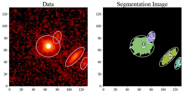
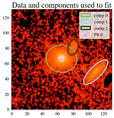
Figure 1: Example target with HST cutout images. Left panel: Detected objects in the cutout frame are highlighted by white elliptical apertures. middle panel: Each object is labeled with individual numbers to help the user to select those to be masked. right panel: After user input, the final settings show how this image will be modeled. All apertures indicate the initial settings to fit the extended sources. ‘PS0’ marks the center of the fitted point source of interest. Here, object #1 has been masked out thus filled in black in the bottom right panel.

A model PSF is required for the convolution and, if needed, as an individual component to represent an unresolved point source. If the PSF model is available with an image, it can be input to the DataProcess() class directly (see line 23 in the example code). Alternatively, a PSF can be constructed based on stars in the field-of-view of the science image. We provide a functionality to search for PSF stars across the entire image in data_process.find_PSF(). The user can then select the preferred objects based on the sharpness of their light profile or for any other reason. A demonstration of how to search for suitable objects to generate an empirical model PSF is provided in B. Online notebooks (  ‘find_PSF_in_FOV.ipynb’ and  ‘galight_HST_QSO.ipynb’) demonstrate this feature. To assign an error on the PSF, one can define an array type that has the same dimensions as the PSF (see next section).

4.2 FittingSpecify

In this class, the light model and parameters are set. Since the aim of galight is to automatize the process, there are very few steps required for the user. An example is as follows.

⬇

1#Produce the class and params to make the QSO decomposition.#

2from galight.fitting_specify import FittingSpecify

3

4#Pass the data_process to FittingSpecify#

5fit_sepc = FittingSpecify(data_process)

6

7#Prepare the fitting sequence, point_source_num defines the number of point source (i.e., AGN) that to fit.#

8fit_sepc.prepare_fitting_seq(point_source_num = 1)

9

10#Plot the initial settings for fittings. #

11fit_sepc.plot_fitting_sets()

12

13#Build up all the settings and get prepared to pass to the next class.#

14fit_sepc.build_fitting_seq()

The apertures determined by DataProcess() in previous step are applied and the initial Sérsic parameters are set as starting points for the fitting. The main settings of the fit routine are controlled by prepare_fitting_seq() which take arguments that can be set as follows:

1. point_source_num sets the number of point sources needed for the fit (default = 0). This should be set to one for a quasar or a star. By default, the software will automatically find the source with brightest peak in the cutout frame and use the peak position as the initial position to perform the fit.

2. fix_center_list sets the priors on the position so that an AGN and its host galaxy are fixed to the same central position.

3. fix_n_list can be assigned to fix the Sérsic index value and fix_Re_list can be assigned to fix the Sérsic R_eff value.

4. psf_error_map defines the PSF error map with the same dimensions as the input PSF. The values of the error map are added at the fitted point source position to the final noise map as:
   $\sigma_{i}^{2}=\sigma_{i}^{2}$ + psf_error_map${}_{j}*($point_source_flux$)^{2}$.

Examples of these setting can be found in the online notebooks. Detailed information is given in the online documentation through ReadtheDocs.

The prepare_fitting_seq() is designed to help the user quickly build up the requisites for the fitting using the templates embedded in the function. After this step, the user can make modifications to these settings to add complexity and make the fitting more sophisticated. For example, the FittingSpecify.kwargs_params is a dictionary that saves all the parameters settings for the Sérsic model and the point sources including the initials, sampling steps, fixed value, lower and upper limit. The user can change the corresponding values therein to modify the lower and upper limits for any parameters so that these parameters will be limited in the desired range and sampled with a flat prior. Additional priors can also be added to the likelihood. For example, defining the disk size to be larger than the bulge size or any arbitrary prior on the parameters (e.g., a Gaussian prior), can be assigned through the FittingSpecify.kwargs_likelihood. These are demonstrated in  ‘galight_HSC_galaxy.ipynb’. Note that all this settings are in the format that defined by lenstronomy; the user should follow its guidance to achieve more sophisticated fittings.

Finally, the user can use plot_fitting_sets() to display how the target and nearby sources will be modeled as shown here in the right panel of Figure 1.

4.3 FittingProcess

The fitting routine is executed after FittingSpecify has been passed to FittingProcess:

⬇

1#Setting the fitting method and run:#

2from galight.fitting_process import FittingProcess

3#Pass fit_sepc to FittingProcess:#

4fit_run = FittingProcess(fit_sepc, savename = ’savename’)

5#Setting the fitting approach and run. The fitting process will be save as ’savename.pkl’#

6fit_run.run(algorithm_list = [’PSO’, ’MCMC’], setting_list = [None, None]))

By default, the procedure first performs the minimization of the parameters using the particle swarm optimizer ( [PSO, 11, 12]) algorithm and then passes the inferred minimized parameters to the MCMC routine (e.g., emcee [13]) to estimate their best-fit values and uncertainties. In the FittingProcess.run(), i.e., line 6 in the example, the user can re-define the algorithm_list to increase the times of minimization or skip the MCMC through the arguments. Moreover, the sampling parameters such as the fitting particles and the number of iterations can be defined through setting_list.

Once parameter estimation has finished, the trace of the PSO and MCMC fitting chains will be plotted to help the user diagnose the convergence of the fitting routine.

⬇

1#Fitting has done. Now, plot the fitting results (as shown in Figure 2, top panel):#

2fit_run.plot_final_qso_fit()

3#Calculate the physical properties, such as magnitude, for each component:#

4fit_run.translate_result()

5#Plot the MCMC inference of the flux for each component (as Figure 2, bottom panel):#

6fit_run.plot_flux_corner()

The MCMC parameter inferences are translated to fluxes values and displayed in the bottom panel of Figure 2 with the posteriors on the flux of the individual components.

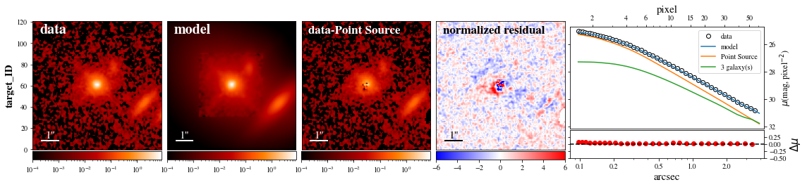
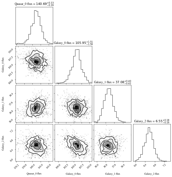
Figure 2: $top~{}panels$: Example modeling results of the image data shown in Figure 1. The panels from the left to right are: (1) observed science data, (2) best-fit model. The clear box around the galaxy reveals the region of the PSF size that used to model the AGN. (3) data - point-source model (i.e., host galaxy only) (4) residuals divided by variance (i.e., reduced $\chi^{2}$ map), (5) surface brightness profiles in 1D (top) and the residual (bottom). $Bottom~{}panels$: the MCMC inference of the likelihood distribution of the fitted parameters are translated to flux values (i.e., the total pixel counts) for each fitted component. The labels for each component correspond to those in the right panel of Figure 1. Note that the flux values are not the parameters that fitted directly.

5 Conclusion

We present an open-source python-based tool –galight– to decompose galaxies into their various components. The software is distributed under the MIT license. Taking advantage of many of the functionalities of lenstronomy, the modeling is composed of three steps, separated into individual classes. We briefly introduce the functions of each class and present the example results in Section 4. galight provides additional functions to setup the fitting routine and complete the modeling in an automated manner. Our aim is to minimize intervention by the user so that large data sets can be processed seamlessly.

The demonstrations and other features mentioned in this paper are included in example notebooks in https://github.com/dartoon/galight_notebooks as listed here.

1. ‘galight_HST_QSO.ipynb’: Modeling example of an HST observed quasar image. In this example, the PSF is reconstructed by a PSF-star in the FOV and the noise map is calculated using galight based on the approach introduced in A.

2. ‘galight_HSC_QSO.ipynb’: Modeling example of an HSC imaged quasar, in which the PSF and noise map are supplied to galight.

3. ‘galight_HSC_dualAGN.ipynb’: Modeling example of an HSC imaged double AGN candidate.

4. ‘galight_HSC_galaxy.ipynb’: Modeling example of an HSC imaged galaxy. As demonstration, the galaxy is modeled as composite model with disk and bulge components.

These online resources will be updated periodically.

Citing the code: This manuscript is posted on arXiv as a user manual, which will be constantly updated in the future with more upcoming features. We ask the users of galight please make reference to Ding et al., ApJ, 2020, 888, 37 and lenstronomy [4] when use it.

6 Acknowledgements

This software is supported by World Premier International Research Center Initiative (WPI), MEXT, Japan.

Appendix A Noise map estimation

If user does not provide an error map, galight will calculate the noise level for each pixel which is composed of a Gaussian background noise and Poisson noise components, (see Equation 4). First, galight detects all objects and then masks them to identify the empty (sky) regions to measure the average signal. We demonstrate an example of this measurement in Figure 3. A Gaussian formalization is used to measure the standard derivation. Since the background light has been subtracted by setting rm_bkglight = True in DataProcess(), the median of the distribution should close to zero, which can be easily checked (Figure 3; right panel). The Poisson noise is estimated based on the pixel number counts and the exposure time, where exposure time can be input as either a single value or a array map. Alternatively, the user can measure the Gaussian background themselves and directly input the error map to galight.

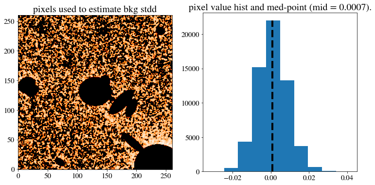
Figure 3: left: Measuring the background noise level with galight. The emission from the objects in the field are detected and masked so that the sky pixels can be identified. right: Histogram of the number counts from sky pixels. The black dashed line is the median value. Since the background light has been removed in our example, the position of the median value is located at zero.

Appendix B Search for PSF-stars in the image FOV

galight can search for available PSF-stars in the FOV of the image using function DataProcess.findPSF. The algorithm is designed so that it looks for the local maximum pixel with prominent features (like PSF), achieved by the function scipy.ndimage.filters. During this search process, the code measures the FWHM values of each PSF candidates and discards those with extended profiles. Moreover, PSF-stars that are too faint or bright, compared with the target will be removed by default.

We demonstrate the search of PSF stars in the FOV. The FWHM and 1D profile is also presented to the user to aid in the selection of the best PSF to use for the fitting (see Figures 4, 5 and 6). By default, the PSF with the sharpest profile (i.e., the one with smallest FWHM value) will be selected.

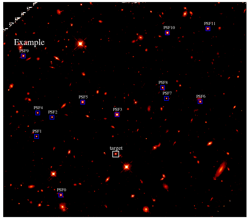
Figure 4: Identifying suitable PSF stars in a HST/WFC3 field. Candidates found by galight are marked by small blue boxes and checked as to whether they are not too bright or too faint.

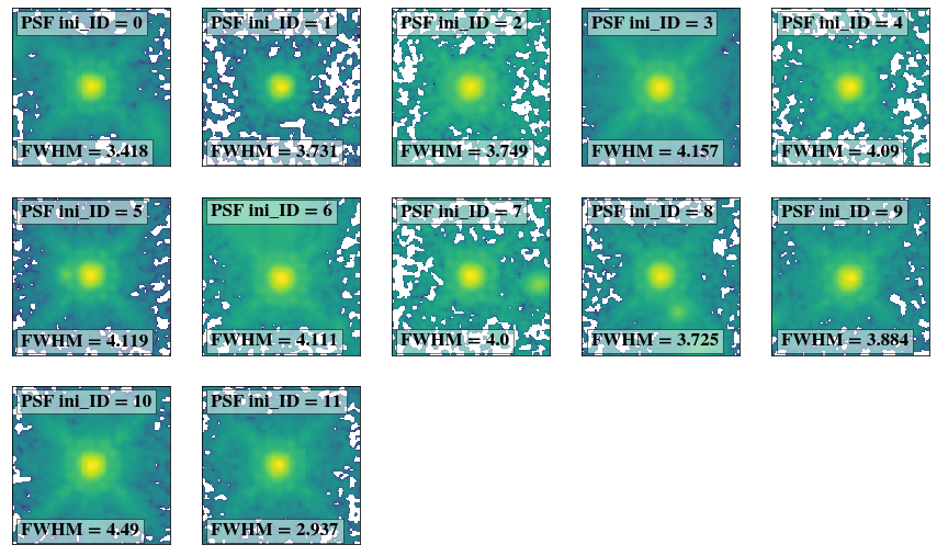
Figure 5: Zoom-in images of the PSF model candidates. During this process, the FWHM (in units of pixel scales) of each PSF is measured and reported to help the user select the best PSFs for their application.

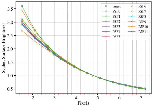
Figure 6: The 1D surface brightness profile of each PSF model candidates compared to the targets.

References

- [1] J. L. Sersic, Atlas de Galaxias Australes, 1968.
- [2] G. de Vaucouleurs, Recherches sur les Nebuleuses Extragalactiques, Annales d’Astrophysique 11 (1948) 247.
- [3] S. Birrer, A. Amara, lenstronomy: Multi-purpose gravitational lens modelling software package, Physics of the Dark Universe 22 (2018) 189–201. arXiv:1803.09746, doi:10.1016/j.dark.2018.11.002.
- [4] S. Birrer, A. Shajib, D. Gilman, A. Galan, J. Aalbers, M. Millon, R. Morgan, G. Pagano, J. Park, L. Teodori, N. Tessore, M. Ueland, L. Van de Vyvere, S. Wagner-Carena, E. Wempe, L. Yang, X. Ding, T. Schmidt, D. Sluse, M. Zhang, A. Amara, lenstronomy II: A gravitational lensing software ecosystem, The Journal of Open Source Software 6 (62) (2021) 3283. arXiv:2106.05976, doi:10.21105/joss.03283.
- [5] X. Ding, J. Silverman, T. Treu, A. Schulze, M. Schramm, S. Birrer, D. Park, K. Jahnke, V. N. Bennert, J. S. Kartaltepe, A. M. Koekemoer, M. A. Malkan, D. Sanders, The Mass Relations between Supermassive Black Holes and Their Host Galaxies at 1 ¡ z ¡ 2 HST-WFC3, ApJ 888 (1) (2020) 37. arXiv:1910.11875, doi:10.3847/1538-4357/ab5b90.
- [6] V. N. Bennert, T. Treu, X. Ding, I. Stomberg, S. Birrer, T. Snyder, M. A. Malkan, A. W. Stephens, M. W. Auger, A local baseline of the black hole mass scaling relations for active galaxies. IV. Correlations between and host galaxy , stellar mass, and luminosity, arXiv e-prints (2021) arXiv:2101.10355arXiv:2101.10355.
- [7] S. Tang, J. D. Silverman, X. Ding, J. Li, K.-G. Lee, M. A. Strauss, A. Goulding, M. Schramm, L. Kawinwanichakij, J. X. Prochaska, J. F. Hennawi, M. Imanishi, K. Iwasawa, Y. Toba, I. Kayo, M. Oguri, Y. Matsuoka, K. Ichikawa, T. Hartwig, N. Kashikawa, T. Kawaguchi, K. Kohno, Y. Matsuda, T. Nagao, Y. Ono, M. Onoue, M. Ouchi, K. Shimasaku, H. Suh, N. Suzuki, Y. Taniguchi, Y. Ueda, N. Yasuda, Optical Spectroscopy of Dual Quasar Candidates from the Subaru HSC-SSP program, arXiv e-prints (2021) arXiv:2105.10163arXiv:2105.10163.
- [8] J. Li, J. D. Silverman, X. Ding, M. A. Strauss, A. Goulding, S. Birrer, H. M. Yesuf, Y. Xue, L. Kawinwanichakij, Y. Matsuoka, Y. Toba, T. Nagao, M. Schramm, K. Inayoshi, The Sizes of Quasar Host Galaxies with the Hyper Suprime-Cam Subaru Strategic Program, arXiv e-prints (2021) arXiv:2105.06568arXiv:2105.06568.
- [9] C. Y. Peng, L. C. Ho, C. D. Impey, H.-W. Rix, Detailed Structural Decomposition of Galaxy Images, AJ 124 (1) (2002) 266–293. arXiv:astro-ph/0204182, doi:10.1086/340952.
- [10] L. Simard, GIM2D: an IRAF package for the Quantitative Morphology Analysis of Distant Galaxies, in: R. Albrecht, R. N. Hook, H. A. Bushouse (Eds.), Astronomical Data Analysis Software and Systems VII, Vol. 145 of Astronomical Society of the Pacific Conference Series, 1998, p. 108.
- [11] J. Kennedy, R. Eberhart, Particle swarm optimization, in: Proceedings of ICNN’95 - International Conference on Neural Networks, Vol. 4, 1995, pp. 1942–1948 vol.4. doi:10.1109/ICNN.1995.488968.
- [12] S. Birrer, A. Amara, A. Refregier, Gravitational Lens Modeling with Basis Sets, ApJ 813 (2) (2015) 102. arXiv:1504.07629, doi:10.1088/0004-637X/813/2/102.
- [13] D. Foreman-Mackey, D. W. Hogg, D. Lang, J. Goodman, emcee: The MCMC Hammer, PASP 125 (925) (2013) 306. arXiv:1202.3665, doi:10.1086/670067.
- [14] G. Van Rossum, F. L. Drake Jr, Python reference manual, Centrum voor Wiskunde en Informatica Amsterdam, 1995.
-
[15]
C. R. Harris, K. J. Millman, S. J. van der Walt, R. Gommers, P. Virtanen,
D. Cournapeau, E. Wieser, J. Taylor, S. Berg, N. J. Smith, R. Kern, M. Picus,
S. Hoyer, M. H. van Kerkwijk, M. Brett, A. Haldane, J. F. del Río,
M. Wiebe, P. Peterson, P. Gérard-Marchant, K. Sheppard, T. Reddy,
W. Weckesser, H. Abbasi, C. Gohlke, T. E. Oliphant,
Array programming with
NumPy, Nature 585 (7825) (2020) 357–362.
doi:10.1038/s41586-020-2649-2.
URL https://doi.org/10.1038/s41586-020-2649-2 - [16] P. Virtanen, R. Gommers, T. E. Oliphant, M. Haberland, T. Reddy, D. Cournapeau, E. Burovski, P. Peterson, W. Weckesser, J. Bright, S. J. van der Walt, M. Brett, J. Wilson, K. J. Millman, N. Mayorov, A. R. J. Nelson, E. Jones, R. Kern, E. Larson, C. J. Carey, İ. Polat, Y. Feng, E. W. Moore, J. VanderPlas, D. Laxalde, J. Perktold, R. Cimrman, I. Henriksen, E. A. Quintero, C. R. Harris, A. M. Archibald, A. H. Ribeiro, F. Pedregosa, P. van Mulbregt, SciPy 1.0 Contributors, SciPy 1.0: Fundamental Algorithms for Scientific Computing in Python, Nature Methods 17 (2020) 261–272. doi:10.1038/s41592-019-0686-2.
- [17] Astropy Collaboration, T. P. Robitaille, E. J. Tollerud, P. Greenfield, M. Droettboom, E. Bray, T. Aldcroft, M. Davis, A. Ginsburg, A. M. Price-Whelan, W. E. Kerzendorf, A. Conley, N. Crighton, K. Barbary, D. Muna, H. Ferguson, F. Grollier, M. M. Parikh, P. H. Nair, H. M. Unther, C. Deil, J. Woillez, S. Conseil, R. Kramer, J. E. H. Turner, L. Singer, R. Fox, B. A. Weaver, V. Zabalza, Z. I. Edwards, K. Azalee Bostroem, D. J. Burke, A. R. Casey, S. M. Crawford, N. Dencheva, J. Ely, T. Jenness, K. Labrie, P. L. Lim, F. Pierfederici, A. Pontzen, A. Ptak, B. Refsdal, M. Servillat, O. Streicher, Astropy: A community Python package for astronomy, A&A 558 (2013) A33. arXiv:1307.6212, doi:10.1051/0004-6361/201322068.
- [18] Astropy Collaboration, A. M. Price-Whelan, B. M. Sipőcz, H. M. Günther, P. L. Lim, S. M. Crawford, S. Conseil, D. L. Shupe, M. W. Craig, N. Dencheva, A. Ginsburg, J. T. VanderPlas, L. D. Bradley, D. Pérez-Suárez, M. de Val-Borro, T. L. Aldcroft, K. L. Cruz, T. P. Robitaille, E. J. Tollerud, C. Ardelean, T. Babej, Y. P. Bach, M. Bachetti, A. V. Bakanov, S. P. Bamford, G. Barentsen, P. Barmby, A. Baumbach, K. L. Berry, F. Biscani, M. Boquien, K. A. Bostroem, L. G. Bouma, G. B. Brammer, E. M. Bray, H. Breytenbach, H. Buddelmeijer, D. J. Burke, G. Calderone, J. L. Cano Rodríguez, M. Cara, J. V. M. Cardoso, S. Cheedella, Y. Copin, L. Corrales, D. Crichton, D. D’Avella, C. Deil, É. Depagne, J. P. Dietrich, A. Donath, M. Droettboom, N. Earl, T. Erben, S. Fabbro, L. A. Ferreira, T. Finethy, R. T. Fox, L. H. Garrison, S. L. J. Gibbons, D. A. Goldstein, R. Gommers, J. P. Greco, P. Greenfield, A. M. Groener, F. Grollier, A. Hagen, P. Hirst, D. Homeier, A. J. Horton, G. Hosseinzadeh, L. Hu, J. S. Hunkeler, Ž. Ivezić, A. Jain, T. Jenness, G. Kanarek, S. Kendrew, N. S. Kern, W. E. Kerzendorf, A. Khvalko, J. King, D. Kirkby, A. M. Kulkarni, A. Kumar, A. Lee, D. Lenz, S. P. Littlefair, Z. Ma, D. M. Macleod, M. Mastropietro, C. McCully, S. Montagnac, B. M. Morris, M. Mueller, S. J. Mumford, D. Muna, N. A. Murphy, S. Nelson, G. H. Nguyen, J. P. Ninan, M. Nöthe, S. Ogaz, S. Oh, J. K. Parejko, N. Parley, S. Pascual, R. Patil, A. A. Patil, A. L. Plunkett, J. X. Prochaska, T. Rastogi, V. Reddy Janga, J. Sabater, P. Sakurikar, M. Seifert, L. E. Sherbert, H. Sherwood-Taylor, A. Y. Shih, J. Sick, M. T. Silbiger, S. Singanamalla, L. P. Singer, P. H. Sladen, K. A. Sooley, S. Sornarajah, O. Streicher, P. Teuben, S. W. Thomas, G. R. Tremblay, J. E. H. Turner, V. Terrón, M. H. van Kerkwijk, A. de la Vega, L. L. Watkins, B. A. Weaver, J. B. Whitmore, J. Woillez, V. Zabalza, Astropy Contributors, The Astropy Project: Building an Open-science Project and Status of the v2.0 Core Package, AJ 156 (3) (2018) 123. arXiv:1801.02634, doi:10.3847/1538-3881/aabc4f.
- [19] J. D. Hunter, Matplotlib: A 2d graphics environment, Computing in Science & Engineering 9 (3) (2007) 90–95. doi:10.1109/MCSE.2007.55.
-
[20]
L. Bradley, B. Sipőcz, T. Robitaille, E. Tollerud, Z. Vinícius,
C. Deil, K. Barbary, T. J. Wilson, I. Busko, H. M. Günther, M. Cara,
S. Conseil, A. Bostroem, M. Droettboom, E. M. Bray, L. A. Bratholm, P. L.
Lim, G. Barentsen, M. Craig, S. Pascual, G. Perren, J. Greco, A. Donath,
M. de Val-Borro, W. Kerzendorf, Y. P. Bach, B. A. Weaver, F. D’Eugenio,
H. Souchereau, L. Ferreira,
astropy/photutils: 1.0.0 (Sep.
2020).
doi:10.5281/zenodo.4044744.
URL https://doi.org/10.5281/zenodo.4044744 - [21] A. A. Dutton, B. J. Brewer, P. J. Marshall, M. W. Auger, T. Treu, D. C. Koo, A. S. Bolton, B. P. Holden, L. V. E. Koopmans, The SWELLS survey - II. Breaking the disc-halo degeneracy in the spiral galaxy gravitational lens SDSS J2141-0001, MNRAS 417 (3) (2011) 1621–1642. arXiv:1101.1622, doi:10.1111/j.1365-2966.2011.18706.x.
- [22] Á. Elíasdóttir, M. Limousin, J. Richard, J. Hjorth, J.-P. Kneib, P. Natarajan, K. Pedersen, E. Jullo, D. Paraficz, Where is the matter in the Merging Cluster Abell 2218?, arXiv e-prints (2007) arXiv:0710.5636arXiv:0710.5636.
- [23] A. F. J. Moffat, A Theoretical Investigation of Focal Stellar Images in the Photographic Emulsion and Application to Photographic Photometry, A&A 3 (1969) 455.
- [24] L. Ciotti, G. Bertin, Analytical properties of the R1/m law, A&A 352 (1999) 447–451. arXiv:astro-ph/9911078.