MASCOT - An ESO-ARO legacy survey of molecular gas in nearby SDSS-MaNGA galaxies: I. first data release, and global and resolved relations between H₂ and stellar content

Abstract

We present the first data release of the MaNGA-ARO Survey of CO Targets (MASCOT), an ESO Public Spectroscopic Survey conducted at the Arizona Radio Observatory (ARO). We measure the CO(1-0) line emission in a sample of 187 nearby galaxies selected from the Mapping Nearby Galaxies at Apache Point Observatory (MaNGA) survey that has obtained integral field unit (IFU) spectroscopy for a sample of $\sim$ 10,000 galaxies at low redshift. The main goal of MASCOT is to probe the molecular gas content of star-forming galaxies with stellar masses $>10^{9.5}$ M_⊙ and with associated MaNGA IFU observations and well-constrained quantities like stellar masses, star formation rates and metallicities. In this paper we present the first results of the MASCOT survey, providing integrated CO(1-0) measurements that cover several effective radii of the galaxy and present CO luminosities, CO kinematics, and estimated H₂ gas masses. We observe that the decline of galaxy star formation rate with respect to the star formation main sequence (SFMS) increases with the decrease of molecular gas and with a reduced star formation efficiency, in agreement with results of other integrated studies. Relating the molecular gas mass fractions with the slope of the stellar age gradients inferred from the MaNGA observations, we find that galaxies with lower molecular gas mass fractions tend to show older stellar populations close to the galactic center, while the opposite is true for galaxies with higher molecular gas mass fractions, providing tentative evidence for inside-out quenching.

1 Introduction

Understanding the behaviour of the cold phase of the interstellar medium (ISM) is central to understanding the galaxy evolution process as a whole. Galaxies exist in a state of flux, being subject to a range of physical processes (including accretion, gas outflow, and star formation) which are the drivers of their evolution (Tumlinson et al., 2017; Péroux & Howk, 2020). For example, star formation is regulated by the amount of available gas and internal feedback processes (Kennicutt, 1998b; Harrison, 2017; Rupke, 2018). The tight relation between molecular gas and star formation has been studied for decades (Sanders & Mirabel, 1985; Solomon et al., 1997; Combes et al., 2007; Young et al., 2011; Saintonge et al., 2011, 2017; Lin et al., 2019b; Colombo et al., 2020), and has come to represent a central pillar of our understanding of galaxy evolution as well as a critical ingredient in models (Bouché et al., 2010; Lilly et al., 2013; Saintonge et al., 2016). However, disentangling the detailed physics underlying this correlation remains an important area of research. As such, attaining a better understanding of the gas content of galaxies, in particular the molecular gas content, which is the fuel for star formation, is key to understanding how galaxies evolve.

Carbon Monoxide, ¹²C¹⁶O, is the most widely used tracer of molecular gas, both in the local and in the high-$z$ Universe. The luminosities of the low-$J$ CO transitions, in particular the lowest energy CO($1-0$) emission line (rest frequency $\nu=115.271$ GHz), can be used to measure the mass of molecular gas, modulo a conversion factor $\rm{\alpha_{CO}}$ (for a review, see Bolatto et al., 2013). Several large surveys have therefore targeted the low-$J$ transitions of CO to measure the probe gas content in the past decade. The COLD GASS survey (CO Legacy Database for GASS; Saintonge et al., 2011) used the IRAM 30m telescope to measure the CO(1-0) line in a sample of $\sim$350 nearby (D=100-200 Mpc), massive galaxies with $\log(M_{*}/M_{\odot})>10.0$ selected from the Sloan Digital Sky Survey (SDSS). The survey was later expanded to also include lower-mass galaxies (xCOLDGASS; Saintonge et al., 2017), bringing the combined surveys to a sample size of 532 galaxies probing the entire star formation rate (SFR) - stellar mass plane above $\log(M_{*}/M_{\odot})>9.0$. Furthermore, the ALLSMOG survey (APEX low-redshift legacy survey for molecular gas; Bothwell et al., 2014; Cicone et al., 2017) complements the xCOLDGASS survey by providing CO(2-1) emission line observations of 88 nearby, low-mass ($8.5<\log(M_{*}/M_{\odot})<10$) galaxies taken with the APEX-1 receiver on the APEX telescope. These surveys revealed that it is both the molecular gas mass fraction, i.e. the molecular gas to stellar mass ratio $f_{\rm{H_{2}}}=M_{H_{2}}/M_{*}$, as well as the star formation efficiency (SFE = SFR / M${}_{H_{2}}$) that vary strongly as a function of specific star formation rate and determine a galaxy’s offset from the star forming main sequence. The CO luminosity appears to correlate not only strongly with stellar mass and SFR but also varies with metallicity and HI mass.

These surveys were able to explore the connection between the global gas content of galaxies where galaxy parameters had been obtained via single-fibre SDSS spectroscopy (and SDSS photometry). That means all information about stellar mass, star formation rate, central AGN activity, concentration parameter, metallicity was therefore restricted to a central 3$\arcsec$ aperture probing very different spatial scales depending on the redshift of the source. Integral field unit (IFU) surveys now offer new possibilities in investigating the spatial dimension of galaxy evolution and allow these quantities to be mapped in two dimensions (Cappellari et al., 2011; Sánchez et al., 2012; Croom et al., 2012; Bundy et al., 2015).

The SDSS-IV (Blanton et al., 2017) survey Mapping Nearby Galaxies at APO (MaNGA; Bundy et al., 2015; Drory et al., 2015; Law et al., 2015; Yan et al., 2016b, a; Wake et al., 2017) is an optical fibre-bundle IFU survey that has mapped the detailed composition and kinematic structure of 10,010 unique nearby galaxies at $0.01<z<0.15$. The current public data release, DR15 (Aguado et al., 2019b), includes data for 4824 MaNGA data cubes. The full MaNGA data set will be released as part of DR17, expected in December 2021. MaNGA delivers resolved optical spectroscopic data. Many critical diagnostics, which provide insight into the formation processes of galaxies, such as metallicity gradients, age gradients, and resolved AGN diagnostics, and are only available to such resolved observations. However, the cold, molecular gas phase is not probed by MaNGA observations.

We started to fill in this gap with the MaNGA Survey of CO Targets (MASCOT, Figure 1). MASCOT was initially granted 200 hours on the Arizona Radio Observatory (ARO) in 2018 to obtain molecular gas mass measurements of MaNGA galaxies via the ¹²CO(1-0) transition. After that first successful set of observations, MASCOT was granted another 1200 hours with the ARO. A large survey for molecular gas in galaxies with existing IFU data represents a uniquely powerful tool for addressing a host of science questions and opens new avenues for molecular gas studies by drawing targets from the current generation of SDSS surveys.

The MASCOT survey complements other recent spatially-resolved observational programs in the community. The EDGE (Extragalactic Database for Galaxy Evolution) survey targeted 177 infrared-bright CALIFA (the Calar Alto Integral Field Area survey) galaxies using the Combined Array for Millimeter-wave Astronomy (CARMA). The survey targeted the ¹²CO(1-0) line and its ¹³CO isotopologue providing spatially resolved CO maps with a resolution corresponding to size scales of 0.5-2 kpc matched to the CALIFA observations (Bolatto et al., 2017). The maps have a half-power field-of-view (FOV) with radius $\sim 50\arcsec$, covering the galaxies out to $\sim 2-3$ effective radii (R_eff). This dataset enables studies of the relationships between molecular gas and its kinematics, stellar mass, star formation rate, metallicity, and dust extinction on kpc scales (Utomo et al., 2017; Colombo et al., 2018; Leung et al., 2018; Levy et al., 2018; Dey et al., 2019; Levy et al., 2019; Barrera-Ballesteros et al., 2020, 2021). These observations are currently being complemented by ¹²CO(2-1) measurements of CALIFA galaxies using the APEX 12m sub-millimetre telescope (Güsten et al., 2006). Compared to MASCOT, the CALIFA-APEX observations target galaxies at lower redshift ($0.005<z<0.03$) and provide less coverage. The first set of combined CARMA and APEX observations of CALIFA galaxies comprises 472 sources (Colombo et al., 2020). The APEX CO(2-1) beam covers the galaxies roughly out to 1 R_eff. By dividing the sample into galaxies that are centrally quenched and star forming galaxies, first results suggest that once star formation has been significantly reduced due to the consumption of molecular gas, changes in the star formation efficiency are what drives a galaxy deeper into the red sequence.

On the other hand, the ALMaQUEST (ALMA-MaNGA QUEnching and STar formation) survey is a program with spatially-resolved 12CO(1-0) measurements obtained with the Atacama Large Millimeter Array (ALMA) for 46 galaxies from MaNGA DR15 (Lin et al., 2020). The aim of the ALMaQUEST survey is to investigate the dependence of star formation activity on the cold molecular gas content at kpc scales in nearby galaxies and targets not only main-sequence galaxies, but also starburst and green valley galaxies (Lin et al., 2019b; Ellison et al., 2020a, b; Lin et al., 2020; Ellison et al., 2021a, b). The survey spatially resolves the CO(1-0) line on scales matching the MaNGA resolution and its field-of-view is $\sim$ 50”, very similar to the MASCOT observations. The ALMaQUEST survey is very complementary to MASCOT and we include their spatially integrated CO measurements in this paper (for details, see Section 3.8). Together, the EDGE-CALIFA and ALMaQUEST surveys provide complementary strengths for studying gas and star formation with supporting optical IFU data on kpc-scales in the nearby Universe.

In this paper we present the first data release of the MASCOT survey of molecular gas mass measurements for 187 galaxies selected from the MaNGA survey. The paper is structured as follows: In Section 2 we summarise the available MaNGA data products and additional ancillary data for the galaxies. In Section 3 we present details on the MASCOT survey, including the sample selection, details on the observations with the ARO, data reduction and analysis. Section 4 investigates some first global and resolved relations between the molecular gas mass measurements and the MaNGA-derived galaxy properties and in Section 5 we conclude. For the derived quantities we assume a flat $\Lambda$CDM cosmology with H₀ = 70 km s^-1 Mpc^-1, $\Omega_{\rm{m}}$ =0.3, $\Omega_{\Lambda}$ =0.7. We furthermore use the redshifts published in the NASA Sloan Atlas catalog (NSA catalog, Blanton et al., 2011).

2 SDSS MaNGA

2.1 Survey Description

Mapping Nearby Galaxies at Apache Point Observatory (MaNGA) is a two-dimensional spectroscopic survey and is part of the Sloan Digital Sky Survey-IV (SDSS-IV). MaNGA (Yan et al., 2016a) uses the BOSS spectrographs (Gunn et al., 2006; Smee et al., 2013) with $R\sim 2000$ to take integral field unit (IFU) observations of each galaxy in the 3,600 – 10,000Å range. Fibers are arranged into hexagonal bundles. The bundles have sizes that range from 19 – 127 fibres, depending on the apparent size of the target galaxy (which corresponds to diameters ranging between 12″ to 32″). This leads to an average footprint of $400-500$ arcsec² per IFU. The fibres have a size of 2″ aperture (2.5″ separation between fibre centres), which corresponds to $\sim 2$ kpc at $z\sim 0.05$, although with dithering the effective sampling improves to $1.4$″(see also Wylezalek et al., 2018). The current data release DR15 (Aguado et al., 2019a) contains 4,688 MaNGA galaxies (including ancillary targets and $\sim$ 65 repeat observations). MaNGA has observed 10,010 galaxies at $z\la 0.15$ and with stellar masses $>10^{9}M_{\odot}$ and the entire data set will become public as part of DR17 (currently scheduled for December 2021).

2.2 MaNGA Data Products

The data is first fed through the MaNGA Data Reduction Pipeline (DRP) which produces sky-subtracted spectrophotometrically calibrated spectra and rectified three-dimensional data cubes (Wylezalek et al., 2018). These combine individual dithered observations (for details on MaNGA data reduction see Law et al., 2016) with a spatial pixel scale of 0.5 ″ pixel^-1. The median spatial resolution of the MaNGA data is 2.54 ″ FWHM while the median spectral resolution is $\sim 72$ km/s (Law et al., 2016, 2021).

The MaNGA Data Analysis Pipeline (DAP, Belfiore et al., 2019; Westfall et al., 2019) is a project-led software package and is used to analyse the data products produced by the MaNGA DRP. The analysis results of the DAP provide the collaboration and public with survey-level quantities, such as spectral indices, kinematics and emission-line properties for 21 different emission lines. To make these calculations, the DAP first fits the stellar continuum using the Penalized Pixel-Fitting method (pPXF, Cappellari & Emsellem, 2004; Cappellari, 2017) and then performs a second fitting stage for the emission lines which optimises simultaneously the continuum and the emission lines, which are added as templates in a pPXF call. For example, for DR15, the DAP provides spatially stacked spectra, stellar kinematics (V and $\sigma$) derived on a set of Voronoi-binned spectra, spaxel-based nebular emission-line properties including fluxes, equivalent widths, and kinematics (V and $\sigma$) and spectral indices from absorption-lines (e.g., H$\delta$) and bandhead (e.g., D4000) measurements.

In this paper, we also make use of the Value Added Catalog ‘MaNGA Pipe3D’ (Sanchez et al., 2017a) which is based on measurements performed with the Pipe3D pipeline (Sánchez et al., 2016). The pipeline is designed to fit the continuum with stellar population models and to measure the nebular emission lines of IFS data. The stellar population library uses the (Salpeter, 1955) initial mass function. The stellar mass is then obtained based on the best-fit stellar population model. The stellar-population model spectra are then subtracted from the original cube allowing the analysis of the ionised gas emission lines (Sánchez et al., 2016). For example, the star formation rate was derived by using the H$\alpha$ luminosities for all the spaxels with detected ionised gas following the conversion given by Kennicutt (1998a) as well as from the single stellar population (SSP) fits computing the amount of stellar mass formed in the last 32Myr . The Value Added Products include both a set of datacubes, containing spatially resolved stellar population properties, star formation histories, emission line fluxes and stellar absorption line indices derived using the Pipe3D pipeline, as well as a catalog with one entry per galaxy, comprising the integrated properties of those galaxies (e.g., stellar mass, star-formation rate), and the characteristic values (e.g., oxygen abundance at the effective radius, all including the associated uncertainties . In this paper we make use of the integrated stellar masses and SSP-based SFRs.

We also point out to the reader that a number of additional ‘Value Added Catalogs’ publicly released by the SDSS collaboration. These catalogs have been created by MaNGA collaborators and are distributed through the SDSS Science Archive Server. In particular, we point out the ‘HI-MaNGA Data Release 1’ catalog which presents the first catalog of HI (21 cm neutral hydrogen) follow-up for MaNGA galaxies (Masters et al., 2019).

In this work, we furthermore make use of Marvin, a tool specifically designed to visualise and analyse MaNGA data. It is developed and maintained by the MaNGA team. Among other tools, Marvin allows the user to access reduced MaNGA datacubes locally, remotely, or via a web interface, access and visualise data analysis products and perform powerful queries on data and metadata . Details about Marvin are described in Cherinka et al. (2019) and on the Marvin website.

3 MASCOT Sample and Observations

3.1 Survey Description

The MASCOT sample is being assembled over the course of two programs at the Arizona Radio Observatory (ARO) as part of the MASCOT 1.0 and MASCOT 2.0 programs (PI: Wylezalek). As part of the agreement for transferring ownership of the ALMA prototype antenna to the University of Arizona to install it on Kitt Peak as a telescope of the ARO, ESO distributed to its user community a total of 3600h of observing time on the ARO telescopes from 2015 to 2020 . It was decided that this time should be dedicated to large Public Surveys with an important legacy value. MASCOT was chosen to be one of these surveys.

The first part of the survey, MASCOT 1.0, was awarded 200 hours of observing time in 2018 and the survey targeted 34 sources selected from the MaNGA survey. For the sample selection, we used the then available Data Release 14 (DR14, Abolfathi et al., 2018) which contained 2778 galaxies at $0.01<z<0.15$ with a mean $z\sim 0.05$.

The second part of the survey, MASCOT 2.0, was awarded 1200 hours spread over four semesters in 2019 and 2020 (P103-P106). Due to the COVID-related shutdown of the telescope in 2020, the timeline of the execution of the observations has been significantly delayed. Sources have been selected from the current MaNGA data release DR15.

At the time of writing of this paper, observations for 153 sources have been completed as part of MASCOT 2.0, resulting in a total number of observed MASCOT targets of 187. The distribution of the observed objects on the sky and in redshift space are shown in Figure 1 and Figure 3, respectively.

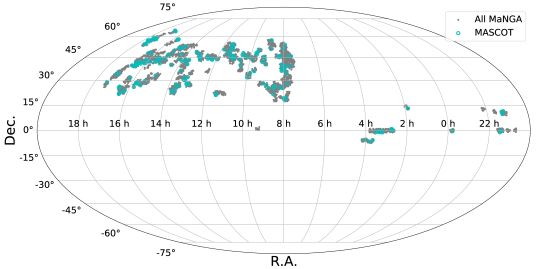
Figure 1: Sky distribution of observed MASCOT sources. We also show the distribution of the DR15 MaNGA sample as small grey points.

3.2 Sample Selection

The aim of this survey is to provide molecular gas measurements for galaxies with existing IFU data. All targets are therefore drawn from the sample of targets with existing observations from the MaNGA survey. The current MaNGA data release at the time of the start of the MASCOT 1.0 program in early 2018 consisted of $\sim$ 3000 members, but the survey continued to observe $\sim$ 1600 galaxies/year and public data releases happened on a yearly basis. As a result, the target list for MASCOT 2.0 has evolved and will continue to evolve over the remaining part of the survey, as MaNGA releases its complete and final data set (see Section 2.1).

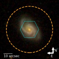
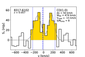
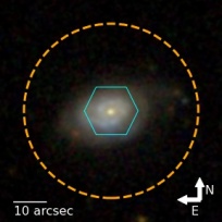
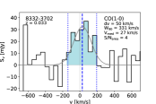
Figure 8: Left: SDSS three color image, also showing the MaNGA footprint (purple hexagon) and the ARO beam (orange dashed circle). Right: the MASCOT CO(1-0) line spectrum (solid black line). In cases where the spectrum was spectrally binned, the spectrum in native spectral resolution is shown in light grey. The final spectral resolution $dv$ is reported in the plot. When the CO(1-0) line is detected, the model fit is shown as the grey solid line and the line-of-sight velocity $v_{med}$ is indicated by the blue dashed line. Both $v_{05}$ and $v_{95}$, which are used for the $W_{90}$ determination, are indicated by the dotted blue lines. For sources detected at a S/N is $>5$, the part of the spectrum between $v_{05}$ and $v_{95}$ which is used for the data-based line flux measurement S_CO,data is coloured in yellow. For tentative detections with $3<$ S/N $<5$, that part is coloured in light blue.

We select our targets from MaNGA sources with available SFR measurements and we estimate the expected CO(1-0) luminosity from the total SFR by assuming the $SFR-L_{CO(1-0)}^{\prime}$ scaling relation obtained by Cicone et al. (2017, shown in Fig. 8 in their paper) for the ALLSMOG and COLDGASS samples of local star-forming galaxies (Saintonge et al., 2011; Cicone et al., 2017). We then derived the expected CO(1-0) integrated flux and the expected CO(1-0) peak flux density assuming a total line width of 200 km/s. These estimates were carried out to prioritise the first set of sources to be observed within MASCOT. Since we carried out observations spread over the entire year, our sample selection is independent of any R.A. constraints.

To test the (at that time unknown) telescope efficiency, in 2018, we chose to start the survey with the brightest sources with an expected CO(1-0) peak flux density $>75~{}mJy$, corresponding to a lower limit in molecular gas mass of $\log(M_{H_{2}}/M_{\odot})\sim 8.9$ for a galaxy with a redshift of $z=0.02$ (which corresponds to the mean redshift of our sample, see Figure 3). This selection ensured that we could either detect the CO(1-0) emission line in these targets at a $S/N>3$ or infer valuable upper limits on their molecular gas content. We integrated until the CO line is detected, or until we reached a 1-$\sigma_{\rm{rms}}$ sensitivity of 0.5 mK in $\delta v=50~{}km~{}s^{-1}$-wide channels, corresponding to $\sim 13$ mJy. That selection resulted in a sample of star forming galaxies located with a mean of $\sim$ 0.15 dex above the star formation main sequence.

The number of detections has exceeded our expectations given the previous estimates of the sensitivity of the receiver. Furthermore, the telescope has been upgraded with a new spectrometer (see Section 3.3) since the start of the MASCOT program in 2018. We have therefore adjusted our targeting strategy. To reduce the bias in selecting primarily star-forming galaxies, we have continued the survey drawing from the remaining MaNGA targets with an expected CO(1-0) peak flux density $>15$ mJy and adjusted our target 1-$\sigma_{\rm{rms}}$ sensitivity to 0.25 mK. In Figure 2 we show the distribution of the MASCOT sample in the SFR-M_∗ plane in comparison with the full MaNGA sample, where we use the stellar masses and SSP-derived SFR from the Pipe3D catalogue. The current sample of 187 galaxies is located with a median of $\sim$ 0.07 dex above the star formation main sequence.

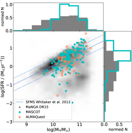
Figure 2: Distribution of the MASCOT targets in the SFR-M_∗ plane (cyan circles). We also show the distribution of the DR15 MaNGA sample (grey density map) and the distribution of targets from the complementary ALMAQuest sample (orange crosses). Additionally, we show the star formation main sequence (SFMS) as derived by Whitaker et al. (2012) and its associated scatter of $\pm 0.34$ dex (dashed lines). Most MASCOT sources lie above the SFMS owing to the selection process for this first part of the MASCOT survey. The ALMAQuest sources nicely complement the MASCOT sample in sampling sources on and below the SFMS. We also show the normalised distributions of the stellar masses M_∗ and SFR above and next to the main panel. For the normalisation, each bin displays the bin’s raw count divided by the total number of counts and the bin width.

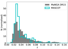
Figure 3: Normalised redshift distribution of the MASCOT sources in comparison to the MaNGA sample (DR15). For the normalisation, each bin displays the bin’s raw count divided by the total number of counts and the bin width.

3.3 Observations

Observations are carried out with the new 12m millimeter single dish telescope at the Arizona Radio Observatory. At the typical redshifts of the MaNGA sample ($z\sim 0.025$), the CO(1-0) line is conveniently redshifted to 112 GHz, where the atmospheric opacity is improved relative to 115 GHz. We used the 3mm receiver on the 12m ARO antenna (equivalent to ALMA Band 3, 84 – 116 GHz). The first part of the MASCOT survey (MASCOT 1.0) was carried out with the millimetre autocorrelator (MAC) backend on the ARO 12m antenna which provided a bandwidth of 800 MHz (600 MHz usable $\simeq$ 1600 km/s at 112 GHz). In August 2018, the new ARO Wideband Spectrometer (AROWS) backend was successfully commissioned on the 12m. AROWS offers an increased total bandwidth of 4000 MHz, sampling $>$ 5000 km/s around the CO(1-0) line and allowing for an improved baseline subtraction, especially for sources with broad CO(1-0) lines. The second part of the MASCOT survey (MASCOT 2.0) has been carried out with the AROWS backend and so will forthcoming observations. All observations are also still simultaneously recorded with the MAC, as a backup. Both the MAC and the AROWS give a velocity resolution of about $\sim~{}1$ km/s. Since our sources are ‘high velocity’ sources, i.e. galaxies with $z>0.02$, we tuned the telescope to the different rest frequencies and set that rest frequency to 0.0 km/s for all sources.

Observations are carried out in fixed observing blocks. The atmospheric conditions varied greatly, with a precipitable water vapor (PWV) ranging between 2 and 20 mm, with a mean of $\sim 5$ mm. Targets for this first data release were chosen and priorized based on their expected peak CO(1-0) flux density as described in Section 3.2 as well as on their observability. For example, we priorised targets with low ($<2$) airmass and avoided pointing towards the wind direction. We made ‘real-time’ decisions on the targets by performing on-the-fly data reductions of the observations, and observations were stopped once the target was detected at a significance of 5$\sigma$ or when we reached a root mean square ($\sigma_{\rm{rms}}$) of 0.5 mK (0.25 mK, see Section 3.2) per 50 km/s channel, corresponding to $\sim 13$ mJy ($\sim 7$ mJy), – which ever came first. In good observing conditions and for bright sources, conditions were met within one hour, but typical exposure times ranged between $\sim 2-3$ hours.

3.4 Data Reduction

The data are reduced with the CLASS software. All scans are visually examined and unusually noisy scans, scans with distorted baselines or anomalies are discarded. We then manually set a generous velocity window and estimate the baseline in each scan through a first-order fit to the continuum outside of that velocity window. If the CO line is undetected or very weak, we set the velocity window to [-300, 300] km/s. The scans are then averaged and saved as a fits file.

These spectra are still in units of the observed source antenna temperature corrected for atmospheric attenuation, radiative loss and rearward scattering and spillover $T_{R}^{*}$ . We therefore first convert to the main beam temperature $T_{mb}$ using $T_{mb}=T_{R}^{*}/\eta_{m}^{*}$, where $\eta_{m}^{*}$ is the corrected main beam efficiency. The flux density $f_{\nu}$ can then be derived from the Rayleigh-Jeans law such that

$$f_{\nu}=5.097\times 10^{-4}\frac{\rm{BWHM}^{2}}{\lambda^{2}}T_{mb}$$ (1)

where $f_{\nu}$ is in Jy, $\lambda$ is the observing wavelength in cm, and BWHM (beam width at half maximum) is the beam size in arcsec. The beam size at the frequency of our observations is 55 arcsec. The typical uncertainty in the main beam efficiency is $\sim 3-4$%.

3.5 Spectral Line Fitting

3.5.1 Dynamical spectral binning

We develop a customised spectral line fitting technique to measure the CO line fluxes and and kinematic parameters. We use the baseline subtracted averaged spectra in units of Jy as described in Section 3.4. Our aim is to dynamically bin the spectra depending on the measured signal-to-noise S/N at a given bin width $dv_{\rm{bin}}$. This procedure utilises non-parametric flux and velocity width measurements which are described in more detail in Section 3.5.2.

We begin by fitting a single Gaussian profile to the spectrum at its native spectral resolution (1–2 km/s depending on the redshift of the source) and allow the velocity offset $\Delta v$ to range between [-250, 250] km/s and the velocity dispersion to range between [50, 500] km/s. We then measure the cumulative flux

$$S(v)=\int_{-\infty}^{v}f_{v}(v^{\prime})dv^{\prime},$$ (2)

and the total line flux is given by $S(\infty)$. In practice, we use the interval [-3000, 3000] km s^-1 in the rest-frame of the galaxy for the integration.

We then determine $v_{05}$ such that $S(v_{05})=0.05\cdot S(\infty)$ and $v_{95}$ such that $S(v_{95})~{}=~{}0.95~{}\cdot~{}S(\infty)$. These are the velocities at which 5% and 95% of the total flux $S(\infty)$ are reached, respectively. We use these velocities to determine the width of the fitted line W₉₀ using W${}_{90}=v_{95}-v_{05}$. We measure the flux $S$ of the line from the data (i.e. not the Gaussian model) within W₉₀ and refer to it as S_CO,data (see Section 3.5.2). For the S_CO,data, we include the flux bins in which $v_{05}$ and $v_{95}$ fall.

We then determine the uncertainty $\epsilon$ on the flux by first determining the root-mean-square (rms) noise of the spectra. We measure the standard deviation of the noise per spectral channel, $\sigma_{\rm{rms}}$, outside the spectral window of [-250, 250] km/s (with respect to the 0 km/s rest frequency, see Section 3.3) and then compute

$$\epsilon=\frac{\sigma_{\rm{rms}}W_{90}}{\sqrt{N}},$$ (3)

where N is the number of channels within W₉₀, which can be determined by calculating W₉₀ / $dv_{\rm{bin}}$.

If the signal-to-noise ratio, $S/N=S(\infty)/\epsilon$, is determined to be $<20$, we spectrally bin the spectrum to a resolution of $dv_{\rm{bin}}$ = 10 km/s and repeat the described procedure. We repeat this process of increasing $dv_{\rm{bin}}$ in steps of 10 km/s until the line is measured with a S/N $>20$ or until we rebin the spectrum to a maximum $dv_{\rm{bin}}$ = 50 km/s. This procedure allows us to retain a better spectral sampling for the bright sources within our sample.

We provide the binned and unbinned spectra as part of the supplementary material to this paper, as well as on the MASCOT website.

3.5.2 CO Flux and CO Luminosity Measurements

Once the spectral binning (to a maximum of 50 km/s) has been optimised, we proceed with measuring the CO line flux. A single Gaussian is often insufficient for describing the profile of the CO(1-0) line. This is particularly true when secondary broad components characteristic of potentially outflowing gas or broad or double-peaked CO(1-0) emission in the case of rotating gas disks are contributing significantly to the emission line profile. To evaluate the prevalence of additional kinematic components, we therefore allow for two Gaussian components to be fitted to the CO line. The fitting procedure uses a least squares regression to return best-fit parameters for the single-Gaussian and double-Gaussian model. The $\chi^{2}$ value is then used to evaluate the goodness of the fit.

In cases where the spectral shape of an emission line is close to Gaussian, then the calculation of best fit parameters from a single Gaussian fit (i.e. velocity dispersion, full width at half maximum (FWHM), amplitude) are sufficient to describe its kinematic properties. This is not the case when multiple Gaussians are needed to describe the line profile (see also Wylezalek et al., 2020). We therefore calculate non-parametric values based on the percentages of the total integrated flux (see e.g. Liu et al., 2013). We compute the $S(v)$ based on the best-model fit (see equation 2 above). We then compute the line-of-sight velocity $v_{med}$ where $S(v_{med})=0.5\cdot S(\infty)$, i.e. this is the velocity that bisects the total area underneath the emission-line profile. Because the fitting is performed in the rest-frame of the galaxy as determined by its stellar component, $v_{med}$ is measured relative to the rest-frame (see also Wylezalek et al., 2020). We use the W₉₀ parameter to parameterise the velocity width of the CO line. W₉₀ refers to the velocity width that encloses 90% of the total flux. We determine $v_{05}$ and $v_{95}$ and then calculate W₉₀ using W${}_{90}=v_{95}-v_{05}$. The advantage of using W₉₀ over the Gaussian velocity dispersion is that it quasi independent of the underlying model used to fit the profile. We also compute W${}_{50}=v_{75}-v_{25}$ for easier comparison with other works and enhancing the legacy value of our work.

We then compute the CO(1-0) line flux in three different ways: $(i)$ by integrating the spectrum data within $v_{05}$ and $v_{95}$ yielding S_CO,data, $(ii)$ by integrating the model fit within $v_{05}$ and $v_{95}$ yielding S_CO,model, and $(iii)$ by integrating the model fit within [-3000, 3000] km/s yielding S_CO,tot.

The measured line fluxes which agree well with one another, generally within 2-10 %, while the uncertainty on the flux measurements due to the noise in the data ranges between 10-20%. For the remaining analysis in this paper we therefore use S_CO,model. We refer to this measurement from now on as S_CO and report it in Table 1.

We compute the uncertainty $\epsilon$ on the flux measurement following equation 3 and determine the $S/N$ of the emission line by computing $S/N=S_{\rm{CO}}/\epsilon$. We also compute the signal-to-noise ratio of the emission line peak, $S/N_{\rm{peak}}$, by determining the peak flux density within the velocity window set by $W_{90}$, $f_{\rm{\rm{peak}}}$, and computing $S/N_{\rm{peak}}=f_{\rm{peak}}/\sigma_{\rm{rms}}$. We consider a source to be detected if $S/N>3$ or $S/N_{\rm{peak}}>3$. Based on this definition, we detect 162 out of 187 sources. If we had chosen a $S/N$ cut of 4, 132 sources would be considered detected.

For the 162 detected sources, we compute the corresponding CO(1-0) luminosity $L_{\rm{CO}}$ using the equation

$$L_{\rm{CO}}=4\pi D_{\rm{L}}^{2}S_{\rm{CO}}$$ (4)

where $D_{\rm{L}}$ is the luminosity distance.

In case of a non-detection, we report the 3$\sigma$ upper limits where $\sigma$ is determined following equation 3 assuming a constant $W_{90}$ of 200 or 300 km s^-1 for galaxies with M^∗ lower or greater than $10^{10}$ M_⊙, respectively (see also Saintonge et al., 2017).

Table 1 reports the CO line luminosities (or upper limits for the non-detections) in units of L_⊙ as well as K km s^-1 pc², the kinematic parameters of the line fit (the velocity width W₉₀, the line-of-sight velocity $v_{med}$ as well as the velocity width W₅₀), the signal-to-noise ratios and $\sigma_{\rm{rms}}$ of the spectrum.

3.6 H₂ masses

The ¹²CO molecule is a commonly used tracer for the cold molecular gas content in galaxies of which most is in the form of H₂. Since the H₂ molecule lacks a permanent electric dipole moment, cold H₂ is not directly observable but the total molecular gas mass can be estimated following the empirical relation

$$M_{H_{2}}=\alpha_{\rm{CO}}L^{{}^{\prime}}_{\rm{CO(1-0)}}$$ (5)

where M${}_{H_{2}}$ is in units of M_⊙ and L${}^{{}^{\prime}}_{\rm{CO(1-0)}}$ is in units of K km s^-1 pc². The $\alpha_{\rm{CO}}$, the CO-to-H₂ conversion factor, can be considered a mass to light ratio. The empirical value of 4.36 M_⊙ (K km s${}^{-1}pc^{2}$)^-1, referred to as the Galactic conversion factor, has been determined from observations of the Milky Way and nearby star-forming galaxies, the empirical CO(1-0) conversion factors are consistent with a . While this Galactic conversion factor is often applied to other galaxies, as well, it is well known that the conversion factor is dependent on many parameters, mainly star-formation rate and gas phase metallicity. For example, UV radiation from massive stars destroys CO to a cloud depth of a few $A_{V}$, such that the Galactic conversion factor would underestimate the true molecular hydrogen content (see Bolatto et al., 2013, for a review).

Accurso et al. (2017) recently used results from the xCOLDGASS survey (Saintonge et al., 2017) combined with Herschel observations to carry out a thorough Bayesian analysis revealing that only two parameters, gas phase metallicity $\log\rm{(O/H)}$ and offset from the star formation main sequence (SFMS) $\Delta\rm{(MS)}$ are needed to robustly parametrise changes in the $L_{\rm{[CII]}}/L_{\rm{CO(1-0)}}$ ratio. They use their parametrization of that ratio, alongside radiative transfer modelling, to present a novel conversion function for $\alpha_{\rm{CO}}$:

$$\begin{split}\log{\alpha_{\rm{CO}}}(\pm 0.165~{}\rm{dex})=15.623-1.732[12+\log\rm{(O/H)}]\\ +0.051\log{\Delta\rm{(MS)}}\end{split}$$ (6)

where the distance off the SFMS is defined as

$$\Delta\rm{(MS)}=\frac{\rm{sSFR_{measured}}}{\rm{sSFR_{ms}(z,M_{*})}}$$ (7)

and where the analytical definition of the SFMS by Whitaker et al. (2012) is used:

$$\begin{split}\log{\rm{(sSFR_{ms}(z,M_{*}))}}=-1.12+1.14z-0.19z^{2}-(0.3+0.13z)\\ \times(\log{M_{*}}-10.5)[\rm{Gyr^{-1}}].\end{split}$$ (8)

We make use of the relation presented by Accurso et al. (2017) to derive a metallicity- and sSFR-dependent $\alpha_{\rm{CO}}$. We use the $\log\rm{(O/H)}$ oxygen abundance at the effective radius derived using the Maiolino et al. (2008) calibrator provided in the MaNGA Pipe3D catalog (‘OH_Re_fit_M08’), as well as the SFR and stellar masses from the MaNGA Pipe3D catalog (‘log_SFR_ssp’, ‘log_mass’). In Accurso et al. (2017), the gas-phase metallicity from Pettini & Pagel (2004) is used in equation 6 which has been shown to have a constant offset of 0.05 from the Maiolino et al. (2008) calibrator in the mass range of our galaxies (Sánchez et al., 2017b). We therefore correct the Pipe3D $\log\rm{(O/H)}$ oxygen abundance by $+0.05$ before calculating $\alpha_{\rm{CO}}$. For 27 galaxies the $\log\rm{(O/H)}$ abundance is not reported in the Pipe3D catalog due to non sufficient data quality. We assign a $\alpha_{\rm{CO}}$ to those galaxies corresponding to the median value of 2.68 M_⊙ (K km s${}^{-1}pc^{2}$)^-1 of our remaining galaxy sample.

We then calculate the molecular gas masses following equation 5. For sources undetected in the MASCOT CO(1-0) observations we report upper limits based on the 3$\sigma$ upper limits on their CO(1-0) luminosity (see Table 1).

3.7 Crossmatch with xCOLDGASS and ALLSMOG

The xCOLDGASS survey is a large legacy survey providing a census of molecular gas in the local Univers by having obtained CO(1-0) observations of 532 galaxies with the IRAM-30m telescope (Saintonge et al., 2017). The sample was mass-selected in the redshift interval 0.01 < z < 0.05 from the SDSS spectroscopic sample. We therefore cross-match the MASCOT catalog with the xCOLDGASS catalog to identify any overlapping observations.

There are three sources observed both within the xCOLDGASS and MASCOT surveys. Figure 4 shows a comparison of two spectra obtained within both projects. The IRAM beam size at the frequency of the CO(1-0) observations is 22” in contrast to the ARO beam size of 55” (see Figure 4). For MASCOT source 8987-3701 (xCOLDGASS ID: 32619) the IRAM beam extents beyond 3 R_eff of the galaxy (R_eff = 3.1”), while the effective radius of MASCOT source 9491-6101 (xCOLDGASS ID: 31775) is R${}_{\rm{eff}}=5.6$” and therefore only covered by the IRAM beam out to $\sim$ 2 R_eff. This difference is reflected in the respective spectra obtained by MASCOT and xCOLDGASS (Figure 4). While the spectra for 8987-3701 are very similar and their measured CO luminosities are in good agreement (within 15% and within uncertainties), the xCOLDGASS observations of 9491-6101 seem to miss a significant amount of flux (CO luminosities are within 40% and are not within uncertainties), even though Saintonge et al. (2017) do apply an aperture correction to their CO flux measurements.

The median r-band effective radius of the xCOLDGASS sample is 4.7”, very close to median r-band effective radius of the MaNGA survey of 5.4”. That means that 9491-6101 (xCOLDGASS ID: 31775) is not an outlier with an unusually large size in the xCOLDGASS survey but representative of the entire xCOLDGASS sample. This implies that despite aperture corrections, smaller beam molecular gas surveys may miss a significant amount of molecular gas. Therefore, CO surveys with beam sizes covering galaxies out to several effective radii such as the MASCOT survey are better suited for assessing the total molecular gas content of these low redshift galaxies.

We also cross-match the MASCOT sample with the ALLSMOG survey (Cicone et al., 2017) but do not find any overlap in sources.

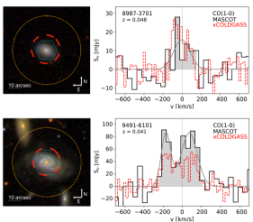
Figure 4: Comparison of xCOLDGASS and MASCOT observations for two targets the surveys have in common. We show the SDSS three color image, showing the MaNGA footprint (purple hexagon), the ARO beam (orange dashed circle) and the IRAM 30m beam of the xCOLDGASS observations (red dashed circle). The spectra on the right show the MASCOT CO(1-0) line spectrum (solid black line) and the xCOLDGASS spectrum (red dashed line). The area of the MASCOT spectrum between $v_{05}$ and $v_{95}$ is coloured in light grey.

3.8 ALMaQUEST Survey

The ALMaQUEST (ALMA-MaNGA QUEnching and STar formation) survey is a program with spatially-resolved 12CO(1-0) measurements obtained with the Atacama Large Millimeter Array (ALMA) for 46 galaxies from MaNGA DR15 (Lin et al., 2020). The aim of the ALMaQUEST survey is to investigate the dependence of star formation activity on the cold molecular gas content at kpc scales in nearby galaxies. While this survey spatially resolves the CO(1-0) line on scales matching the MaNGA resolution, its field-of-view is $\sim$ 50”, very similar to the MASCOT observations. The ALMaQUEST and MASCOT surveys have four sources in common (ID: 8952-6104, 8950-12705, 8450-6102 and 8655-3701) whose derived molecular gar masses agree well: $\log(M_{\rm{H_{2}},MASCOT}/M_{\odot}$) = 9.2 / 9.2 / 9.2 / 10.2, $\log(M_{\rm{H_{2},ALMaQUEST}}/M_{\odot}$) = 9.1 / 9.4 / 9.2 / 10.4). The ALMaQUEST Survey is thus well complementary to the MASCOT survey (see also Figure 2).

4 Results

4.1 Global Relations

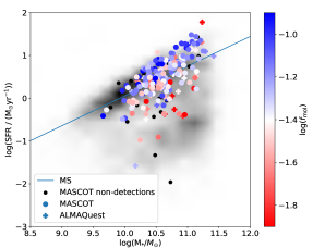
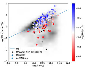
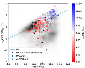
Figure 5: We show the distribution of sources in the SFR-M_∗ diagrams, colour-coded by the molecular gas mass fraction f$\rm{{}_{mol}=M_{H_{2}}/M_{*}}$ (upper left panel), the star formation efficiency $\rm{SFE=SFR/M_{H_{2}}}$ (upper right panel), and the molecular gas mass M${}_{H_{2}}$ (lower panel). For reference, we also show the distribution of the DR15 MaNGA sample in the SFR-M_∗ plane, as well as the star formation main sequence SFMS as derived by Whitaker et al. (2012). SFRs and stellar masses are both taken from the MaNGA-Pipe3D catalog for all sources, while the molecular gas masses are derived from the 55$\arcsec$ ARO beam for the MASCOT sources and from the MaNGA footprint for the ALMAQuest sources.

In Figure 5 we show the distribution of galaxies in the SFR–M_∗ plane. We complement the MASCOT sample with results from the ALMAQuest survey which mainly complements the MASCOT survey in the green valley. While we show the MASCOT non-detections in Figure 5 for completeness, the following analysis is limited to the 162 MASCOT-detected sources for which we can measure $\rm{M_{H_{2}}}$. Together with the 43 additional detected sources from the ALMAQuest survey, the following analysis focuses on a total sample size of 205 sources.

For consistency, and similar to Figure 2, for both the MASCOT and ALMAQuest samples, we use the SFR and M_∗ measurements provided by the Pipe3D catalog. We note that this differs to what is presented and shown in Table 3 and Figure 3 in the ALMAQuest paper by Lin et al. (2020) where the SFR is computed based on considering star-forming spaxels (as per BPT classification) within 1.5 R_eff.

We also remind the reader that the ALMAQuest molecular gas mass measurements were measured by summing the CO(1-0) flux over the areas within the MaNGA bundles while the MASCOT beam covers generally a larger area (beam size: 55 arcsec). This implies that the ALMAQuest molecular gas fractions may be lower when directly compared to the MASCOT molecular gas fractions. In the case of an underestimation of the CO(1-0) luminosity by 60% (as is the case for source 9491-6101 in comparison with the xCOLDGASS survey, see Section 3.7), $\log(\rm{f_{mol}})$ would be underestimated by 0.3.

The upper left panel of Figure 5 is color-coded by the molecular gas fraction defined as f$\rm{{}_{mol}=M_{H_{2}}/M_{*}}$. For the MASCOT sources, this fraction is directly computed using the $\rm{M_{H_{2}}}$ measurements described in Section 3.6 and M_∗ from the Pipe3D catalog. We measure a median molecular gas mass fraction for the MASCOT survey of f$\rm{{}_{mol}}=0.052$. For the ALMAQuest sources, we use the molecular gas masses reported in Table 3 in Lin et al. (2020) and the M_∗ from the Pipe3D catalog to compute f_mol.

The left panel of Figure 5 illustrates that f_mol is roughly constant along the SFMS and sharply drops below the SFMS. We observe a significant correlation with specific star formation rate ($\rm{sSFR=SFR/M_{*}}$) with a Spearman rank correlation coefficient of $r_{\rm{corr}}$=0.45 and a $p-$value of $1\times 10^{-11}$. The correlation with SFR alone is more moderate with $r_{\rm{corr}}=0.3$ and a $p-$value of $1\times 10^{-6}$, while we do not observe a significant correlation with stellar mass ($r_{\rm{corr}}$ = 0, $p-$value of $0.5$).

Similar trends are observed when we investigate how the molecular star formation efficiency $\rm{SFE=SFR/M_{H_{2}}}$ varies across the SFMS. The MASCOT median star formation efficiency is $\rm{\log(SFE/yr^{-1})=-8.7}$. The inverse of the SFE is the ‘depletion time’ $\tau_{\rm{dep}}$, indicating how much time is necessary to convert all the available molecular gas into stars at the current star formation rate. We find that the depletion time is roughly constant along the SFMS, as well, with depletion times dropping sharply below the SFMS. The correlation between both SFE and sSFR and SFE and SFR are significant with $r_{\rm{corr}}$= 0.68, $p-$value of $10^{-29}$ and $r_{\rm{corr}}=0.47$, $p-$value of $10^{-13}$, respectively. SFE seems to be independent of stellar mass, though ($r_{\rm{corr}}$ = 0, $p-$value of $0.2$).

In contrast to the first two panels of Figure 5, the lower panel shows that the molecular mass $\rm{M_{H_{2}}}$ varies strongly along the SFMS with significant correlations of $\rm{M_{H_{2}}}$ with both SFR and $\rm{M_{*}}$ ($\sim$ $r_{\rm{corr}}$ = 0.7 / 0.7, $p-$value = $10^{-31}$ / $p-$value = $10^{-36}$, respectively). The median molecular gas mass in the MASCOT sample is $\rm{\log(M_{H_{2}}/M_{\odot})}=9.3$.

The observed relations are similar and consistent with other studies in the literature. For example, Colombo et al. (2020) carried out a large CO(1-0) survey of 472 galaxies selected from the CALIFA survey with the APEX telescope and the CARMA array. The CALIFA-CO sample is of lower redshift than the MaNGA-CO observations presented here. Furthermore, their CO observations are measured from within $\sim 1\rm{R_{eff}}$ and therefore only measure the centrally available molecular gas. Despite these differences the observed relations between SFR, $\rm{M_{H_{2}}}$, f_mol, SFE and $\rm{M_{H_{2}}}$ are very similar to what we observe here. Similar conclusions were also made by Saintonge et al. (2017) with the xCOLDGASS survey. These observations imply that it is both the molecular gas mass fraction and the star formation efficiency that determines a galaxy’s position in the SFR–M_∗ plane.

We note that since we are using a prescription for $\alpha_{\rm{CO}}$ that is dependent on $\Delta\rm{(MS)}$, the derived quantities f_mol and SFE are dependent on M_∗ and SFR in a non-trivial way. We therefore re-peat the above analysis for a constant $\alpha_{\rm{CO}}$ and do not find significant changes in the trends reported in this Section. But even without the added dependency of $\alpha_{\rm{CO}}$ on $\Delta\rm{(MS)}$, derived quantities such as $\rm{SFE=SFR/M_{H_{2}}}$ and sSFR = $\rm{sSFR=SFR/M_{*}}$ are not independent and therefore some form of correlation is expected. Cicone et al. (2017) found that L_CO (from which M${}_{H_{2}}$ is derived) is strongly correlated with M_∗ and suggested that that this relation may be so tight and linear because the luminosity of optically thick low-$J$ CO transitions is an excellent tracer of the dynamical mass in star-forming galaxies, assuming that in this class of objects the bulk of CO probes molecular clouds in virial motions. We test this correlation with our observations and find a similarly tight correlation as Cicone et al. (2017) ($r_{\rm{corr}}$ = 0.84, $p-$value = $10^{-45}$, see Figure 6). We note the slight offset between the ALMAQuest data points and the MASCOT data points in Figure 6. As stated earlier, this is very likely due to the fact that the ALMAQuest molecular gas mass measurements were measured by summing the CO(1-0) flux over the areas within the MaNGA bundles while the MASCOT beam covers generally a larger area. Therefore, the total ALMAQuest CO measurements tend to be slightly underestimated, similar to our findings with the xCOLDGASS galaxies (see Section 3.7). Nevertheless, the best-fit regression parameters and correlation coefficients presented in Figure 6 are in very good agreement with the Cicone et al. (2017) results.

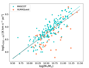
Figure 6: CO(1-0) line luminosity as a function of M_∗. The cyan solid line indicates the best fit linear relation obtained for the MASCOT data only ($y=-2.21+1.05x$), while the black dashed line indicates the best fit relation for the combined MASCOT and ALMAQuest samples ($y=-1.51+0.97x$).

4.2 Resolved Relations

While the above section reassuringly confirms previous results, the main aim and true strength of the MASCOT survey is to investigate how the molecular gas mass content relates to spatially resolved galaxy parameters. While an in-depth analysis of the resolved relations will be presented in upcoming papers in this series (Bertemes et al. in prep.), we present here an example of how the MASCOT survey is and will be used in investigating global CO measurements together with the spatially resolved nature of the MaNGA observations.

In Figure 7 we show how the molecular gas mass fraction, f_mol, relates to the stellar age gradient $\alpha_{\rm{age,LW}}$. The stellar age gradient describes the slope of the gradient of the luminosity-weighted log-age of the stellar population within a galactocentric distance of 0.5 to 2.0 R_eff). This measurement is provided as part of the Pipe3D catalog. While the Pipe3D catalog also reports mass-weighted ages, luminosity-weighted ages are more sensitive to small fractions of recent generations of stars (which contribute significantly in luminosity but not in mass), the mass-weighted age is more representative of the average epoch when the bulk of the stars in a galaxy formed (see e.g. Pasquali et al., 2010). Since we are investigating potential quenching, or recent star formation triggering effects, the luminosity weighted ages are more meaningful for this analysis. When $\alpha$ is positive, the stellar populations are getting older as we move away from the galactic center. When $\alpha$ is negative, it indicates that the stellar populations are getting younger as we move away from the galactic center. Despite the large scatter, we observe a weak positive correlation between $\alpha_{\rm{age,LW}}$ and f_mol ($r_{\rm{corr}}$ = 0.2, $p-$value=$4\times 10^{-3}$). The correlation is less weak when only considering galaxies with a negative $\alpha_{\rm{age,LW}}$ ($r_{\rm{corr}}$ = 0.3, $p-$value=$2\times 10^{-4}$). This means that galaxies with high molecular gas mass fractions tend to host younger stellar populations in their centres than they do at larger distances, while galaxies with low molecular gas mass fractions tend to be centrally quenched. This observation suggests that star formation quenching in these galaxies happens primarily inside-out and that a lower H₂ gas fraction seems to be a precursor of quenching.

Evidence for inside-out quenching being the dominant quenching mode has been suggested by other works (Lin et al., 2017; Bluck et al., 2020; Breda et al., 2020; Brownson et al., 2020). Such analyses have been in particular possible due to the emergence of large IFU galaxy surveys. For example, (Lin et al., 2019a) classify MaNGA galaxies into inside-out and outside-in quenching types. They base their classification on the strength and spatial distribution of quenched areas which are defined by two non-parametric parameters, quiescence and its concentration, traced by regions with low EW(H$\alpha$) (for details and the definitions of these parameters see Lin et al., 2019a). Additionally, they classify the galaxies based on their environment into satellites and centrals. They find that the fraction of inside-out quenching is systematically greater than that of outside-in quenching, suggesting that inside-out quenching is the dominant quenching mode in all environments.

AGN feedback or morphological quenching are potential mechanisms that may suppress the star formation and that may drive the features of the inside-out quenching but which one dominates under what circumstances is still an open point of debate (Lin et al., 2019a; Lin et al., 2017; Ellison et al., 2021c). The current size of the MASCOT sample and the parameter space it covers does not allow us yet to investigate this question in detail. But as the MASCOT sample continues to grow, we will address these topics in the forthcoming papers in this series.

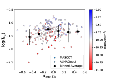
Figure 7: The molecular gas mass fraction f_mol as a function of stellar age gradient $\alpha_{\rm{age,LW}}$. Galaxies with lower f_mol tend to show older stellar populations close to the galactic center, while the opposite is true for galaxies with higher f_mol, potentially a signature for inside-out quenching being the dominant quenching mechanism in the MASCOT-MaNGA galaxies.

5 Conclusion

In this paper we have presented the first data release of the MASCOT survey which provides CO(1-0) measurements for galaxies that have already been observed as part of the SDSS-IV MaNGA survey. Observations are carried out with the 12m antenna at the Arizona Radio Observatory. We summarise the main points of this paper in the following:

1. This first data release presents CO(1-0) observations for 187 MaNGA galaxies. These galaxies are mostly located on and above the star formation main sequence and upcoming MASCOT observations are targeting primarily MaNGA galaxies on and below the star formation main sequence.

2. We develop a customised spectral line fitting technique to allow for a dynamic spectral binning of the spectra (from native binning up to spectral bins of 50 km/s) depending on the signal-to-noise ratio of the detection. To measure CO line fluxes, we allow secondary Gaussian components to account for broad, asymmetric line profiles and / or double-Gaussian features. We use non-parametric measurements to compute the flux and kinematics (velocity shift and velocity width) of the CO(1-0) emission line.

3. We use a metallicity- and sSFR-dependent $\alpha_{\rm{CO}}$ conversion factor to compute the total molecular gas mass within the beam size of the observations, 55 $\arcsec$.

4. The molecular gas mass fraction f$\rm{{}_{mol}=M_{H_{2}}/M_{*}}$ varies strongly across the star formation main sequence and correlates most strongly with sSFR (r${}_{corr}=0.45$) and SFR (r${}_{corr}=0.3$). Similar trends are observed for the star formation efficiency $\rm{SFE=SFR/M_{H_{2}}}$. SFE correlates strongly with sSFR (r${}_{corr}=0.68$) and SFR (r${}_{corr}=0.47$) but is mostly independent of stellar mass. These observations imply that it is both the molecular gas mass fraction and the star formation efficiency that determines a galaxy’s position the SFR-M_∗ plane, confirming previous results.

5. When investigating the MASCOT CO measurements in the context of the spatially resolved information from the supporting MaNGA data, we find that f_mol weakly correlates with the luminosity-weighted stellar age gradient $\alpha_{\rm{age,LW}}$. Galaxies with lower f_mol tend to show older stellar populations close to the galactic center, while the opposite is true for galaxies with higher f_mol, potentially a signature for inside-out quenching being the dominant quenching mechanism in the MASCOT-MaNGA galaxies.

The MASCOT survey is a large program and this data release only represents the first sets of observations of $\sim 800$ hours of observing time out of 1400 hours total. Upcoming data releases will present results for galaxies primarily on and below the star formation main sequence and the upcoming papers in this series (Bertemes et al. in prep., Wylezalek et al. in prep.) are investigating in depth the relations between molecular gas mass properties and spatially resolved diagnostics from the MaNGA observations. With the current survey efficiency, we expect the final MASCOT sample to consist of a total$\sim$ 250-300 galaxies.

Data Availability

The data underlying this article are available in the article and in its supplementary material. We also publish the data on the MASCOT website https://wwwstaff.ari.uni-heidelberg.de/dwylezalek/mascot.html.

Table 1: The MASCOT sample. In addition to the main galaxy parameters such as MaNGA ID, RA., Dec. and z, we list the SFR and stellar mass as reported in the MaNGA Pipe 3D Value Added Catalog. In column (7) we report the spectral binning $dv$ of the MASCOT spectra used in the analysis (see Section 3.5.1). In column (8), (9) and (10) we report the CO(1-0) line flux and luminosity measured as described in Section 3.5.2 and column (11) indicates if a one-Gaussian or two-Gaussian model was used to describe the line profile. In column (12) and (13) we report the non-parameteric velocity shift and velocity width of the CO(1-0) line (see Section 3.5.2). Column (14) and column (15) report the measured signal-to-noise ratios (see Section 3.5.2). Column (16) indicates whether the source was formally detected in the MASCOT survey (flag_CO=1) or whether the reported molecular gas mass (column 20) is an upper limit (flag_CO=2). In column (17) and column (18) we furthermore report the rms noise of the spectra in $dv$ in two different units and column (19) lists the metallicity and sSFR-dependent $\alpha_{\rm{CO}}$ conversion factor (see Section 3.6). The full table is available as supplementary material.

MaNGA ID	R.A.	Dec.	z	$\log(\rm{M_{*}})$	$\log(\rm{SFR})$	$dv$	SCO	LCO	LCO	NGauss	vmed	W90	W50	S/N	S/Npeak	flagCO	$\sigma_{\rm{rms,\lambda}}$	$\sigma_{\rm{rms,\nu}}$	$\alpha_{\rm{CO}}$	$\log(\rm{M_{H_{2}}})$
	deg.	deg.		$\log(\rm{M}_{\odot})$	$\log(\rm{M}_{\odot}/yr)$	km/s	erg s-1 cm-2	L⊙	K km s-1 pc2		km/s	km/s	km/s				erg s-1 cm-2 Å-1	mJy	M⊙(K km s-1 pc2)-1
10001-3702	132.91276	57.10742	0.026	10.11	-0.229	50	3.25e-17	1.28e+04	2.61e+08	1	1	218	90	4.9	4.0	1	6.52e-22	15.5	2.26	8.77
7443-12703	229.52557	42.74584	0.040	11.07	1.324	1	1.32e-16	1.32e+05	2.69e+09	2	48	317	100	32.1	6.6	1	2.40e-21	58.6	4.17	10.05
7443-12704	232.46105	42.62896	0.019	10.00	-0.468	50	6.49e-17	1.36e+04	2.77e+08	1	39	273	112	5.2	3.2	1	1.11e-21	25.8	3.62	9.00
7815-3702	317.90320	11.49694	0.029	10.47	0.263	50	4.79e-17	2.50e+04	5.11e+08	–	–	–	–	2.8	2.7	2	5.96e-22	14.2	1.99	9.01
7815-6104	319.19309	11.04374	0.081	11.18	0.985	50	6.11e-17	2.59e+05	5.29e+09	–	–	–	–	0.4	0.7	2	7.24e-22	19.2	8.56	10.66
7958-6101	257.38368	34.42703	0.024	10.44	0.223	50	5.34e-17	1.83e+04	3.73e+08	2	78	284	153	6.4	4.8	1	6.71e-22	15.8	1.91	8.85
7968-3701	322.21331	-1.07011	0.052	10.68	-0.017	50	8.90e-17	1.48e+05	3.02e+09	1	183	165	68	10.7	11.1	1	7.86e-22	19.5	1.65	9.70
7990-1902	264.52248	57.11816	0.030	10.74	0.738	50	4.95e-17	2.71e+04	5.53e+08	2	65	405	248	7.2	5.2	1	5.32e-22	12.7	2.12	9.07
7990-3703	262.09934	57.54541	0.029	10.40	0.805	50	1.58e-17	7.79e+03	1.59e+08	1	24	165	68	2.4	3.0	1	7.10e-22	16.9	8.62	9.14
7990-6104	261.60761	58.58885	0.026	10.29	0.644	50	8.36e-17	3.46e+04	7.05e+08	2	4	312	135	6.6	4.8	1	9.79e-22	23.2	4.12	9.46
7991-1901	258.54847	57.97609	0.093	10.43	1.280	50	2.44e-17	1.39e+05	2.83e+09	–	–	–	–	-0.5	0.7	2	2.86e-22	7.7	2.68	9.88
7992-6103	252.61893	64.02066	0.092	11.03	0.370	50	1.07e-17	6.05e+04	1.23e+09	1	63	412	169	3.4	2.2	1	2.45e-22	6.6	2.98	9.57
7992-6104	255.27948	64.67687	0.027	10.45	0.111	50	6.84e-17	3.04e+04	6.19e+08	1	39	228	93	9.4	6.5	1	6.73e-22	15.9	1.94	9.08
8077-12702	40.96904	0.15264	0.027	10.14	-0.044	50	1.59e-17	7.16e+03	1.46e+08	1	-33	473	194	2.8	2.1	1	5.00e-22	11.9	3.27	8.68
8077-12704	41.28056	0.95016	0.025	10.12	-0.354	50	1.42e-17	5.13e+03	1.05e+08	1	44	213	88	3.1	2.8	1	4.91e-22	11.6	2.98	8.49
8077-6102	40.55686	0.38294	0.022	9.96	-0.485	50	3.21e-17	9.34e+03	1.91e+08	1	-84	400	165	3.0	2.1	1	7.20e-22	16.9	2.91	8.74
8080-12702	47.99941	-1.16166	0.027	10.72	0.190	50	1.34e-16	5.79e+04	1.18e+09	1	35	590	242	8.1	4.0	1	1.13e-21	26.8	3.52	9.62
8082-12702	48.43841	-0.24146	0.026	11.10	0.230	50	1.23e-16	5.01e+04	1.02e+09	2	-32	447	233	6.7	4.4	1	1.30e-21	30.8	1.72	9.25
8082-9102	50.17993	-1.00229	0.036	10.74	0.611	50	1.23e-16	9.80e+04	2.00e+09	1	-11	454	187	7.5	4.3	1	1.13e-21	27.3	2.29	9.66
8084-12703	51.16991	-0.68147	0.039	10.87	0.651	50	4.82e-17	4.53e+04	9.24e+08	2	12	264	136	9.3	6.3	1	4.21e-22	10.3	2.48	9.36
8134-1901	113.40018	45.94337	0.077	10.98	1.174	50	5.59e-17	2.13e+05	4.34e+09	2	44	528	261	7.1	4.2	1	5.17e-22	13.5	2.81	10.09
8135-1902	114.09638	39.43827	0.118	11.16	1.433	50	2.55e-17	2.43e+05	4.96e+09	–	–	–	–	1.4	1.1	2	2.92e-22	8.2	2.68	10.12
8138-12703	116.38968	45.77232	0.032	10.96	-0.385	50	3.24e-17	1.98e+04	4.03e+08	1	7	624	256	4.8	2.5	1	4.42e-22	10.6	2.68	9.03
8146-1901	117.05386	28.22509	0.027	10.38	0.522	50	4.80e-17	2.12e+04	4.33e+08	–	–	–	–	2.2	1.4	2	5.99e-22	14.3	2.39	9.01
8150-9102	149.71387	32.07306	0.027	10.72	0.376	50	2.80e-17	1.24e+04	2.52e+08	1	-58	354	144	3.7	3.1	1	5.65e-22	13.4	2.41	8.78
8153-1901	41.00622	0.17629	0.023	9.99	-0.052	50	6.52e-17	2.00e+04	4.07e+08	1	-17	350	143	5.2	3.7	1	9.82e-22	23.1	2.12	8.94
8155-12701	53.17146	-1.18362	0.030	10.64	0.361	50	9.19e-17	5.17e+04	1.05e+09	2	-11	270	112	9.0	6.5	1	8.28e-22	19.8	2.64	9.44
8158-1901	60.85933	-5.49184	0.038	9.78	-0.213	50	1.74e-17	1.57e+04	3.20e+08	–	–	–	–	1.8	1.2	2	3.22e-22	7.8	6.21	9.30
8244-3701	132.38439	50.87412	0.027	10.48	-1.331	50	4.75e-17	2.14e+04	4.36e+08	–	–	–	–	0.3	1.2	2	5.92e-22	14.1	2.68	9.07
8249-3704	137.87476	45.46832	0.027	10.35	-0.068	50	4.22e-17	1.83e+04	3.74e+08	1	3	958	393	3.8	3.6	1	4.93e-22	11.7	3.62	9.13
8249-6102	137.33592	45.06551	0.051	10.53	0.909	50	3.25e-17	5.28e+04	1.08e+09	1	-5	165	68	4.4	5.9	1	6.68e-22	16.7	4.64	9.70
8250-6101	138.75314	42.02438	0.028	10.56	0.849	1	9.46e-17	4.44e+04	9.07e+08	2	-27	293	142	24.7	3.7	1	2.51e-21	59.9	2.95	9.43
8252-3701	144.84611	47.12686	0.027	10.63	-0.364	50	5.87e-17	2.63e+04	5.37e+08	1	4	764	315	4.7	3.5	1	6.97e-22	16.6	2.03	9.04
8252-9101	144.69238	48.56287	0.025	10.29	-0.221	50	4.15e-17	1.53e+04	3.13e+08	2	14	318	182	6.7	3.6	1	5.32e-22	12.6	2.50	8.89
8252-9102	145.54153	48.01286	0.056	10.81	1.195	50	2.94e-17	5.83e+04	1.19e+09	1	-17	197	82	5.5	4.5	1	4.83e-22	12.2	6.64	9.90
8253-12704	159.15328	43.50677	0.025	10.24	-0.975	50	3.11e-17	1.13e+04	2.31e+08	1	-28	305	126	5.0	3.7	1	5.05e-22	12.0	2.27	8.72
8255-12704	165.11773	44.26096	0.025	10.18	0.190	50	4.89e-17	1.87e+04	3.81e+08	1	51	452	186	6.7	4.8	1	5.28e-22	12.6	2.99	9.06
8257-12701	165.49581	45.22802	0.020	10.63	0.813	2	1.91e-16	4.56e+04	9.31e+08	1	27	164	67	29.7	5.8	1	4.45e-21	104.3	3.07	9.46
8257-9102	166.76743	45.82213	0.025	10.64	0.041	50	7.41e-17	2.83e+04	5.78e+08	2	-27	476	270	6.3	3.7	1	8.23e-22	19.5	2.24	9.11
8259-3704	179.59330	43.81527	0.070	10.88	0.831	50	2.09e-17	6.58e+04	1.34e+09	1	-140	520	213	3.0	2.6	1	4.57e-22	11.8	1.94	9.42
8262-3702	183.65983	43.53621	0.024	10.39	0.302	50	1.39e-17	4.90e+03	9.99e+07	1	-69	165	68	2.9	2.9	1	4.73e-22	11.2	5.45	8.74
8262-9102	184.55356	44.17324	0.025	10.66	0.894	1	1.04e-16	3.76e+04	7.67e+08	1	47	282	116	29.5	4.6	1	2.44e-21	57.8	2.38	9.26
8311-3703	205.01217	23.14297	0.032	10.84	0.561	50	1.33e-16	8.09e+04	1.65e+09	2	-20	324	193	13.0	8.0	1	8.76e-22	21.0	1.99	9.52
8313-12702	240.67741	41.19726	0.033	10.73	0.861	50	1.25e-16	8.50e+04	1.73e+09	2	2	282	150	9.2	5.8	1	1.17e-21	28.1	4.13	9.85
8313-6102	240.91243	41.15305	0.034	10.73	-1.962	50	9.99e-17	7.10e+04	1.45e+09	–	–	–	–	0.5	0.9	2	1.24e-21	29.4	2.68	9.59
8317-6102	194.92502	43.75317	0.058	11.13	1.120	50	5.86e-17	1.23e+05	2.52e+09	2	-16	475	294	8.1	4.3	1	5.17e-22	13.1	2.05	9.71
8318-12702	196.44403	46.46185	0.025	10.62	-0.164	50	1.52e-16	5.65e+04	1.15e+09	2	-56	361	210	8.7	5.6	1	1.37e-21	32.4	3.34	9.59
8318-9101	196.08628	45.05665	0.028	10.30	0.582	50	2.89e-17	1.40e+04	2.85e+08	–	–	–	–	1.9	1.5	2	5.40e-22	12.8	6.90	9.29
8319-9101	202.53348	48.89326	0.071	11.06	1.144	50	3.19e-17	1.02e+05	2.09e+09	1	9	178	74	6.8	7.4	1	4.13e-22	10.7	2.14	9.65
8320-9101	206.31385	23.31651	0.030	10.48	0.684	50	6.36e-17	3.40e+04	6.93e+08	1	29	242	99	5.4	4.4	1	1.06e-21	25.3	6.34	9.64
8322-1901	198.78424	30.40377	0.023	10.38	0.458	50	1.01e-16	3.25e+04	6.63e+08	1	150	657	270	5.9	4.0	1	9.67e-22	22.8	2.26	9.18
8322-3701	199.06648	30.26453	0.049	11.01	1.142	50	6.44e-17	9.71e+04	1.98e+09	2	9	527	270	4.2	2.7	1	9.45e-22	23.2	4.37	9.94
8326-6102	215.01790	47.12133	0.070	11.03	0.744	50	3.72e-17	1.18e+05	2.41e+09	–	–	–	–	2.2	2.7	2	4.45e-22	11.5	3.65	9.95

MaNGA ID	R.A.	Dec.	z	$\log(\rm{M})$	$\log(\rm{SFR})$	$dv$	SCO	LCO	LCO	NGauss	vmed	W90	W50	S/N	S/Npeak	flagCO	$\sigma_{\rm{rms,\lambda}}$	$\sigma_{\rm{rms,\nu}}$	$\alpha_{\rm{CO}}$	$\log(\rm{M_{H_{2}}})$
	deg.	deg.		$\log(\rm{M}_{\odot})$	$\log(\rm{M}_{\odot}/yr)$	km/s	erg s-1 cm-2	L⊙	K km s-1 pc2		km/s	km/s	km/s				erg s-1 cm-2 Å-1	mJy	M⊙(K km s-1 pc2)-1
8329-12701	213.41682	43.86656	0.035	10.84	0.832	50	1.26e-16	9.42e+04	1.92e+09	1	27	511	210	8.7	5.0	1	9.08e-22	21.9	2.05	9.59
8330-12703	203.37460	40.52967	0.027	10.42	0.394	50	2.64e-17	1.15e+04	2.36e+08	1	13	234	96	4.3	3.1	1	5.72e-22	13.7	2.31	8.74
8331-3703	204.15019	43.37336	0.053	10.55	0.622	50	3.47e-17	6.00e+04	1.22e+09	1	-100	235	97	3.0	2.7	1	1.07e-21	26.6	2.44	9.47
8331-6102	205.91886	41.69582	0.075	11.18	0.925	50	5.08e-17	1.85e+05	3.78e+09	2	35	254	127	6.5	5.0	1	6.07e-22	15.8	2.21	9.92
8332-3702	207.87280	43.80642	0.033	10.56	0.650	50	2.75e-17	1.86e+04	3.79e+08	1	27	332	136	4.3	2.8	1	5.45e-22	13.1	3.64	9.14
8332-9102	210.24094	42.85564	0.032	10.60	0.060	50	1.17e-16	7.43e+04	1.52e+09	1	17	460	188	12.3	7.1	1	6.68e-22	16.1	2.66	9.61
8335-12705	216.75986	39.95721	0.025	10.52	0.562	50	8.51e-17	3.28e+04	6.69e+08	1	20	296	121	6.5	4.8	1	1.06e-21	25.1	2.80	9.27
8338-12701	172.05119	21.99684	0.021	9.96	0.178	50	2.03e-17	5.39e+03	1.10e+08	1	3	166	68	3.8	4.4	1	5.36e-22	12.7	10.07	9.04
8341-12704	189.21325	45.65117	0.030	10.72	0.724	1	5.03e-17	2.81e+04	5.72e+08	1	69	164	67	22.2	5.0	1	1.91e-21	45.7	2.68	9.19
8439-12704	144.03108	50.43922	0.064	10.86	0.799	50	5.27e-17	1.37e+05	2.80e+09	1	33	503	206	7.4	4.1	1	4.50e-22	11.5	2.79	9.89
8440-6104	135.75896	40.43398	0.029	10.67	-0.056	50	5.46e-17	2.73e+04	5.57e+08	–	–	–	–	2.3	2.5	2	6.80e-22	16.2	2.68	9.17
8442-12701	197.66878	32.22818	0.049	10.53	0.804	50	4.07e-17	6.06e+04	1.24e+09	1	62	277	113	5.1	3.9	1	6.83e-22	16.9	4.62	9.76
8442-6101	200.27335	31.83129	0.061	10.79	0.777	50	3.39e-17	8.09e+04	1.65e+09	1	20	390	160	4.5	3.3	1	5.57e-22	14.1	2.09	9.54
8446-1901	205.75333	36.16565	0.024	10.04	-0.549	50	1.28e-16	4.28e+04	8.74e+08	–	–	–	–	0.5	0.5	2	2.39e-21	55.7	4.91	9.63
8450-6102	171.74883	21.14167	0.042	10.43	0.818	50	1.87e-17	2.01e+04	4.10e+08	1	-3	165	68	3.0	4.6	1	5.53e-22	13.5	3.88	9.20
8452-12705	157.93769	46.67167	0.025	10.33	0.394	50	5.55e-17	2.08e+04	4.24e+08	2	-93	277	144	5.1	4.4	1	8.79e-22	20.8	4.25	9.26
8452-1902	157.77930	48.01483	0.059	10.76	0.869	50	1.16e-17	2.53e+04	5.16e+08	1	63	181	75	2.8	2.8	1	4.01e-22	10.1	6.15	9.50
8453-3704	154.48083	46.60328	0.030	10.18	-0.093	50	1.56e-17	8.51e+03	1.74e+08	1	39	193	80	3.6	3.5	1	4.43e-22	10.7	3.03	8.72
8454-12702	153.04902	45.14215	0.076	11.13	1.444	50	3.47e-17	1.31e+05	2.68e+09	1	194	609	249	4.4	2.7	1	4.68e-22	12.2	4.07	10.04
8455-3701	157.17945	39.83888	0.029	10.34	0.340	50	4.16e-17	2.16e+04	4.41e+08	1	-12	361	148	5.1	4.3	1	6.02e-22	14.4	2.92	9.11
8459-1901	147.80179	44.00930	0.016	9.71	-0.271	50	2.81e-17	4.11e+03	8.39e+07	1	24	259	106	4.2	3.0	1	5.76e-22	13.4	2.68	8.35
8462-9101	144.52643	36.0392	0.022	10.07	-0.074	50	2.55e-17	7.74e+03	1.58e+08	1	58	229	95	3.8	2.9	1	6.94e-22	16.4	2.18	8.54
8464-3704	188.10783	44.18361	0.031	10.60	0.708	50	6.51e-17	3.74e+04	7.64e+08	1	17	165	68	7.2	8.0	1	7.75e-22	18.6	1.85	9.15
8465-9102	198.18916	46.93498	0.028	10.40	0.100	50	6.29e-17	2.91e+04	5.93e+08	1	54	536	219	5.8	3.6	1	6.83e-22	16.2	2.60	9.19
8466-12702	167.96743	45.54139	0.028	10.40	0.516	50	4.51e-17	2.21e+04	4.50e+08	2	16	312	169	5.6	5.0	1	6.36e-22	15.2	3.62	9.21
8483-6101	246.45691	48.10033	0.020	10.44	0.251	50	1.01e-16	2.37e+04	4.84e+08	1	29	362	149	5.2	3.9	1	1.49e-21	34.9	2.00	8.99
8547-6102	217.32486	52.66555	0.030	10.54	0.293	50	4.24e-17	2.39e+04	4.87e+08	1	33	361	148	4.5	2.9	1	7.02e-22	16.8	2.07	9.00
8548-12704	244.07472	47.98160	0.021	10.27	0.082	50	6.34e-17	1.61e+04	3.29e+08	1	-18	267	110	5.7	3.9	1	1.03e-21	24.2	4.02	9.12
8550-12703	247.67443	40.52938	0.030	10.49	0.492	50	6.67e-17	3.59e+04	7.33e+08	1	42	165	67	6.5	7.8	1	8.95e-22	21.3	2.15	9.20
8551-12705	233.94092	44.83479	0.030	10.59	0.920	50	6.86e-17	3.65e+04	7.45e+08	2	9	387	92	6.0	6.6	1	8.16e-22	19.4	4.06	9.48
8552-12701	226.43166	44.40490	0.028	10.66	0.163	50	5.44e-17	2.64e+04	5.39e+08	2	-101	484	334	6.2	4.0	1	6.64e-22	15.8	3.89	9.32
8553-1901	233.96834	57.90263	0.030	10.77	0.671	50	4.48e-17	2.48e+04	5.06e+08	–	–	–	–	2.4	1.8	2	5.57e-22	13.3	2.68	9.13
8553-9102	234.54184	57.60365	0.074	11.24	1.097	50	4.69e-17	1.64e+05	3.35e+09	2	19	427	205	5.4	3.5	1	5.75e-22	14.9	2.18	9.86
8588-12705	250.31287	39.75235	0.030	10.63	0.727	50	6.57e-17	3.62e+04	7.38e+08	1	-2	417	172	5.4	2.8	1	9.12e-22	21.9	2.76	9.31
8588-6101	248.45675	39.26320	0.032	10.88	0.599	50	8.69e-17	5.33e+04	1.09e+09	1	36	195	80	9.5	8.5	1	8.77e-22	21.0	2.21	9.38
8592-6101	222.67177	51.70446	0.026	10.54	0.376	50	7.13e-17	2.90e+04	5.92e+08	2	34	337	188	9.1	5.6	1	6.39e-22	15.2	3.16	9.27
8595-3703	221.43798	51.58081	0.030	10.91	0.362	50	1.43e-16	7.59e+04	1.55e+09	1	104	566	232	7.5	3.8	1	1.27e-21	30.4	2.61	9.61
8595-6104	219.39661	51.58313	0.044	10.87	-0.364	50	2.70e-17	3.18e+04	6.49e+08	1	4	165	68	5.0	5.3	1	5.10e-22	12.6	2.68	9.24
8600-1901	242.58522	43.00964	0.025	10.19	0.493	50	1.52e-17	5.81e+03	1.18e+08	1	-10	166	68	2.8	3.0	1	5.86e-22	13.9	4.84	8.76
8600-3704	245.84527	41.65118	0.027	10.49	0.640	50	9.36e-17	4.22e+04	8.61e+08	2	7	284	151	9.5	5.6	1	8.61e-22	20.5	2.68	9.36
8601-12702	247.59167	40.92424	0.031	9.65	-0.413	50	3.23e-17	1.83e+04	3.73e+08	1	26	174	71	5.8	4.7	1	5.87e-22	14.0	2.68	9.00
8603-12704	247.89387	40.56559	0.027	10.78	0.702	50	1.46e-16	6.59e+04	1.34e+09	2	-9	355	204	15.6	11.9	1	7.47e-22	17.8	2.68	9.56
8603-6103	247.80036	40.42187	0.027	10.14	0.113	50	4.36e-17	1.92e+04	3.92e+08	1	64	314	128	5.5	3.9	1	6.26e-22	14.9	2.68	9.02
8603-6104	247.41995	40.68695	0.031	10.55	-0.004	50	3.02e-17	1.71e+04	3.48e+08	–	–	–	–	2.7	2.7	2	3.75e-22	9.0	3.52	9.09
8604-12702	246.65449	39.12754	0.035	10.72	0.744	50	5.04e-17	3.84e+04	7.84e+08	1	41	382	157	6.0	4.1	1	6.21e-22	15.0	3.32	9.42
8604-9102	246.45535	40.34520	0.029	10.49	0.882	50	3.82e-17	1.95e+04	3.97e+08	1	-13	382	157	6.2	4.2	1	4.71e-22	11.2	7.86	9.49
8615-3701	321.00791	-0.36632	0.062	10.86	0.808	50	2.84e-17	6.88e+04	1.40e+09	1	108	248	101	3.8	3.7	1	6.28e-22	15.9	4.09	9.76
8618-3704	318.86228	9.75781	0.070	10.94	0.889	50	3.65e-17	1.16e+05	2.36e+09	1	-16	203	83	6.7	6.7	1	5.08e-22	13.1	2.17	9.71
8624-12702	260.58171	59.07653	0.030	10.57	0.598	50	7.22e-17	3.95e+04	8.06e+08	1	9	412	168	5.2	3.3	1	1.03e-21	24.6	3.16	9.41
8624-12703	264.23953	59.20028	0.031	10.56	0.405	50	6.97e-17	3.98e+04	8.13e+08	1	-2	383	157	3.1	1.9	1	1.69e-21	40.0	2.67	9.34
8626-12701	263.52527	56.79961	0.029	10.46	-0.433	50	3.98e-17	2.06e+04	4.21e+08	–	–	–	–	2.1	1.6	2	4.96e-22	11.8	4.73	9.30
8626-12702	263.20536	56.90127	0.029	10.64	0.485	50	6.81e-17	3.56e+04	7.25e+08	2	19	335	164	7.9	5.1	1	6.79e-22	16.3	3.19	9.36
8626-12704	263.75521	57.05243	0.047	10.70	0.811	50	2.95e-17	4.09e+04	8.34e+08	–	–	–	–	0.2	1.1	2	5.41e-22	13.3	35.63	10.47
8626-3702	261.72122	56.84880	0.028	10.56	0.525	50	1.03e-16	4.82e+04	9.83e+08	2	-19	456	258	10.4	4.5	1	7.22e-22	17.2	2.16	9.33
8626-3703	264.66254	56.82424	0.029	10.33	0.297	50	4.11e-17	2.15e+04	4.39e+08	2	11	254	126	5.5	4.8	1	5.57e-22	13.3	2.60	9.06
8655-3701	356.75182	-0.44738	0.071	11.16	1.282	50	8.30e-17	2.70e+05	5.51e+09	1	7	335	137	6.5	4.4	1	1.01e-21	26.3	2.51	10.14

MaNGA ID	R.A.	Dec.	z	$\log(\rm{M})$	$\log(\rm{SFR})$	$dv$	SCO	LCO	LCO	NGauss	vmed	W90	W50	S/N	S/Npeak	flagCO	$\sigma_{\rm{rms,\lambda}}$	$\sigma_{\rm{rms,\nu}}$	$\alpha_{\rm{CO}}$	$\log(\rm{M_{H_{2}}})$
	deg.	deg.		$\log(\rm{M}_{\odot})$	$\log(\rm{M}_{\odot}/yr)$	km/s	erg s-1 cm-2	L⊙	K km s-1 pc2		km/s	km/s	km/s				erg s-1 cm-2 Å-1	mJy	M⊙(K km s-1 pc2)-1
8712-6101	118.72692	53.84627	0.035	10.91	1.273	1	1.43e-16	1.06e+05	2.17e+09	1	16	249	103	38.2	5.8	1	2.65e-21	64.0	2.26	9.69
8713-6104	118.31731	39.05012	0.041	10.93	0.936	50	7.49e-17	7.70e+04	1.57e+09	2	26	275	142	7.5	5.7	1	8.01e-22	19.6	2.41	9.58
8713-9102	118.85539	39.18609	0.033	10.52	0.414	50	3.25e-17	2.17e+04	4.44e+08	2	108	509	237	5.6	4.2	1	3.62e-22	8.7	2.68	9.08
8715-3702	119.92067	50.83997	0.054	10.79	0.965	50	1.33e-17	2.47e+04	5.04e+08	1	-3	184	76	3.2	2.5	1	4.35e-22	10.9	2.68	9.13
8717-3704	117.51833	34.47931	0.029	10.60	0.456	1	1.48e-16	7.52e+04	1.53e+09	2	-37	319	184	38.9	6.0	1	2.46e-21	58.8	2.01	9.49
8727-12705	57.10409	-6.62606	0.021	10.42	0.672	50	1.51e-16	3.97e+04	8.09e+08	1	9	165	67	12.1	19.0	1	1.10e-21	25.9	3.28	9.42
8727-3701	54.90496	-5.63293	0.021	10.19	-0.161	50	1.68e-17	4.39e+03	8.96e+07	–	–	–	–	1.8	1.6	2	3.16e-22	7.4	3.11	8.44
8932-9102	196.65170	27.87294	0.021	10.16	0.138	50	6.23e-17	1.63e+04	3.33e+08	1	-1	428	176	3.2	2.2	1	1.46e-21	34.2	3.44	9.06
8935-6104	195.53290	27.64831	0.023	10.28	0.314	50	5.73e-17	1.82e+04	3.71e+08	1	-43	217	89	5.6	5.0	1	9.24e-22	21.7	2.34	8.94
8940-1902	120.98712	25.48072	0.073	11.10	1.276	50	5.85e-17	2.00e+05	4.07e+09	1	10	403	166	7.5	4.1	1	5.46e-22	14.2	2.31	9.97
8944-6103	147.65106	34.77714	0.053	10.75	0.775	50	4.30e-17	7.44e+04	1.52e+09	2	-3	338	210	5.5	4.5	1	5.78e-22	14.5	2.05	9.49
8945-12701	171.89808	47.37939	0.033	10.30	0.708	50	1.27e-17	8.28e+03	1.69e+08	1	13	165	67	2.3	3.4	1	5.48e-22	13.1	7.24	9.09
8946-6101	168.75209	46.63452	0.054	10.73	0.824	50	3.60e-17	6.63e+04	1.35e+09	2	26	316	154	8.0	5.6	1	3.55e-22	8.9	2.08	9.45
8947-12701	171.02709	48.69629	0.058	11.14	0.217	50	5.24e-17	1.10e+05	2.24e+09	2	-73	611	364	6.4	3.6	1	5.34e-22	13.5	2.98	9.82
8947-1901	171.38369	51.18040	0.027	10.38	0.556	50	6.38e-17	2.83e+04	5.78e+08	1	28	227	93	6.4	4.8	1	9.30e-22	22.1	2.84	9.22
8947-9101	168.73450	50.33487	0.047	10.90	0.963	50	4.46e-17	6.15e+04	1.26e+09	1	18	187	76	5.3	5.2	1	8.15e-22	20.1	2.68	9.53
8950-12705	194.73313	27.83344	0.025	10.53	-0.060	50	9.74e-17	3.69e+04	7.53e+08	1	51	534	219	6.3	3.4	1	1.03e-21	24.5	2.06	9.19
8952-6104	204.93397	27.77647	0.028	10.33	0.459	50	5.05e-17	2.43e+04	4.96e+08	1	11	165	67	6.6	10.1	1	6.38e-22	15.2	3.22	9.20
8978-3701	248.50746	41.34794	0.028	10.34	0.150	50	3.73e-17	1.82e+04	3.71e+08	1	29	248	101	5.0	3.9	1	7.14e-22	17.0	2.68	9.00
8979-3704	244.42296	40.93381	0.062	10.68	0.283	50	1.69e-17	4.13e+04	8.42e+08	1	40	269	110	3.4	3.2	1	5.56e-22	14.1	3.11	9.42
8979-6102	241.82338	41.40360	0.035	10.53	0.396	50	2.73e-17	2.00e+04	4.07e+08	2	19	303	169	3.8	3.0	1	5.42e-22	13.1	2.44	9.00
8982-9101	201.71365	26.59123	0.023	10.24	0.340	50	1.81e-17	5.98e+03	1.22e+08	1	-84	335	137	2.8	2.0	1	5.68e-22	13.4	4.49	8.74
8987-3701	136.24988	28.34772	0.049	10.37	0.674	50	1.11e-17	1.63e+04	3.33e+08	1	-4	281	115	2.9	3.0	1	3.71e-22	9.2	3.40	9.05
8989-9102	177.52435	50.46744	0.024	10.27	0.111	50	4.49e-17	1.49e+04	3.05e+08	1	16	267	110	7.2	4.6	1	5.72e-22	13.5	1.89	8.76
8993-12705	165.39153	45.65386	0.029	10.46	0.374	50	1.03e-16	5.38e+04	1.10e+09	1	-13	527	217	8.5	6.0	1	7.84e-22	18.7	4.54	9.70
8993-6104	166.53203	45.12225	0.021	8.04	-1.187	50	3.25e-17	8.75e+03	1.79e+08	–	–	–	–	1.9	2.7	2	6.12e-22	14.4	5.61	9.00
8996-3703	172.30201	53.73396	0.027	10.44	0.345	50	6.36e-17	2.85e+04	5.81e+08	2	17	296	146	8.5	5.5	1	6.50e-22	15.5	2.09	9.08
8997-12704	170.16277	52.62504	0.048	11.12	0.478	50	3.89e-17	5.66e+04	1.16e+09	2	185	704	514	4.1	2.8	1	5.86e-22	14.5	2.40	9.44
9000-1901	171.40065	54.38257	0.021	10.34	-0.075	50	1.91e-17	4.89e+03	9.98e+07	1	-11	242	99	2.9	2.5	1	5.78e-22	13.5	2.68	8.43
9024-1902	224.43778	33.16563	0.030	9.90	0.356	50	3.07e-17	1.68e+04	3.43e+08	–	–	–	–	2.3	2.3	2	5.73e-22	13.7	2.68	8.96
9027-12701	243.93592	31.96395	0.032	10.77	1.045	50	1.35e-16	8.13e+04	1.66e+09	2	5	650	211	9.6	8.0	1	8.68e-22	20.8	2.68	9.65
9029-12702	247.25172	41.28426	0.032	10.80	0.731	50	1.69e-16	1.05e+05	2.13e+09	1	22	164	67	13.8	14.6	1	1.16e-21	27.8	1.90	9.61
9029-6102	246.39291	41.68139	0.028	10.03	0.298	50	3.28e-17	1.54e+04	3.15e+08	2	-28	403	263	3.0	3.5	1	7.42e-22	17.7	3.76	9.07
9034-1901	226.72354	47.05696	0.088	11.07	0.970	50	4.67e-17	2.38e+05	4.85e+09	2	12	265	114	9.3	7.0	1	4.08e-22	10.9	2.42	10.07
9034-3702	226.28032	46.96365	0.038	10.18	0.500	50	1.73e-17	1.51e+04	3.08e+08	–	–	–	–	2.3	2.4	2	3.21e-22	7.8	6.17	9.28
9036-9102	240.56931	42.91689	0.024	10.21	0.327	50	1.19e-16	4.26e+04	8.70e+08	2	36	233	108	10.2	8.0	1	1.09e-21	25.8	2.68	9.37
9038-3702	237.51955	42.30863	0.021	10.05	0.250	50	2.93e-17	7.44e+03	1.52e+08	1	9	164	67	3.4	5.4	1	7.21e-22	16.9	3.33	8.70
9041-12701	236.94151	28.64169	0.033	10.49	0.465	2	1.48e-16	9.94e+04	2.03e+09	1	24	193	80	25.2	5.5	1	3.80e-21	91.4	2.25	9.66
9042-12703	235.15267	28.51243	0.033	10.71	-0.013	50	6.67e-17	4.35e+04	8.88e+08	1	11	443	181	5.2	3.4	1	9.24e-22	22.3	2.11	9.27
9042-6101	232.55107	27.13411	0.033	10.54	-0.909	50	2.06e-17	1.33e+04	2.72e+08	1	173	382	156	3.8	1.9	1	4.49e-22	10.8	2.68	8.86
9044-6101	230.68698	29.76960	0.023	10.24	0.275	50	6.46e-17	2.03e+04	4.15e+08	2	49	386	188	6.3	4.4	1	7.58e-22	17.9	2.46	9.01
9047-6104	248.14087	26.38073	0.059	11.25	1.104	50	1.21e-16	2.63e+05	5.37e+09	2	-41	586	294	8.6	3.9	1	9.12e-22	23.1	2.43	10.12
9049-6104	248.46298	25.86004	0.051	10.80	0.837	50	2.62e-17	4.29e+04	8.76e+08	2	43	513	282	3.9	2.7	1	4.37e-22	10.9	1.99	9.24
9050-3704	245.99500	22.39336	0.037	10.74	1.054	50	1.04e-16	8.70e+04	1.77e+09	1	2	233	96	8.0	6.6	1	1.17e-21	28.3	2.68	9.68
9050-9101	245.99843	21.79503	0.032	10.61	0.577	50	5.13e-17	3.22e+04	6.57e+08	1	-1	242	99	6.7	5.9	1	7.02e-22	16.9	2.00	9.12
9085-12703	260.30627	29.18589	0.047	10.61	0.021	50	7.67e-17	1.06e+05	2.17e+09	–	–	–	–	2.6	2.2	2	9.38e-22	23.1	1.74	9.58
9095-1901	242.81005	24.22502	0.033	10.62	0.396	50	7.78e-17	5.01e+04	1.02e+09	1	66	275	113	7.5	5.1	1	9.11e-22	21.9	1.72	9.24
9095-9102	243.08488	23.00202	0.032	10.65	0.725	50	6.04e-17	3.82e+04	7.80e+08	2	43	295	148	6.0	3.9	1	8.30e-22	19.9	1.82	9.15
9185-9101	256.21228	34.81733	0.056	11.21	1.354	50	9.97e-17	1.99e+05	4.07e+09	1	46	285	116	11.4	7.6	1	7.03e-22	17.7	3.20	10.11
9195-3702	27.84278	13.06033	0.064	11.14	0.628	50	4.09e-17	1.07e+05	2.19e+09	2	-29	583	337	5.8	3.3	1	4.24e-22	10.9	2.68	9.77
9196-6103	260.35471	54.30492	0.030	10.55	0.255	50	4.12e-17	2.23e+04	4.54e+08	2	60	384	216	4.5	3.8	1	6.79e-22	16.2	2.05	8.97
9196-6104	262.31771	54.20592	0.079	10.93	0.991	50	3.60e-17	1.46e+05	2.98e+09	1	58	300	122	3.4	2.7	1	8.68e-22	22.7	2.04	9.78
9485-12705	121.77993	36.23347	0.032	10.86	0.548	50	7.44e-17	4.72e+04	9.64e+08	1	-13	701	287	9.4	5.2	1	4.45e-22	10.7	3.22	9.49
9485-1901	120.77803	37.02355	0.071	10.96	1.272	50	6.62e-17	2.16e+05	4.40e+09	1	6	165	68	9.9	12.7	1	5.49e-22	14.2	2.24	10.00
9485-3701	119.53203	36.83126	0.039	10.13	-0.162	50	1.53e-17	1.45e+04	2.95e+08	1	-52	353	144	3.4	2.3	1	3.58e-22	8.7	2.01	8.77
9486-12701	121.67826	39.09021	0.042	10.96	0.593	50	7.19e-17	7.64e+04	1.56e+09	2	34	446	262	7.3	5.7	1	6.86e-22	16.8	2.68	9.62
9486-12702	121.12959	40.20604	0.040	10.84	0.571	50	6.68e-17	6.66e+04	1.36e+09	2	1	274	142	13.3	10.0	1	4.08e-22	9.9	2.56	9.54
9487-3702	123.33054	46.14715	0.054	10.58	-0.321	50	3.17e-17	5.76e+04	1.18e+09	–	–	–	–	2.0	2.5	2	3.85e-22	9.7	2.68	9.50
9487-3703	124.81375	45.29875	0.043	10.33	0.673	50	2.02e-17	2.34e+04	4.78e+08	1	7	387	159	4.3	2.9	1	3.43e-22	8.4	3.93	9.27
9487-9102	123.82032	46.07525	0.041	11.00	0.951	50	1.02e-16	1.05e+05	2.15e+09	1	112	317	130	12.0	8.5	1	6.79e-22	16.6	3.18	9.83
9491-1902	120.04224	19.23433	0.078	11.08	0.720	50	3.10e-17	1.23e+05	2.51e+09	2	-3	625	360	6.4	3.6	1	2.93e-22	7.7	2.68	9.83

MaNGA ID	R.A.	Dec.	z	$\log(\rm{M})$	$\log(\rm{SFR})$	$dv$	SCO	LCO	LCO	NGauss	vmed	W90	W50	S/N	S/Npeak	flagCO	$\sigma_{\rm{rms,\lambda}}$	$\sigma_{\rm{rms,\nu}}$	$\alpha_{\rm{CO}}$	$\log(\rm{M_{H_{2}}})$
	deg.	deg.		$\log(\rm{M}_{\odot})$	$\log(\rm{M}_{\odot}/yr)$	km/s	erg s-1 cm-2	L⊙	K km s-1 pc2		km/s	km/s	km/s				erg s-1 cm-2 Å-1	mJy	M⊙(K km s-1 pc2)-1
9491-6101	119.174377409	17.99116	0.041	10.90	1.284	50	9.55e-17	1.00e+05	2.04e+09	2	3	417	244	9.1	5.0	1	7.37e-22	18.0	4.18	9.93
9494-3704	128.019903751	21.62862	0.054	10.75	0.940	50	4.02e-17	7.29e+04	1.49e+09	1	7	397	163	7.4	4.1	1	3.91e-22	9.8	2.42	9.56
9497-12705	118.074345115	19.59508	0.117	10.905	1.728	50	3.66e-17	3.42e+05	6.99e+09	–	–	–	–	-1.2	0.3	2	4.19e-22	11.8	2.68	10.27
9500-1901	131.725410562	25.37008	0.051	10.86	0.638	50	3.69e-17	5.95e+04	1.21e+09	–	–	–	–	0.6	1.3	2	4.50e-22	11.2	2.68	9.51
9506-3701	133.569904521	27.26652	0.064	11.06	1.484	50	8.59e-17	2.22e+05	4.54e+09	1	4	188	77	14.5	13.3	1	5.31e-22	13.6	2.06	9.97
9508-12705	127.273132937	25.77262	0.028	10.54	0.235	50	4.19e-17	1.96e+04	4.00e+08	1	31	552	226	4.8	3.5	1	5.63e-22	13.4	2.27	8.96
9508-6101	127.13101957	26.34868	0.053	10.59	0.800	50	4.63e-17	8.15e+04	1.66e+09	1	9	486	201	3.9	2.8	1	6.77e-22	17.0	4.37	9.86
9508-6104	127.553016498	26.62732	0.053	10.80	0.772	50	4.10e-17	7.21e+04	1.47e+09	1	37	301	123	4.7	3.5	1	7.11e-22	17.8	1.93	9.45
9509-3702	122.439749732	25.88030	0.025	10.10	0.401	50	3.56e-17	1.35e+04	2.75e+08	–	–	–	–	2.7	2.2	2	6.67e-22	15.8	10.06	9.44
9865-9102	224.897977138	49.32744	0.027	10.37	0.708	50	2.59e-17	1.12e+04	2.28e+08	1	-33	187	76	4.5	3.7	1	6.24e-22	14.8	5.54	9.10
9870-3702	229.934607505	44.32184	0.028	10.58	0.325	50	4.09e-17	1.97e+04	4.01e+08	1	31	216	89	4.0	3.3	1	9.94e-22	23.7	2.94	9.07
9871-6101	227.863793703	41.08999	0.031	10.39	0.627	50	4.11e-17	2.36e+04	4.81e+08	2	36	275	145	5.1	4.5	1	6.33e-22	15.2	3.53	9.23
9872-3701	233.231957146	42.43825	0.020	10.13	-0.102	50	2.48e-17	5.73e+03	1.17e+08	1	-18	235	97	3.3	2.8	1	6.64e-22	15.5	3.40	8.60
9881-12705	205.373570269	23.16696	0.031	10.69	0.273	50	7.70e-17	4.40e+04	8.98e+08	2	96	273	143	6.3	5.1	1	1.03e-21	24.7	2.08	9.27
9881-3702	203.81165409	25.04475	0.026	10.40	0.485	50	6.10e-17	2.50e+04	5.11e+08	2	4	262	134	9.5	6.2	1	5.55e-22	13.2	1.77	8.96
9888-12704	236.006339163	28.27702	0.033	10.73	0.720	50	7.40e-17	4.97e+04	1.01e+09	2	55	275	143	9.7	6.0	1	6.45e-22	15.5	2.96	9.48
9888-12705	236.901377571	26.06376	0.032	10.94	0.777	50	1.20e-16	7.24e+04	1.48e+09	1	-4	466	191	9.1	6.1	1	9.18e-22	22.1	2.60	9.59

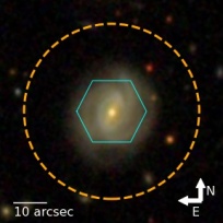
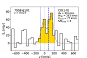
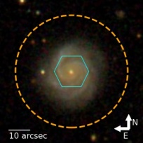
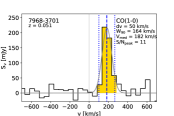
Figure 9: continued.

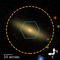
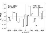
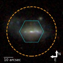
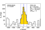
Figure 10: continued.

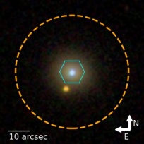
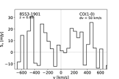
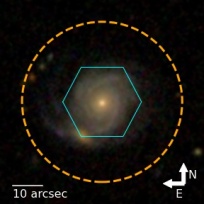
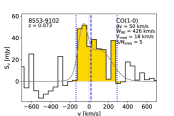
Figure 11: continued.

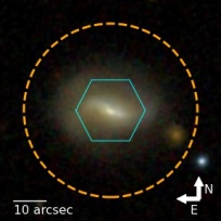
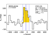
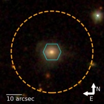
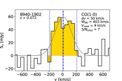
Figure 12: continued.

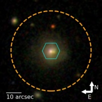
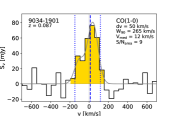
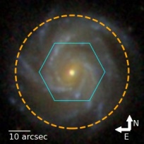
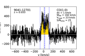
Figure 13: continued.

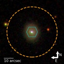
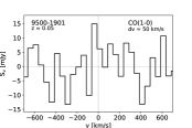
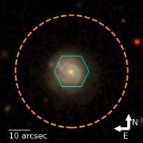
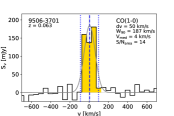
Figure 14: continued.

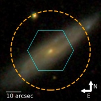
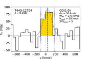
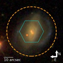
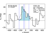
Figure 15: continued.

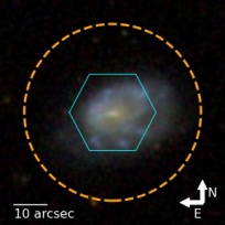
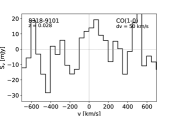
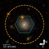
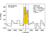
Figure 16: continued.

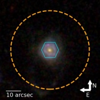
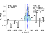
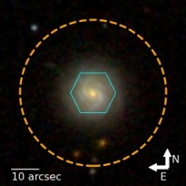
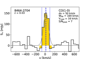
Figure 17: continued.

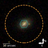
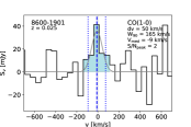
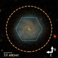
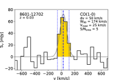
Figure 18: continued.

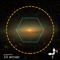
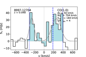
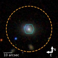
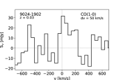
Figure 19: continued.

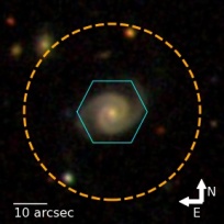
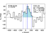
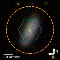
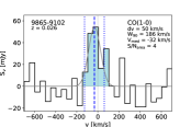
Figure 20: continued.

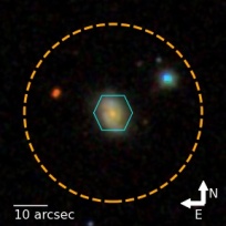
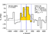
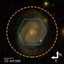
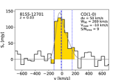
Figure 21: continued.

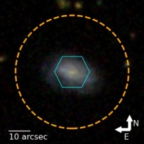
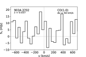
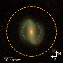
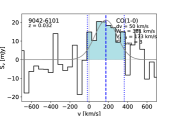
Figure 22: continued.

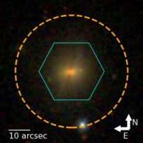
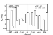
Figure 23: continued.

References

- Abolfathi et al. (2018) Abolfathi B., et al., 2018, The Astrophysical Journal Supplement Series, 235, 42
- Accurso et al. (2017) Accurso G., et al., 2017, MNRAS, 470, 4750
- Aguado et al. (2019a) Aguado D. S., et al., 2019a, ApJS, 240, 23
- Aguado et al. (2019b) Aguado D. S., et al., 2019b, ApJS, 240, 23
- Barrera-Ballesteros et al. (2020) Barrera-Ballesteros J. K., et al., 2020, MNRAS, 492, 2651
- Barrera-Ballesteros et al. (2021) Barrera-Ballesteros J. K., et al., 2021, MNRAS,
- Belfiore et al. (2019) Belfiore F., et al., 2019, AJ, 158, 160
- Blanton et al. (2011) Blanton M. R., Kazin E., Muna D., Weaver B. A., Price-Whelan A., 2011, AJ, 142, 31
- Blanton et al. (2017) Blanton M. R., et al., 2017, AJ, 154, 28
- Bluck et al. (2020) Bluck A. F. L., et al., 2020, MNRAS, 499, 230
- Bolatto et al. (2013) Bolatto A. D., Wolfire M., Leroy A. K., 2013, ARA&A, 51, 207
- Bolatto et al. (2017) Bolatto A. D., et al., 2017, ApJ, 846, 159
- Bothwell et al. (2014) Bothwell M. S., et al., 2014, MNRAS, 445, 2599
- Bouché et al. (2010) Bouché N., et al., 2010, ApJ, 718, 1001
- Breda et al. (2020) Breda I., et al., 2020, A&A, 635, A177
- Brownson et al. (2020) Brownson S., Belfiore F., Maiolino R., Lin L., Carniani S., 2020, MNRAS, 498, L66
- Bundy et al. (2015) Bundy K., et al., 2015, ApJ, 798, 7
- Cappellari (2017) Cappellari M., 2017, MNRAS, 466, 798
- Cappellari & Emsellem (2004) Cappellari M., Emsellem E., 2004, PASP, 116, 138
- Cappellari et al. (2011) Cappellari M., et al., 2011, MNRAS, 413, 813
- Cherinka et al. (2018) Cherinka B., Sánchez-Gallego J., Andrews B., Brownstein J., 2018, sdss/marvin: Marvin Beta, doi:10.5281/zenodo.596700, https://doi.org/10.5281/zenodo.596700
- Cherinka et al. (2019) Cherinka B., et al., 2019, AJ, 158, 74
- Cicone et al. (2017) Cicone C., et al., 2017, A&A, 604, A53
- Colombo et al. (2018) Colombo D., et al., 2018, MNRAS, 475, 1791
- Colombo et al. (2020) Colombo D., et al., 2020, arXiv e-prints, p. arXiv:2009.08383
- Combes et al. (2007) Combes F., Young L. M., Bureau M., 2007, MNRAS, 377, 1795
- Croom et al. (2012) Croom S. M., et al., 2012, MNRAS, 421, 872
- Dey et al. (2019) Dey B., et al., 2019, MNRAS, 488, 1926
- Drory et al. (2015) Drory N., et al., 2015, AJ, 149, 77
- Ellison et al. (2020a) Ellison S. L., Thorp M. D., Pan H.-A., Lin L., Scudder J. M., Bluck A. F. L., Sánchez S. F., Sargent M., 2020a, MNRAS, 492, 6027
- Ellison et al. (2020b) Ellison S. L., et al., 2020b, MNRAS, 493, L39
- Ellison et al. (2021a) Ellison S. L., Lin L., Thorp M. D., Pan H.-A., Scudder J. M., Sánchez S. F., Bluck A. F. L., Maiolino R., 2021a, MNRAS, 501, 4777
- Ellison et al. (2021b) Ellison S. L., Lin L., Thorp M. D., Pan H.-A., Sánchez S. F., Bluck A. F. L., Belfiore F., 2021b, MNRAS, 502, L6
- Ellison et al. (2021c) Ellison S. L., et al., 2021c, MNRAS, 505, L46
- Gunn et al. (2006) Gunn J. E., et al., 2006, AJ, 131, 2332
- Güsten et al. (2006) Güsten R., Nyman L. Å., Schilke P., Menten K., Cesarsky C., Booth R., 2006, A&A, 454, L13
- Harrison (2017) Harrison C. M., 2017, Nature Astronomy, 1, 0165
- Kennicutt (1998a) Kennicutt Jr. R. C., 1998a, ARA&A, 36, 189
- Kennicutt (1998b) Kennicutt Jr. R. C., 1998b, ApJ, 498, 541
- Law et al. (2015) Law D. R., et al., 2015, AJ, 150, 19
- Law et al. (2016) Law D. R., et al., 2016, AJ, 152, 83
- Law et al. (2021) Law D. R., et al., 2021, AJ, 161, 52
- Leung et al. (2018) Leung G. Y. C., et al., 2018, MNRAS, 477, 254
- Levy et al. (2018) Levy R. C., et al., 2018, ApJ, 860, 92
- Levy et al. (2019) Levy R. C., et al., 2019, ApJ, 882, 84
- Lilly et al. (2013) Lilly S. J., Carollo C. M., Pipino A., Renzini A., Peng Y., 2013, ApJ, 772, 119
- Lin et al. (2017) Lin L., et al., 2017, ApJ, 851, 18
- Lin et al. (2019a) Lin L., et al., 2019a, ApJ, 872, 50
- Lin et al. (2019b) Lin L., et al., 2019b, ApJ, 884, L33
- Lin et al. (2020) Lin L., et al., 2020, arXiv e-prints, p. arXiv:2010.01751
- Liu et al. (2013) Liu G., Zakamska N. L., Greene J. E., Nesvadba N. P. H., Liu X., 2013, MNRAS, 436, 2576
- Maiolino et al. (2008) Maiolino R., et al., 2008, A&A, 488, 463
- Masters et al. (2019) Masters K. L., et al., 2019, MNRAS, 488, 3396
- Pasquali et al. (2010) Pasquali A., Gallazzi A., Fontanot F., van den Bosch F. C., De Lucia G., Mo H. J., Yang X., 2010, MNRAS, 407, 937
- Péroux & Howk (2020) Péroux C., Howk J. C., 2020, ARA&A, 58, 363
- Pettini & Pagel (2004) Pettini M., Pagel B. E. J., 2004, MNRAS, 348, L59
- Rupke (2018) Rupke D., 2018, Galaxies, 6, 138
- Saintonge et al. (2011) Saintonge A., et al., 2011, MNRAS, 415, 32
- Saintonge et al. (2016) Saintonge A., et al., 2016, MNRAS, 462, 1749
- Saintonge et al. (2017) Saintonge A., et al., 2017, ApJS, 233, 22
- Salpeter (1955) Salpeter E. E., 1955, ApJ, 121, 161
- Sánchez et al. (2012) Sánchez S. F., et al., 2012, A&A, 538, A8
- Sánchez et al. (2016) Sánchez S. F., et al., 2016, Rev. Mex. Astron. Astrofis., 52, 21
- Sanchez et al. (2017a) Sanchez S. F., et al., 2017a, preprint, (arXiv:1709.05438)
- Sánchez et al. (2017b) Sánchez S. F., et al., 2017b, MNRAS, 469, 2121
- Sanders & Mirabel (1985) Sanders D. B., Mirabel I. F., 1985, ApJ, 298, L31
- Smee et al. (2013) Smee S. A., et al., 2013, AJ, 146, 32
- Solomon et al. (1997) Solomon P. M., Downes D., Radford S. J. E., Barrett J. W., 1997, ApJ, 478, 144
- Tumlinson et al. (2017) Tumlinson J., Peeples M. S., Werk J. K., 2017, ARA&A, 55, 389
- Utomo et al. (2017) Utomo D., et al., 2017, ApJ, 849, 26
- Wake et al. (2017) Wake D. A., et al., 2017, AJ, 154, 86
- Westfall et al. (2019) Westfall K. B., et al., 2019, AJ, 158, 231
- Whitaker et al. (2012) Whitaker K. E., van Dokkum P. G., Brammer G., Franx M., 2012, ApJ, 754, L29
- Wylezalek et al. (2018) Wylezalek D., Zakamska N. L., Greene J. E., Riffel R. A., Drory N., Andrews B. H., Merloni A., Thomas D., 2018, MNRAS, 474, 1499
- Wylezalek et al. (2020) Wylezalek D., Flores A. M., Zakamska N. L., Greene J. E., Riffel R. A., 2020, MNRAS, 492, 4680
- Yan et al. (2016a) Yan R., et al., 2016a, AJ, 151, 8
- Yan et al. (2016b) Yan R., et al., 2016b, AJ, 152, 197
- Young et al. (2011) Young L. M., et al., 2011, MNRAS, 414, 940