Interpretability Aware Model Training to Improve Robustness against Out-of-Distribution Magnetic Resonance Images in Alzheimer’s Disease Classification

Abstract

Owing to its pristine soft-tissue contrast and high resolution, structural magnetic resonance imaging (MRI) is widely applied in neurology, making it a valuable data source for image-based machine learning (ML) and deep learning applications. The physical nature of MRI acquisition and reconstruction, however, causes variations in image intensity, resolution, and signal-to-noise ratio. Since ML models are sensitive to such variations, performance on out-of-distribution data, which is inherent to the setting of a deployed healthcare ML application, typically drops below acceptable levels. We propose an interpretability aware adversarial training regime to improve robustness against out-of-distribution samples originating from different MRI hardware. The approach is applied to 1.5T and 3T MRIs obtained from the Alzheimer’s Disease Neuroimaging Initiative database. We present preliminary results showing promising performance on out-of-distribution samples.

1 Introduction

Magnetic resonance (MR) imaging produces high resolution, high contrast, three dimensional (3D) anatomical representations based on local variations in magnetic susceptibility (Duyn et al., 2007). Scan quality, quantified by the signal-to-noise ratio and image resolution, varies depending on the imaging sequence, hardware (e.g. magnetic field strength, choice of coils, and shimming correction), and reconstruction software (Rutt and Lee, 1996; Ladd et al., 2018) in addition to tissue characteristics (Bloem et al., 2018). In clinical practice, 1.5T scanners provide a reasonable compromise between scan quality and imaging/machine cost. Improved signal-to-noise ratios are achieved with 3T scanners, which are therefore preferable if a high level of morphological detail is required, e.g. in neurological studies of the brain. Differences between scans originating from different hard-/software are generally subtle and usually would not impact diagnosis by a human observer. However, deep learning models are very vulnerable to small shifts in the data distribution and non-robust models do not generalize to such out-of-distribution (OOD) samples. Models trained on images acquired using the same protocol and scanner generalize poorly to data acquired using different imaging protocols or hardware (Allen et al., 2019; Bluemke et al., 2020; Lee et al., 2020). Models perform particularly poorly on scans of lower quality than that used for training (Guan et al., 2021). In practice, real world data is acquired using a variety of scanners and protocols in different clinics. The training data will therefore never be representative of all examples a model may encounter upon deployment. So far, only models trained with multiple curated data sets or strongly augmented data have been able to achieve some amount of generalization (Chen et al., 2020; Mårtensson et al., 2020; Zhang et al., 2020). A similar challenge is provided by $L_{\infty}$ adversarial attacks, which disturb input data minimally to produce substantial changes in the output of the classifier. Since individual pixel values only change subtly, the perturbations are often invisible to the human observer, but will fool a classifier nevertheless. Recently, Boopathy et al. (2020) have shown that adversarial examples which successfully fool a classifier often fail to prevent 2-class interpretation discrepancies from occurring. Penalizing a network based on 2-class interpretation discrepancies during training improves adversarial robustness. We hypothesize that robustness to adversarial attacks could also increase OOD robustness, hence improving the generalization ability of medical image classifiers. This idea motivated our study, which investigates interpretability aware adversarial training as a means to improve OOD robustness in the realm of MR imaging. This preliminary analysis applies the presented concept to Alzheimer’s disease classification. We train convolutional neural networks (CNNs) on high quality MR images acquired at a specific magnetic field strength (3T) and test on lower quality OOD images (1.5T).

2 Methods

2.1 Model

Following Brüningk et al. (2021), we use simple 2D and 3D CNNs comprising three convolutional layers with batch normalization, ReLU activation and max pooling, followed by a fully connected layer. Dropout is applied to the flattened outputs of the last convolutional layer. L2 regularization was used on the weights of all layers. Hyperparameter optimization is described in A.2.

2.2 Interpretability Measure

Grad-CAM is a widely-used posthoc interpretability method to visualize the evidence on which a classifier bases its decisions (Selvaraju et al., 2017). In contrast to other approaches such as CAM (Zhou et al., 2016), it does not constrain the model architecture. Given a class-specific prediction $y^{c}$, Grad-CAM calculates weights $n_{m}^{c}$, $m\in\{1,\dots,n\}$, to weigh the (3D) convolutional output maps $f_{1},\dots,f_{n}$,

$$n_{m}^{c}=\frac{1}{|xyz|}\sum_{x}\sum_{y}\sum_{z}\frac{\partial y^{c}}{\partial f_{xyz}^{m}}.$$ (1)

The output maps are multiplied by the corresponding weights to arrive at the class activation map,

$$I^{c}=ReLu\left(\sum_{m}n_{m}^{c}f^{m}\right).$$ (2)

2.3 Training Regimes

We compared three baseline training regimes (normal, combined, and adversarial) to the proposed interpretability aware adversarial approach. The normal and combined baselines minimize the standard binary cross-entropy loss function $L$,

$$L=\frac{-1}{n}\sum_{i}^{n}y_{i}\cdot\log\hat{y}_{i}+(1-y_{i})\cdot\log(1-\hat{y}_{i})$$ (3)

where $y_{1}\dots y_{n}$ are the labels associated with the benign examples $x_{1}\dots x_{n}$ and $\hat{y}_{i}\dots\hat{y}_{n}$ are the corresponding predictions.
Models trained under the adversarial regime initially use the standard cross-entropy loss function (3). After 400 steps, we include adversarial examples generated using the projected gradient descent (PGD) algorithm (Madry et al., 2018) and apply an adversarial cross-entropy loss function $L_{adv}$,

$$\begin{split}L_{adv}=&\frac{-1}{n}\sum_{i}^{n}y_{i}\cdot\log\hat{y}_{adv,i}+\\ &(1-y_{i})\cdot\log(1-\hat{y}_{adv,i}),\end{split}$$ (4)

where $\hat{y}_{adv,1}\dots\hat{y}_{adv,n}$ are the adversarial predictions. Very briefly, the PGD attack adds disturbances that depend on an iterative gradient calculation. The disturbances are clipped to the $[-\epsilon,\epsilon]$ domain to control the strength of the attack. For training, we first linearly increase $\epsilon$ over 2000 steps. Training then continues at maximum attack strength until early stopping (scoring validation loss) is triggered. We used a custom learning rate scheduler, too (20% learning rate reduction upon plateau). We evaluated perturbation sizes $\epsilon\in\{0.001,0.005\}$.
We define a measure of the $\ell_{1}$ 2-class interpretation discrepancy

$$\begin{split}\tilde{D}_{2,\ell_{1}}\left(x,x_{adv}\right)=&\frac{1}{2}\left(\|I(x,c_{1})-I(x_{adv},c_{1})\|_{1}+\right.\\ &\left.\|I(x,c_{2})-I(x_{adv},c_{2})\|_{1}\right),\end{split}$$ (5)

where $I(x,c)$ denotes a class-specific (either class $c_{1}$ or $c_{2}$) activation map generated by Grad-CAM following eq:map. Training of the interpretability aware model follows the process outlined above for adversarial training but now the model switches to an adjusted loss $L_{adj}$ combining the adversarial cross-entropy loss with the measure of the $\ell_{1}$ 2-class interpretation discrepancy,

$$L_{adj}=L_{adv}+\lambda\tilde{D}_{2,\ell_{1}}\left(x,x_{adv,\epsilon}\right),$$ (6)

where the regularization parameter $\lambda>0$ controls the balance between performance on adversarial examples and class activation map similarity. We investigated values of $\lambda$ ranging from 1 to 30.

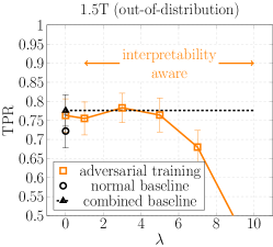
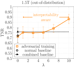
fig:metrics_1_out [TPR]  [TNR]   [ACC]

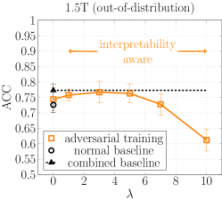
Figure 0: 2D OOD performance metrics shown as a function of $\lambda$ (no further improvement for $\lambda>5$). Performance is evaluated on undisturbed OOD (1.5T) data. The adversarial model ($\lambda=0$) and the interpretability aware models ($\lambda>0$) were trained using $\boldsymbol{\epsilon=0.001}$.

3 First Experiments

3.1 Data

We test our approach on structural, T1-weighted MR images of Alzheimer’s disease (AD) and cognitive normal (CN) subjects from the Alzheimer’s Disease Neuroimaging Initiative (ADNI) database. 1.5T (n=358, mean prevalence of AD=0.55) and 3T (n=247, mean prevalence of AD=0.35) images of non-overlapping subjects were included. Data pre-processing and image subset selection is described in A.1.

3.2 Performance Evaluation

The normal baseline, the adversarial model, and the interpretability aware models were trained on 3T data (within-distribution, WD) whereas the combined baseline trained on both 1.5T and 3T data. All models were evaluated on (i) undisturbed 3T data, (ii) adversarial examples generated from 3T data, and (iii) 1.5T data (OOD). We performed 5-fold nested cross validation and report results calculated on the held out test sets in Fig. 1. All results were averaged over all folds and three repeated runs to report means $\pm$ standard deviations. We evaluated test set prediction accuracy, TPR (sensitivity), TNR (specificity), and areas under the receiver operator (AUC) and precision recall curves (APS, i.e. AUPRC).

4 Results

We first evaluate normal and combined baseline performance on OOD vs WD data in tab:normal. As expected, performance degrades if training and testing magnetic field strengths differ, but improves if both 1.5T and 3T scans are seen during training. fig:TPR_1_out,fig:TNR_1_out,fig:ACC_1_out compare the OOD performance of the 2D adversarial ($\lambda=0$, $\epsilon_{train}=0.001$) and interpretability aware models ($\lambda>0$, $\epsilon_{train}=0.001$) to that of the baselines. AUROC and AUPRC scores as well as WD metrics are provided in the appendix. In line with results reported by Boopathy et al. (2020), the interpretability aware model is more robust to adversarial examples compared to the model trained with adversarial attacks but without interpretation discrepancy penalties (fig:TPR_1_in–fig:APS_1_in). Increased adversarial robustness translated into a small improvement in OOD performance: 0.78 (interpretability aware, $\lambda=3$) vs 0.76 (adversarial), 0.75 vs 0.71, and 0.77 vs 0.74 TPR, TNR, and ACC. The OOD performance of the best interpretability aware models approaches that of the combined baseline trained on both 1.5T and 3T images. Compared to the normal baseline, the best interpretability aware models ($\lambda\in\{3,5\}$) perform significantly better (p<0.05, Mann-Whitney U test). These trends were observed both in the $\epsilon_{train}=0.001$ and $\epsilon_{train}=0.005$ (fig:TPR_5_out–fig:APS_5_out) setting. Preliminary results in the 3D setting (fig:3D_TPR_1_out–fig:3D_APS_1_out) show that the 3D interpretability aware model is superior to the adversarial model and the normal baseline on the 1.5T data, too. Representative examples of Grad-CAM saliency maps of OOD examples obtained with and without interpretability aware training are shown in the appendix (fig:tn_c0_int–S7). In the latter case, we observe that clinically meaningful explanations highlighting tissue atrophy as AD evidence are obtained.

5 Discussion

In the healthcare domain, model generalization to OOD data is an immanent challenge given the variety in hardware and post-processing algorithms. Additionally, model interpretability is essential to build trust in clinical ML predictions (Ahmad et al., 2018; Carvalho et al., 2019) – it is a natural next step to harness this concept for an alternative, intuitive method to increase model robustness. Following previous work (Boopathy et al., 2020), we extended the proposed approach to be compliant with 2D/3D MR data, implemented Grad-CAM as interpretability measure, and, as a novel use case, demonstrate that this approach improves OOD robustness. Following careful hyperparameter optimization, we show that increased adversarial robustness translates into improved OOD robustness against images obtained using varying hardware. Interpretability aware training could hence be a complementary concept to (extreme) data augmentation and training on heterogeneous inputs, which were previously suggested to improve model generalizability (Chen et al., 2020; Mårtensson et al., 2020; Zhang et al., 2020). Given its intuitive conceptualization, interpretability aware training may be well-accepted by the clinical community, too. Notably, the used data set was greatly harmonized, which may limit the potential benefit of interpretability aware adversarial training. Specifically, ADNI MR images were acquired using a unified protocol (Jack et al., 2008) including scanner-specific pre-scan procedures and a phantom calibration scan prior to every patient imaging. The procedure was designed to harmonize scans and hence strongly exceeds the normal standards of clinical practice. Thus, the evaluation on the ADNI data should only be considered a preliminary analysis and we plan to test our approach in a more realistic setting using images from the UK Biobank, OASIS and the Health-RI Parelsnoer Neurodegenerative Diseases Biobank as true external validation sets. Moreover, we are planning to further investigate the use of different interpretability methods. Grad-CAM relies on up-sampling the final class activation map and hence suffers from poor resolution. Recently, LayerCAM has been proposed as an effective means to mitigate this limitation by weighting each image pixel using the backward class-specific gradients, yielding more fine-grained visualizations (Jiang et al., 2021). However, saliency map reproducibility and localization ability has previously been criticized in the context of complex models trained on medical image classification tasks (Arun et al., 2021). Here, we use a simple model driven by the clinical hallmarks of AD (Brüningk et al., 2021). Also, the model does not interpret the meaningfulness of the Grad-CAM representations but uses a quantitative measure of salience map differences as a regularizing term only. Finally, a strong assumption of this study was that adversarial examples can be used to mimic the variation of MR images induced by physical processes. We provide preliminary data based on PGD attacks, but it is also important to test on unseen attacks and compare attacks in general. Examples could include Gabor, Snow (Kang et al., 2019), and $\ell_{1}$ attacks (Chen et al., 2018).
We have presented here a preliminary analysis of interpretability aware training to boost OOD performance on medical MR images which poses an important challenge in the field of ML for healthcare.

This work was partially funded and supported by the Swiss National Science Foundation (Spark grants 190466 (B.R.) and 190647 (S.C.B., C.R.J); Ambizione Grant #PZ00P3186101, C.R.J). Since October 2021 the work of SCB was supported by the Botnar Research Centre for Child Health Postdoctoral Excellence Programme under PEP-2021-1008. Data collection and sharing for this project was funded by the Alzheimer’s Disease Neuroimaging Initiative (ADNI) (National Institutes of Health Grant U01 AG024904) and DOD ADNI (Department of Defense award number W81XWH-12-2-0012). ADNI is funded by the National Institute on Aging, the National Institute of Biomedical Imaging and Bioengineering, and through generous contributions from the following: AbbVie, Alzheimer’s Association; Alzheimer’s Drug Discovery Foundation; Araclon Biotech; BioClinica, Inc.; Biogen; Bristol-Myers Squibb Company; CereSpir, Inc.; Cogstate; Eisai Inc.; Elan Pharmaceuticals, Inc.; Eli Lilly and Company; EuroImmun; F. Hoffmann-La Roche Ltd and its affiliated company Genentech, Inc.; Fujirebio; GE Healthcare; IXICO Ltd.; Janssen Alzheimer Immunotherapy Research & Development, LLC.; Johnson & Johnson Pharmaceutical Research & Development LLC.; Lumosity; Lundbeck; Merck & Co., Inc.; Meso Scale Diagnostics, LLC.; NeuroRx Research; Neurotrack Technologies; Novartis Pharmaceuticals Corporation; Pfizer Inc.; Piramal Imaging; Servier; Takeda Pharmaceutical Company; and Transition Therapeutics. The Canadian Institutes of Health Research is providing funds to support ADNI clinical sites in Canada. Private sector contributions are facilitated by the Foundation for the National Institutes of Health (www.fnih.org). The grantee organization is the Northern California Institute for Research and Education, and the study is coordinated by the Alzheimer’s Therapeutic Research Institute at the University of Southern California. ADNI data are disseminated by the Laboratory for Neuro Imaging at the University of Southern California.

Appendix A Supplementary Methods

A.1 Data preparation

All images were preprocessed using the fmriprep pipeline for bias-field correction, reference space registration, and skull stripping, as previously described in Brüningk et al. (2021). Images were intensity normalized (mean zero and unit variance) and segmented into functional brain subunits using the CerebrA atlas (Manera et al., 2020). It was recently demonstrated that constraining the model input to clinically relevant brain subunits boosted performance (Brüningk et al., 2021). Hence, we train our models on the image subset comprising only the left hippocampus (3D models, $33\times 46\times 48$ voxels) or a selected 2D slice ($30\times 36$ voxels) comprising part of the left hippocampus and amygdala – both of these structures are highly affected by neurodegeneration in the early stages of AD (Jack et al., 2005; Knafo, 2012).

A.2 Hyperparameters

Model hyperparameters were optimized as previously described in Brüningk et al. (2021). The 2D model consists of three convolutional layers ($4\times 4\times 4$) and one fully connected layer. Convolutional layer inputs are padded such that the outputs have the same height and width as the inputs. Every convolutional layer is followed by a batch normalization layer, an activation layer (ReLU), and a max pooling layer ($2\times 2$). The first two convolutional layers have 8 filters and the last convolutional layer has 16 filters. Dropout ($p=0.5$) is applied to the flattened outputs of the last convolutional layer. L2 regularization ($\lambda=0.001$) was applied to the weights of all layers. HPs associated with adversarial/interpretability aware training were optimized with grid search to maximize adversarial robustness.

The architecture of the 3D model was equivalent to that the 2D model. 2D convolutional and pooling layers were replaced with the corresponding 3D implementations. The learning rate, batch size, kernel sizes, and hyperparameters related to L2 regularization, dropout, and adversarial/interpretability aware training were kept constant. However, it is likely that the parameters relating to the adversarial attack and the interpretation discrepancy measure need further optimization.

Models were trained for a maximum of 3000 epochs on NVIDIA TITAN RTX, 24 GiB RAM GPUs using the Adam optimizer and a learning rate of 0.0003. Weights were initialized using the He method (He et al., 2015). The models return the raw (pre-softmax) score of the sample for each of the two classes in the model.

Appendix B Supplementary Results

tab:normal

Table S1: Comparing normal and combined baseline performance on benign 1.5T and 3T examples. * Not evaluated.

Test	3T					1.5T
Train	ACC	TPR	TNR	AUC	APS	ACC	TPR	TNR	AUC	APS
2D-1.5T	0.82	0.78	0.80	0.90	0.86	0.75	0.79	0.70	0.85	0.87
2D-3T	0.88	0.79	0.90	0.94	0.90	0.73	0.72	0.72	0.82	0.85
2D-3T/1.5T	0.87	0.83	0.88	0.93	0.90	0.77	0.78	0.76	0.85	0.87
3D-1.5T	*	*	*	*	*	0.87	0.90	0.83	0.93	0.93
3D-3T	0.88	0.75	0.94	0.95	0.92	0.44	0.20	0.73	0.50	0.60
3D-3T/1.5T	0.88	0.77	0.92	0.94	0.90	0.82	0.84	0.81	0.91	0.92

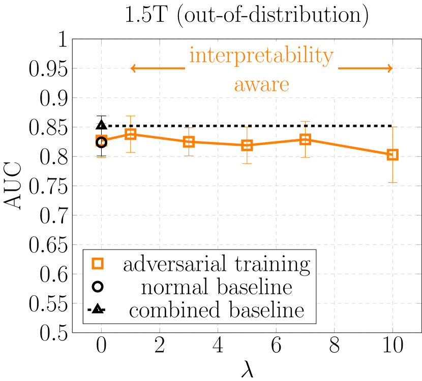
fig:suppl_1_out [AUC]  [APS]

Figure S0: 2D OOD performance metrics shown as a function of $\lambda$. Performance is evaluated on 2D OOD (1.5T) data. The adversarial model ($\lambda=0$) and the interpretability aware models ($\lambda>0$) were trained using $\boldsymbol{\epsilon=0.001}$. The ‘normal’ and ‘combined’ baseline indicated by a circle and a triangle are trained on undisturbed data.

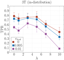
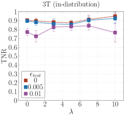
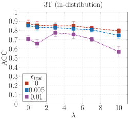
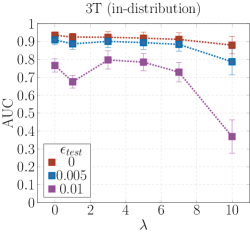
fig:suppl_1_in [TPR]  [TNR]   [ACC]   [AUC]  [APS]

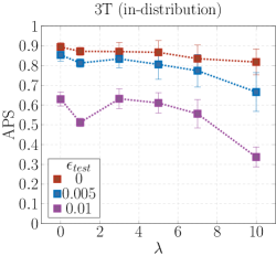
Figure S1: 2D within-distribution performance metrics shown as a function of $\lambda$. Performance is evaluated on benign ($\epsilon_{test}=0$) and disturbed ($\epsilon_{test}>0$) 2D within-distribution (3T) images. All models were trained using $\boldsymbol{\epsilon=0.001}$. As expected, performance generally degraded with increasing disturbance of the test images. Beyond $\lambda=5$, performance on both benign and perturbed samples degrades notably, i.e. strong emphasis on class activation map agreement comes at the cost of a higher misclassification rate. Comparing the model trained under the adversarial regime with the models trained under the interpretability aware regime, we observe that interpretability awareness conveyed a performance advantage on adversarially perturbed 3T images for an optimal choice of $\lambda$, $\lambda\in\{3,5\}$. The advantage becomes more pronounced as the adversary becomes stronger.

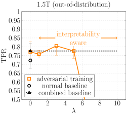
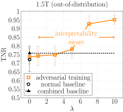
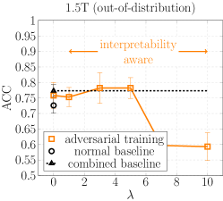
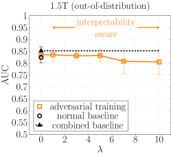
fig:metrics_5_out [TPR]  [TNR]   [ACC]   [AUC]  [APS]

Figure S2: 2D OOD performance metrics shown as a function of $\lambda$. Performance is evaluated on 2D OOD (1.5T) data. Adversarial and interpretability aware models were trained using $\boldsymbol{\epsilon=0.005}$. The ‘normal’ and ‘combined’ baseline indicated by a circle and a triangle are trained on undisturbed data. Models failed to train when $\epsilon_{train}$ was further increased to 0.01. The $\lambda=3$ and $\lambda=5$ interpretability aware models performed better on the unperturbed 1.5T data compared to the adversarial model and the normal baseline. Performance of the best interpretability aware models is on par with that of the combined baseline.

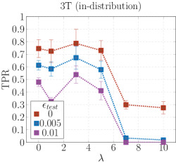
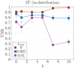
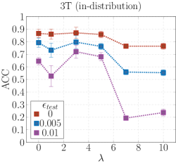
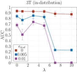
fig:metrics_5_in [TPR]  [TNR]   [ACC]   [AUC]  [APS]

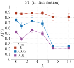
Figure S3: 2D within-distribution performance metrics shown as a function of $\lambda$. Performance is evaluated on benign ($\epsilon_{test}=0$) and disturbed ($\epsilon_{test}>0$) 2D within-distribution (3T) images. All models were trained using $\boldsymbol{\epsilon=0.005}$. Models failed to train when $\epsilon_{train}$ was further increased to 0.01. Interpretability aware models with $\lambda\leq 5$ perform similarly to adversarially trained models on unperturbed 3T test images ($\epsilon_{test}=0$). Performance degrades when $\lambda>5$. Given a strong adversary ($\epsilon_{test}=0.01$), the $\lambda=3$ interpretability aware model outperforms the adversarial model both in terms of TPR and TNR.

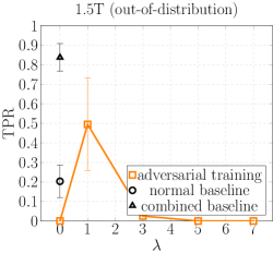
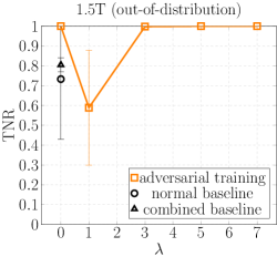
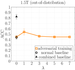
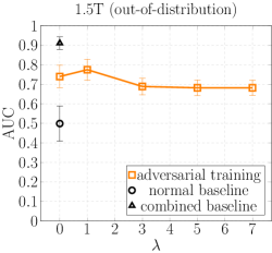
fig:3Dmetrics_out [TPR]  [TNR]   [ACC]   [AUC]   [APS]

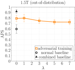
Figure S4: 3D OOD performance metrics shown as a function of $\lambda$. Performance is evaluated on 3D OOD (1.5T) data. Adversarial and interpretability aware models were trained using $\boldsymbol{\epsilon=0.001}$. The ‘normal’ and ‘combined’ baseline indicated by a circle and a triangle are trained on undisturbed data. Interpretability hyperparameters are the same as in the 2D setting and it is likely that a separate hyperparameter optimization procedure would benefit performance.

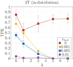
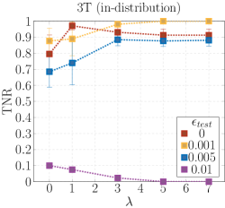
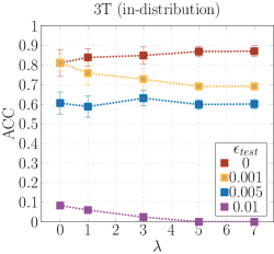
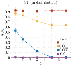
fig:3Dmetrics_in [TPR]   [TNR]   [ACC]   [AUC]   [APS]

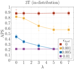
Figure S5: 3D within-distribution performance metrics shown as a function of $\lambda$. Performance is evaluated on benign ($\epsilon_{test}=0$) and disturbed ($\epsilon_{test}>0$) 3D within-distribution (3T) images. All models were trained using $\boldsymbol{\epsilon=0.001}$. Attack and interpretability hyperparameters are the same as in the 2D setting and it is likely that a separate hyperparameter optimization procedure would benefit performance.

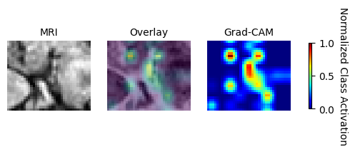
fig:gradcam_tn_c0 [CN subject: CN evidence (int)]   [CN subject: CN evidence (adv)]

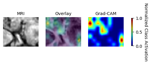
Figure S6: Representative saliency maps of an OOD CN example. Both the adversarial (adv) and the interpretability aware (int) model classified this example correctly. The maps highlight the CN evidence. The saliency map produced by the interpretability aware model highlights brain tissue surrounding the grooves, whereas the adversarial saliency map highlights both tissue and gaps, including features on the edge of the image.

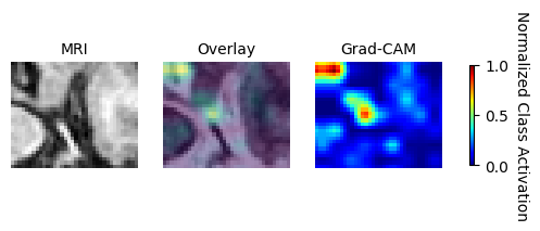
fig:gradcam_ad_c1 [AD patient: AD evidence (int)]   [AD patient: AD evidence (adv)]

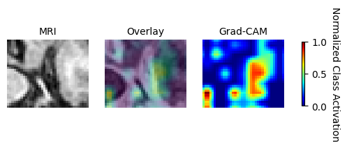
Figure S7: Representative saliency maps of an OOD AD example. Both the adversarial (adv) and the interpretability aware (int) model classified this example correctly. The maps highlight the AD evidence. The saliency map associated with the interpretability aware regime highlights focused regions of brain tissue atrophy, such as the gap in the upper left corner. The adversarial saliency map, on the other hand, highlights a large, unfocused area encompassing brain regions that are not clinically meaningful. Improved model robustness against OOD examples therefore seems to translate to more meaningful explanations, too.

References

- Ahmad et al. (2018) Muhammad Aurangzeb Ahmad, Carly Eckert, and Ankur Teredesai. Interpretable machine learning in healthcare. In Proceedings of the 2018 ACM international conference on bioinformatics, computational biology, and health informatics, pages 559–560, 2018.
- Allen et al. (2019) Bibb Allen, Steven E. Seltzer, Curtis P. Langlotz, Keith P. Dreyer, Ronald M. Summers, Nicholas Petrick, Danica Marinac-Dabic, Marisa Cruz, Tarik K. Alkasab, Robert J. Hanisch, Wendy J. Nilsen, Judy Burleson, Kevin Lyman, and Krishna Kandarpa. A road map for translational research on artificial intelligence in medical imaging: From the 2018 National Institutes of Health/RSNA/ACR/The Academy Workshop. Journal of the American College of Radiology, 16:1179–1189, 2019. 10.1016/j.jacr.2019.04.014.
- Arun et al. (2021) Nishanth Arun, Nathan Gaw, Praveer Singh, Ken Chang, Mehak Aggarwal, Bryan Chen, Katharina Hoebel, Sharut Gupta, Jay Patel, Mishka Gidwani, et al. Assessing the (un) trustworthiness of saliency maps for localizing abnormalities in medical imaging. Radiology: Artificial Intelligence, page e200267, 2021.
- Bloem et al. (2018) Johan L Bloem, Monique Reijnierse, Tom WJ Huizinga, Annette HM van der Helm-van, et al. MR signal intensity: Staying on the bright side in MR image interpretation. RMD Open, 4(1):e000728, 2018.
- Bluemke et al. (2020) David A. Bluemke, Linda Moy, Miriam A. Bredella, Birgit B. Ertl-Wagner, Kathryn J. Fowler, Vicky J. Goh, Elkan F. Halpern, Christopher P. Hess, Mark L. Schiebler, and Clifford R. Weiss. Assessing radiology research on artificial intelligence: A brief guide for authors, reviewers, and readers. Radiology, 294:487–489, 2020. 10.1148/radiol.2019192515.
- Boopathy et al. (2020) Akhilan Boopathy, Sijia Liu, Gaoyuan Zhang, Cynthia Liu, Pin-Yu Chen, Shiyu Chang, and Luca Daniel. Proper network interpretability helps adversarial robustness in classification. In International Conference on Machine Learning (ICML), pages 1014–1023. PMLR, 2020.
- Brüningk et al. (2021) Sarah C Brüningk, Felix Hensel, Louis P Lukas, Merel Kuijs, Catherine R Jutzeler, and Bastian Rieck. Back to the basics with inclusion of clinical domain knowledge-a simple, scalable and effective model of alzheimer’s disease classification. Proceedings of Machine Learning Research, 149:1–24, 2021.
- Carvalho et al. (2019) Diogo V Carvalho, Eduardo M Pereira, and Jaime S Cardoso. Machine learning interpretability: A survey on methods and metrics. Electronics, 8(8):832, 2019.
- Chen et al. (2020) Chen Chen, Wenjia Bai, Rhodri H. Davies, Anish N. Bhuva, Charlotte H. Manisty, Joao B. Augusto, James C Moon, Nay Aung, Aaron M. Lee, Mihir M. Sanghvi, Kenneth Fung, Jose Miguel Paiva, Steffen E. Petersen, Elena Lukaschuk, Stefan K. Piechnik, Stefan Neubauer, and Daniel Rueckert. Improving the generalizability of convolutional neural network-based segmentation on CMR images. Frontiers in Cardiovascular Medicine, 7:105, 2020. 10.3389/fcvm.2020.00105.
- Chen et al. (2018) Pin-Yu Chen, Yash Sharma, Huan Zhang, Jinfeng Yi, and Cho-Jui Hsieh. EAD: Elastic-net attacks to deep neural networks via adversarial examples. In Thirty-Second AAAI Conference on Artificial Intelligence, 2018.
- Duyn et al. (2007) Jeff H Duyn, Peter van Gelderen, Tie-Qiang Li, Jacco A de Zwart, Alan P Koretsky, and Masaki Fukunaga. High-field mri of brain cortical substructure based on signal phase. Proceedings of the National Academy of Sciences, 104(28):11796–11801, 2007.
- Guan et al. (2021) Hao Guan, Li Wang, and Mingxia Liu. Multi-source domain adaptation via optimal transport for brain dementia identification. In 2021 IEEE 18th International Symposium on Biomedical Imaging (ISBI), pages 1514–1517. IEEE, 2021.
- He et al. (2015) Kaiming He, Xiangyu Zhang, Shaoqing Ren, and Jian Sun. Delving deep into rectifiers: Surpassing human-level performance on imagenet classification. Proceedings of the IEEE Conference on Computer Vision and Pattern Recognition (CVPR), pages 1026–1034, 2015.
- Jack et al. (2005) Clifford R Jack, MM Shiung, SD Weigand, PC O’brien, JL Gunter, BF Boeve, DS Knopman, GE Smith, RJ Ivnik, EG Tangalos, et al. Brain atrophy rates predict subsequent clinical conversion in normal elderly and amnestic MCI. Neurology, 65(8):1227–1231, 2005.
- Jack et al. (2008) Clifford R Jack, Matt A Bernstein, Nick C Fox, Paul Thompson, Gene Alexander, Danielle Harvey, Bret Borowski, Paula J Britson, Jennifer L. Whitwell, Chadwick Ward, et al. The Alzheimer’s Disease Neuroimaging Initiative (ADNI): MRI methods. Journal of Magnetic Resonance Imaging: An Official Journal of the International Society for Magnetic Resonance in Medicine, 27(4):685–691, 2008.
- Jiang et al. (2021) Peng-Tao Jiang, Chang-Bin Zhang, Qibin Hou, Ming-Ming Cheng, and Yunchao Wei. LayerCAM: Exploring hierarchical class activation maps for localization. IEEE Transactions on Image Processing, 30:5875–5888, 2021. 10.1109/TIP.2021.3089943.
- Kang et al. (2019) Daniel Kang, Yi Sun, Dan Hendrycks, Tom Brown, and Jacob Steinhardt. Testing robustness against unforeseen adversaries. arXiv preprint arXiv:1908.08016, 2019.
- Knafo (2012) Shira Knafo. Amygdala in Alzheimer’s disease. In Barbara Ferry, editor, The amygdala - A discrete multitasking manager. BoD–Books on Demand, 2012.
- Ladd et al. (2018) Mark E. Ladd, Peter Bachert, Martin Meyerspeer, Ewald Moser, Armin M. Nagel, David G. Norris, Sebastian Schmitter, Oliver Speck, Sina Straub, and Moritz Zaiss. Pros and cons of ultra-high-field MRI/MRS for human application. Progress in Nuclear Magnetic Resonance Spectroscopy, 109:1–50, 2018. https://doi.org/10.1016/j.pnmrs.2018.06.001.
- Lee et al. (2020) Dong-Ho Lee, Yan Li, and Byeong-Seok Shin. Generalization of intensity distribution of medical images using GANs. Human-centric Computing and Information Sciences, 10(1):1–15, 2020.
- Madry et al. (2018) Aleksander Madry, Aleksandar Makelov, Ludwig Schmidt, Dimitris Tsipras, and Adrian Vladu. Towards deep learning models resistant to adversarial attacks. In International Conference on Learning Representations (ICLR), 2018.
- Manera et al. (2020) Ana L Manera, Mahsa Dadar, Vladimir Fonov, and D Louis Collins. CerebrA, registration and manual label correction of Mindboggle-101 atlas for MNI-ICBM152 template. Scientific Data, 7(1):1–9, 2020.
- Mårtensson et al. (2020) Gustav Mårtensson, Daniel Ferreira, Tobias Granberg, Lena Cavallin, Ketil Oppedal, Alessandro Padovani, Irena Rektorova, Laura Bonanni, Matteo Pardini, Milica G Kramberger, et al. The reliability of a deep learning model in clinical out-of-distribution MRI data: A multicohort study. Medical Image Analysis, 66:101714, 2020.
- Rutt and Lee (1996) Brian K Rutt and Donald H Lee. The impact of field strength on image quality in mri. Journal of Magnetic Resonance Imaging, 6(1):57–62, 1996.
- Selvaraju et al. (2017) Ramprasaath R Selvaraju, Michael Cogswell, Abhishek Das, Ramakrishna Vedantam, Devi Parikh, and Dhruv Batra. Grad-cam: Visual explanations from deep networks via gradient-based localization. In 2017 IEEE International Conference on Computer Vision (ICCV), pages 618–626, 2017.
- Zhang et al. (2020) Ling Zhang, Xiaosong Wang, Dong Yang, Thomas Sanford, Stephanie Harmon, Baris Turkbey, Bradford J. Wood, Holger Roth, Andriy Myronenko, Daguang Xu, and Ziyue Xu. Generalizing deep learning for medical image segmentation to unseen domains via deep stacked transformation. IEEE Transactions on Medical Imaging, 39:2531–2540, 2020. 10.1109/TMI.2020.2973595.
- Zhou et al. (2016) Bolei Zhou, Aditya Khosla, Agata Lapedriza, Aude Oliva, and Antonio Torralba. Learning deep features for discriminative localization. Proceedings of the IEEE Conference on Computer Vision and Pattern Recognition (CVPR), pages 2921–2929, 2016.