On algebraically stabilized schemes for convection–diffusion–reaction problems

Abstract

An abstract framework is developed that enables the analysis of algebraically stabilized discretizations in a unified way. This framework is applied to a discretization of this kind for convection–diffusion–reaction equations. The definition of this scheme contains a new limiter that improves a standard one in such a way that local and global discrete maximum principles are satisfied on arbitrary simplicial meshes.

MSC Classification]65N12, 65N30

This work has been supported through the grant No. 19-04243S of the Czech Science Foundation.

1 Introduction

The modeling of physical processes is usually performed on the basis of physical laws, like conservation laws. The derived model is physically consistent if its solutions satisfy the respective laws and, in addition, other important physical properties. Convection–diffusion–reaction equations, which will be considered in this paper, are the result of modeling conservation of scalar quantities, like temperature (energy balance) or concentrations (mass balance). Besides conservation, bounds for the solutions of such equations can be proved (if the data satisfy certain conditions) that reflect physical properties, like non-negativity of concentrations or that the temperature is maximal on the boundary of the body if there are no heat sources and chemical processes inside the body. Such bounds are called maximum principles, e.g., see GT01 . A serious difficulty for computing numerical approximations of solutions of convection–diffusion–reaction equations is that most proposed discretizations do not satisfy the discrete counterpart of the maximum principles, so-called discrete maximum principles (DMPs), and thus they are not physically consistent in this respect. One of the exceptions are algebraically stabilized finite element schemes, e.g., algebraic flux correction (AFC) schemes, where DMPs have been proved rigorously. Methods of this type will be studied in this paper.

The theory developed in this paper is motivated by the numerical solution of the scalar steady-state convection–diffusion–reaction problem

$$-\varepsilon\,\Delta u+{{\boldsymbol{b}}}\cdot\nabla u+c\,u=g\quad\mbox{in $\Omega$}\,,\qquad\qquad u=u_{b}\quad\mbox{on $\partial\Omega$}\,,$$ (1)

where $\Omega\subset{\mathbb{R}}^{d}$, $d\geq 1$, is a bounded domain with a Lipschitz-continuous boundary $\partial\Omega$ that is assumed to be polyhedral (if $d\geq 2$). Furthermore, the diffusion coefficient $\varepsilon>0$ is a constant and the convection field ${{\boldsymbol{b}}}\in W^{1,\infty}(\Omega)^{d}$, the reaction field $c\in L^{\infty}(\Omega)$, the right-hand side $g\in L^{2}(\Omega)$, and the Dirichlet boundary data $u_{b}\in H^{\frac{1}{2}}(\partial\Omega)\cap C(\partial\Omega)$ are given functions satisfying

$$\nabla\cdot{\boldsymbol{b}}=0\,,\qquad c\geq\sigma_{0}\geq 0\qquad\quad\mbox{in $\Omega$}\,,$$ (2)

where $\sigma_{0}$ is a constant.

In applications, one encounters typically the convection-dominated regime, i.e., it is $\varepsilon\ll L\|{\boldsymbol{b}}\|_{0,\infty,\Omega}$, where $L$ is a characteristic length scale of the problem and $\|\cdot\|_{0,\infty,\Omega}$ denotes the norm in $L^{\infty}(\Omega)^{d}$. Then, a characteristic feature of (weak) solutions of (1) is the appearance of layers, which are thin regions where the solution possesses a steep gradient. The thickness of layers is usually (much) below the resolution of the mesh. It is well known that the standard Galerkin finite element method cannot cope with this situation and one has to utilize a so-called stabilized discretization, e.g., see RST08 .

Linear stabilized finite element methods that satisfy DMPs, usually with restrictions to the type of mesh, like the upwind method from BT81 , compute in general very inaccurate results with strongly smeared layers. In order to compute accurate solutions, a nonlinear method has to be applied, typically with parameters that depend on the concrete numerical solution. A nonlinear upwind method was proposed in MH85 and improved in Knobloch06 . In BE05 , a nonlinear edge stabilization method was proposed, see BE02 ; BH04 for related methods, for which a DMP was proved providing that a certain discretization parameter is chosen to be sufficiently large and the mesh is of a certain type. However, already the numerical results presented in BE05 show spurious oscillations. Our own experience from JK08 is that the nonlinear problems for sufficiently large parameters often cannot be solved numerically.

A class of methods that has been developed intensively in recent years is the class of algebraically stabilized schemes, e.g., see BB17 ; BJK17 ; GNPY14 ; Kuzmin06 ; Kuzmin07 ; Kuzmin09 ; Kuzmin12 ; KuzminMoeller05 ; KS17 ; KT04 ; LKSM17 . The origins of this approach can be tracked back to BorisBook73 ; Zalesak79 . In these schemes, the stabilization is performed on the basis of the algebraic system of equations obtained with the Galerkin finite element method. Then, so-called limiters are computed, which maintain the conservation property and which restrict the stabilized discretization mainly to a vicinity of layers to ensure the satisfaction of DMPs without compromising the accuracy. There are several limiters proposed in the literature, like the so-called Kuzmin Kuzmin07 , BJK BJK17 , or BBK BBK17 limiters. Both, the Kuzmin and the BBK limiters were utilized in BBK17a for defining a scheme that blends a standard linear stabilized scheme in smooth regions and a nonlinear stabilized method in a vicinity of layers.

An advantage of algebraically stabilized schemes is that they satisfy a DMP by construction, often under some assumptions on the mesh, and they usually provide sharp approximations of layers, cf. the numerical results in, e.g., ACF+11 ; GKT12 ; JS08 ; Kuzmin12 . In numerical studies presented in JJ19 , it turned out that the results with the BJK limiter were usually more accurate than with the Kuzmin limiter, if the nonlinear problems for the BJK limiter could be solved. However, solving these problems was often not possible for strongly convection-dominated cases. Numerical studies in BJK18 show that using the Kuzmin limiter leads to solutions with sharper layers compared with the solutions obtained with the BBK limiter. As a consequence of these experiences, it seems to be advisable from the point of view of applications to use algebraically stabilized schemes on the basis of the Kuzmin limiter. The AFC scheme with the Kuzmin limiter was analyzed in BJK16 , thereby proving the existence of a solution, the satisfaction of a local DMP, and an error estimate. The local DMP requires lumping the reaction term and using certain types of meshes, e.g., Delaunay meshes in two dimensions, analogously as for the methods from BBK17 ; BBK17a .

The conservation and stability properties of algebraically stabilized schemes are given if the added stabilization is a symmetric term. For many schemes, this term consists of two factors, an artificial diffusion matrix and the matrix of the limiters, and usually the methods are constructed in such a way that both factors are symmetric. Only recently, motivated by BB17 , a more general approach where only the product is symmetric but not the individual factors was considered in Kno21 .

The first main goal of this paper is the development of an abstract framework that allows to analyze algebraically stabilized discretizations in a unified way. Although our main interest is the numerical solution of problem (1), many considerations will be more general and then problem (1) and its discretizations will only serve as a motivation for our assumptions. Hence, this framework covers a larger class of algebraically stabilized discretizations than the available analysis.

The second main goal consists in proposing and analyzing a modification of the Kuzmin limiter such that, if applied in the framework of the algebraic stabilization of Kno21 , the positive features of the AFC method with the Kuzmin limiter are preserved on meshes where it works well and, in addition, local and global DMPs can be proved on arbitrary simplicial meshes. In particular, our intention was to preserve the upwind character of the AFC method with the Kuzmin limiter. There are already proposals in this direction in the framework of AFC methods. In Kno17 , the Kuzmin limiter is replaced in cases where it does not lead to the validity of the local DMP in a somewhat ad hoc way by a value that introduces more artificial diffusion. The satisfaction of the local DMP on arbitrary simplicial meshes could be proved for this approach. Whether or not the assumption for the existence of a solution of the nonlinear problem is satisfied with this limiter is not discussed. A combination of the Kuzmin and the BJK limiters to obtain a limiter of upwind type for which the AFC scheme satisfies a local DMP on arbitrary simplicial meshes and is linearity preserving is proposed in Kno19 . The definition of this limiter is closer to the BJK than to the Kuzmin limiter. As already mentioned, in Kno21 , a new algebraically stabilized method was proposed that does not require the symmetry of the limiter. Initial numerical results for a nonsymmetric modification of the Kuzmin limiter are presented in Kno21 , but a numerical analysis is missing. The abstract framework mentioned in the previous paragraph covers in particular the method from Kno21 .

In the present paper, the limiter from Kno21 is written in a simpler form, without using internodal fluxes typical for AFC methods. Moreover, a novel modification is performed that improves the accuracy in some computations using non-Delaunay meshes. Of course, this modification is performed in such a way that the resulting method still fits in the abstract analytic framework. The definition of the new method does not contain any ambiguity, in contrast to the AFC method with Kuzmin limiter, which is not uniquely defined in some cases (cf. Remark 8 in BJK16 ). A further advantage of the considered approach is that, in contrast to the AFC method with Kuzmin limiter, lumping of the reaction term is no longer necessary for the satisfaction of the DMP, which enables to obtain sharper layers as we will demonstrate by numerical results.

This paper is organized as follows. Sect. 2 introduces the basic discretization of (1) and its algebraic form. An abstract framework for an algebraic stabilization is presented in Sect. 3. The following section studies the solvability and the satisfaction of local and global DMPs for the abstract algebraic stabilization and Sect. 5 provides an error analysis. In Sect. 6, the AFC scheme with Kuzmin limiter as an example of algebraic stabilization from Sect. 3 is presented, its properties are discussed for the discretizations from Sect. 2 and the definition of the limiter is reformulated. The reformulation is utilized in Sect. 7 for proposing a new limiter such that the resulting algebraically stabilized scheme is of upwind type and satisfies DMPs on arbitrary simplicial meshes. Sect. 8 presents numerical examples which show that the algebraically stabilized scheme with the new limiter in fact cures the deficiencies of the AFC scheme with Kuzmin limiter.

2 The convection–diffusion–reaction problem and its finite element discretization

The weak solution of the convection–diffusion–reaction problem (1) is a function $u\in H^{1}(\Omega)$ satisfying the boundary condition $u=u_{b}$ on $\partial\Omega$ and the variational equation

$$a(u,v)=(g,v)\qquad\forall\,\,v\in H^{1}_{0}(\Omega)\,,$$

where

$$a(u,v)=\varepsilon\,(\nabla u,\nabla v)+({{\boldsymbol{b}}}\cdot\nabla u,v)+(c\,u,v)\,.$$ (3)

As usual, $(\cdot,\cdot)$ denotes the inner product in $L^{2}(\Omega)$ or $L^{2}(\Omega)^{d}$. It is well known that the weak solution of (1) exists and is unique (cf. Evans ).

An important property of problem (1) is that, for $c\geq 0$ in $\Omega$, its solutions satisfy the maximum principle. The classical maximum principle (cf. Evans ) states the following: if $u\in C^{2}(\Omega)\cap C(\overline{\Omega})$ solves (1) and the functions ${\boldsymbol{b}}$ and $c$ are bounded in $\Omega$, then, for any set $G\subset\overline{\Omega}$, one has the implications

$$g\leq 0\quad\mbox{\rm in}\,\,\,G\qquad\Rightarrow\qquad\max_{\overline{G}}\,u\leq\max_{\partial G}\,u^{+}\,,$$ (4)

$$g\geq 0\quad\mbox{\rm in}\,\,\,G\qquad\Rightarrow\qquad\min_{\overline{G}}\,u\geq\min_{\partial G}\,u^{-}\,,$$ (5)

where $u^{+}=\max\{u,0\}$, $u^{-}=\min\{u,0\}$. If, in addition, $c=0$ in $G$, then

$$g\leq 0\quad\mbox{\rm in}\,\,\,G\qquad\Rightarrow\qquad\max_{\overline{G}}\,u=\max_{\partial G}\,u\,,$$ (6)

$$g\geq 0\quad\mbox{\rm in}\,\,\,G\qquad\Rightarrow\qquad\min_{\overline{G}}\,u=\min_{\partial G}\,u\,.$$ (7)

Analogous statements also hold for the weak solutions, cf. GT01 .

To define a finite element discretization of problem (1), we consider a simplicial triangulation ${\mathscr{T}}_{h}$ of $\overline{\Omega}$ which is assumed to belong to a regular family of triangulations in the sense of Ciarlet . Furthermore, we introduce finite element spaces

$$W_{h}=\{v_{h}\in C(\overline{\Omega})\,\mathchar 24635\relax\;\,\,v_{h}|_{T}\in\mathbb{P}_{1}(T)\,\,\forall\,T\in{\mathscr{T}}_{h}\}\,,\qquad V_{h}=W_{h}\cap H^{1}_{0}(\Omega)\,,$$

consisting of continuous piecewise linear functions. The vertices of the triangulation ${\mathscr{T}}_{h}$ will be denoted by $x_{1},\dots,x_{N}$ and we assume that $x_{1},\dots,x_{M}\in\Omega$ and $x_{M+1},\dots,x_{N}\in\partial\Omega$. Then the usual basis functions $\varphi_{1},\dots,\varphi_{N}$ of $W_{h}$ are defined by the conditions $\varphi_{i}(x_{j})=\delta_{ij}$, $i,j=1,\dots,N$, where $\delta_{ij}$ is the Kronecker symbol. Obviously, the functions $\varphi_{1},\dots,\varphi_{M}$ form a basis of $V_{h}$. Any function $u_{h}\in W_{h}$ can be written in a unique way in the form

$$u_{h}=\sum_{i=1}^{N}u_{i}\,\varphi_{i}$$ (8)

and hence it can be identified with the coefficient vector ${\rm U}=(u_{1},\dots,u_{N})$.

Now an approximate solution of problem (1) can be introduced as the solution of the following finite-dimensional problem:

Find $u_{h}\in W_{h}$ such that $u_{h}(x_{i})=u_{b}(x_{i})$, $i=M+1,\dots,N$, and

$$a_{h}(u_{h},v_{h})=(g,v_{h})\qquad\forall\,\,v_{h}\in V_{h}\,,$$ (9)

where $a_{h}$ is a bilinear form approximating the bilinear form $a$. In particular, one can use $a_{h}=a$. Another possibility is to set

$$a_{h}(u_{h},v_{h})=\varepsilon\,(\nabla u_{h},\nabla v_{h})+({{\boldsymbol{b}}}\cdot\nabla u_{h},v_{h})+\sum_{i=1}^{M}\,(c,\varphi_{i})\,u_{i}\,v_{i}$$ (10)

for any $u_{h}\in W_{h}$ and $v_{h}\in V_{h}$, i.e., to consider a lumping of the reaction term $(c\,u_{h},v_{h})$ in $a(u_{h},v_{h})$. This may help to satisfy the DMP for problem (9), cf. Sect. 6. We assume that $a_{h}$ is elliptic on the space $V_{h}$, i.e., there is a constant $C_{a}>0$ such that

$$a_{h}(v_{h},v_{h})\geq C_{a}\,\|v_{h}\|_{a}^{2}\qquad\forall\,\,v_{h}\in V_{h}\,,$$ (11)

where $\|\cdot\|_{a}$ is a norm on the space $H^{1}_{0}(\Omega)$ but generally only a seminorm on the space $H^{1}(\Omega)$. This guarantees that the discrete problem (9) has a unique solution. In view of (2), the ellipticity condition (11) holds for both $a_{h}=a$ and $a_{h}$ defined by (10) with $C_{a}=1$ and

$$\|v\|_{a}^{2}=\varepsilon\,|v|_{1,\Omega}^{2}+\sigma_{0}\,\|v\|_{0,\Omega}^{2}\,.$$ (12)

We denote

$$a_{ij} =a_{h}(\varphi_{j},\varphi_{i})\,,\qquad i,j=1,\dots,N\,,$$ (13)

$$g_{i} =(g,\varphi_{i})\,,\qquad i=1,\dots,M\,,$$ (14)

$$u^{b}_{i} =u_{b}(x_{i})\,,\qquad i=M+1,\dots,N\,.$$ (15)

Then $u_{h}$ is a solution of the finite-dimensional problem (9) if and only if the coefficient vector $(u_{1},\dots,u_{N})$ corresponding to $u_{h}$ satisfies the algebraic problem

$$\sum_{j=1}^{N}\,a_{ij}\,u_{j}=g_{i}\,,\qquad i=1,\dots,M\,,$$

$$u_{i}=u^{b}_{i}\,,\qquad i=M+1,\dots,N\,.$$

As discussed in the introduction, the above discretizations are not appropriate in the convection-dominated regime and a stabilization has to be applied. In the next sections, algebraic stabilization techniques will be studied. As already mentioned, a general framework will be presented and the numerical solution of convection–diffusion–reaction equations serves just as a motivation for the assumptions.

3 An abstract framework

In this section we assume that we are given a system of linear algebraic equations of the form

$$\sum_{j=1}^{N}\,a_{ij}\,u_{j}=g_{i}\,,\qquad i=1,\dots,M\,,$$ (16)

$$u_{i}=u^{b}_{i}\,,\qquad i=M+1,\dots,N\,,$$ (17)

(with $0<M<N$) corresponding to a discretization of a linear boundary value problem for which the maximum principle holds. An example is the algebraic problem derived in the preceding section.

We assume that the row sums of the system matrix are nonnegative, i.e.,

$$\sum_{j=1}^{N}\,a_{ij}\geq 0\,,\qquad\quad i=1,\dots,M\,,$$ (18)

and that the submatrix $(a_{ij})_{i,j=1}^{M}$ is positive definite, i.e.,

$$\sum_{i,j=1}^{M}\,u_{i}\,a_{ij}\,u_{j}>0\qquad\forall\,\,(u_{1},\dots,u_{M})\in{\mathbb{R}}^{M}\setminus\{0\}\,.$$ (19)

For the discretizations from the previous section, the latter property follows from (11), whereas (18) is a consequence of the nonnegativity of $c$ and the fact that $\sum_{j=1}^{N}\varphi_{j}=1$.

Since the algebraic problem (16), (17) is assumed to approximate a problem satisfying the maximum principle, it is natural to require that an analog of this property also holds in the discrete case, at least locally. Then an important physical property of the original problem will be preserved and spurious oscillations of the approximate solution will be excluded. To formulate a local DMP, we have to specify a neighborhood

$$S_{i}\subset\{1,\dots,N\}\setminus\{i\}$$

of any $i\in\{1,\dots,M\}$ (i.e., of any interior vertex $x_{i}$ if the geometric interpretation from the previous section is considered). For example, one can set

$$S_{i}=\{j\in\{1,\dots,N\}\setminus\{i\}\,\mathchar 24635\relax\;\,\,a_{ij}\neq 0\}\,,\qquad i=1,\dots,M\,.$$ (20)

Then, under the assumptions (18) and (19), the solution of (16), (17) satisfies the local DMP

$$g_{i}\leq 0\quad\Rightarrow\quad u_{i}\leq\max_{j\in S_{i}}\,u_{j}^{+}\,,\qquad\qquad g_{i}\geq 0\quad\Rightarrow\quad u_{i}\geq\min_{j\in S_{i}}\,u_{j}^{-}$$ (21)

(with any $i\in\{1,\dots,M\}$) if and only if (cf. (BJK16, , Lemma 21))

$$a_{ij}\leq 0\qquad\forall\,\,i\neq j,\,i=1,\dots,M,\,j=1,\dots,N\,.$$ (22)

Moreover, the stronger local DMP

$$g_{i}\leq 0\quad\Rightarrow\quad u_{i}\leq\max_{j\in S_{i}}\,u_{j}\,,\qquad\qquad g_{i}\geq 0\quad\Rightarrow\quad u_{i}\geq\min_{j\in S_{i}}\,u_{j}$$ (23)

holds (again with any $i\in\{1,\dots,M\}$) if and only if the conditions (22) and

$$\sum_{j=1}^{N}\,a_{ij}=0\,,\qquad\quad i=1,\dots,M\,,$$ (24)

are satisfied (cf. (BJK16, , Lemma 22)). For the discretizations from the previous section, (24) holds if $c=0$ in $\Omega$, which is a condition used for proving (6) and (7), i.e., a counterpart of (23).

In many cases, the condition (22) is violated (like for the discretizations from the previous section in the convection-dominated regime) and hence the local DMPs (21) and (23) do not hold. To enforce the DMP, one can add a sufficient amount of artificial diffusion to (16), e.g., in the following way. First, the system matrix is extended to a matrix ${\mathbb{A}}=(a_{ij})_{i,j=1}^{N}$, typically using the matrix corresponding to the underlying discretization in the case when homogeneous natural boundary conditions are used instead of the Dirichlet ones (i.e., using (13) if the setting of the previous section is considered). Then one can define a symmetric artificial diffusion matrix $\mathbb{D}=(d_{ij})_{i,j=1}^{N}$ possessing the entries

$$d_{ij}=d_{ji}=-\max\{a_{ij},0,a_{ji}\}\qquad\forall\,\,i\neq j\,,\qquad\qquad d_{ii}=-\sum_{j\neq i}\,d_{ij}\,.$$ (25)

The matrix $\mathbb{D}$ has zero row and column sums and is positive semidefinite (cf. (BJK16, , Lemma 1)), the matrix ${\mathbb{A}}+{\mathbb{D}}$ has nonpositive off-diagonal entries by construction and the submatrix $(a_{ij}+d_{ij})_{i,j=1}^{M}$ is positive definite. Consequently, the stabilized algebraic problem

$$\sum_{j=1}^{N}\,(a_{ij}+d_{ij})\,u_{j}=g_{i}\,,\qquad i=1,\dots,M\,,$$ (26)

$$u_{i}=u^{b}_{i}\,,\qquad i=M+1,\dots,N\,,$$ (27)

is uniquely solvable and its solution satisfies the local DMP (21) with

$$S_{i}=\{j\in\{1,\dots,N\}\setminus\{i\}\,\mathchar 24635\relax\;\,\,a_{ij}\neq 0\,\,\,\mbox{or}\,\,\,a_{ji}>0\}\,,\qquad i=1,\dots,M\,.$$ (28)

If the condition (24) holds, then the solution of (26), (27) also satisfies the stronger local DMP (23), again with $S_{i}$ defined by (28). Moreover, if the above stabilization is applied to the discretizations from the previous section, then, for weakly acute triangulations, the approximate solutions converge to the solution of (1), see BJK16 .

However, the amount of artificial diffusion added in (26) is usually too large and leads to an excessive smearing of layers if it is applied to stabilize discretizations of (1) in the convection-dominated regime. To suppress the smearing, the artificial diffusion should be added mainly in regions where the solution changes abruptly and hence it should depend on the unknown approximate solution ${\rm U}=(u_{1},\dots,u_{N})$. This motivates us to introduce a general artificial diffusion matrix ${\mathbb{B}}({\rm U})=(b_{ij}({\rm U}))_{i,j=1}^{N}$ having analogous properties as the matrix ${\mathbb{D}}$, i.e., for any ${\rm U}\in{\mathbb{R}}^{N}$, we assume that

$$b_{ij}({\rm U})=b_{ji}({\rm U})\,,\qquad\quad i,j=1,\dots,N\,,$$ (29)

$$b_{ij}({\rm U})\leq 0,\qquad\quad i,j=1,\dots,N\,,\,\,i\neq j\,,$$ (30)

$$\sum_{j=1}^{N}\,b_{ij}({\rm U})=0\,,\qquad\quad i=1,\dots,N\,.$$ (31)

Like above, we introduce local index sets $S_{i}$ such that

$$\{j\in\{1,\dots,N\}\setminus\{i\}\,\mathchar 24635\relax\;\,\,a_{ij}\neq 0\}\subset S_{i}\subset\{1,\dots,N\}\setminus\{i\}\,,\quad i=1,\dots,M\,,$$ (32)

and, for any ${\rm U}\in{\mathbb{R}}^{N}$,

$$b_{ij}({\rm U})=0\qquad\forall\,\,j\not\in S_{i}\cup\{i\},\,i=1,\dots,M\,.$$ (33)

Let us mention that if the algebraic problem (16), (17) corresponds to a finite element discretization based on piecewise linear functions as in the preceding section, one can usually use index sets

$$S_{i}=\{j\in\{1,\dots,N\}\setminus\{i\}\,\mathchar 24635\relax\;\,\,\mbox{\rm$x_{i}$ and $x_{j}$ are end points of the same edge}\}\,,$$ (34)

$i=1,\dots,M$, where $x_{1},\dots,x_{N}$ are the vertices of the underlying simplicial triangulation, numbered as in the preceding section.

Now, we consider the nonlinear algebraic problem

$$\sum_{j=1}^{N}\,(a_{ij}+b_{ij}({\rm U}))\,u_{j}=g_{i}\,,\qquad i=1,\dots,M\,,$$ (35)

$$u_{i}=u^{b}_{i}\,,\qquad i=M+1,\dots,N\,.$$ (36)

Note that, in view of (31) and (33), system (35) can be written in the form

$$\sum_{j=1}^{N}\,a_{ij}\,u_{j}+\sum_{j\in S_{i}}\,b_{ij}({\rm U})\,(u_{j}-u_{i})=g_{i}\,,\qquad i=1,\dots,M\,.$$ (37)

In view of (29) and (30), one obtains the important property (cf. (BJK16, , Lemma 1))

$$\sum_{i,j=1}^{N}\,v_{i}\,b_{ij}({\rm U})\,(v_{j}-v_{i})=-\frac{1}{2}\,\sum_{i,j=1}^{N}\,b_{ij}({\rm U})\,(v_{j}-v_{i})^{2}\geq 0\qquad\forall\,\,{\rm U},{\rm V}\in{\mathbb{R}}^{N}\,.$$ (38)

Thus, due to (31), the matrix ${\mathbb{B}}({\rm U})$ is positive semidefinite for any ${\rm U}\in{\mathbb{R}}^{N}$.

4 Analysis of the abstract nonlinear algebraic problem

The aim of this section is to investigate the solvability and the validity of the DMP for the nonlinear algebraic problem (35), (36). These investigations will generalize the results obtained in BJK16 ; Kno17 ; BJK18 .

To prove the solvability of the system (35), (36), we make the following assumption.

Assumption (A1): For any $i\in\{1,\dots,M\}$ and any $j\in\{1,\dots,N\}$, the function $b_{ij}({\rm U})(u_{j}-u_{i})$ is a continuous function of ${\rm U}=(u_{1},\dots,u_{N})\in{\mathbb{R}}^{N}$ and, for any $i\in\{1,\dots,M\}$ and any $j\in\{M+1,\dots,N\}$, the function $b_{ij}({\rm U})$ is a bounded function of ${\rm U}\in{\mathbb{R}}^{N}$.

Theorem 1.

Let (19) and (29)–(31) hold and let Assumption (A1) be satisfied. Then there exists a solution of the nonlinear problem (35), (36).

Proof: The proof follows the lines of the proof of Theorem 3 in BJK16 . We denote by $\widetilde{\rm V}\equiv(v_{1},\dots,v_{M})$ the elements of the space ${\mathbb{R}}^{M}$ and, if $v_{i}$ with $i\in\{M+1,\dots,N\}$ occurs, we assume that $v_{i}=u^{b}_{i}$. To any $\widetilde{\rm V}\in{\mathbb{R}}^{M}$, we assign ${\rm V}:=(v_{1},\dots,v_{N})$. Let us define the operator $T:{\mathbb{R}}^{M}\to{\mathbb{R}}^{M}$ by

$$(T\,\widetilde{\rm V})_{i}=\sum_{j=1}^{N}\,a_{ij}\,v_{j}+\sum_{j=1}^{N}\,b_{ij}({\rm V})\,(v_{j}-v_{i})-g_{i}\,,\qquad i=1,\dots,M\,.$$

Then ${\rm U}$ is a solution of the nonlinear problem (35), (36) if and only if $T\,\widetilde{\rm U}=0$. The operator $T$ is continuous and, in view of (19) and (38), there exist constants $C_{1}$, $C_{2}>0$ such that (cf. (BJK16, , Theorem 3) for details)

$$(T\,\widetilde{\rm V},\widetilde{\rm V})\geq C_{1}\,\|\widetilde{\rm V}\|^{2}-C_{2}\qquad\forall\,\,\widetilde{\rm V}\in{\mathbb{R}}^{M}\,,$$

where $(\cdot,\cdot)$ is the usual inner product in ${\mathbb{R}}^{M}$ and $\|\cdot\|$ the corresponding (Euclidean) norm. Then, for any $\widetilde{\rm V}\in{\mathbb{R}}^{M}$ satisfying $\|\widetilde{\rm V}\|=\sqrt{2\,C_{2}/C_{1}}$, one has $(T\,\widetilde{\rm V},\widetilde{\rm V})>0$ and hence it follows from Brouwer’s fixed-point theorem (see (Temam77, , p. 164, Lemma 1.4)) that there exists $\widetilde{\rm U}\in{\mathbb{R}}^{M}$ such that $T\,\widetilde{\rm U}=0$.

Remark 1.

For proving the solvability of (35), (36), it would be sufficient to assume that the functions $b_{ij}({\rm U})u_{j}$ are continuous. However, since $b_{ij}({\rm U})$ should depend on local variations of $\rm U$ with respect to $u_{i}$, the assumed continuity of $b_{ij}({\rm U})(u_{j}-u_{i})$ is more useful. The functions $b_{ij}({\rm U})$ themselves are often not continuous, cf. Remark 7.

Remark 2.

The solution of (35), (36) is unique if ${\mathbb{B}}({\rm U})\rm U$ is Lipschitz–continuous with a sufficiently small constant. As pointed out in Lohman19 , this condition can be further refined by introducing a positive semidefinite matrix $\mathbb{D}$, e.g., the one defined in (25), and investigating the Lipschitz continuity of $({\mathbb{B}}({\rm U})-\mathbb{D}){\rm U}$. Since, in view of (19), there is $C>0$ such that

$$C\,\|{\rm V}\|\leq\|(\mathbb{A}+\mathbb{D}){\rm V}\|\qquad\forall\,\,{\rm V}\in{\mathbb{R}}^{N},v_{M+1}=\dots=v_{N}=0\,,$$

($\|\cdot\|$ is again the Euclidean norm on ${\mathbb{R}}^{M}$), the smallness assumption on the Lipschitz constant can be expressed by the inequality

$$\|({\mathbb{B}}({\rm U})-\mathbb{D}){\rm U}-({\mathbb{B}}({\rm V})-\mathbb{D}){\rm V}\|<\|(\mathbb{A}+\mathbb{D})({\rm U-V})\|$$

$$\hskip 56.9055pt\forall\,\,{\rm U}\neq{\rm V}\in{\mathbb{R}}^{N}\,\,\,\mbox{\rm with}\,\,\,(u_{M+1},\dots,u_{N})=(v_{M+1},\dots,v_{N})\,.$$ (39)

Then, if ${\rm U}\neq\overline{\rm U}$ are two solutions of (35), (36), one has

$$[(\mathbb{A}+{\mathbb{B}}({\rm U})){\rm U}]_{i}=[(\mathbb{A}+{\mathbb{B}}(\overline{\rm U}))\overline{\rm U}]_{i},\qquad i=1,\dots,M\,,$$

and (39) leads to a contradiction. Nevertheless, the inequality (39) is often not satisfied and then the uniqueness of the nonlinear problem (35), (36) is open.

Now let us investigate the validity of DMPs for problem (35), (36). To this end, one has to relate the properties of the artificial diffusion matrix ${\mathbb{B}}({\rm U})$ to the matrix ${\mathbb{A}}$. This can be done in various ways and we shall use the following assumption that generalizes the one used in Kno17 .

Assumption (A2): Consider any ${\rm U}=(u_{1},\dots,u_{N})\in\mathbb{R}^{N}$ and any $i\in\{1,\dots,M\}$. If $u_{i}$ is a strict local extremum of $\rm U$ with respect to $S_{i}$ from (32), (33), i.e.,

$$u_{i}>u_{j}\quad\forall\,\,j\in S_{i}\qquad\mbox{or}\qquad u_{i}<u_{j}\quad\forall\,\,j\in S_{i}\,,$$

then

$$a_{ij}+b_{ij}({\rm U})\leq 0\qquad\forall\,\,j\in S_{i}\,.$$

Remark 3.

In contrast to linear problems, it is only assumed that off-diagonal entries of the matrix ${\mathbb{A}}+{\mathbb{B}}({\rm U})$ are nonpositive in rows corresponding to indices where strict local extrema of $\rm U$ appear. If ${\mathbb{B}}$ does not depend on $\rm U$, then Assumption (A2) implies that the first $M$ rows of ${\mathbb{A}}+{\mathbb{B}}$ have nonpositive off-diagonal entries, which is a necessary and sufficient condition for the validity of the local DMP under our assumptions on ${\mathbb{A}}$ and ${\mathbb{B}}$.

Theorem 2.

Let (18), (19), and (29)–(33) hold and let Assumption (A2) be satisfied. Then any solution ${\rm U}=(u_{1},\dots,u_{N})\in\mathbb{R}^{N}$ of (35) satisfies the local DMP (21) for all $i=1,\dots,M$. If condition (24) holds, then the stronger local DMP (23) is also valid.

Proof: The proof is basically the same as in Kno17 . Since it is short, we repeat it for completeness. Let ${\rm U}=(u_{1},\dots,u_{N})\in\mathbb{R}^{N}$ satisfy (35). Consider any $i\in\{1,\dots,M\}$ and let $g_{i}\leq 0$. Denoting $A_{i}=\sum_{j=1}^{N}a_{ij}$, it follows from (37) that

$$A_{i}\,u_{i}+\sum_{j\in S_{i}}\,[a_{ij}+b_{ij}({\rm U})]\,(u_{j}-u_{i})=g_{i}\,.$$ (40)

If $A_{i}>0$, we want to prove the first implication in (21) for which it suffices to consider $u_{i}>0$ since otherwise the implication trivially holds. If $A_{i}=0$, an arbitrary sign of $u_{i}$ is considered. Let us assume that $u_{i}>u_{j}$ for all $j\in S_{i}$. Then Assumption (A2) implies that each term of the sum in (40) is nonnegative. If $A_{i}=0$, then there is $j\in S_{i}$ such that $a_{ij}<0$ since $a_{ii}>0$ (see (19)). This together with (30) implies that the sum in (40) is positive. If $A_{i}>0$, then $A_{i}\,u_{i}>0$. Thus, in both cases, the left-hand side of (40) is positive, which is a contradiction. Therefore, there is $j\in S_{i}$ such that $u_{i}\leq u_{j}$, which proves the first implication in (23) and hence also in (21). The statements for $g_{i}\geq 0$ follow in an analogous way.

Our next aim will be to show that, under the above assumptions, also a global DMP is satisfied. First we prove the following general form of the DMP, which generalizes a result proved in BJK18 .

Theorem 3.

Let (18), (19), and (29)–(33) hold and let Assumptions (A1) and (A2) be satisfied. Consider any nonempty set $R\subset\{1,\dots,M\}$ and denote

$$P:=R\cup\bigcup_{i\in R}\,S_{i}\,,\qquad Q:=P\setminus R\,.$$ (41)

Assume that $Q\neq\emptyset$. Then any solution ${\rm U}=(u_{1},\dots,u_{N})\in\mathbb{R}^{N}$ of (35) satisfies the DMP

$$g_{i}\leq 0\quad\forall\,\,i\in R\qquad\Rightarrow\qquad\max_{i\in P}u_{i}\leq\max_{i\in Q}\,u_{i}^{+}\,,$$ (42)

$$g_{i}\geq 0\quad\forall\,\,i\in R\qquad\Rightarrow\qquad\min_{i\in P}u_{i}\geq\min_{i\in Q}\,u_{i}^{-}\,.$$ (43)

If, in addition,

$$\sum_{j=1}^{N}\,a_{ij}=0\quad\,\,\quad\forall\,\,i\in R\,,$$ (44)

then

$$g_{i}\leq 0\quad\forall\,\,i\in R\qquad\Rightarrow\qquad\max_{i\in P}u_{i}=\max_{i\in Q}\,u_{i}\,,$$ (45)

$$g_{i}\geq 0\quad\forall\,\,i\in R\qquad\Rightarrow\qquad\min_{i\in P}u_{i}=\min_{i\in Q}\,u_{i}\,.$$ (46)

Proof: The proof is based on the technique used in (Kno10, , Theorems 5.1 and 5.2). Let ${\rm U}=(u_{1},\dots,u_{N})$ satisfy (35) and let $g_{i}\leq 0$ for all $i\in R$. We denote

$$\widetilde{a}_{ij}:=a_{ij}+b_{ij}({\rm U})\,,\qquad i=1,\dots,M,\,\,j=1,\dots,N\,.$$

Then, according to (31)–(33), (18), (38), (19) and (35), one has

$$\sum_{j\in P}\,\widetilde{a}_{ij}=\sum_{j=1}^{N}\,a_{ij}\geq 0\qquad\forall\,\,i\in R\,,$$ (47)

$$\sum_{i,j=1}^{M}\,v_{i}\,\widetilde{a}_{ij}\,v_{j}\geq\sum_{i,j=1}^{M}\,v_{i}\,a_{ij}\,v_{j}>0\qquad\forall\,\,(v_{1},\dots,v_{M})\in{\mathbb{R}}^{M}\setminus\{0\}\,,$$ (48)

$$\sum_{j\in P}\,\widetilde{a}_{ij}\,u_{j}=g_{i}\qquad\forall\,\,i\in R\,.$$ (49)

Denote

$$s=\max\{u_{i}\,\mathchar 24635\relax\;\,\,i\in P\}\,,\qquad J=\{i\in P\,\mathchar 24635\relax\;\,\,u_{i}=s\}\,.$$

It suffices to consider the case $J\neq P$ since otherwise the validity of (42) and (45) is obvious. First, let us show that

$$\widetilde{a}_{ij}\leq 0\qquad\forall\,\,i\in J\cap R,\,\,j\in P\setminus J\,.$$ (50)

Let $i\in J\cap R$ and $j\in S_{i}\setminus J$. For any $k\in\mathbb{N}$, define the vector ${\rm U}^{k}=(u_{1}^{k},\dots,u_{N}^{k})$ with $u_{i}^{k}=u_{i}+1/k$ and $u_{l}^{k}=u_{l}$ for $l\neq i$. Then $u^{k}_{i}$ is a strict local maximum of ${\rm U}^{k}$ with respect to $S_{i}$ and hence, in view of Assumption (A2),

$$(a_{ij}+b_{ij}({\rm U}^{k}))\,(u^{k}_{i}-u^{k}_{j})\leq 0\,.$$

Since ${\rm U}^{k}\to{\rm U}$ for $k\to\infty$, Assumption (A1) implies that

$$(a_{ij}+b_{ij}({\rm U}))\,(u_{i}-u_{j})\leq 0\,.$$

As $u_{i}-u_{j}>0$, it follows that $a_{ij}+b_{ij}({\rm U})\leq 0$. For $j\not\in S_{i}\cup\{i\}$, one has $a_{ij}+b_{ij}({\rm U})=0$, which completes the proof of (50).

Now we want to prove that the relations (47)–(50) imply (42) and (45). If (44) does not hold, it suffices to consider $s>0$ since otherwise (42) trivially holds. Let us assume that (45) does not hold, which implies that $J\subset R$. We shall prove that then

$$\exists\,\,k\in J:\quad\mu_{k}:=\sum_{j\in J}\,\widetilde{a}_{kj}>0\,.$$ (51)

Assume that (51) is not satisfied. Then, applying (47) and (50), one derives for any $i\in J$

$$0\geq\sum_{j\in J}\,\widetilde{a}_{ij}\geq-\sum_{j\in P\setminus J}\,\widetilde{a}_{ij}\geq 0\,,$$

which gives

$$\sum_{j\in J}\,\widetilde{a}_{ij}=0\qquad\forall\,\,i\in J\,.$$

Thus, the matrix $(\widetilde{a}_{ij})_{i,j\in J}$ is singular, which contradicts (48). Therefore, (51) holds and hence, denoting $r=\max\{u_{i}\,\mathchar 24635\relax\;\,\,i\in P\setminus J\}\,,$ one obtains using (49) and (50)

$$s\,\mu_{k}=\sum_{j\in J}\,\widetilde{a}_{kj}\,u_{j}=g_{k}-\sum_{j\in P\setminus J}\,\widetilde{a}_{kj}\,u_{j}\leq r\,\sum_{j\in P\setminus J}\,(-\widetilde{a}_{kj})\,.$$ (52)

If (44) holds, then, in view of (47), the right-hand side of (52) equals $r\mu_{k}$. Hence, $s\leq r$, which is a contradiction to the definition of $J$. If (44) does not hold, then it is assumed that $s>0$ and hence, in view of (50), the inequality (52) implies that $r>0$. Thus, in view of (47), the right-hand side of (52) is bounded by $r\mu_{k}$, which again implies that $s\leq r$. Therefore (45) and hence also (42) hold.

The implications (43) and (46) can be proved analogously.

Remark 4.

Note that $P$ may contain also indices from the set $\{M+1,\dots,N\}$. The assumption $Q\neq\emptyset$ is always satisfied if (44) holds since otherwise, due to (47), the matrix $(\widetilde{a}_{ij})_{i,j\in R}$ would be singular, which is not possible in view of (48). If $\rm U$ satisfies (35) with $g_{i}\leq 0$ for all $i\in R$ and $\max_{i\in P}u_{i}>0$, then it was shown in the above proof that $J\not\subset R$, which again implies that $Q\neq\emptyset$. The same holds if $\rm U$ satisfies (35) with $g_{i}\geq 0$ for all $i\in R$ and $\min_{i\in P}u_{i}<0$.

Setting $R=\{1,\dots,M\}$ in Theorem 3, one obtains the following global DMP.

Corollary 1.

Let (18), (19), and (29)–(33) hold and let Assumptions (A1) and (A2) be satisfied. Then any solution ${\rm U}=(u_{1},\dots,u_{N})\in\mathbb{R}^{N}$ of (35) satisfies the global DMP

$$g_{i}\leq 0\,,\,\,\,i=1,\dots,M\qquad\Rightarrow\qquad\max_{i=1,\dots,N}u_{i}\leq\max_{i=M+1,\dots,N}\,u_{i}^{+}\,,$$ (53)

$$g_{i}\geq 0\,,\,\,\,i=1,\dots,M\qquad\Rightarrow\qquad\min_{i=1,\dots,N}u_{i}\geq\min_{i=M+1,\dots,N}\,u_{i}^{-}\,.$$ (54)

If, in addition, the condition (24) holds, then

$$g_{i}\leq 0\,,\,\,\,i=1,\dots,M\qquad\Rightarrow\qquad\max_{i=1,\dots,N}u_{i}=\max_{i=M+1,\dots,N}\,u_{i}\,,$$ (55)

$$g_{i}\geq 0\,,\,\,\,i=1,\dots,M\qquad\Rightarrow\qquad\min_{i=1,\dots,N}u_{i}=\min_{i=M+1,\dots,N}\,u_{i}\,.$$ (56)

Finally, let us return to the convection–diffusion–reaction problem (1) and assume that the algebraic problem (16), (17) is defined by (13)–(15) with $a_{h}$ given by (3) or (10). Recall that a vector ${\rm U}=(u_{1},\dots,u_{N})$ can be identified with a function $u_{h}\in W_{h}$ via (8). Then, for index sets $S_{i}$ defined by (34), Theorem 3 implies that finite element functions $u_{h}\in W_{h}$ corresponding to ${\rm U}\in\mathbb{R}^{N}$ obeying to (35) satisfy an analog of the continuous maximum principle (4)–(7).

Theorem 4.

Let the assumptions stated in Sect. 1 be satisfied and let the algebraic problem (16), (17) be defined by (13)–(15) with $a_{h}$ given by (3) or (10). Let the index sets $S_{i}$ be given by (34). Consider a matrix ${\mathbb{B}}({\rm U})\in\mathbb{R}^{N\times N}$ depending on ${\rm U}\in\mathbb{R}^{N}$ and satisfying (29)–(31), (33), and Assumptions (A1) and (A2). Consider any nonempty set ${\mathscr{G}}_{h}\subset{\mathscr{T}}_{h}$ and define

$$G_{h}=\bigcup_{T\in{\mathscr{G}}_{h}}\,T\,.$$

Let ${\rm U}\in{\mathbb{R}}^{N}$ be a solution of (35) and let $u_{h}\in W_{h}$ be the corresponding finite element function given by (8). Then one has the DMP

$$g\leq 0\quad\mbox{\rm in}\,\,\,G_{h}\qquad\Rightarrow\qquad\max_{G_{h}}\,u_{h}\leq\max_{\partial G_{h}}\,u_{h}^{+}\,,$$ (57)

$$g\geq 0\quad\mbox{\rm in}\,\,\,G_{h}\qquad\Rightarrow\qquad\min_{G_{h}}\,u_{h}\geq\min_{\partial G_{h}}\,u_{h}^{-}\,.$$ (58)

If, in addition, $c=0$ in $G_{h}$, then

$$g\leq 0\quad\mbox{\rm in}\,\,\,G_{h}\qquad\Rightarrow\qquad\max_{G_{h}}\,u_{h}=\max_{\partial G_{h}}\,u_{h}\,,$$ (59)

$$g\geq 0\quad\mbox{\rm in}\,\,\,G_{h}\qquad\Rightarrow\qquad\min_{G_{h}}\,u_{h}=\min_{\partial G_{h}}\,u_{h}\,.$$ (60)

Proof: Set

$$R:=\{i\in\{1,\dots,M\}\,\mathchar 24635\relax\;\,\,x_{i}\in\mbox{\rm int}\,G_{h}\}\,,\qquad P^{\prime}:=\{i\in\{1,\dots,N\}\,\mathchar 24635\relax\;\,\,x_{i}\in G_{h}\}\,,$$

where $\mbox{\rm int}\,G_{h}$ denotes the interior of $G_{h}$. Since $u_{i}=u_{h}(x_{i})$ for any $i\in P^{\prime}$ and $u_{h}$ is piecewise linear, one has

$$\max_{G_{h}}\,u_{h}=\max_{i\in P^{\prime}}u_{i}\,,\qquad\quad\min_{G_{h}}\,u_{h}=\min_{i\in P^{\prime}}u_{i}\,.$$ (61)

If $R=\emptyset$, then $x_{i}\in\partial G_{h}$ for any $i\in P^{\prime}$ and (61) immediately implies the validity of the right-hand sides in the implications (57)–(60). Thus, assume that $R\neq\emptyset$. Let $P$ and $Q$ be defined by (41). Then, in view of the definition of $S_{i}$, one has $P\subset P^{\prime}$ and $Q\neq\emptyset$. If $g\leq 0$ in $G_{h}$, then $g_{i}\leq 0$ for any $i\in R$ and hence

$$\max_{i\in P}u_{i}\leq\max_{i\in Q}\,u_{i}^{+}\leq\max_{\partial G_{h}}\,u_{h}^{+}$$

according to (42). If $i\in P^{\prime}\setminus P$, then $x_{i}\in\partial G_{h}$ and hence

$$u_{i}=u_{h}(x_{i})\leq\max_{\partial G_{h}}\,u_{h}\leq\max_{\partial G_{h}}\,u_{h}^{+}\,.$$

Consequently, (57) holds due to (61). The implications (58)–(60) follow analogously. Note that if $c=0$ in $G_{h}$, then (44) holds since $\sum_{j=1}^{N}\varphi_{j}=1$.

Remark 5.

It might be surprising that the local DMP proved in Theorem 2 was not employed for proving the global DMP and instead a much more complicated proof was considered in Theorem 3. However, the global DMP cannot be obtained as a consequence of the local DMPs as the following example shows. Let $u_{1},\dots,u_{16}$ be values at the vertices of the triangulation depicted in Fig. 1

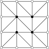
Figure 1: Local DMP does not imply a global DMP

numbered as in Sect. 2. Let $u_{1}=\dots=u_{4}=1$ (values at the black interior vertices) and $u_{5}=\dots=u_{16}=0$ (values at the white boundary vertices). Let the index sets $S_{i}$ be given by (34). Then the local DMP

$$u_{i}\leq\max_{j\in S_{i}}\,u_{j}\,,\qquad\quad i=1,\dots,4\,,$$

is satisfied but the corresponding global DMP (the right-hand sides of the implications (53) and (55) with $M=4$ and $N=16$) does not hold.

5 An error estimate

In the previous section, we analyzed the nonlinear algebraic problem (35), (36) on its own, without relating it to some discretization (except for Theorem 4). If the algebraic problem originates from a discretization of the convection–diffusion–reaction problem (1), then a natural question is how well its solution approximates the solution $u$ of (1). This question will be briefly addressed in this section.

Let us assume that the algebraic problem (16), (17) corresponds to the variational problem (9) satisfying (11), i.e., it is defined by (13)–(15). Let $u_{h}\in W_{h}$ correspond to the solution ${\rm U}\in{\mathbb{R}}^{N}$ of the nonlinear algebraic problem (35), (36) via (8). Our aim is to estimate the error $u-u_{h}$. To this end, it is of advantage to write the nonlinear algebraic problem in a variational form. We denote

$$b_{h}(w\mathchar 24635\relax\;z,v)=\sum_{i,j=1}^{N}\,b_{ij}(w)\,z(x_{j})\,v(x_{i})\qquad\forall\,\,w,z,v\in C(\overline{\Omega})\,,$$

with $b_{ij}(w):=b_{ij}(\{w(x_{i})\}_{i=1}^{N})$. Then the nonlinear algebraic problem (35), (36) is equivalent to the following variational problem:

Find $u_{h}\in W_{h}$ such that $u_{h}(x_{i})=u_{b}(x_{i})$, $i=M+1,\dots,N$, and

$$a_{h}(u_{h},v_{h})+b_{h}(u_{h}\mathchar 24635\relax\;u_{h},v_{h})=(g,v_{h})\qquad\forall\,\,v_{h}\in V_{h}\,.$$

In view of (29)–(31), for any $w\in C(\overline{\Omega})$, the mapping $b_{h}(w\mathchar 24635\relax\;\cdot,\cdot)$ is a nonnegative symmetric bilinear form on $C(\overline{\Omega})\times C(\overline{\Omega})$ and hence the functional $(b_{h}(w\mathchar 24635\relax\;\cdot,\cdot))^{1/2}$ is a seminorm on $C(\overline{\Omega})$. Thus, for estimating the error $u-u_{h}$, it is natural to use a solution-dependent norm on $V_{h}$ defined by

$$\|v_{h}\|_{h}:=\Big{(}C_{a}\,\|v_{h}\|_{a}^{2}+b_{h}(u_{h}\mathchar 24635\relax\;v_{h},v_{h})\Big{)}^{1/2}\,,\qquad v_{h}\in V_{h}\,,$$

where $C_{a}$ and $\|\cdot\|_{a}$ are the same as in (11). Note that $\|\cdot\|_{h}$ may be only a seminorm on $W_{h}$ and that it is not defined on the space $H^{1}(\Omega)$. Assuming that $u\in C(\overline{\Omega})$ and using the techniques of BJK16 , one obtains the estimate

$$\|u-u_{h}\|_{h}\leq C_{a}^{1/2}\,\|u-i_{h}u\|_{a}+\sup_{v_{h}\in V_{h}}\frac{a(u,v_{h})-a_{h}(i_{h}u,v_{h})}{\|v_{h}\|_{h}}$$

$$\hskip 170.71652pt+(b_{h}(u_{h}\mathchar 24635\relax\;i_{h}u,i_{h}u))^{1/2}\,,$$ (62)

where $i_{h}:C(\overline{\Omega})\to W_{h}$ is the usual Lagrange interpolation operator. The last term on the right-hand side represents an estimate of the consistency error originating from the algebraic stabilization.

In what follows, we shall assume that either $a_{h}=a$ or $a_{h}$ is defined by (10) so that one can use the norm $\|\cdot\|_{a}$ given by (12) and consider $C_{a}=1$. For simplicity, we shall assume that $\sigma_{0}>0$ and refer to BJK16 for the case $\sigma_{0}=0$. Assuming that $u\in H^{2}(\Omega)$, standard interpolation estimates (cf. Ciarlet ) give

$$\|u-i_{h}u\|_{a}\leq C\,(\varepsilon+\sigma_{0}\,h^{2})^{1/2}\,h\,|u|_{2,\Omega}\,.$$ (63)

Moreover, it was shown in BJK16 that one has

$$\sup_{v_{h}\in V_{h}}\frac{a(u,v_{h})-a_{h}(i_{h}u,v_{h})}{\|v_{h}\|_{h}}\leq C\,(\varepsilon+\sigma_{0}^{-1}\,\{\|{\boldsymbol{b}}\|_{0,\infty,\Omega}^{2}+\|c\|_{0,\infty,\Omega}^{2}\})^{1/2}\,h\,\|u\|_{2,\Omega}\,.$$ (64)

To estimate the last term in (62), we assume that (33) holds with $S_{i}$ defined in (34) for all $i=1,\dots,N$. Then it follows using (38) and (31) that

$$b_{h}(u_{h}\mathchar 24635\relax\;i_{h}u,i_{h}u) =-\frac{1}{2}\sum_{i=1}^{N}\,\sum_{j\in S_{i}}\,b_{ij}(u_{h})\,[u(x_{i})-u(x_{j})]^{2}$$

$$\leq\sum_{T\in{\mathscr{T}}_{h}}\,\sum_{x_{i},x_{j}\in T}\,|b_{ij}(u_{h})|\,[u(x_{i})-u(x_{j})]^{2}$$

$$\leq\sum_{T\in{\mathscr{T}}_{h}}\,\sum_{x_{i},x_{j}\in T}\,|b_{ij}(u_{h})|\,\|x_{i}-x_{j}\|^{2}\|(\nabla i_{h}u)|_{T}\|^{2}\,,$$

where $\|\cdot\|$ is the Euclidean norm on ${\mathbb{R}}^{d}$. Thus, using the shape regularity of ${\mathscr{T}}_{h}$ and denoting

$$A_{h}(u_{h})=\max_{i,j=1,\dots,N,\,i\neq j}\,\left(|b_{ij}(u_{h})|\,\|x_{i}-x_{j}\|^{2-d}\right),$$

one has

$$b_{h}(u_{h}\mathchar 24635\relax\;i_{h}u,i_{h}u)\leq C\,A_{h}(u_{h})\,|i_{h}u|_{1,\Omega}^{2}\,.$$

The behavior of $A_{h}(u_{h})$ with respect to $h$ depends on how the artificial diffusion matrix is constructed. Often (e.g., in the next two sections), one has

$$|b_{ij}(u_{h})|\leq\max\{|a_{ij}|,|a_{ji}|\}\qquad\forall\,\,i\neq j\,.$$ (65)

Then (cf. the proofs of (BJK16, , Lemma 16) and (BJK18, , Lemma 2))

$$|b_{ij}(u_{h})|\leq C\,(\varepsilon+\|{\boldsymbol{b}}\|_{0,\infty,\Omega}\,h+\|c\|_{0,\infty,\Omega}\,h^{2})\,\|x_{i}-x_{j}\|^{d-2}\qquad\forall\,\,i\neq j\,,$$

and hence

$$b_{h}(u_{h}\mathchar 24635\relax\;i_{h}u,i_{h}u)\leq C\,(\varepsilon+\|{\boldsymbol{b}}\|_{0,\infty,\Omega}\,h+\|c\|_{0,\infty,\Omega}\,h^{2})\,|i_{h}u|_{1,\Omega}^{2}\,.$$ (66)

Finally, substituting the estimates (63), (64), and (66) in (62), one obtains the estimate

$$\|u-u_{h}\|_{h} \leq C\,(\varepsilon+\sigma_{0}^{-1}\,\{\|{\boldsymbol{b}}\|_{0,\infty,\Omega}^{2}+\|c\|_{0,\infty,\Omega}^{2}\}+\sigma_{0}h^{2})^{1/2}\,h\,\|u\|_{2,\Omega}$$

$$\hskip 45.5244pt+C\,(\varepsilon+\|{\boldsymbol{b}}\|_{0,\infty,\Omega}\,h+\|c\|_{0,\infty,\Omega}\,h^{2})^{1/2}\,|i_{h}u|_{1,\Omega}\,.$$ (67)

Note that, in all the above estimates, the constant $C$ is independent of $h$ and the data of problem (1).

As one can see, the estimate (67) implies the convergence order $1/2$ in the convection-dominated case and no convergence in the diffusion-dominated case. It was demonstrated in BJK16 that this result is sharp under the above assumptions on the artificial diffusion matrix. However, for particular definitions of $b_{ij}$ and/or particular types of triangulations, a better convergence behavior can be observed numerically and in a few special cases also proved. We refer to BJK16 , BJK17 , and BJK18 for a refined analysis and various numerical results.

6 Algebraic flux correction

In this section we present an example of the nonlinear algebraic problem (35), (36) based on algebraic flux correction (AFC).

A detailed derivation of an AFC scheme for problem (16), (17) can be found, e.g., in BJK16 . The idea is to add the term $({\mathbb{D}}\,{\rm U})_{i}$ to both sides of (16) (so that, on the left-hand side, one has the same matrix as in the stabilized problem (26)) and then, on the right-hand side, to use the identity

$$({\mathbb{D}}\,{\rm U})_{i}=\sum_{j=1}^{N}\,f_{ij}\qquad\mbox{with}\qquad f_{ij}=d_{ij}\,(u_{j}-u_{i})$$

and to limit those anti-diffusive fluxes $f_{ij}$ that would otherwise cause spurious oscillations. The limiting is achieved by multiplying the fluxes by solution dependent limiters $\alpha_{ij}\in[0,1]$. This leads to the nonlinear algebraic problem

$$\sum_{j=1}^{N}\,a_{ij}\,u_{j}+\sum_{j=1}^{N}\,(1-\alpha_{ij}({\rm U}))\,d_{ij}\,(u_{j}-u_{i})=g_{i}\,,\qquad i=1,\dots,M\,,$$ (68)

$$u_{i}=u^{b}_{i}\,,\qquad i=M+1,\dots,N\,.$$ (69)

It is assumed that

$$\alpha_{ij}=\alpha_{ji}\,,\qquad i,j=1,\dots,N\,,$$ (70)

and that, for any $i,j\in\{1,\dots,N\}$, the function $\alpha_{ij}({\rm U})(u_{j}-u_{i})$ is a continuous function of ${\rm U}\in{\mathbb{R}}^{N}$. A theoretical analysis of the AFC scheme (68), (69) concerning the solvability, local DMP and error estimation can be found in BJK16 .

The symmetry condition (70) is particularly important for several reasons. First, it guarantees that the resulting method is conservative. Second, it implies that the matrix corresponding to the term arising from the AFC is positive semidefinite. This shows that this term really enhances the stability of the method and enables to estimate the error of the approximate solution, see BJK16 . Finally, it was demonstrated in BJK15 that, without the symmetry condition (70), the nonlinear algebraic problem (68), (69) is not solvable in general.

In view of the equivalence between (35) and (37), it is obvious that (68) can be written in the form (35) with

$$b_{ij}({\rm U})=(1-\alpha_{ij}({\rm U}))\,d_{ij}\qquad\forall\,\,i\neq j\,,\qquad\qquad b_{ii}({\rm U})=-\sum_{j\neq i}\,b_{ij}({\rm U})\,.$$ (71)

This matrix $(b_{ij}({\rm U}))_{i,j=1}^{N}$ satisfies the assumptions (29)–(31) and (33) with $S_{i}$ defined by (28).

Of course, the properties of the AFC scheme (68), (69) significantly depend on the choice of the limiters $\alpha_{ij}$. Here we present the Kuzmin limiter proposed in Kuzmin07 which was thoroughly investigated in BJK16 and can be considered as a standard limiter for algebraic stabilizations of steady-state convection–diffusion–reaction equations.

To define the limiter of Kuzmin07 , one first computes, for $i=1,\dots,M$,

$$P_{i}^{+}=\sum_{\mbox{\parbox{22.76219pt}{\scriptsize\centerline{\hbox{$j{=}1$}} \centerline{\hbox{$a_{ji}\leq a_{ij}$}}}}}^{N}\,f_{ij}^{+}\,,\quad\,\,\,P_{i}^{-}=\sum_{\mbox{\parbox{22.76219pt}{\scriptsize\centerline{\hbox{$j{=}1$}} \centerline{\hbox{$a_{ji}\leq a_{ij}$}}}}}^{N}\,f_{ij}^{-}\,,\quad\,\,\,Q_{i}^{+}=-\sum_{j=1}^{N}\,f_{ij}^{-}\,,\quad\,\,\,Q_{i}^{-}=-\sum_{j=1}^{N}\,f_{ij}^{+}\,,$$ (72)

where $f_{ij}=d_{ij}\,(u_{j}-u_{i})$, $f_{ij}^{+}=\max\{0,f_{ij}\}$, and $f_{ij}^{-}=\min\{0,f_{ij}\}$. Then, one defines

$$R_{i}^{+}=\min\left\{1,\frac{Q_{i}^{+}}{P_{i}^{+}}\right\},\quad R_{i}^{-}=\min\left\{1,\frac{Q_{i}^{-}}{P_{i}^{-}}\right\},\qquad i=1,\dots,M\,.$$ (73)

If $P_{i}^{+}$ or $P_{i}^{-}$ vanishes, one sets $R_{i}^{+}=1$ or $R_{i}^{-}=1$, respectively. For $i=M+1,\dots,N$, one defines $R_{i}^{+}=R_{i}^{-}=1$. Furthermore, one sets

$$\widetilde{\alpha}_{ij}=\left\{\begin{array}[]{cl}R_{i}^{+}&\mbox{if}\,\,\,f_{ij}>0\,,\\ 1&\mbox{if}\,\,\,f_{ij}=0\,,\\ R_{i}^{-}&\mbox{if}\,\,\,f_{ij}<0\,,\end{array}\right.\qquad\qquad i,j=1,\dots,N\,.$$ (74)

Finally, one defines

$$\alpha_{ij}=\alpha_{ji}=\widetilde{\alpha}_{ij}\qquad\mbox{if}\quad a_{ji}\leq a_{ij}\,,\qquad i,j=1,\dots,N\,.$$ (75)

It was proved in BJK16 that the AFC scheme (68), (69) with the above limiter satisfies the local DMP (21) with $S_{i}$ defined by (20) provided that

$$a_{ij}+a_{ji}\leq 0\qquad\forall\,\,i,j=1,\dots,N\,,\,\,i\neq j\,,\,\,i\leq M\,\,\mbox{or}\,\,j\leq M\,.$$ (76)

The local DMP (23) holds under the additional condition (24). In Kno17 , it was proved that the assumption (76) can be weakened to

$$\min\{a_{ij},a_{ji}\}\leq 0\qquad\forall\,\,i=1,\dots,M\,,\,\,j=1,\dots,N\,,\,\,i\neq j\,.$$ (77)

Then the local DMP (21) holds with $S_{i}$ defined by (28) and, if (24) is satisfied, then again also the local DMP (23) is valid.

If the AFC scheme (68), (69) is applied to the algebraic problem (16), (17) defined by (13)–(15) with $a_{h}$ given by (10), then, as discussed in BJK16 , the validity of (76) is guaranteed if the triangulation ${\mathscr{T}}_{h}$ is weakly acute, i.e., if the angles between facets of ${\mathscr{T}}_{h}$ do not exceed $\pi/2$. In the two-dimensional case, (76) holds if and (in principle) only if ${\mathscr{T}}_{h}$ is a Delaunay triangulation, i.e., the sum of any pair of angles opposite a common edge is smaller than, or equal to, $\pi$ (the note ‘in principle’ is added because angles opposite interior edges having both end points on the boundary of $\Omega$ can be arbitrary). The condition (77) may be satisfied also for non-Delaunay triangulations, particularly, in the convection-dominated case, since the convection matrix is skew-symmetric. However, in general, the validity of a DMP cannot be guaranteed for non-Delaunay triangulations. Moreover, if the lumped bilinear form (10) is replaced by the original bilinear form (3), then the validity of the conditions (76) or (77) may be lost since some off-diagonal entries of the matrix corresponding to the reaction term from (3) are positive.

It was shown in Kno17 that the DMP generally does not hold if condition (77) is not satisfied. This is due to the condition $a_{ji}\leq a_{ij}$ used in (75) to symmetrize the factors $\widetilde{\alpha}_{ij}$. It suffices to study this condition for $i\leq M$ or $j\leq M$ since $\alpha_{ij}$ with $i,j\in\{M+1,\dots,N\}$ does not occur in (68). Then, if the discretizations from Sect. 2 are considered, the symmetry of the bilinear forms corresponding to the diffusion and reaction terms implies that the condition $a_{ji}<a_{ij}$ is equivalent to the inequality

$$({{\boldsymbol{b}}}\cdot\nabla\varphi_{j},\varphi_{i})>0\,.$$

As it was discussed in Kno17 , in many cases (depending on ${\boldsymbol{b}}$ and the geometry of the triangulation), this inequality means that the vertex $x_{i}$ lies in the upwind direction with respect to the vertex $x_{j}$. Consequently, the use of the inequality $a_{ji}<a_{ij}$ in the definition of the above limiter causes that $\alpha_{ij}=\alpha_{ji}$ is defined using quantities computed at the upwind vertex of the edge with end points $x_{i}$, $x_{j}$. It turns out that this feature has a positive influence on the quality of the approximate solutions and on the convergence of the iterative process for solving the nonlinear problem (68), (69).

In order to obtain a method satisfying the DMP on arbitrary meshes and preserving the upwind feature described above, modifications of $\alpha_{ij}=\alpha_{ji}$ were considered in Kno17 ; Kno19 if $\min\{a_{ij},a_{ji}\}>0$. In the present paper, we shall achieve this goal by changing the definition of the matrix ${\mathbb{B}}({\rm U})$ in (71). First, however, we shall derive an equivalent form of the above limiter under the assumption (77). Note that, without this assumption, the application of the limiter does not make much sense since the main goal of the AFC, i.e., the validity of the DMP, is not achieved in general. Moreover, if (77) does not hold, the AFC scheme is not uniquely defined because the symmetrization (75) is ambiguous if $a_{ij}=a_{ji}$. If (77) holds, this ambiguity does not influence the resulting method since $d_{ij}=0$ for $a_{ij}=a_{ji}$ and hence the respective $\alpha_{ij}=\alpha_{ji}$ does not occur in the nonlinear problem (68), (69) and can be defined arbitrarily.

Thus, let us assume that (77) holds. Then, for any $i\in\{1,\dots,M\}$ and $j\in\{1,\dots,N\}$ with $i\neq j$, one has the equivalence

$$a_{ji}\leq a_{ij}\quad\mbox{and}\quad d_{ij}\neq 0\qquad\Leftrightarrow\qquad a_{ij}>0\,.$$

Moreover, if $a_{ij}>0$, then $d_{ij}=-a_{ij}$. Therefore, it follows from (72) that

$$P_{i}^{+}=\sum_{\mbox{\parbox{22.76219pt}{\scriptsize\centerline{\hbox{$j{=}1$}} \centerline{\hbox{$a_{ij}>0$}}}}}^{N}\,a_{ij}\,(u_{i}-u_{j})^{+}\,,\qquad\quad P_{i}^{-}=\sum_{\mbox{\parbox{22.76219pt}{\scriptsize\centerline{\hbox{$j{=}1$}} \centerline{\hbox{$a_{ij}>0$}}}}}^{N}\,a_{ij}\,(u_{i}-u_{j})^{-}\,.$$ (78)

Furthermore, we shall rewrite the formulas for $Q_{i}^{\pm}$ and $\widetilde{\alpha}_{ij}$. For this, the validity of (77) will not be needed. Since, for any real number $a$, its positive and negative parts satisfy $-a^{-}=(-a)^{+}$ and $-a^{+}=(-a)^{-}$, one has

$$Q_{i}^{+}=\sum_{j=1}^{N}\,|d_{ij}|\,(u_{j}-u_{i})^{+}\,,\qquad\quad Q_{i}^{-}=\sum_{j=1}^{N}\,|d_{ij}|\,(u_{j}-u_{i})^{-}\,.$$ (79)

If $d_{ij}\neq 0$, then

$$\widetilde{\alpha}_{ij}=\left\{\begin{array}[]{cl}R_{i}^{+}&\mbox{if}\,\,\,u_{i}>u_{j}\,,\\ 1&\mbox{if}\,\,\,u_{i}=u_{j}\,,\\ R_{i}^{-}&\mbox{if}\,\,\,u_{i}<u_{j}\,.\end{array}\right.\qquad\qquad$$ (80)

If $d_{ij}=0$, then (80) generally gives another value than (74) but since $\alpha_{ij}$ is multiplied by $d_{ij}$ in (68), the use of (80) does not change the AFC scheme. Thus, if the condition (77) is satisfied, then defining the limiter $\alpha_{ij}$ in the AFC scheme (68), (69) by (78), (79), (73), (80), and (75) is equivalent to using (72)–(75).

7 A new algebraically stabilized scheme

As discussed in the preceding section, the symmetrization (75) of the limiter causes that the DMP does not hold for the AFC scheme (68), (69) in general. In this section we modify the AFC scheme in such a way that the symmetry of the limiter will not be needed and the DMP will be always satisfied.

To make the formulas clearer, we denote

$$\beta_{ij}=1-\alpha_{ij}\,.$$ (81)

As we know, the AFC scheme (68), (69) can be written in the form (35), (36) with the artificial diffusion matrix ${\mathbb{B}}({\rm U})=(b_{ij}({\rm U}))_{i,j=1}^{N}$ given in (71). In view of (25) and (70), one observes that the off-diagonal entries of this matrix satisfy

$$b_{ij}({\rm U})=-\beta_{ij}({\rm U})\max\{a_{ij},0,a_{ji}\}=-\max\{\beta_{ij}({\rm U})\,a_{ij},0,\beta_{ji}({\rm U})\,a_{ji}\}\,.$$

This motivates us to define the artificial diffusion matrix by

$$b_{ij}({\rm U}) =-\max\{\beta_{ij}({\rm U})\,a_{ij},0,\beta_{ji}({\rm U})\,a_{ji}\}\,,\qquad i,j=1,\dots,N\,,\,\,i\neq j\,,$$ (82)

$$b_{ii}({\rm U}) =-\sum_{\mbox{\parbox{11.38109pt}{\scriptsize\centerline{\hbox{$j{=}1$}} \centerline{\hbox{$j{\neq}i$}}}}}^{N}\,b_{ij}({\rm U})\,,\qquad i=1,\dots,N\,.$$ (83)

Obviously, this matrix $(b_{ij}({\rm U}))_{i,j=1}^{N}$ again satisfies the assumptions (29)–(31) and (33) with $S_{i}$ defined by (28). Note however that, in contrast to (71), the formula (82) leads to a symmetric matrix ${\mathbb{B}}({\rm U})$ also if the limiters $\alpha_{ij}$ are not symmetric. This enables us to get rid of the symmetry condition (70).

Thus, we shall consider the algebraic problem (35), (36) with the artificial diffusion matrix given by (82) and (83) and with any functions $\beta_{ij}$ satisfying, for any $i,j\in\{1,\dots,N\}$,

$$\beta_{ij}\,:\,{\mathbb{R}}^{N}\to[0,1]\,,$$ (84)

$$\mbox{if $a_{ij}>0$, then $\beta_{ij}({\rm U})(u_{j}-u_{i})$ is a continuous function of ${\rm U}\in{\mathbb{R}}^{N}$}\,.$$ (85)

No other assumptions on $\beta_{ij}$ will be made in the general case.

First let us state an existence result.

Theorem 5.

Let (19) hold and let the matrix $(b_{ij}({\rm U}))_{i,j=1}^{N}$ be defined by (82) and (83) with functions $\beta_{ij}$ satisfying (84) and (85) for any $i,j\in\{1,\dots,N\}$. Then Assumption (A1) is satisfied and the nonlinear algebraic problem (35), (36) has a solution.

Proof: In view of Theorem 1, it suffices to verify the validity of Assumption (A1). Consider any $i,j\in\{1,\dots,N\}$ with $i\neq j$. Due to (84), it is obvious that $b_{ij}({\rm U})$ is bounded on ${\mathbb{R}}^{N}$ and it remains to show the continuity of $\Phi({\rm U}):=b_{ij}({\rm U})(u_{j}-u_{i})$. Due to the definition of $b_{ij}({\rm U})$, this is particularly easy if $a_{ij}\leq 0$ or $a_{ji}\leq 0$ since $\Phi({\rm U})\equiv 0$ if both $a_{ij}$ and $a_{ji}$ are nonpositive and otherwise the continuity of $\Phi({\rm U})$ immediately follows from (85). Thus, let $a_{ij}>0$ and $a_{ji}>0$. Choose any $\bar{\rm U}=(\bar{u}_{1},\dots,\bar{u}_{N})\in\mathbb{R}^{N}$ and let us show that $\Phi$ is continuous at the point $\bar{\rm U}$. If $\bar{u}_{i}=\bar{u}_{j}$, then $\Phi(\bar{\rm U})=0$ and the continuity at $\bar{\rm U}$ follows from the estimates

$$|\Phi({\rm U})-\Phi(\bar{\rm U})|=|\Phi({\rm U})|\leq C\,|u_{i}-u_{j}|\leq C\,\sqrt{2}\,\|{\rm U}-\bar{\rm U}\|\,,$$ (86)

where $\|\cdot\|$ is the Euclidean norm on ${\mathbb{R}}^{N}$. Thus, let $\bar{u}_{i}\neq\bar{u}_{j}$. Without loss of generality, one can assume that $\bar{u}_{i}>\bar{u}_{j}$. Then, if ${\rm U}\in{\mathbb{R}}^{N}$ satisfies $\|{\rm U}-\bar{\rm U}\|\leq\frac{1}{2}|\bar{u}_{i}-\bar{u}_{j}|$, one has $u_{i}>u_{j}$ and hence

$$\Phi({\rm U})=\max\{\beta_{ij}({\rm U})\,(u_{i}-u_{j})\,a_{ij},\beta_{ji}({\rm U})\,(u_{i}-u_{j})\,a_{ji}\}\,.$$

Since the maximum of two continuous functions is continuous, it follows from (85) that $\Phi$ is continuous in a neighborhood of $\bar{\rm U}$, which completes the proof.

If the functions $\beta_{ij}$ form a symmetric matrix and $\alpha_{ij}$ satisfy (81), then the matrix ${\mathbb{B}}({\rm U})$ defined by (82), (83) satisfies (71) and method (35), (36) can be written in the form (68), (69). Hence, in this case, the AFC scheme is recovered.

Another interesting observation can be made if condition (77) is satisfied. Consider any $i\in\{1,\dots,M\}$ and $j\in\{1,\dots,N\}$ with $i\neq j$. Then, if $a_{ij}>0$, one has $a_{ji}\leq 0$ and hence $b_{ij}({\rm U})=-\beta_{ij}({\rm U})\,a_{ij}=\beta_{ij}({\rm U})\,d_{ij}$. Similarly, if $a_{ji}>0$, then $a_{ij}\leq 0$ and hence $b_{ij}({\rm U})=-\beta_{ji}({\rm U})\,a_{ji}=\beta_{ji}({\rm U})\,d_{ij}$. If both $a_{ij}\leq 0$ and $a_{ji}\leq 0$, then $b_{ij}({\rm U})=0$ and $d_{ij}=0$. Thus, one concludes that

$$b_{ij}({\rm U})=\left\{\begin{array}[]{cl}\beta_{ij}({\rm U})\,d_{ij}&\mbox{if}\,\,\,a_{ji}\leq a_{ij}\,,\\ \beta_{ji}({\rm U})\,d_{ij}&\mbox{otherwise}\,,\end{array}\right.$$

for $i=1,\dots,M$ and $j=1,\dots,N$ with $i\neq j$. Thus, if (77) holds, then the definition (82) implicitly comprises the favorable upwind feature discussed in the preceding section and the method (35), (36) can be again written in the form of the AFC scheme (68), (69). Moreover, if one sets

$$\beta_{ij}=1-\widetilde{\alpha}_{ij}\,,$$ (87)

then one obtains the AFC scheme (68), (69) with limiters $\alpha_{ij}$ defined by (75). Consequently, if the condition (77) holds, then the AFC scheme (68), (69) with limiters $\alpha_{ij}$ defined by (72)–(75) is equivalent to the system (35), (36) with ${\mathbb{B}}({\rm U})$ defined by (82), (83), and (87) with $\widetilde{\alpha}_{ij}$ given by (78), (79), (73), and (80). Therefore, this new method preserves the advantages of the AFC scheme from the preceding section which are available under condition (77). However, in contrast to the method from the preceding section, we shall see that the new method satisfies the DMP also if condition (77) is not satisfied.

For the convenience of the reader, we first summarize the definition of $\beta_{ij}$ in the new method. We shall make a slight change in (79) and replace $|d_{ij}|=\max\{a_{ij},0,a_{ji}\}$ by

$$q_{ij}=\max\{|a_{ij}|,a_{ji}\}\,,$$ (88)

which is larger or equal to $|d_{ij}|$. This heuristic modification may improve the accuracy and convergence behavior in the diffusion-dominated case when the method is applied to the discretizations from Sect. 2 and non-Delaunay meshes are used, see the discussion in Sect. 8. One could also consider the symmetric variant $\max\{|a_{ij}|,|a_{ji}|\}$ which often leads to very similar results as (88), however, in a few cases, we observed that (88) is more convenient from the point of view of both the quality of the solution and the convergence of the solver used to solve the nonlinear discrete problem. Thus, the final definition of $\beta_{ij}$ is as follows. For any $i\in\{1,\dots,M\}$, set

$$P_{i}^{+}=\sum_{\mbox{\parbox{22.76219pt}{\scriptsize\centerline{\hbox{$j{=}1$}} \centerline{\hbox{$a_{ij}>0$}}}}}^{N}\,a_{ij}\,(u_{i}-u_{j})^{+}\,,\qquad\quad P_{i}^{-}=\sum_{\mbox{\parbox{22.76219pt}{\scriptsize\centerline{\hbox{$j{=}1$}} \centerline{\hbox{$a_{ij}>0$}}}}}^{N}\,a_{ij}\,(u_{i}-u_{j})^{-}\,,$$ (89)

$$Q_{i}^{+}=\sum_{j=1}^{N}\,q_{ij}\,(u_{j}-u_{i})^{+}\,,\qquad\quad Q_{i}^{-}=\sum_{j=1}^{N}\,q_{ij}\,(u_{j}-u_{i})^{-}\,,$$ (90)

$$R_{i}^{+}=\min\left\{1,\frac{Q_{i}^{+}}{P_{i}^{+}}\right\}\,, R_{i}^{-}=\min\left\{1,\frac{Q_{i}^{-}}{P_{i}^{-}}\right\}\,,$$ (91)

where $q_{ij}$ is defined by (88). Furthermore, set

$$R_{i}^{+}=1\,,\qquad R_{i}^{-}=1\,,\qquad\quad i=M+1,\dots,N\,.$$ (92)

Then define

$$\beta_{ij}=\left\{\begin{array}[]{ll}1-R_{i}^{+}&\mbox{if}\,\,\,u_{i}>u_{j}\,,\\ 0&\mbox{if}\,\,\,u_{i}=u_{j}\,,\\ 1-R_{i}^{-}&\mbox{if}\,\,\,u_{i}<u_{j}\,,\end{array}\right.\qquad\qquad i,j=1,\dots,N\,.$$ (93)

Remark 6.

If $P_{i}^{+}=0$, then $R_{i}^{+}$ can be defined arbitrarily (and the same holds for $P_{i}^{-}$ and $R_{i}^{-}$). Indeed, $P_{i}^{+}$ is used only for defining $\beta_{ij}$ with $j$ such that $u_{i}>u_{j}$. Then, if $P_{i}^{+}=0$, one has $a_{ij}\leq 0$ and hence the matrix ${\mathbb{B}}({\rm U})$ defined by (82), (83) does not depend on these $\beta_{ij}$.

In view of Theorem 5, the following lemma implies that the problem (35), (36) with the artificial diffusion matrix defined by (82), (83) and (89)–(93) is solvable.

Lemma 1.

The functions $\beta_{ij}$ defined by (89)–(93) satisfy the assumption (85) for all $i,j\in\{1,\dots,N\}$.

Proof: Consider any $i,j\in\{1,\dots,N\}$ such that $i\neq j$ and $a_{ij}>0$ and any $\bar{\rm U}=(\bar{u}_{1},\dots,\bar{u}_{N})\in\mathbb{R}^{N}$. Like in the proof of Theorem 5, we want to show that $\Phi({\rm U}):=\beta_{ij}({\rm U})(u_{j}-u_{i})$ is continuous at the point $\bar{\rm U}$. If $\bar{u}_{i}=\bar{u}_{j}$, the continuity follows again from (86). If $\bar{u}_{i}>\bar{u}_{j}$, one again uses the fact that $u_{i}>u_{j}$ for ${\rm U}$ in a ball $B$ around $\bar{\rm U}$. Thus, for ${\rm U}\in B$, one has

$$\Phi({\rm U})=(1-R^{+}_{i}({\rm U}))\,(u_{j}-u_{i}).$$

Since both $P_{i}^{+}$ and $Q_{i}^{+}$ are continuous and $P_{i}^{+}$ is positive in $B$, the function $\Phi$ is continuous in $B$ and hence also at $\bar{\rm U}$. If $\bar{u}_{i}<\bar{u}_{j}$, one proceeds analogously.

Remark 7.

It is easy to show that $\beta_{ij}({\rm U})=\beta_{ij}(\alpha\,{\rm U})$ for any ${\rm U}\in{\mathbb{R}}^{N}$ and any $\alpha\neq 0$. This implies that $\beta_{ij}$ itself is not continuous since otherwise one would conclude that $\beta_{ij}({\rm U})=0$ for any ${\rm U}\in{\mathbb{R}}^{N}$ due to the fact that $\beta_{ij}(0)=0$.

Now let us investigate the validity of Assumption (A2).

Theorem 6.

Let the matrix $(b_{ij}({\rm U}))_{i,j=1}^{N}$ be defined by (82), (83) and (89)–(93). Then Assumption (A2) holds with $S_{i}$ defined in (28).

Proof: Consider any ${\rm U}=(u_{1},\dots,u_{N})\in\mathbb{R}^{N}$, $i\in\{1,\dots,M\}$, and $j\in S_{i}$. Let $u_{i}$ be a strict local extremum of $\rm U$ with respect to $S_{i}$. We want to prove that

$$a_{ij}+b_{ij}({\rm U})\leq 0\,.$$ (94)

If $a_{ij}\leq 0$, then (94) holds since $b_{ij}({\rm U})\leq 0$. Thus, let $a_{ij}>0$. If $u_{i}>u_{k}$ for any $k\in S_{i}$, then $P_{i}^{+}\geq a_{ij}\,(u_{i}-u_{j})^{+}>0$, $Q_{i}^{+}=0$ and hence $\beta_{ij}=1-R_{i}^{+}=1$. Similarly, if $u_{i}<u_{k}$ for any $k\in S_{i}$, then $P_{i}^{-}\leq a_{ij}\,(u_{i}-u_{j})^{-}<0$, $Q_{i}^{-}=0$ and hence $\beta_{ij}=1-R_{i}^{-}=1$. Thus, $b_{ij}({\rm U})\leq-a_{ij}$, which proves (94).

Theorems 5 and 6 show that, assuming the validity of (18) and (19), solutions of the nonlinear algebraic problem (35), (36) with the artificial diffusion matrix defined by (82), (83) and (89)–(93) satisfy all the versions of the DMP formulated in Theorems 2 and 3 and Corollary 1, without any additional assumptions on the matrix $\mathbb{A}$. Therefore, if this new method is applied to the algebraic problem (16), (17) defined by (13)–(15), the DMPs hold for both definitions (3) and (10) of the bilinear form and for any triangulation ${\mathscr{T}}_{h}$. Moreover, since $b_{ij}$ defined by (82) satisfies (65), the finite element function $u_{h}$ corresponding to the solution of (35), (36) satisfies the error estimate (67).

Remark 8.

If (89) is replaced by the original definition of $P_{i}^{\pm}$ from (72), then the algebraically stabilized scheme introduced in this section is not well defined. Indeed, in this case, $P_{i}^{\pm}$ may vanish also if $a_{ij}>0$ so that the corresponding $\beta_{ij}$ (which may be not well defined) is needed for computing the matrix ${\mathbb{B}}({\rm U})$ defined by (82), (83) (cf. also Remark 6). Moreover, one can show that, independently of how $R_{i}^{\pm}$ are defined in these cases, the continuity assumption (85) is not satisfied in general.

Remark 9.

As we already mentioned, a special case of the nonlinear algebraic problem (35), (36) with the artificial diffusion matrix defined by (82) and (83) is the AFC scheme from Sect. 6. Another example of a method having this structure is the nonlinear stabilization based on a graph-theoretic approach described in BB17 . Here, the artificial diffusion matrix ${\mathbb{B}}({\rm U})$ is given by

$$({\mathbb{B}}({\rm U})\,{\rm V})_{i}=\sum_{j\in S_{i}\cup\{i\}}\,\nu_{ij}({\rm U})\,l_{ij}\,v_{j}\qquad\forall\,\,{\rm V}\in{\mathbb{R}}^{N},\,i=1,\dots,N\,,$$

where $S_{i}$ is defined by (34), $l_{ij}:=2\,\delta_{ij}-1$ is the graph-theoretic Laplacian, and $\nu_{ij}$ is the artificial diffusion given by

$$\nu_{ij}({\rm U})=\max\{\alpha_{i}({\rm U})\,a_{ij},0,\alpha_{j}({\rm U})\,a_{ji}\}\quad\forall\,\,i\neq j\,,\qquad\nu_{ii}({\rm U})=\sum_{j\in S_{i}}\,\nu_{ij}({\rm U})\,,\qquad$$

with a shock detector $\alpha_{i}({\rm U})\in[0,1]$. Thus, the artificial diffusion matrix satisfies (82) and (83) with $\beta_{ij}=\alpha_{i}$ for $i,j=1,\dots,N$.

8 Numerical results

In the remaining part of the paper we shall refer to the system (35), (36) with the artificial diffusion matrix defined by (82), (83) and (89)–(93) as to the Monotone Upwind-type Algebraically Stabilized (MUAS) method. The AFC scheme with the Kuzmin limiter formulated in Sect. 6 will be simply called AFC scheme in the following. Our aim will now be to compare the AFC scheme with the MUAS method numerically for the finite element discretizations of (1) presented in Sect. 2. If not stated otherwise, the bilinear form (3) will be considered in the discrete problem.

Under condition (77), the only difference between the MUAS method and the AFC scheme consists in the definition of $Q_{i}^{\pm}$, cf. (90) and (79). Our numerical experiments show that the difference between the results of the two methods is very small in this case. Since numerical results for the AFC scheme under condition (77) have been reported in many other papers, we shall concentrate on cases where condition (77) is not satisfied.

As discussed in Sect. 6, condition (77) may be violated if the triangulation ${\mathscr{T}}_{h}$ is not of Delaunay type or if the reaction coefficient $c$ is sufficiently large in comparison with $\varepsilon$ and $\|{\boldsymbol{b}}\|$. We shall start with a reaction-dominated problem formulated in the following example.

Example 1.

(Reaction-dominated problem) Problem (1) is considered with $\Omega=(0,1)^{2}$, $\varepsilon=10^{-8}$, ${\boldsymbol{b}}=(0.004,0.012)^{T}$, $c=g=1$, and $u_{b}=0$.

A natural question is why not to set simply ${\boldsymbol{b}}=\mathbb{0}$ in Example 1. However, this would lead to a symmetric matrix $(a_{ij})_{i,j=1}^{N}$ and since the AFC scheme is not uniquely defined if $a_{ij}=a_{ji}>0$ for some indices $i\neq j$, it would be difficult to interpret the results. Note also that since $c$ and $g$ are constant in Example 1, equation (1) can be reformulated into a form with vanishing right-hand side. Indeed, if $u$ solves (1), then $(u-1)$ solves (1) with $g$ replaced by $0$ and $u_{b}=-1$. Then the maximum principles (4), (5) with $G=\Omega$ imply that $(u-1)\in[-1,0]$ and hence $u\in[0,1]$ in $\Omega$. The solution of (1) satisfies $u\approx 1$ away from layers which are located around the boundary of $\Omega$.

We will present results obtained on a uniform triangulation of the type depicted on the left of Fig. 2 containing $21\times 21$ vertices.

               

Figure 2: Types of triangulations considered in numerical experiments

Then the matrix $(a_{ij})_{i,j=1}^{N}$ defined by (13) with $a_{h}=a$ has only nonnegative entries and condition (77) is not satisfied. The AFC scheme does not satisfy the DMP and provides a nonphysical solution, see Fig. 3 (left).

Figure 3: Approximate solutions of Example 1 computed on a triangulation of the type shown on the left of Fig. 2: AFC method (left), AFC method with lumping (middle), MUAS method (right)

As discussed in Sect. 6, a possible remedy is to define the bilinear form $a_{h}$ by (10), i.e., to consider a lumping of the reaction term. This provides a physically consistent approximate solution but may lead to a smearing of the layers, see Fig. 3 (middle). On the other hand, applying the MUAS method, one obtains a very accurate solution with sharp layers, see Fig. 3 (right).

Example 2.

(Convection-dominated problem) Problem (1) is considered with $\Omega=(0,1)^{2}$, $\varepsilon=10^{-2}$, ${\boldsymbol{b}}=(\cos(-\pi/3),\sin(-\pi/3))^{T}$, $c=g=0$, and

$$u_{b}(x,y)=\left\{\begin{array}[]{ll}0&\quad\mbox{for $x=1$ or $y=0$,}\\ 1&\quad\mbox{else.}\end{array}\right.$$

To satisfy the assumptions on problem (1), the discontinuous function $u_{b}$ can be replaced by a smooth function such that the approximate solutions do not change for the triangulation considered in the numerical experiments.

This example will be used to demonstrate that the AFC scheme can lead to physically inconsistent solutions also in the convection-dominated case. To this end, one has to use a triangulation which is not of Delaunay type. We again consider a triangulation containing $21\times 21$ vertices which is now obtained from a triangulation of the type depicted on the right in Fig. 2 by shifting interior nodes to the right by half of the horizontal mesh width on each even horizontal mesh line. This gives a triangulation of the type shown in the middle of Fig. 2 for which condition (77) is again not satisfied. Like in Fig. 3, the results will be visualized using a uniform square mesh having the same number of vertices (and hence also the same horizontal mesh lines) as the mentioned triangulation.

According to the maximum principles (6), (7), the solution of (1) with the data specified in Example 2 satisfies $u\in[0,1]$ in $\Omega$. Fig. 4 (left) shows that this property is not preserved by the AFC scheme

       

Figure 4: Approximate solutions of Example 2 computed on a triangulation of the type shown in the middle of Fig. 2: AFC method (left), MUAS method (right)

for which the approximate solution contains a significant overshoot along the line $y=0$. On the other hand, the MUAS method provides a qualitatively correct approximate solution respecting the DMP, see Fig. 4 (right).

Example 3.

(Diffusion-dominated problem) Problem (1) is considered with $\Omega=(0,1)^{2}$, $\varepsilon=10$, ${\boldsymbol{b}}=(3,2)^{T}$, $c=1$, $u_{b}=0$, and the right-hand side $g$ chosen so that

$$u(x,y)=100\,x^{2}\,(1-x)^{2}\,y\,(1-y)\,(1-2y)$$

is the solution of (1).

In BJK16 , this example was considered on triangulations constructed similarly as the one in the middle of Fig. 2; the difference was that the shift of the respective interior nodes was only the tenth of the horizontal mesh width. It was observed that the convergence orders of the AFC scheme with respect to various norms tend to zero if fine meshes are used. This behavior is even more pronounced on meshes of the type shown in the middle of Fig. 2 (where the shift of the nodes is the half of the horizontal mesh width), see Table 1. In the tables, the value of $ne$ represents the number of edges along one horizontal mesh line (thus, $ne=6$ for the meshes in Fig. 2). Note that a lumping of the reaction term has no significant influence on the results in this case. On the other hand, applying the MUAS method, one observes a convergence in all the norms, see Table 2. This behavior is connected with the fact that the definition of $Q_{i}^{\pm}$ was changed from (79) to (90). If the original definition (79) is used in the MUAS method, then the accuracy deteriorates and the convergence orders tend to zero on fine meshes, see Table 3. Nevertheless, the convergence may fail also for the MUAS method when too distorted meshes are considered. An example is given in Table 4, where the results were computed on triangulations obtained from those of the type depicted on the right in Fig. 2 by shifting the respective interior nodes by eight tenths of the horizontal mesh width. However, also in this case the results are more accurate than in case of the AFC scheme.

A possible explanation of the observed deteriorations of convergence orders is the loss of the linearity preservation when using certain non-Delaunay meshes. Let us recall that the scheme (35) is called linearity preserving if ${\mathbb{B}}({\rm U})$ vanishes for any vector ${\rm U}$ representing a linear function in $\Omega$. Under further assumptions, this property enables to prove improved error estimates, see, e.g., BJK18 . It can be verified, that, in case of Table 2, the MUAS method is linearity preserving, which is not true for the schemes used to compute the results in Tables 1, 3, and 4. This could also explain why the replacement of (90) by (79) leads to the deterioration of the results since the absolute values of $Q_{i}^{\pm}$ given by (79) are smaller or equal to those given by (90) and hence the linearity preservation is more likely to hold if (90) is used.

Table 1: Errors and convergence orders of approximate solutions of Example 3 computed using the AFC scheme on triangulations of the type shown in the middle of Fig. 2

$ne$	$\|u-u_{h}\|_{0,\Omega}$	order	$|u-u_{h}|_{1,\Omega}$	order	$\|u-u_{h}\|_{h}$	order
16	5.636e$-$2	0.22	6.741e$-$1	0.41	2.626e$+$0	0.24
32	5.384e$-$2	0.07	5.908e$-$1	0.19	2.437e$+$0	0.11
64	5.332e$-$2	0.01	5.661e$-$1	0.06	2.380e$+$0	0.03
128	5.321e$-$2	0.00	5.593e$-$1	0.02	2.363e$+$0	0.01
256	5.319e$-$2	0.00	5.575e$-$1	0.00	2.358e$+$0	0.00
512	5.320e$-$2	0.00	5.570e$-$1	0.00	2.356e$+$0	0.00
1024	5.321e$-$2	0.00	5.568e$-$1	0.00	2.356e$+$0	0.00

Table 2: Errors and convergence orders of approximate solutions of Example 3 computed using the MUAS method on triangulations of the type shown in the middle of Fig. 2

$ne$	$\|u-u_{h}\|_{0,\Omega}$	order	$|u-u_{h}|_{1,\Omega}$	order	$\|u-u_{h}\|_{h}$	order
16	2.206e$-$2	1.60	4.847e$-$1	0.86	1.581e$+$0	0.88
32	6.967e$-$3	1.66	2.505e$-$1	0.95	8.038e$-$1	0.98
64	2.249e$-$3	1.63	1.263e$-$1	0.99	4.034e$-$1	0.99
128	7.770e$-$4	1.53	6.287e$-$2	1.01	2.003e$-$1	1.01
256	2.471e$-$4	1.65	3.115e$-$2	1.01	9.904e$-$2	1.02
512	7.108e$-$5	1.80	1.544e$-$2	1.01	4.901e$-$2	1.02
1024	1.915e$-$5	1.89	7.677e$-$3	1.01	2.433e$-$2	1.01

Table 3: Errors and convergence orders of approximate solutions of Example 3 computed using the MUAS method with $Q_{i}^{\pm}$ defined by (79) instead of (90). The used triangulations are of the type shown in the middle of Fig. 2

$ne$	$\|u-u_{h}\|_{0,\Omega}$	order	$|u-u_{h}|_{1,\Omega}$	order	$\|u-u_{h}\|_{h}$	order
16	7.677e$-$2	0.42	7.526e$-$1	0.40	3.019e$+$0	0.28
32	6.399e$-$2	0.26	6.382e$-$1	0.24	2.657e$+$0	0.18
64	5.806e$-$2	0.14	5.903e$-$1	0.11	2.488e$+$0	0.09
128	5.543e$-$2	0.07	5.711e$-$1	0.05	2.415e$+$0	0.04
256	5.426e$-$2	0.03	5.632e$-$1	0.02	2.383e$+$0	0.02
512	5.372e$-$2	0.01	5.598e$-$1	0.01	2.369e$+$0	0.01
1024	5.346e$-$2	0.01	5.582e$-$1	0.00	2.362e$+$0	0.00

Table 4: Errors and convergence orders of approximate solutions of Example 3 computed using the MUAS method on triangulations of the type depicted in the middle of Fig. 2 obtained by shifting the respective interior nodes by eight tenths of the horizontal mesh width

$ne$	$\|u-u_{h}\|_{0,\Omega}$	order	$|u-u_{h}|_{1,\Omega}$	order	$\|u-u_{h}\|_{h}$	order
16	4.589e$-$2	1.08	6.405e$-$1	0.70	2.303e$+$0	0.72
32	2.528e$-$2	0.86	3.834e$-$1	0.74	1.326e$+$0	0.80
64	1.714e$-$2	0.56	2.442e$-$1	0.65	8.316e$-$1	0.67
128	1.347e$-$2	0.35	1.758e$-$1	0.47	5.948e$-$1	0.48
256	1.178e$-$2	0.19	1.468e$-$1	0.26	4.956e$-$1	0.26
512	1.100e$-$2	0.10	1.355e$-$1	0.12	4.576e$-$1	0.12
1024	1.062e$-$2	0.05	1.311e$-$1	0.05	4.428e$-$1	0.05

Remark 10.

Comprehensive numerical studies of the MUAS method and, in particular, comparisons with the AFC schemes with Kuzmin limiter and with BJK limiter can be found in JJK21 . In this paper, the behavior of these methods on adaptively refined meshes, with conforming closure or with hanging vertices, is studied. The assessment focuses on the satisfaction of the global DMP, the accuracy of the numerical solutions, and the efficiency of the solver for the arising nonlinear problems.

References

- \bibcommenthead
- (1) Augustin, M., Caiazzo, A., Fiebach, A., Fuhrmann, J., John, V., Linke, A., Umla, R.: An assessment of discretizations for convection-dominated convection–diffusion equations. Comput. Methods Appl. Mech. Engrg. 200(47-48), 3395–3409 (2011)
- (2) Baba, K., Tabata, M.: On a conservative upwind finite element scheme for convective diffusion equations. RAIRO Anal. Numér. 15(1), 3–25 (1981)
- (3) Badia, S., Bonilla, J.: Monotonicity-preserving finite element schemes based on differentiable nonlinear stabilization. Comput. Methods Appl. Mech. Engrg. 313, 133–158 (2017)
- (4) Barrenechea, G.R., Burman, E., Karakatsani, F.: Blending low-order stabilised finite element methods: A positivity-preserving local projection method for the convection–diffusion equation. Comput. Methods Appl. Mech. Engrg. 317, 1169–1193 (2017)
- (5) Barrenechea, G.R., Burman, E., Karakatsani, F.: Edge-based nonlinear diffusion for finite element approximations of convection–diffusion equations and its relation to algebraic flux-correction schemes. Numer. Math. 135(2), 521–545 (2017)
- (6) Barrenechea, G.R., John, V., Knobloch, P.: Some analytical results for an algebraic flux correction scheme for a steady convection–diffusion equation in one dimension. IMA J. Numer. Anal. 35(4), 1729–1756 (2015)
- (7) Barrenechea, G.R., John, V., Knobloch, P.: Analysis of algebraic flux correction schemes. SIAM J. Numer. Anal. 54(4), 2427–2451 (2016)
- (8) Barrenechea, G.R., John, V., Knobloch, P.: An algebraic flux correction scheme satisfying the discrete maximum principle and linearity preservation on general meshes. Math. Models Methods Appl. Sci. 27(3), 525–548 (2017)
- (9) Barrenechea, G.R., John, V., Knobloch, P., Rankin, R.: A unified analysis of algebraic flux correction schemes for convection–diffusion equations. SeMA J. 75(4), 655–685 (2018)
- (10) Boris, J.P., Book, D.L.: Flux-corrected transport. I. SHASTA, a fluid transport algorithm that works. J. Comput. Phys. 11(1), 38–69 (1973)
- (11) Burman, E., Ern, A.: Nonlinear diffusion and discrete maximum principle for stabilized Galerkin approximations of the convection–diffusion-reaction equation. Comput. Methods Appl. Mech. Engrg. 191(35), 3833–3855 (2002)
- (12) Burman, E., Ern, A.: Stabilized Galerkin approximation of convection–diffusion–reaction equations: discrete maximum principle and convergence. Math. Comp. 74(252), 1637–1652 (2005)
- (13) Burman, E., Hansbo, P.: Edge stabilization for Galerkin approximations of convection–diffusion–reaction problems. Comput. Methods Appl. Mech. Engrg. 193(15-16), 1437–1453 (2004)
- (14) Ciarlet, P.G.: The Finite Element Method for Elliptic Problems. North-Holland, Amsterdam (1978)
- (15) Evans, L.C.: Partial Differential Equations, 2nd edn. American Mathematical Society, Providence, RI (2010)
- (16) Gilbarg, D., Trudinger, N.S.: Elliptic Partial Differential Equations of Second Order. Springer, Berlin (2001)
- (17) Guermond, J.-L., Nazarov, M., Popov, B., Yang, Y.: A second-order maximum principle preserving Lagrange finite element technique for nonlinear scalar conservation equations. SIAM J. Numer. Anal. 52(4), 2163–2182 (2014)
- (18) Gurris, M., Kuzmin, D., Turek, S.: Implicit finite element schemes for the stationary compressible Euler equations. Internat. J. Numer. Methods Fluids 69(1), 1–28 (2012)
- (19) Jha, A., John, V.: A study of solvers for nonlinear AFC discretizations of convection–diffusion equations. Comput. Math. Appl. 78(9), 3117–3138 (2019)
- (20) Jha, A., John, V., Knobloch, P.: Adaptive grids in the context of algebraic stabilizations for convection–diffusion–reaction equations. In preparation (2021)
- (21) John, V., Knobloch, P.: On spurious oscillations at layers diminishing (SOLD) methods for convection–diffusion equations: Part II – Analysis for and finite elements. Comput. Methods Appl. Mech. Engrg. 197(21-24), 1997–2014 (2008)
- (22) John, V., Schmeyer, E.: Finite element methods for time-dependent convection–diffusion–reaction equations with small diffusion. Comput. Methods Appl. Mech. Engrg. 198(3-4), 475–494 (2008)
- (23) Knobloch, P.: Improvements of the Mizukami–Hughes method for convection–diffusion equations. Comput. Methods Appl. Mech. Engrg. 196(1-3), 579–594 (2006)
- (24) Knobloch, P.: Numerical solution of convection–diffusion equations using a nonlinear method of upwind type. J. Sci. Comput. 43(3), 454–470 (2010)
- (25) Knobloch, P.: On the discrete maximum principle for algebraic flux correction schemes with limiters of upwind type. In: Huang, Z., Stynes, M., Zhang, Z. (eds.) Boundary and Interior Layers, Computational and Asymptotic Methods BAIL 2016. Lect. Notes Comput. Sci. Eng., vol. 120, pp. 129–139. Springer, Cham (2017)
- (26) Knobloch, P.: A linearity preserving algebraic flux correction scheme of upwind type satisfying the discrete maximum principle on arbitrary meshes. In: Radu, F.A., Kumar, K., Berre, I., Nordbotten, J.M., Pop, I.S. (eds.) Numerical Mathematics and Advanced Applications ENUMATH 2017. Lect. Notes Comput. Sci. Eng., vol. 126, pp. 909–918. Springer, Cham (2019)
- (27) Knobloch, P.: A new algebraically stabilized method for convection–diffusion–reaction equations. In: Vermolen, F.J., Vuik, C. (eds.) Numerical Mathematics and Advanced Applications ENUMATH 2019. Lect. Notes Comput. Sci. Eng., vol. 139, pp. 605–613. Springer, Cham (2021)
- (28) Kuzmin, D.: On the design of general-purpose flux limiters for finite element schemes. I. Scalar convection. J. Comput. Phys. 219(2), 513–531 (2006)
- (29) Kuzmin, D.: Algebraic flux correction for finite element discretizations of coupled systems. In: Papadrakakis, M., Oñate, E., Schrefler, B. (eds.) Proceedings of the Int. Conf. on Computational Methods for Coupled Problems in Science and Engineering, pp. 1–5. CIMNE, Barcelona (2007)
- (30) Kuzmin, D.: Explicit and implicit FEM-FCT algorithms with flux linearization. J. Comput. Phys. 228(7), 2517–2534 (2009)
- (31) Kuzmin, D.: Algebraic flux correction I. Scalar conservation laws. In: Kuzmin, D., Löhner, R., Turek, S. (eds.) Flux-Corrected Transport. Principles, Algorithms, and Applications, 2nd edn., pp. 145–192. Springer, Dordrecht (2012)
- (32) Kuzmin, D.: Linearity-preserving flux correction and convergence acceleration for constrained Galerkin schemes. J. Comput. Appl. Math. 236(9), 2317–2337 (2012)
- (33) Kuzmin, D., Shadid, J.N.: Gradient-based nodal limiters for artificial diffusion operators in finite element schemes for transport equations. Internat. J. Numer. Methods Fluids 84(11), 675–695 (2017)
- (34) Kuzmin, D., Turek, S.: High-resolution FEM-TVD schemes based on a fully multidimensional flux limiter. J. Comput. Phys. 198(1), 131–158 (2004)
- (35) Lohmann, C.: Physics-compatible Finite Element Methods for Scalar and Tensorial Advection Problems. Springer, Wiesbaden (2019)
- (36) Lohmann, C., Kuzmin, D., Shadid, J.N., Mabuza, S.: Flux-corrected transport algorithms for continuous Galerkin methods based on high order Bernstein finite elements. J. Comput. Phys. 344, 151–186 (2017)
- (37) Mizukami, A., Hughes, T.J.R.: A Petrov–Galerkin finite element method for convection-dominated flows: an accurate upwinding technique for satisfying the maximum principle. Comput. Methods Appl. Mech. Engrg. 50(2), 181–193 (1985)
- (38) Roos, H.-G., Stynes, M., Tobiska, L.: Robust Numerical Methods for Singularly Perturbed Differential Equations. Convection–Diffusion–Reaction and Flow Problems. Springer, Berlin (2008)
- (39) Temam, R.: Navier–Stokes Equations. Theory and Numerical Analysis. North-Holland, Amsterdam (1977)
- (40) Zalesak, S.T.: Fully multidimensional flux-corrected transport algorithms for fluids. J. Comput. Phys. 31(3), 335–362 (1979)