Role of Entropy in Determining the Phase Behavior of Protein Solutions Induced by Multivalent Ions†
	Anil Kumar Sahoo,∗abc Frank Schreiber,d Roland R. Netz,ce and Prabal K. Maiti∗a
	Recent experiments have reported lower critical solution temperature (LCST) phase behavior of aqueous solutions of proteins induced by multivalent ions, where the solution phase separates upon heating. This phenomenon is linked to complex hydration effects that result in a net entropy gain upon phase separation. To decipher the underlying molecular mechanism, we use all-atom molecular dynamics simulations along with the two-phase thermodynamic method for entropy calculation. Based on simulations of a single BSA protein in various salt solutions (NaCl, CaCl2, MgCl2, and YCl3) at temperatures ($T$) ranging 283–323 K, we find that the cation–protein binding affinity increases with $T$, reflecting its thermodynamic driving force to be entropic in origin. We show that in the cation binding process, many tightly bound water molecules from the solvation shells of a cation and the protein are released to the bulk, resulting in entropy gain. To rationalize the LCST behavior, we calculate the $\zeta$-potential that shows charge inversion of the protein for solutions containing multivalent ions. The $\zeta$-potential increases with $T$. Performing simulations of two BSA proteins, we demonstrate that the protein–protein binding is mediated by multiple cation bridges and involves similar dehydration effects that cause a large entropy gain which more than compensates for rotational and translational entropy losses of the proteins. Thus, the LCST behavior is entropy-driven, but the associated solvation effects are markedly different from hydrophobic hydration. Our findings have direct implications for tuning the phase behavior of biological and soft-matter systems, e.g., protein condensation and crystallization.

Introduction

Ions play an important role in many biophysical processes, e.g., allosteric regulation, enzymatic activity, DNA condensation, and protein solubility and crystallization. Starting from the pioneering works by Hofmeister, there has been immense progress made to better understand ion–protein interactions.^{1, 2} In recent years, due to various applications in biology, medicine and physics, there is increasing interest to tune and control the phase behavior of protein solutions using multivalent ions.³ Diverse phenomena induced by multivalent ions have been realized in experiments. These include: (i) reentrant condensation of proteins in bulk solution⁴ as well as reentrant surface-adsorption of proteins⁵ by varying the concentration of Y³⁺ or other trivalent cations, (ii) pathway-controlled protein crystallization,⁶ (iii) clustering,⁷ (iv) liquid–liquid phase separation,^{7, 8} and (v) lower critical solution temperature (LCST) phase behavior.⁹ Although many aspects regarding ion–protein interactions have been qualitatively understood, a fundamental and quantitative understanding is required for further developments in this field.

Of particular interest is the LCST phase behavior for a solution of bovine serum albumin (BSA) proteins in the presence of Y³⁺ ions.⁹ At low temperatures, the proteins remain well dispersed in solution, whereas upon increasing temperature up to 300 K, the proteins attract each other, and the solution separates into protein-rich and protein-poor phases. We note that aggregation of proteins can also be caused by thermal denaturation, but in the experiments Matsarskaia et al.⁹ stayed well below the protein denaturation temperature and observed LCST behavior only for solutions containing trivalent ions.¹⁰ This precludes denaturation as a mechanism and suggests that the LCST behavior is related to ion-mediated protein aggregation.

It has been suggested that the LCST behavior is due to the combination of effects associated with the solvation of the protein and the multivalent ions, and that entropy is the driving force.⁹ However, the molecular mechanism of the LCST behavior has not been quantitatively identified. A quantitative understanding of the thermodynamics of this process requires an accurate estimation of various entropy contributions associated with the ion–protein complex formation and the subsequent ion-mediated protein–protein aggregation. The total entropy change includes entropy costs due to (i) hindrance in the translation of a protein-bound ion, (ii) restrictions on the translational and rotational motions of proteins, (iii) hydration/dehydration of the protein and ions, and (iv) conformational changes of the protein. The latter is mainly important for metalloregulatory allosteric proteins. Quantifying all these entropy contributions in experiments remains a daunting task, even with the present-day techniques that provide residue-level dynamic information.¹¹ In this regard, molecular simulations^{12, 13} along with accurate and robust entropy calculation techniques provide an alternative and reliable approach.

To understand the mechanistic details and the thermodynamic driving force for the intriguing phenomena related to ion-mediated protein–protein interactions, we have performed large-scale molecular dynamics (MD) simulations of a single and two BSA proteins in chloride salt solutions of Y³⁺ and several other cations found in physiological conditions, such as Na⁺, Ca²⁺, and Mg²⁺ in the temperature range of 283–323 K. The simulation details are presented in the Methods section. A snapshot of the initial configuration of the simulated single-protein system is shown in Figure 1A. We investigate the specific nature of ion–protein interactions and quantify the free energy, various entropy contributions as well as electrostatics of the system. Our study reveals crucial solvation/desolvation phenomena giving rise to an entropic driving force for ion–protein binding, in contrast to common expectations. From simulations of the systems involving two BSA proteins, it is found that Y³⁺ ions link the two proteins to form a dimer. Hence, the process of ion-mediated protein-protein binding is argued to be entropy-driven, as a large number of tightly bound water molecules are released from the proteins and the mediating cations’ surfaces to the bulk solution.

Results

BSA Protein–Ion Interaction and Ion Binding Kinetics

To investigate the nature of ion–protein interactions, we calculate the number distribution of ions $N(r)$ along the protein’s surface-normal direction. $N(r)$ for the cations are shown in Figure 1B, while $N(r)$ for Cl^- ion for the different ionic solutions are plotted in Figure S1 in the supporting information (SI). We find that cations are mostly present near the protein, with the relative propensity of binding showing the following trend: monovalent < divalent < trivalent. These cations predominantly pair with the negatively charged carboxylate groups of aspartate and glutamate surface residues of the protein. Interestingly, even in NaCl solution, Cl^- ions are found to be largely present near the protein, and the number of Cl^- ions present near the protein decreases in the following order: YCl₃ > MgCl₂ $\approx$ CaCl₂ > NaCl (Figure S1 in the SI). This suggests that Cl^- ions interact with the –NH${}_{3}^{+}$ group of the protein surface residues, and also interact, via ion-pair formation, with the cations present in the vicinity of the protein.

A protein surface is, however, far from uniform and if some extended patches are present on its surface, strong affinity of multivalent ions is expected even if the net charge of the protein is small or even of the opposite sign.¹⁴ We indeed find a positively charged patch and a few extended negatively charged patches from the electrostatic potential map for BSA (Figure S2A in the SI). We find higher density of cations (anions) near negatively (positively) charged patches even for monovalent ions (Figure S2B,C in the SI).

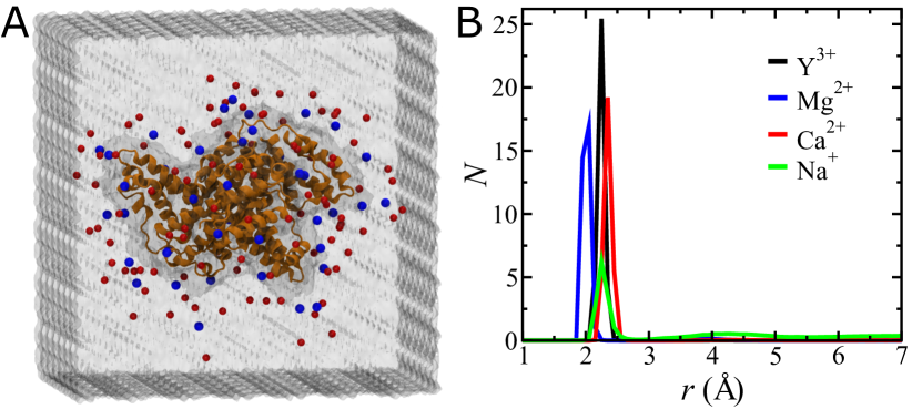
Fig.  1: (A) Snapshot for the starting simulation box (of size 13.2$\times$13.2$\times$13.1 nm³) containing a single BSA protein in 30 mM YCl₃ solution. The protein (orange) is shown in cartoon representation. Y³⁺ (blue) and Cl^- (red) ions are represented as VDW spheres. Water molecules are represented as a continuum in semi-transparent mode for clarity. Note that the system was also simulated in other salt solutions (MgCl₂, CaCl₂, and NaCl) of the same ionic strength as in the case of YCl₃. (B) For each type of cation, the total number of cations $N$ found within shells of width $dr$ $=0.1$ Å, present at a shortest distance $r$ from the protein surface, is plotted as a function of $r$ for the simulation performed at 303 K. $N(r)$ for each cation type is averaged over the last 100 ns of the simulation time. Note that $N(r)$ is enhanced near the protein surface, representing the strong affinity of cations for the negatively charged protein ($-16$ $e$ at pH 7).

To check how tightly the cations are bound to the protein, we monitor their binding/unbinding kinetics. An ion is defined as bound if it is within a cutoff distance $r_{c}$ from any atom of the protein, otherwise the ion is unbound or free. From the $N(r)$ plot in Figure 1B, $r_{c}$${}^{\prime}s$ for the different cations are chosen as 2.8 Å (Na⁺), 2.7 Å (Ca²⁺), 2.3 Å (Mg²⁺), and 2.5 Å (Y³⁺). We find intermittent binding/unbinding events for both Na⁺ and Ca²⁺ ions (Figure S3 in the SI). While the binding/unbinding events for Na⁺ ions are frequent, prolonged bindings are observed for Ca²⁺ ions. For these two cation types, the binding time, i.e., the duration for which an ion remains bound once it comes within distance of $r_{c}$ from the protein, is broadly distributed, owing to the surface heterogeneity of the protein. In contrast, only one unbinding event is observed for Mg²⁺ within 1.27 $\mu$s, whereas no unbinding of Y³⁺ is seen within 1.45 $\mu$s (Figure S3 in the SI). As the water escape time in the first solvation shell of Mg²⁺ is $\sim$1.5 $\mu$s,¹⁵ it presumably requires very long simulations (100 $\mu$s to 10 ms) to obtain sufficient unbinding statistics for Mg²⁺ and Y³⁺ ions. Performing such long, all-atom simulations for our system is out of reach of our computational capabilities.

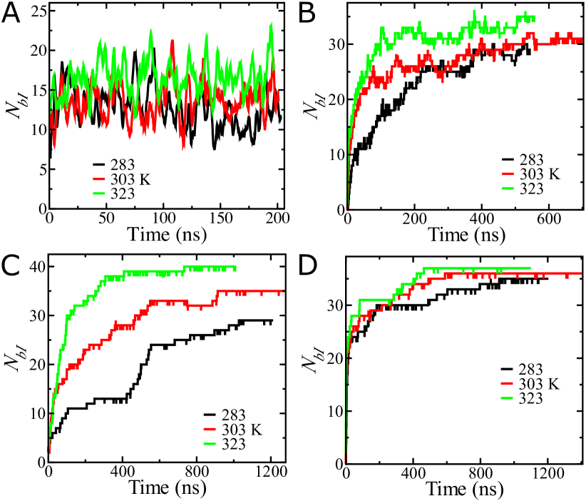
Fig.  2: Time series of the total number of protein-bound cations ($N_{bI}$) at several temperatures for Na⁺ (A), Ca²⁺ (B), Mg²⁺ (C) and Y³⁺ (D) ions. For the multivalent cations, $N_{bI}$ increases upon increasing temperature.

For each cation type, the total number of protein-bound cations, $N_{bI}$, is plotted as a function of the simulation time at three different temperatures in Figure 2. No ion is bound to the protein at the beginning of a simulation, and $N_{bI}$ gradually increases with the simulation time. $N_{bI}$ eventually reaches a saturation value, at a time required for equilibration of the ion distribution around the protein. This ion equilibration time differs for each cation, which can be rationalized by considering the ion–water exchange kinetics that strongly depends on the cation’s charge and size.¹⁵ Counterintuitively, we find from Figure 2 that $N_{bI}$ increases with increasing temperature. This effect is prominent for all the cations, except Na⁺. In contrast, the number of protein-bound water, i.e., the total number of water molecules present within 3 Å from the protein surface decreases with the increase in temperature as expected (Figure S4 in the SI). Although an increase in the binding affinity of any two objects by raising the temperature is not new—e.g., hydrophobic interaction strength increases with temperature,¹⁶ it is surprising to be observed in a system involving strong electrostatic interactions and can be rationalized by the temperature dependence of dielectric and hydration effects.^{17, 18} For a quantitative understanding of this, we calculate various thermodynamic quantities such as the free energy, enthalpy, and various entropy contributions as discussed below.

Thermodynamics of Cation Binding to the Protein

The free energy of a cation binding to the protein, $\Delta G_{b}$, for temperatures in the range of 283–323 K is shown in Figure 3A (see Methods for the calculation details). For each cation type, $\Delta G_{b}$ is always negative, and its magnitude increases with the increase in temperature. $|\Delta G_{b}|$ follows the trend: Na⁺ < Ca²⁺ $\approx$ Mg²⁺ < Y³⁺. By changing temperature from 283 K to 323 K, we see the highest change in $\Delta G_{b}$ for Y³⁺ ($-1.21$ kcal/mol), whereas the least change is observed for Na⁺ binding ($-0.52$ kcal/mol). The changes in $\Delta G_{b}$ for Ca²⁺ and Mg²⁺ ions are $-0.71$ and $-1.03$ kcal/mol, respectively.

The increase in binding affinity of the cations with solely increasing temperature (Figure 3A) cannot be explained by considering the energy of binding, for purely thermodynamic reasons, as described in the SI, section 1. Further, it should be noted that since the dielectric constant of water decreases as $\sim T^{-3/2}$, any electrostatic interaction in water is predominantly entropic in nature.^{17, 18} Therefore, entropy must be playing a dominant role here.

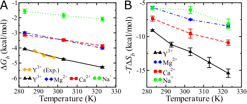
Fig.  3: Temperature dependence of (A) the free energy, $\Delta G_{b}$, and (B) the total entropy contribution, $-T\Delta S_{b}$, for each cation binding to the protein. Error bars represent the standard deviation. The different lines are for guiding the eye. The experimental binding free energies for Y³⁺ at different temperatures shown in (A) are taken from Ref.⁹

The binding free energy for an ion is given by

$$\Delta G_{b}(T)=\Delta E_{b}(T)-T\Delta S_{b}(T),$$ (1)

where $\Delta E_{b}$ and $\Delta S_{b}$ are the energy and entropy of binding, respectively and $T$ is the temperature. For the calculation of $\Delta S_{b}$, one needs to correctly account for “hydration effects” associated with the ion binding process, such as partial desolvation of both the protein and ion. The radial distribution functions for water molecules around a cation, both free in solution and bound to the protein surface, clearly show partial dehydration of the first and second solvation shells (SS${}^{\prime}s$) of each cation (Figure S5 in the SI). $\Delta S_{b}$ in Eq. 1 consists of three terms—the loss in entropy of a protein-bound ion ($\Delta S_{P,I}$), the gain in entropy due to release of tightly-bound water molecules from the first and second SS${}^{\prime}s$ of the ion ($\Delta S_{I,W}$), and the gain in entropy of water molecules released to the bulk due to desolvation of the protein surface residue where the ion binds ($\Delta S_{P,W}$). Together, it can be written as

$$\Delta S_{b}=\Delta S_{P,I}-\Delta S_{I,W}-\Delta S_{P,W}.$$ (2)

We have used the two-phase thermodynamic (2PT) method^{19, 20, 21} to calculate all the terms on the right hand side of Eq. 2. The theory of the 2PT method is described in the SI, section 2 and calculation details are given in the Methods section. We first validate the 2PT method for ionic solutions by reproducing from the simulation data the experimental ion hydration entropy ($\Delta S_{hyd}$) for the different ion types (see Table S1 in the SI). Then, we proceed, using 2PT, with calculations of the entropy differences for a protein-bound ion, a protein-bound water, and a water in the first SS of the cation as shown in Figure 4, as well as the entropy difference of a water in the second SS of the cation as shown in Figure S6 in the SI. Note that for calculations of the various entropy contributions shown in Figures 4 and S6, the reference values are taken as the respective absolute entropies in the bulk water. $\Delta S_{I,W}$ in Eq. 2 is then calculated by multiplying the per water entropy differences with the corresponding numbers of water molecules released in the partial dehydration of both the first and second SS${}^{\prime}s$ of the cation (values given in Table S2 in the SI), and adding both terms. Similarly, $\Delta S_{P,W}$ in Eq. 2 is evaluated by multiplying the per water entropy difference with the number of water molecules released in the partial dehydration of the protein surface residue (values given in Table S2 in the SI). From Figure 4, we see that the entropy loss of a protein-bound cation is more than compensated by the entropy gain of water molecules released to bulk by the partial dehydration of both the cation and protein. The cation desolvation entropy contributes the highest to the thermodynamics of protein–ion binding for all the multivalent cations, whereas both the protein and ion desolvation entropies contribute equally for Na⁺ binding.

The total entropy contribution ($-T\Delta S_{b}$ in Eq. 1) for each cation plotted in Figure 3B is always negative, and it decreases (becomes more negative) with increasing temperature. We have also estimated $-T\Delta S_{b}$ from the temperature dependence of $\Delta G_{b}$ using the thermodynamic relation $\Delta S_{b}=-\partial\Delta G_{b}/\partial T$, and we find that the temperature dependence trend is the same as obtained from the 2PT method, though the values obtained from both methods match only semi-quantitatively (see Figure S7 in the SI for comparison). For each cation, $-T\Delta S_{b}$ is more negative than the binding free energy $\Delta G_{b}$ throughout the temperature range studied in this work (Figure 3). Therefore, the process of a cation binding to the protein is entropy driven. The above observations, in particular, explain the enhancement of the protein-binding affinity of a multivalent cation with increasing temperature (Figure 2). The total entropy contribution as shown in Figure 3B is the highest for Y³⁺ across the whole temperature range, followed by Ca²⁺ > Mg²⁺ $\approx$ Na⁺—representing a delicate dependency of entropy on the charge and size of a cation. Note that though the entropy contribution due to a water molecule released from Mg²⁺ is more than that for Na⁺ and Ca²⁺ ions (Figure 4), the altered trend in $\Delta S_{b}$ for Mg²⁺ in Figure 3B is rationalized by the lower number of water molecules released in the process of a Mg²⁺ ion binding, compared to that for Na⁺ and Ca²⁺ bindings.

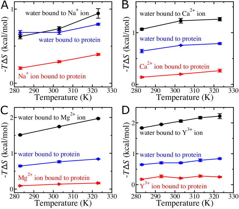
Fig.  4: Entropy contributions $\Delta S_{P,I}$ (red), $\Delta S_{I,W}$ (black), $\Delta S_{P,W}$ (blue) from Eq. 2 as a function of temperature for the protein in NaCl (A), CaCl₂ (B), MgCl₂ (C), and YCl₃ (D) solutions. Error bars represent the standard deviation. The lines are for guiding the eye.

The large (and negative) value of the entropy contribution, $-T\Delta S_{b}$, must be partially compensated by a positive binding energy $\Delta E_{b}$ to result in a small (and negative) value of the binding free energy $\Delta G_{b}$. $\Delta E_{b}$, calculated by using the thermodynamic relation given in Eq. 1, is plotted as a function of temperature in Figure S8 in the SI. $\Delta E_{b}$ is positive throughout the temperature range, in agreement with the experiment,⁹ but is comparable to the magnitude of $-T\Delta S_{b}$. The increase in $\Delta E_{b}$ with temperature (Figure S8) can be rationalized by the enhancement in the electrostatic interaction strength due to the decrease in the water dielectric constant $\epsilon$, as explained below.¹⁷ The electrostatic free energy $\Delta G\propto\epsilon^{-1}$ and $\epsilon\propto T^{-\alpha}$, thus $\Delta G=-CT^{\alpha}$. Here $C$ is a constant and the negative sign is due to $\Delta G<0$ in our case. The entropy follows as $\Delta S=-\partial\Delta G/\partial T=C\alpha T^{\alpha-1}$. The internal energy results as $\Delta E=\Delta G+T\Delta S=-CT^{\alpha}+C\alpha T^{\alpha}=C(\alpha-1)T^{\alpha}$. As long as the exponent $\alpha>1$, $\Delta E$ is always positive and increases as $T^{\alpha}$. For pure water $\alpha>1$ at all temperatures (Figure S9 in the SI). Although $\alpha$ slightly decreases with the addition of salt (viz. 1 M NaCl solution in Figure S9), $\alpha$ is significantly greater than 1 for the temperature regime investigated in our simulations, which explains the observed increase in $\Delta E_{b}$ with increasing temperature.

The temperature-dependent increase in $\Delta E_{b}$ follows the trend: Y³⁺ > Ca²⁺ > Na⁺ $\approx$ Mg²⁺ (Figure S8 in the SI). By changing temperature from 283 K to 323 K, the change in $\Delta E_{b}$ for Na⁺, Ca²⁺, Mg²⁺, and Y³⁺ is found to be 1.82, 2.86, 1.71, and 5.11 kcal/mol, respectively.

The large value of $\Delta E_{b}$ can be understood by considering the energetic penalties associated with the desolvation of both the protein and cation. For example, $\Delta E_{b}$ for Y³⁺ ion at 300 K decreases from 7.50 to 3.71 kcal/mol if we exclude the contribution due to the dehydration of the second SS of Y³⁺ (Figure S10B in the SI). Figure S10 also highlights that the effect of the second SS is significant for the accurate description of solvation thermodynamics of cations, and cannot be neglected even for monovalent ions, e.g., Na⁺.

Preferential Interaction Coefficients

The interaction of ions with proteins, whether these are enriched or depleted from the protein surface, can be quantified by experimentally measuring the preferential interaction coefficient $\Gamma_{23}$. The thermodynamic definition of $\Gamma_{23}$ is the change in chemical potential of the protein due to the addition of ions; it can also be expressed as the change in ion concentration to maintain constant chemical potential when a protein is added to the solution:²²

$$\Gamma_{23}=-\left(\frac{\partial\mu_{2}}{\partial\mu_{3}}\right)_{m_{2},T,P}=-\left(\frac{\partial m_{3}}{\partial m_{2}}\right)_{\mu_{3},T,P},$$ (3)

where $\mu$ is the chemical potential, $m$ is the molal concentration, and the subscripts 1, 2, and 3 stand for water, protein, and ion, respectively. Record et al.,²³ based on the molal concentration definition, developed a two-domain molecular model for the estimation of $\Gamma_{23}$ in terms of the difference in ion concentration in the local domain near the protein surface and the bulk solution as follows:

$$\Gamma_{23}=\bigg{\langle}N_{3}^{local}-N_{1}^{local}\bigg{[}\frac{N_{3}^{bulk}}{N_{1}^{bulk}}\bigg{]}\bigg{\rangle},$$ (4)

where $N_{i}$ is the number of molecules of type $i$ and $\langle\cdot\rangle$ represents the time average. For the calculation of $\Gamma_{23}$ using Eq. 4 a boundary or a distance cutoff needs to be chosen for defining the local and bulk domain, but the choice is arbitrary. $\Gamma_{23}$ is instead estimated at each value of $r$, the distance from the protein surface, asuming that it is the boundary: $\Gamma_{23}(r)=\langle N_{3}(r)-N_{1}(r)[N_{3}^{bulk}/N_{1}^{bulk}]\rangle$. The distance $r^{*}$ after which $\Gamma_{23}(r)$ becomes constant is defined as the actual boundary. In our simulations the total numbers of water molecules ($N_{1}$) and ions ($N_{3}$) are constant, thus the above expression for $\Gamma_{23}(r)$ is further simplified as:²⁴

$$\Gamma_{23}(r)=\bigg{\langle}N_{3}(r)-N_{1}(r)\bigg{[}\frac{N_{3}-N_{3}(r)}{N_{1}-N_{1}(r)}\bigg{]}\bigg{\rangle}.$$ (5)

In a salt solution, cations and anions are distributed around the protein. We obtain preferential interaction parameters for the cation $\Gamma_{2,+3}(r)$ and anion $\Gamma_{2,-3}(r)$ separately by using $N_{+/-3}(r)$ as the cation or anion distribution, respectively in Eq. 5. $\Gamma_{2,+3}(r)$ and $\Gamma_{2,-3}(r)$ are shown for different salt solutions in Figure 5. Experimentally, it is impossible, however, to separate the cationic and anionic contribution to the measured value of $\Gamma_{23}$ for a salt solution. For a salt of monovalent cation and anion, the preferential interaction parameter is given by²³

$$\Gamma_{23}=\frac{1}{2}\big{(}\Gamma_{2,+3}+\Gamma_{2,-3}-|Q_{2}|\big{)},$$ (6)

where $|Q_{2}|$ is the protein’s net charge that is subtracted from $\Gamma_{23}$, as $Q_{2}$ counterions (cations in case of BSA protein) are accumulated near the protein surface to neutralize its charge and do not contribute to the preferential interaction. For a salt of multivalent cation/anion, it is straight-forward to generalize Eq. 6 by scaling $\Gamma_{2,+3}(r)$, $\Gamma_{2,-3}(r)$, and $Q_{2}$ with valency of the anion $z_{-}$, valency of the cation $z_{+}$, and charge on the counterion $z_{+}$, respectively.

$$\Gamma_{23}=\frac{1}{2}\bigg{(}\frac{\Gamma_{2,+3}}{z_{-}}+\frac{\Gamma_{2,-3}}{z_{+}}-\frac{|Q_{2}|}{z_{+}}\bigg{)}.$$ (7)

For the BSA protein, using in Eq. 7 $\Gamma_{2,+3}$ and $\Gamma_{2,-3}$ at $r^{*}=17$ Å (by which all curves reach their respective saturation values as seen in Figure 5), we obtain preferential interaction coefficients for different salts: NaCl ($\Gamma_{23}=2.44$), CaCl₂ ($\Gamma_{23}=15.67$), MgCl₂ ($\Gamma_{23}=19.83$), and YCl₃ ($\Gamma_{23}=26.87$). Positive values of $\Gamma_{23}$ for all the different salt types reflect that these salt ions are attracted towards the protein surface. For salt containing multivalent ions, $\Gamma_{23}$ is significantly larger than that for NaCl, which suggests that addition of trivalent ions in the protein solution affects the solution stability²⁵ and stabilizes protein dimer formation as seen in our simulations.

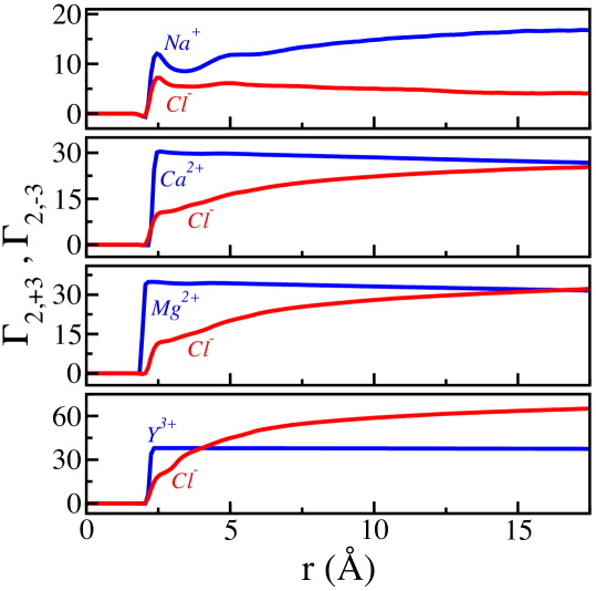
Fig.  5: Preferential interaction coefficients for cations $\Gamma_{2,+3}$ and anions $\Gamma_{2,-3}$ of the different salt solutions at 303 K as a function of the boundary distance cutoff $r$. $\Gamma_{2,+3}(r)$ reaches a saturation value rather quickly compared to $\Gamma_{2,-3}(r)$, for solutions containing multivalent cations.

$\zeta$-Potential of the Protein and the Protein–Protein Interaction

$\zeta$-potential measurements for a protein in an ionic solution report on charge compensation by the counterions and thus have direct implications for protein–protein association and the phase behavior of the solution. $\zeta$-potentials are defined by the electrophoretic mobility.^{10, 9, 26} From the simulation data, we calculate the surface potential at one ionic diameter away from the protein surface (see Methods). Note that the surface potential typically serves as a good approximation for the $\zeta$-potential for proteins and colloidal systems; however, the surface and $\zeta$-potential values might differ significantly for extended surfaces with high surface charge densities.²⁷

As shown in Figure 6, the $\zeta$-potential of the protein in the NaCl solution is negative at all temperatures, as expected based on the protein net charge of $-16$ $e$. In contrast, the $\zeta$-potential is positive for all multivalent cation-chloride solutions at all temperatures, indicating sign reversal of the effective charge of the protein (Figure 6). This charge inversion phenomenon in the presence of multivalent cations is due to strong interactions of the cations predominantly with the COO^- groups of the protein’s surface residues and can be rationalized by considering strong charge-charge correlations.²⁸ Note that similar charge reversal of proteins in the presence of trivalent cations has also been reported both in experiments^{4, 26, 9} and simulations¹³ as well as in a coarse-grained analytical model.²⁹ As shown in Figure 6, with the increase in temperature, the $\zeta$-potential of the protein increases for all cation types; the highest change is seen for MgCl₂, whereas the effect is minimal for NaCl. The $\zeta$-potential of the protein at 283 K is higher in CaCl₂ solution than in MgCl₂ solution, and vice versa at 323 K. These observations are consistent with the trends for the temperature dependence of binding free energies of the different cations (Figure 3A).

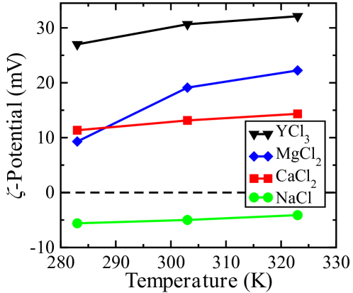
Fig.  6: Temperature dependence of the $\zeta$-potential of the protein in various salt solutions. The lines are guide to the eye only.

Protein–Protein Binding Mediated by Cation Bridges

Protein aggregation seen in experiments⁹ was hypothesized to be mediated by cation bridges.⁶ To explicitly demonstrate the multivalent ion-mediated protein–protein binding, we have performed three independent simulations with different orientations of two BSA proteins in YCl₃ solution, as shown in Figure 7A (left panel). In every simulation, we find that two BSA proteins, which are initially placed far apart, approach each other (see the timeseries of the total number of inter-protein residue–residue contacts in Figure 7B) and eventually form a dimer mediated by 1–5 Y³⁺ ions (see snapshots in Figure 7A [middle panel]). The Y³⁺ ion bridges remain stable over a 1 $\mu$s timescale, as evident from the time series plot for the number of bridging cations (Figure 7C). A Y³⁺ ion bridge is stabilized by coordination of multiple caboxylate groups of each protein with the cation, as evident from snapshots in Figure 7A (right panel). Note that even for the stable, Y³⁺ ion-bridged protein dimer complex, the relative orientation between the two proteins changes over time but very slowly (see the orientational autocorrelation function in Figure 7D). This reveals the conformational flexibility of the protein dimer complex.

To compare monovalent and multivalent cations, we have also simulated the above three systems (shown in Figure 7A) in NaCl solution, at the equivalent ionic strength as for YCl₃ solution. In sharp contrast to the case of YCl₃, we find that Na⁺ ion bridges between two BSA proteins form transiently and remain stable only for 1–20 ns (Figure 7E). These results demonstrate the need for multivalent ions in protein cluster formations, in agreement with experiments.⁴

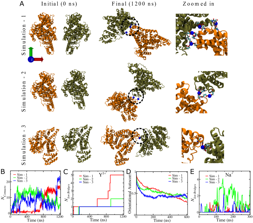
Fig.  7: Results for two BSA proteins (A–D) in 30 mM YCl₃ and (E) 180 mM Nacl solution at 303 K. (A) The initial and final configuration of two BSA proteins (represented in orange and tan). Bridging Y³⁺ ions in the final structure are shown as blue spheres, and amino acid residues of the two proteins involved in the formation of ion bridges are highlighted in the ball–stick representation (see the right panel for the zoomed-in version). Water and other ions are omitted for clarity. (B) Time series of the total number of inter protein residue–residue contacts. (C) Time series of the total number of Y³⁺ ion bridges that link the two proteins to form a dimer. (D) The average autocorrelation function for the relative orientation angles between the principal axes of two proteins as a function of time delay. (E) Time series of the total number of Na⁺ ion bridges that form transiently between two BSA proteins in 180 mM NaCl solution at 303 K. All observables are defined in Methods.

Discussion

The temperature behavior of the $\zeta$-potential found in Figure 6 is in qualitative agreement with the experiments.⁹ As the $\zeta$-potential is influenced by the number of surface-bound ions and the binding affinity of ions increases with temperature, the $\zeta$-potential is expected to increase with temperature irrespective of the salt concentration of the solution. $\zeta$-potential values estimated from our simulations, however, are larger than that reported in the experiments⁹ presumably because of the YCl₃ concentration difference. The $\zeta$-potential increases with increasing YCl₃ concentration as found in experiments,⁹ thus we expect the simulation and experimental results to match if the same salt concentration is used.

It should be noted that the YCl₃ concentration used in our simulations is 30 mM which is much higher than the 1 mM concentration used in the experiment. A direct comparison between all-atom simulations and the experiments⁹ at low concentration of multivalent ions is rather difficult for the following reason. We consider a higher YCl₃ ion concentration in our simulations in order to obtain statistically converged results with sufficient number of ions. Obtaining well-converged results for proteins at low salt concentrations with enough number of ions would require significantly larger system sizes. Simulating such large systems is very demanding at the all-atom level, but it is feasible at a coarse-grained level as shown in a recent study.¹³ However, the solvation effects, which are crucial for the accurate prediction of protein–ion binding thermodynamics, are not properly taken into account in such coarse-grained simulations.

The LCST phase behavior found in experiments⁹ can be rationalized by the temperature dependence of the $\zeta$-potential and the microscopic picture emerges from our simulations. For sufficiently low Y³⁺ concentration, at low temperatures due to the reduced binding affinity of counterions, the $\zeta$-potential is expected to become negative (and large) and the proteins are expected to repel each other, keeping the solution stable. With increasing temperature, counterion binding affinity for the protein increases, and hence the $\zeta$-potential increases and becomes positive at a sufficiently high temperature. In the temperature range (293–313 K) where the $\zeta$-potential is small ($-$5 to $+$5 mV),⁹ the proteins are predicted to attract each other, eventually causing the solution to phase separate into protein-rich and protein-poor phases.

The protein–protein binding at a low concentration of multivalent ions occurs via cation bridging, as shown in Figure 7, as well as suggested from experiments.^{6, 9} A cation bridge formation—like the first step of a cation binding to the protein—requires desolvation of both the protein-bound cation and the surface residue of another protein that will bind to the cation. These processes involve the release of many tightly-bound water molecules to the bulk that results in a significant entropy gain, which contributes at least 10–15 kcal/mol (depending on the temperature) to the total free energy, as shown in Figure 3B for a Y³⁺ ion binding. As multiple cation bridges are formed in a protein–protein binding (see Figure 7, and also found in experiments⁶), the net entropy gain due to cation and protein desolvation more than compensates for the translational and rotational entropy losses of the proteins during protein–protein binding. Therefore, the LCST phase behavior⁹ is entropy-driven.

Conclusions

In summary, by performing fully atomistic MD simulations of a BSA protein in different cation-chloride solutions (NaCl, CaCl₂, MgCl₂, and YCl₃) and by calculating various entropy contributions, we demonstrate that multivalent cation binding to the protein is an entropy-driven phenomenon. The loss in entropy of a protein-bound cation is more than compensated by the entropy gain of water molecules due to the partial dehydration of both the cation and the cation-bound surface residue of the protein. A particularly interesting observation is the significant difference in the binding/unbinding kinetics of Ca²⁺ and Mg²⁺ ions (see Figure S3)—although having comparable binding free energies (Figure 3A), which can be related to the recent finding that the ion–water exchange kinetics strongly depends on the size of a cation.¹⁵ It will thus be interesting to investigate in future simulation studies the universality of the ion size dependence of ion–protein binding kinetics and thermodynamics.

The $\zeta$-potential calculation shows charge inversion of the protein in all solutions containing multivalent cations, but not in the monovalent NaCl solution (Figure 6). The LCST phase behavior observed in the experiment⁹ can be rationalized by considering the temperature-dependent increase in the $\zeta$-potential of the protein and the associated charge inversion phenomenon. The protein–protein interaction involves: (i) the ion binding to the protein, and (ii) the subsequent protein–protein binding by cation bridging (Figure 7). In both processes many tightly-bound water molecules are released to the bulk, which results in a thermodynamic driving force for the LCST behavior that is entropic in nature, in agreement with the experiment.⁹

This work shows that similarly to hydrophobic association, entropy plays a pivotal role in systems involving strong electrostatic interactions, revealing intriguing hydration and dielectric effects. Our results are important for the basic understanding of ion effects in soft matter and biology, and the insights gained here will be useful in studies of ion-mediated surface adsorption and crystallization of proteins. Moreover, molecular-level understanding of interactions of heavy metals—usually not found in healthy cells—with different biomolecules, as studied here, can provide insights for carcinogenicity and neurotoxicity induced by exposure to such environmental contaminants.

Methods

Model Building and Force Field Parameters

The initial structure of BSA protein was obtained from the crystal structure available in the protein data bank (PDB ID: 3V03). The charge or protonation state of each residue of the protein was chosen at neutral pH 7 depending on the residue’s pK_a value, and the assigned charges were fixed over the simulation time. Note, however, that pK_a depends on the ionic strength (through the activity coefficients), and the reported pK_a values of amino acids are typically determined in a solution of high ionic strength.³⁰ In particular, the apparent pK_a values of carboxyl groups shift up slightly in the presence of multivalent cations at low salt concentrations. If the pH of the solution differs from 7 in an experiment due to the CO₂ content in air (which lowers the water pH down to 5.6 ³¹), this could make some of the acidic peptide groups less charged. But, the experiments described in Matsarskaia et al.⁹ were performed in air and in ultrapure (MilliQ, 18.2 Mega Ohm) water which had previously been degassed under vacuum to eliminate the CO₂ contributions. Also, it is known from experiments that the addition of multivalent metal cations such as Al³⁺ and Fe³⁺ changes the pH of the solution due to hydrolysis of these cations, which can change the charge states of the protein surface residues. However, this effect is less significant for Y³⁺ ion.¹⁰ Therefore, our assigned fixed charges of the protein residues at pH 7 for the different cations (Na⁺, Ca²⁺, Mg²⁺, and Y³⁺) is assumed to mimic the experimental conditions sufficiently well.

The ff14SB force field parameters³² were used for the protein. The system was solvated with TIP3P³³ water model using the xleap module of the AMBER17 tools³⁴ in a way such that there exists at least 17 Å solvation shell in between the solute and simulation box wall. The final unit shell for simulation is a rectangular box of size 13.2$\times$13.2$\times$13.1 nm³ that contains $\sim$200,000 atoms (Figure 1A). The system was simulated in four different salt solutions, namely NaCl, MgCl₂, CaCl₂ and YCl₃. Depending on the ion type, an appropriate number of counterions were added to ensure the charge neutrality of the simulation unit shell. To simulate the system at a specified salt concentration, enough numbers of counterions/coions, estimated from the mole fraction of counterions/coions and water, were further added to the system. For YCl₃, the system was simulated at 30 mM salt solution. For the other salts, the system was simulated at the equivalent ionic strength as in the case of YCl₃, e.g., 180 mM for NaCl. Especially for multivalent ions, the electronic polarization effect contributes significantly to the total interaction energy of such an ion with another charged object. The recently developed Li/Merz ion parameters^{35, 36, 37} with 12-6-4 Lennard-Jones (LJ)-type nonbonded interaction terms take care of the electronic polarization effect and have been shown to well reproduce the experimental measurables, such as the ion–oxygen (of water) distance, the ion–water coordination number, and the hydration free energy of mono- and multi-valent ions. We have provided in Table S1 in the SI the structural parameters and entropy of ion hydration for the different ions calculated from our simulation data, which quantitatively match with the corresponding experimental values. Therefore, we used Li/Merz ion parameters for an accurate modeling of the ion–water and ion–protein interactions.

MD Simulation Details

All the simulations were performed using the PMEMD module of the AMBER14 package.³⁸ Periodic boundary condition was used for all the simulations. Bonds involving hydrogen atoms were constrained using the SHAKE algorithm³⁹ that allowed the use of a time step of 2 fs for the integration of Newton’s equation of motion. The temperature of the system was maintained using a Langevin thermostat⁴⁰ with the collision frequency of 5.0 ps^-1. Berendsen weak coupling method⁴¹ was used to apply a pressure of 1 atm with isotropic position scaling with a pressure relaxation time constant of 2.0 ps. Particle mesh Ewald⁴² sum was used to compute long-range electrostatic interactions with a real space cutoff of 10 Å. van der Waals and direct electrostatic interactions were truncated at the cutoff. The direct sum non-bonded list was extended to cutoff + “nonbond skin” (10 + 2 Å).

The solvated systems with harmonic restraints (force constant of 500 kcal/mol/Ų) on the position of each atom of the protein were first subjected to 2000 steps of steepest descent energy minimization, followed by 1000 steps of conjugate gradient minimization to remove bad contacts present in the initially built systems. The restraints on the protein atoms were sequentially decreased to zero during further 4000 steps of energy minimization. The energy minimized systems were then slowly heated from 10 K to the desired temperature in many steps during the first 210 ps of MD simulation. During this time, the solute particles were restrained to their initial positions using harmonic restraints with a force constant of 20 kcal/mol/Ų. The first 2 ns of equilibration simulations were performed in the NPT ensemble to attain the proper water density. Simulations were then switched to the NVT ensemble for further production runs of 200–1450 ns, depending on cation types.

Data Analysis

All the analyses were carried out by using home-written codes and/or the AMBER17 tools.³⁴ Images were rendered using the Visual Molecular Dynamics software.⁴³

The free energy of ion binding, $\Delta G_{b}$, was calculated using the expression

$$\Delta G_{b}=-k_{B}T\ln(C_{bI}/C_{fI}),$$ (8)

where $k_{B}$ is the Boltzmann constant, and $C_{bI}$ and $C_{fI}$ are the concentration of bound and free ions, respectively. The expressions for calculations of the concentrations are $C_{bI}=N_{bI}/V_{s}$ and $C_{fI}=N_{fI}/V_{f}$, where $V_{s}$ is the volume of the shell around the protein surface where ions are considered as bound, $N_{fI}$ (= total number of ions $-N_{bI}$) is the number of free ions, and $V_{f}$ is the free volume available for ions. The volumes were calculated following the protocol described in Ref. ⁴⁴, by using the Gromacs program gmx sasa.⁴⁵ Further details on the volume calculation are provided in the SI, section 3. The last 200 ns data for each ion type (the last 150 ns for Na⁺) was taken for the calculation of $\Delta G_{b}$, whereas the rest of the data served for the equilibration.

The reported entropy contributions in Figures 4 and S6 were obtained by calculating absolute molar entropies for free and protein-bound ions, free and protein-bound water molecules, and water molecules in the first and second SS${}^{\prime}s$ of the cation by using the 2PT method.^{19, 20, 21} To generate trajectories for 2PT calculations, simulations were restarted after 100–500 ns, depending on the ion type. 3 short (40 ps) NVT trajectories for each system at each temperature were generated with coordinates and velocities saved every 4 fs. To calculate the 2PT entropy for bound ions, we performed the analysis for all bound ions and got the average entropy per ion, similarly for bound water. In Figures 4 and S6, each point and the corresponding error bar are the average and standard deviation of 3 different simulations, respectively.

The surface or $\zeta$-potential was obtained by calculating as a function of $r$ (the distance from the center of mass of the protein) the electrostatic potential profile, $\phi(r)$, for the system as follows.⁴⁶ $\phi(r)$ was calculated by solving the Poisson equation, i.e, by carrying out a double integration of the charge density profile, $\rho(r)$, obtained from our MD simulation by using the following expression.

$$\phi(R)-\phi(r)=-\frac{1}{\epsilon}\int_{r}^{R}dr_{1}\frac{1}{r_{1}^{2}}\int_{0}^{r_{1}}dr_{2}r_{2}^{2}\rho(r_{2}),$$ (9)

where $R$ (= 65 Å) is the radius of the inscribed sphere within the rectangular MD simulation box and $\epsilon$ is the dielectric permittivity of water. A derivation of Eq. 9 is given in the SI, section 4. At a temperature $T$, $\epsilon$ was calculated from the Bjerrum length, $\lambda_{B}$, of water (= 7 Å) by using the relation: $\epsilon=e^{2}/4\pi\lambda_{B}k_{B}T$, where $e$ is the elementary charge. It should, however, be noted that for the temperature behavior of $\epsilon\propto T^{-\alpha}$, the exponent $\alpha$ in experiments is close to ${}^{3}/_{2}$ but we take it to be 1 which is close to what is seen in simulations for a rather similar water model.¹⁸ So the above approximation for $\epsilon(T)$ is deemed to be good for our purpose. Finally, the $\zeta$-potential was obtained as $\zeta=\phi(R)-\phi(R_{h}+2r_{c})$. Here, the hydrodynamic radius of the protein, $R_{h}$, was taken to be 36 Å,⁴⁷ and $r_{c}$${}^{\prime}s$ for the different cations (Figure 1B) were taken to be 2.8 Å (Na⁺), 2.7 Å (Ca²⁺), 2.3 Å (Mg²⁺) and 2.5 Å (Y³⁺).

$N_{Contacts}$ shown in Figure 7B is defined as the total number of inter-protein amino acid residue–residue contacts, and such a contact is counted if at least one pair of atoms from residues of two different proteins are within 3 Å.

$N_{IonBridges}$ shown in Figure 7C is defined as the total number of ions bridging two different proteins, and an ion bridge is counted if an ion is present within 3 Å from both the proteins’ surfaces.

The average orientational autocorrelation function shown in Figure 7D is defined as

$$C(t)=\frac{1}{3}\sum_{i=1}^{3}\frac{\langle\cos\theta_{i}(0)\cdot\cos\theta_{i}(t)\rangle}{\langle\cos\theta_{i}(0)\cdot\cos\theta_{i}(0)\rangle},$$ (10)

with $\cos\theta_{i}(t)=\hat{e}_{i}^{A}\cdot\hat{e}_{i}^{B}$, where $\hat{e}_{i}^{A}$ and $\hat{e}_{i}^{B}$ are the unit vectors along the principal axes of proteins A and B, respectively, and the angular bracket represents the average over time origins.

Conflicts of interest

There are no conflicts to declare.