Real-time Bidding for Time Constrained Impression Contracts in First and Second Price Auctions – Theory and Algorithms

Abstract

We study the optimal behavior of a bidder in a real-time auction subject to the requirement that a specified collections of heterogeneous items be acquired within given time constraints. The problem facing this bidder is cast as a continuous time optimization problem which we show can, under certain weak assumptions, be reduced to a convex optimization problem. Focusing on the standard first and second price auction mechanisms, we first show, using convex duality, that the optimal (infinite dimensional) bidding policy can be represented by a single finite vector of so-called “pseudo-bids”. Using this result we are able to show that, in contrast to the first price auction, the optimal solution in the second price case turns out to be a very simple piecewise constant function of time. Moreover, despite the fact that the optimal solution for the first price auction is genuinely dynamic, we show that there remains a close connection between the two cases and that, empirically, there is almost no difference between optimal behavior in either setting. Finally, we detail methods for implementing our bidding policies in practice with further numerical simulations illustrating the performance.

Keywords

Real-time Bidding; Infinite-dimensional Optimization; Computational Advertising; Auction Theory; First Price Auction; Second Price Auction; Transportation Production Problem

Acknowledgement

We acknowledge the support of the Natural Sciences and Engineering Research Council of Canada (NSERC), [funding reference number 518418-2018]. Cette recherche a été financée par le Conseil de recherches en sciences naturelles et en génie du Canada (CRSNG), [numéro de référence 518418-2018].

1 Introduction

Since at least 2016 online advertising, which includes ads in cellphone apps, website banner ads, search engine keyword ads, etc. has been the dominant advertising segment [19]. One of the drivers of this dominance is not only the fact that so many people are now online, but that the technology enables more accurate targeting. That is, advertisers can accurately target their messaging to the groups or individuals to which the message is most relevant. This technology enables advertisers to raise awareness of their products, website or app operators (i.e., “publishers”) to monetize their audiences, and internet users to access a wealth of gratis content.

There are many different mechanisms through which publishers can sell ad space. For example, sponsored search is a well known mechanism for search engines where certain keywords (e.g. “mortgage”, “used car”, etc.) trigger the display of relevant sponsored results. More traditional fixed contracts (e.g., for the display of fixed banner ads) between advertisers and publishers also remain common, particularly for businesses which need to be careful about their image and want to maintain complete control over what their brand is associated with. Finally, a significant portion of total advertising revenue is generated through a mechanism called real-time bidding (RTB), which is the mechanism at the focus of this paper.

RTB is facilitated by auction exchanges (e.g., Google AdX [28]) where the arrival of each user to a publisher website or app triggers a sealed-bid auction (the bid is hidden from other participants) wherein advertisers bid on the right to display their ad to the particular user. Generically, we will think of this as a single “item”, and the known characteristics (e.g., age, interests, etc.) of the visitor as the item’s “type”. Advertisers decide upon which types they wish to target, and bid on these items when they arrive at the auction exchange.

In this paper we study a problem of interest to intermediaries or brokers known as Demand Side Platforms (DSPs), see e.g. [39]. Advertisers contract with these DSPs to bid on the RTB market on their behalf. Specifically, we consider DSPs that have entered into contracts which require a specified number of items of particular types be won within a given time deadline. We do not allow for the contract requirements to be subject to post hoc negotiation – once the contract is accepted the DSP is obligated to meet the requirements. This benefits the advertiser by allowing them to offload the risk associated with price changes in the market, and gives the DSPs the opportunity to profit from managing this risk on behalf of multiple advertisers. Thus, the objective of the DSP is to win the required items in RTB at the lowest possible cost (since the difference between the contract value and its cost of acquiring the ads is the profit). This is a natural setting to consider as there is a reasonable expectation of efficiency gains when the demands of a large number of advertisers are aggregated by intermediaries.

The dominant auction mechanisms in RTB are first price and second price auctions. In either case, the item is awarded to the highest bidder, but the difference lies in what they pay: in a first price auction, the winning bidder pays their actual bid, whereas in a second price auction, the winning bidder pays whatever the second highest bid was. In both auctions, the bids are sealed (other participants don’t observe them, even after an item is allocated) so the only source of information about prices are from available historical data, and the knowledge gained from the bidder’s direct participation. Standard overviews of auction theory are provided by [24, 29].

Related Work

Real-time bidding is commonly studied from at least two main perspectives: the descriptive analysis of the market itself (e.g., [20, 2, 3]), where questions of game theoretic equilibria are at the forefront; and the consideration of normative problems of optimal bidding. Our perspective is normative. We solve an optimal bidding and allocation problem by providing algorithms which produce a plan over a given time horizon specifying the optimal average rate that items should be acquired, and to which contracts (or campaigns) they should be allocated. Similar allocation problems have been considered from the publisher’s viewpoint [8, 33] and the advertiser’s [48, 37]. However, aside from [37], no other papers, to our knowledge, have considered contract management aspects with hard constraints from the DSP perspective. Many works have studied the problem of short time horizon adaptation, for instance the works of [16, 47, 21, 23] have applied classical control theory methods (e.g., PID controllers) and those of [18, 7, 43] MDP formulations and reinforcement learning. The goal of these works are to maintain or maximize certain performance indicators, e.g., click through rates or purchasing decisions. As such, these works can be seen as considering a faster time scale in comparison to our problem. Optimal bidding problems over a long time horizon are considered by [13, 17] via application of stochastic optimal control, where the goal is to maximize the total valuation of items attained over the period, subject to budget constraints. An important consideration has thus also been the estimation of item valuations, and how to map valuations into bids, see e.g., [32, 49]. These are distinct from the present work since we do not appeal to any notion of item valuation, indeed, a valuation can only be derived from the contract requirements. Our formulation is also dual to many of these as we seek to minimize the cost of obtaining a given number of items, as opposed to maximizing the utility of items obtained within a given budget. A similar class of problems to our optimal acquisition problem is that of revenue management (see e.g., [40, 6]) wherein a merchant needs to set prices for their wares in order to optimally liquidate their inventory. Aside from the superficial distinction of sell-side versus buy-side, the contract management problem studied in the present paper involves substantially different constraints. Finally, many papers have also studied separate, but important, statistical estimation problems (e.g. [11, 44, 51, 52, 45, 15]) concerned with estimating the prevailing prices of arriving items.

Contributions

This paper studies an optimal bidding and allocation problem similar to the earlier work of [37] for second price static auctions, but with the additional consideration of temporal dynamics and differing contract deadlines. The main contributions of this paper over those of [37] are threefold: Firstly, the recognition that the problem is in fact naturally convex, this leads to an analysis which is general enough to unify both the first and second price auctions, as well as to result in an insightful duality theory. Secondly, a clear development of practical and simple algorithms for implementing solutions to the optimal bidding and allocation problem are provided, along with detailed simulation evidence and practical methods for adaptation to a stochastic environment. And finally, we show that there is a close connection between the first and second price cases, both theoretically as well as through experimental evidence.

Outline

The outline of the paper is as follows: We formally introduce the problem in Section 2. In Section 2.3, we show that it can be reformulated as an infinite dimensional convex optimization problem (albeit with some additional assumptions in the first price case, see Proposition 2.2). The convex formulation and a strong duality theorem is provided in Section 2.4, where we also show that the optimal time dependent bids are fully determined by a finite set of parameters deemed pseudo bids. Using duality, we show in Section 2.5 that there is a close connection between the first and second price case; this connection is expanded upon in the simulations of Section 3.2, where experimental evidence demonstrates that there is little practical difference between the solutions calculated in the two cases. In terms of implementation, the dual problem in Section 2.4 is finite and can be solved to attain exact solutions, but doing so requires computationally expensive integration steps; this motivates a simpler polyhedral approximation method in Section 3.1, where we also bound the error between the approximation and the true optimal solution. Using the methods of Section 3.1, an empirical study is carried out in Section 3.2 using real RTB data. Motivated by the results of this simulation, Section 3.3 examines additional practical methods for online bid updates and for accounting for uncertainty in any estimated quantities. Finally, Section 4 concludes. Proofs are provided in the appendix.

2 The General Optimal Bidding Problem

We consider the problem of bidding in a sequential auction with $M$ available item types $j\in[M]\overset{\Delta}{=}\{1,2,\ldots,M\}$ and where we are required to fulfill $N$ contracts by winning a specified number of items of given types. Specifically, the contract $i\in[N]$ is a $3$-tuple $(\mathcal{A}_{i},C_{i},T_{i})$, where $\mathcal{A}_{i}\subseteq[M]$ is the set of item types that can be allocated towards the contract, $C_{i}$ is the number of items (of any type in $\mathcal{A}_{i}$) that are needed, and $T_{i}$ is the time deadline by which the items must be obtained. Another collection of sets, $\mathcal{B}_{i}$, is uniquely determined by the condition $i\in\mathcal{A}_{j}\iff j\in\mathcal{B}_{i}$, and the sets $\mathcal{A}_{i},\mathcal{B}_{j}$ therefore determine a bipartite graph $\mathcal{G}$ on $[N]\times[M]$ encoding which item types can be allocated to which contracts, and conversely, which contracts can be satisfied by which item types. It will be convenient to write $(i,j)\in\mathcal{G}$ to mean that $i,j$ is an edge in this graph.

We will suppose without loss of generality that $0<T_{1}\leq T_{2}\leq\cdots\leq T_{N}$. Contracts stipulating more complicated item requirements (e.g., at least $100$ of type $j$, and an additional $50$ of either $j$ or $j^{\prime}$) can be implemented by introducing multiple contracts with the same deadlines. Denoting $T\overset{\Delta}{=}T_{N}$ for the end of the problem horizon and $T_{0}\overset{\Delta}{=}0$ will also be notationally convenient. The time $T_{i}$ indicates when contract $i$ “exits” the problem, and similarly it will be convenient to write $T^{j}=\underset{i\in\mathcal{B}_{j}}{\text{max }}T_{i}$ for the time that items of type $j$ exit, i.e., are no longer needed.

Remark 2.1 (Non-zero Initial Times).

The framework can also incorporate introducing new contracts part way through the fulfillment of existing ones by “resetting” the existing contracts by subtracting the current time and already obtained supply from their requirements, and then adding the new contracts to the collection before recalculating the optimal bids. This is further explored in Section 3.3.1 for the purpose of adapting to a stochastic environment. Managing contracts with starting times other than $0$ is also not a major difficulty: each contract must now come along with a starting time $S_{i}$ and it’s deadline $T_{i}$, the ultimate result being that integrals over the interval $[0,T_{i}]$ would need to be taken over $[S_{i},T_{i}]$, and the dual problem considered in Section 2.4 will have additional variables. In some applications (e.g., processor speed scaling [14]), there are algorithms which can take advantage of special structure in the arrivals of jobs (e.g., that the jobs be first-in first-out: $S_{i}\leq S_{j}\implies T_{i}\leq T_{j}$) to achieve performance improvements, but such structure does not impact the methods we develop here.

Remark 2.2 (Item types).

That a contract may be fulfilled with any arrangement of items in $\mathcal{A}_{i}$ (e.g., $C_{i}$ items of a single type $j\in\mathcal{A}_{i}$ is just as good as an even distribution over all items in $\mathcal{A}_{i}$) appears at first as an unusual modelling artifact. However, it need not be the case that the counter party can distinguish between item types. For example, consider two contracts: contract $1$ targets anyone aged $30-40$, and contract $2$ targets anyone aged $20-40$. This would result in the DSP recognizing two types of items: people aged $20-30$ and people aged $30-40$. Contract $2$ can indeed be fulfilled just as well with either type, but contract $1$ can be fulfilled only with the second type.

2.1 Supply Rate Curves and Cost Functions

The model of how items are acquired relies on a function $W_{j}(x,t)$, called a supply curve, associated to each item type $j$ and quantifying, instantaneously at time $t$, the expected number of items that would be won by bidding $x$. This function derives from the assumption that our bidder is a price taker, i.e., has no substantial market impact.

The function $W_{j}(x,t)$ should be thought of us an un-normalized (cumulative) distribution function with respect to the bid argument $x$, but as a rate with respect to the time argument $t$. This function needs to be estimated from available historical data (see e.g.,  [11, 44, 51, 41, 15] for work on this problem), and represents what is essentially a fluid approximation of the “landscape” of competing bids. It is important to emphasize that these curves represent averages, but that the environment is stochastic in actuality. Assuming that we only have access to the first order average statistics leads to a simpler problem, while at the same time also being a weaker assumption than if we were to develop a full stochastic model that assumes further information about higher order statistics. Nevertheless, we will see in Section 3.3 some practical methods for adapting to the stochastic environment.

We remark that the purpose of including time-dependence is to enable the consideration of forecast changes in supply availability; in particular, there are natural cycles present in the average available supply throughout time: see e.g., [46], as well as Figure 1.

Additionally, we must introduce a cost function $f_{j}(x,t)$ which quantifies, instantaneously at time $t$, the expected cost of bidding $x$ on every arriving item of type $j$. This function naturally depends on the auction mechanism, but also on the supply rate curve $W_{j}$, since the total amount spent depends upon the number of items which are actually won. In order to lighten the notation, we will often suppress the $j$ index and $t$ argument, writing $W(x),f(x)$ etc. when it is clear from, or irrelevant to, the context.

For a first price auction, the cost function is the product of the bid and the supply rate curve, since you pay your bid:

$$f^{1st}(x)=xW(x)\mathbf{1}_{\mathbb{R}_{+}}(x),$$ (1)

where

$$\mathbf{1}_{A}(x)=\left\{\begin{array}[]{lr}1&x\in A\\ 0&\text{otherwise}\end{array}\right.,$$

is the indicator for the set $A$.

In the second price case, the supply rate curve becomes an integrator, since we only pay the highest competing bid:

$$f^{2nd}(x) =\int_{0}^{x}u\mathsf{d}W(u)\mathbf{1}_{\mathbb{R}_{+}}(x)$$ (2)

$$=\bigl{[}xW(x)-\int_{0}^{x}W(u)\mathsf{d}u\bigr{]}\mathbf{1}_{\mathbb{R}_{+}}(x),$$

where the first integral is to be understood as a Lebesgue-Stieltjes integral (see e.g. [36, ch. 6]) and we have integrated by parts. The inequality

$$f^{2nd}\leq f^{1st},$$ (3)

is evident from the above since $f^{2nd}(x)=f^{1st}(x)-\bigl{[}\int_{0}^{x}W(u)\mathsf{d}u\bigr{]}\mathbf{1}_{\mathbb{R}_{+}}(x)$.

We will consider both first price and second price auctions as the two cases are amenable to a unified treatment. However, we often place our focus on the first price case, as its analysis requires an additional (albeit rather weak) assumption. We will occasionally omit the superscript $1st$ or $2nd$ (sometimes written as a subscript) depending on whether or not we want to emphasize a particular case. Moreover, it is important to recognize that the DSP must estimate the curve $W(x)$ in the auction they will actually participate in. Due to strategic differences between the first and second price cases, these functions will not be the same across auction types, but our analysis has no need to distinguish between them.

We make the following basic assumptions.

Assumption 2.1 (Supply Rate Curve Properties).

For every $t\in\mathbb{R}_{+}$, the functions $x\mapsto W_{j}(x,t)$ are strictly positive and continuous on $\mathbb{R}$, as well as being either strictly monotone increasing on an interval $(-\infty,\bar{x}_{j}]\subseteq\mathbb{R}$ and flat thereafter, or strictly monotone increasing on $\mathbb{R}$ and unbounded. Moreover, $\bar{s}_{j}(t)\overset{\Delta}{=}\text{sup}_{x}W_{j}(x,t)$ is either $+\infty$ or attained at some $\bar{x}_{j}(t)\in\mathbb{R}$. Finally, $W_{j}(x,t)\rightarrow 0$ as $x\rightarrow-\infty$.

The reasons for these assumptions, and whether or not they can be relaxed, is discussed in the following sequence of remarks.

Remark 2.3 (Attainment).

That the supremum of $W$ must be obtained when finite is not a benign assumption. It technically excludes many models of the form $W(x,t)=\lambda(t)W(x)$ where $\lambda(t)$ is a supply rate and $W(x)$ is a cumulative distribution function with unbounded support (e.g., $1-e^{-\gamma x}$). Of course, this is essentially only a theoretical restriction, and such models are reasonable in practice since one could choose some large but fixed maximum allowable bid $\bar{x}$ and truncate. If the supremum is not attained when finite, then the inverse function $W^{-1}$ is not lower semi-continuous, which is an important property for rigorous proofs.

Remark 2.4 (Randomized Bidding).

It is known that there are benefits to randomized bidding [22]. That is, if $\sigma>0$ is a parameter, and $x(t)$ is the estimated optimal bid at time $t$, then the actual bid submit to the auction house should be the random quantity $b\sim\mathcal{N}(x(t),\sigma^{2})$. In this case, nominal bids below $0$ still have some probability of inducing an actual bid above $0$. The $\sigma$ parameter can, for example, be chosen to correspond to the bandwidth of kernel density estimates of supply rate curves, a natural estimation procedure for this application. Thus, a nominal bid of $x\rightarrow-\infty$ can be understood as ensuring that the probability of the actual bid exceeding the floor price is converging to $0$.

Remark 2.5 (Continuity).

Following the discussion of the previous remark, randomized bidding also leads naturally to supply rate curves which are smooth (possessing higher order derivatives), for exactly the same reason that Gaussian kernel density estimates are smooth. Indeed, it would be reasonable to assume that supply rate curves are smooth, but we only require simple continuity. In the work of [37], supply curves are initially assumed merely to be only right-continuous; however, it is then shown that optimal bidders must randomize, which makes the curves effectively continuous.

2.1.1 Estimation of Supply Rate Curves

In order to provide further context, we briefly discuss estimates of supply curves obtained from the IPinYou dataset [50, 27]. We are not focused on the statistical estimation problem, and we therefore use simple methods. Further detail is provided in the appendix.

In this example, the supply curve $W(x,t)$ is estimated by combining estimates of the supply rate (the rate of items arriving), denoted by $\lambda(t)$, and the probability of winning an item at a certain price. We denote the probability of winning by $\widetilde{W}(x,t)$, and the supply rate curve estimate is then taken to be $W(x,t)=\lambda(t)\widetilde{W}(x,t)$. Figure 1(a) depicts representative examples of rate estimates and clearly depicts the typical daily cycles in supply rates. Figure 1(b) depicts examples of $\widetilde{W}(x,t)$ estimates. The curves are positive, continuous, monotone increasing, and truncated to a bid of $x=300$, c.f., Assumption 2.1.

(a) Supply Rate $\lambda(t)$

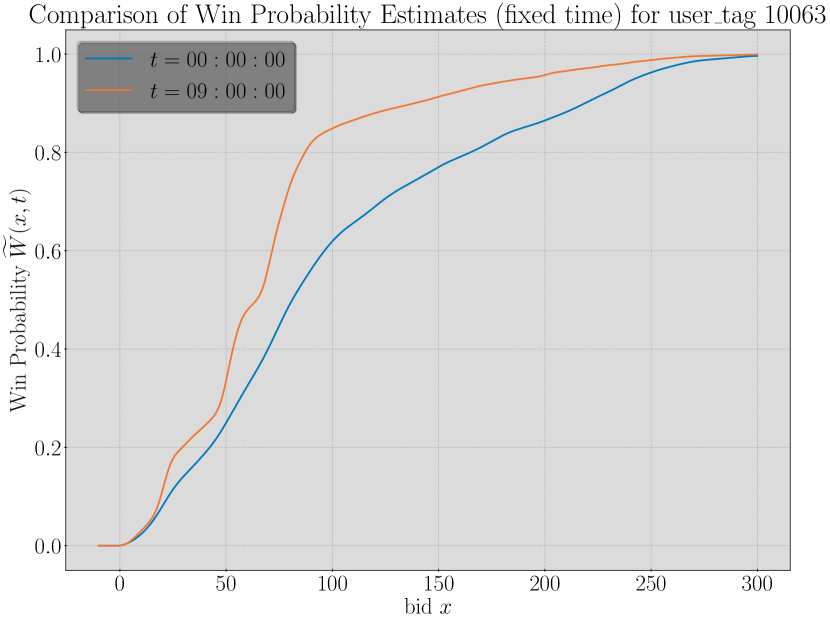
(b) Win Probability Estimates

Figure 1: Estimated Supply Rate Curves and Costs

Supply rate and win probability curves estimated from iPinYou data. $(a)$ Item arrival rates and the corresponding forecasts. The hatched region indicates an in-sample period with the remainder being out-of-sample. $(b)$ Estimates of the win probability function $\widetilde{W}(x,t)$ are obtained via Gaussian Kernel Density Estimates.

2.2 Problem Definition

Our goal is to find a bid path $x(t)\in\mathbb{R}^{N\times M}$ and allocation path $\gamma(t)\in[0,1]^{N\times M}$ which solves the following problem:

$$\underset{x,\gamma}{\text{minimize}} \sum_{i=1}^{N}\int_{0}^{T_{i}}\Bigl{[}\sum_{j\in\mathcal{A}_{i}}\gamma_{ij}(t)f_{j}(x_{ij}(t),t)\Bigr{]}\mathsf{d}t TP$$ ()

subject to $$\sum_{j\in\mathcal{A}_{i}}\int_{0}^{T_{i}}\gamma_{ij}(t)W_{j}(x_{ij}(t),t)\mathsf{d}t\geq C_{i}$$

$$\sum_{i\in\mathcal{B}_{j}}\gamma_{ij}(t)\leq 1,\gamma_{ij}(t)\geq 0,$$

where it is to be understood that constraints containing unqualified indices are to hold over their whole range. That is, $\gamma_{ij}(t)\geq 0$ is short for: $\forall(i,j)\in\mathcal{G}\ \forall t\in[0,T_{i}]\ \gamma_{ij}(t)\geq 0$. Additionally, functions $\gamma_{ij}(t),x_{ij}(t)$ etc. are treated as $0$ or undefined outside of $t\in[0,T_{i}]$. The notation

$$\mathcal{T}_{t}\overset{\Delta}{=}\{i\in[N]\ |\ t<T_{i}\}\\$$ (4)

indicating the contracts active up to time $t$ will be useful in keeping track of active contracts.

The variable $\gamma_{ij}(t)$, referred to as the allocation, parameterizes the proportion of items of type $j$ which will be bid on on behalf of contract $i$. Similarly, $x_{ij}(t)$ indicates the bid that should be submit for an item of type $j$ on behalf of contract $i$. Concretely, upon the arrival of an item of type $j$ at time $t$, the DSP bids on the item with probability $\Gamma_{j}(t)=\sum_{i\in\mathcal{B}_{j}}\gamma_{ij}(t)$, and if they have chosen to bid they do so on contract $i$ with probability $\gamma_{ij}(t)/\Gamma_{j}(t)$, and finally place the bid $x_{ij}(t)$ on the item. We have here allowed for the possibility of placing different bids depending upon which contract the item will be allocated towards, however, it will be shown in the sequel that this is never necessary and that Problem ($TP$) could have been written with bids $x_{j}(t)$ indexed only by $j$ and $t$, rather than the triple $i,j,t$.

We set the stage for our solution of Problem ($TP$) with some final conventions.

Definition 2.1 (Conventions).

We write $W_{j}^{-1}(x,t)$ for the inverse function of $x\mapsto W_{j}(x,t)$. The inverse is guaranteed to exist on the range of $W_{j}$ since the function is strictly monotone. Outside the range, the inverse is understood to be $+\infty$, i.e., $W_{j}^{-1}(s,t)=\infty$ if there is no $x\in\mathbb{R}$ such that $W_{j}(x,t)=s$. Typically, we will use $x$ for bids and $s$ for units of supply.

2.3 Convex Acquisition Costs

The key to understanding Problem ($TP$) is to consider acquisition cost functions:

$$\Lambda_{j}(s,t)\overset{\Delta}{=}f_{j}\circ W_{j}^{-1}(s,t)$$ (5)

which quantify, instantaneously at time $t$, the average cost of acquiring supply at the rate $s$.

In the second price case, the acquisition cost function is always convex. Indeed, this can be seen by a change of variables $y=W(u)$

$$\Lambda^{2nd}(s) =\mathbf{1}_{\mathbb{R}_{+}}(W^{-1}(s))\int_{0}^{W^{-1}(s)}u\mathsf{d}W(u)$$

$$=\mathbf{1}_{\{s\geq W(0)\}}\int_{W(0)}^{s}W^{-1}(y)\mathsf{d}y,$$

which is convex since its (one-sided) derivative on the domain is monotone non-decreasing. The interpretation of this result is that the marginal acquisition costs are increasing [26]. This is entirely natural for second price auctions since you pay the same amount for items that would be won by bids of $x$, whether or not you’re bidding exactly this amount, or something greater.

For the case of first price auctions, while total costs are necessarily always greater for greater bids, the marginal costs need not necessarily be increasing and therefore convexity does not always hold. In order to understand when it does, we need to discuss the idea of log-concavity. Recall that a function $W$ is log-concave if $\ln\circ W$ is concave and that any concave function is log-concave, but that the converse is false. The following notion of concavity, which includes both concavity and log-concavity, is utilized in our analysis.

Definition 2.2 ($\alpha$-concavity).

Define, for $\alpha\geq 0$, $x>0$ the function

$$\ell_{\alpha}(x)\overset{\Delta}{=}\int_{1}^{x}\frac{1}{t^{\alpha}}\mathsf{d}t=\left\{\begin{array}[]{lr}\ln x&\alpha=1\\ \frac{x^{1-\alpha}-1}{1-\alpha}&\text{otherwise}\end{array}\right.,$$

where in particular $\ell_{2}(x)=1-1/x$. We will say that a positive function $W:\mathbb{R}\rightarrow(0,\infty)$ is (strictly) $\alpha$-concave if $\ell_{\alpha}\circ W$ is (strictly) concave. In particular, $W$ is log-concave if $\alpha=1$ and concave if $\alpha=0$.

The following observation tells us that for any $\alpha>1$, $\alpha$-concavity is a weaker requirement than log-concavity, which is in turn weaker than concavity.

[restate, end, category=aux, no link to proof]proposition[Hierarchy of $\alpha$-concavity] For $0\leq\alpha<\beta$, if $W$ is $\alpha$-concave, then it is also $\beta$-concave. First we check that $\ell_{\beta}\circ\ell_{\alpha}^{-1}(x)$ is both monotone increasing and concave. This follows if the first derivative

$$\frac{\mathsf{d}}{\mathsf{d}x}\ell_{\beta}\circ\ell_{\alpha}^{-1}(x)=\frac{\ell_{\beta}^{\prime}\circ\ell_{\alpha}^{-1}(x)}{\ell_{\beta}^{\prime}\circ\ell_{\alpha}^{-1}(x)},$$

is positive and monotone non-increasing; which, since $\ell_{\alpha}^{-1}$ is itself monotone non-decreasing, follows if

$$\frac{\ell_{\beta}^{\prime}(x)}{\ell_{\alpha}^{\prime}(x)}$$

is both positive and monotone decreasing. Since $\ell_{\alpha}^{\prime}(x)=x^{-\alpha}$ this function is $x^{\alpha-\beta}$, which is positive on the domain $x>0$ and decreasing if $\alpha<\beta$.

Now, we check concavity of $\ell_{\beta}\circ W$ directly from the definition, for $t\in(0,1)$:

$$\ell_{\beta}\circ W(tx+(1-t)y) =\ell_{\beta}\circ\ell_{\alpha}^{-1}\circ\ell_{\alpha}\circ W(tx+(1-t)y)$$

$$\overset{(a)}{\geq}\ell_{\beta}\circ\ell_{\alpha}^{-1}\bigl{(}t\ell_{\alpha}\circ W(x)+(1-t)\ell_{\alpha}\circ W(y)\bigr{)}$$

$$\overset{(b)}{\geq}t\ell_{\beta}\circ\ell_{\alpha}\circ\ell_{\alpha}^{-1}\circ W(x)+(1-t)\ell_{\beta}\circ\ell_{\alpha}^{-1}\circ\ell_{\alpha}\circ W(y)$$

$$=t\ell_{\beta}\circ W(x)+(1-t)\ell_{\beta}\circ W(y),$$

where $(a)$ follows by the assumed concavity of $\ell_{\alpha}\circ W$ and the monotonicity of $\ell_{\beta}\circ\ell_{\alpha}^{-1}$ while $(b)$ from the concavity of $\ell_{\beta}\circ\ell_{\alpha}^{-1}$.

We can now characterize the conditions under which the cost of acquisition function $\Lambda_{j}(s,t)$ is convex in $s$ for first price auctions. As discussed above, a similar statement holds for the second price case, and doesn’t require the log-concavity assumption.

[end, restate, category=main, no link to proof]proposition[Convex Acquisition Costs – First Price Case] Suppose that a supply rate curve $W(x)$ is strictly $2$-concave. Then in a first price auction, the extended acquisition function

$$\Lambda^{1st}(s)\overset{\Delta}{=}\left\{\begin{array}[]{lr}\infty;&s>\bar{s}\\ 0;&s<W(0)\\ sW^{-1}(s);&\mathrm{otherwise}\end{array}\right.,$$ (6)

is a proper, lower semi-continuous, non-decreasing, and convex function on $\mathbb{R}$, which is strictly convex on $[W(0),\bar{s}]$. Moreover, the convex conjugate

$$\Lambda^{*}_{1st}(p)\overset{\Delta}{=}\underset{s\in\mathbb{R}}{\mathrm{sup}}\bigl{[}sp-\Lambda(s)\bigr{]},$$

is itself a proper, lower semi-continuous, non-decreasing, and convex function on $\mathbb{R}$, which satisfies $\Lambda^{*}_{1st}(p)=\infty$ for $p<0$, and if $\bar{s}<\infty$, then $\Lambda^{*}_{1st}(p)=p\bar{x}-\Lambda_{1st}(\bar{s})$ on $p>\bar{x}$. Since $f(x)=xW(x)\mathbf{1}_{\mathbb{R}_{+}}(x)$ we have, for $s\in\mathsf{ran}\ W$, $\Lambda(s)=sW^{-1}(s)$. On $s\leq W(0)$ we have $\Lambda(s)=0$, and on $s\in\{s|s>\bar{s}\}$ we have $\Lambda(s)=\infty$. Moreover, by Assumption 2.1, $W$ attains its supremum (when finite) and so $\Lambda$ is continuous at $\bar{s}$. Convexity will therefore follow if $\Lambda$ is convex on $\mathsf{int}\ \mathsf{ran}\ W$. To this end, we use the $2$-concavity of $W$ to see that $1-1/W(x)$ is concave on its domain and therefore that the inverse, $W^{-1}\bigl{(}1/(1-x)\bigr{)}$ is convex for the portion of $x\in(-\infty,1)$ which remains in the range of $W$. It is fairly well known that for a convex function $f$, the function

$$(cx+d)f\bigl{(}\frac{ax+b}{cx+d}\bigr{)}$$

is convex on $cx+d>0$ (see e.g. [5, Ex. 3.20]. Therefore, by setting $a=c=1$, $b=-1$ and $d=0$ we obtain convexity of

$$(cs+d)W^{-1}\Bigl{(}\frac{cs+d}{(c-a)s+(d-b)}\Bigr{)}=sW^{-1}\bigl{(}s\bigr{)}$$

which is the function $\Lambda(s)$.

In consideration of the conjugate, it is evident that since $\Lambda(s)\geq 0$ we have $\Lambda^{*}(p)=\infty$ for $p<0$ (take $s\rightarrow-\infty$). For $p>\bar{x}$, if $\bar{s}<\infty$, then since $s<\bar{s}\implies W^{-1}(s)<\bar{x}$ and $\Lambda(\bar{s}+)=\infty$ we see that $sp-\Lambda(s)$ is maximized at $s=\bar{s}$. That $\Lambda^{*}(p)$ is non-decreasing follows since for $p\leq q$ we have $sp-\Lambda(s)\leq sq-\Lambda(s)$ on $s\geq 0$. Finally, that $\Lambda^{*}(p)$ is proper, lower semi-continuous, and convex is a statement of the Fenchel-Moreau Theorem (see e.g., [9, sec 4.2]).

2.4 Optimal Bidding in Continuous Time

As long as the acquisition cost functions are convex, we can equivalently reformulate Problem ($TP$) as the following continuous time convex optimization problem. This reformulation is not trivial and makes use of the existence of a campaign-independent optimal bid $x_{ij}(t)=x_{j}(t)$, the existence of which is established by using the convexity of $\Lambda$.

[end, restate, category=main, no link to proof]proposition[Continuous Primal Problem] In a first or second price auction, suppose that for each $j\in[M]$ and $t\in[0,T^{j}]$, the acquisition cost curve $\Lambda_{j}(x,t)$ is convex in $x$. Then, Problem ($TP$) can be reformulated as

$$\underset{s,r}{\mathrm{minimize}} \sum_{j=1}^{M}\int_{0}^{T^{j}}\Lambda_{j}(s_{j}(t),t)\mathsf{d}t P$$ ()

$$\mathrm{subject\;to} \sum_{j\in\mathcal{A}_{i}}\int_{0}^{T_{i}}r_{ij}(t)\mathsf{d}t\geq C_{i}$$

$$\sum_{i\in\mathcal{B}_{j}}r_{ij}(t)=s_{j}(t)$$

$$r_{ij}(t)\geq 0.$$

If a solution exists, then a solution to the original problem ($TP$) is obtained via $x_{ij}(t)=W_{j}^{-1}(s_{j}(t),t)$ for each $i\in\mathcal{B}_{j}$ and $\gamma_{ij}(t)=r_{ij}(t)/s_{j}(t)$. Moreover, Problem ($P$) is convex. First, we establish that whenever a solution exists, there is also a solution with the property that $x_{ij}(t)=x_{j}(t)$ and where $\sum_{i\in\mathcal{B}_{j}}\gamma_{ij}(t)\in\{0,1\}$. To this end, suppose $(x,\gamma)$ is a solution of Problem ($TP$), and with total cost $J$. Let $(\tilde{x},\tilde{\gamma})$ be another bid and allocation pair with total cost $\tilde{J}$ defined by

$$\tilde{x}_{j}(t) \overset{\Delta}{=}W_{j}^{-1}\Bigl{(}\sum_{i\in\mathcal{B}_{j}}\gamma_{ij}(t)W_{j}(x_{ij}(t),t),t\Bigr{)},$$

$$\tilde{\gamma}_{ij}(t) \overset{\Delta}{=}\frac{\gamma_{ij}(t)W_{j}(x_{ij}(t),t)}{\sum_{u\in\mathcal{B}_{j}}\gamma_{uj}(t)W_{j}(x_{uj}(t),t)},$$

where $0/0\overset{\Delta}{=}0$ in the definition of $\tilde{\gamma}$. We proceed to show that $(\tilde{x},\tilde{\gamma})$ is also a solution and we note that the definition of $\tilde{\gamma}$ satisfies $\forall t<T^{j}\;\sum_{i\in\mathcal{B}_{j}}\tilde{\gamma}_{ij}(t)\in\{0,1\}$.

It is clear that the pair $\tilde{x},\tilde{\gamma}(t)$ is feasible by construction. Indeed, $\tilde{\gamma}_{ij}(t)\geq 0$ and $\sum_{i\in\mathcal{B}_{j}}\tilde{\gamma}_{ij}(t)\leq 1$ by definition. Moreover, we have

$$\sum_{j\in\mathcal{A}_{i}}\tilde{\gamma}_{ij}(t)W_{j}(\tilde{x}_{j}(t),t) =\sum_{j\in\mathcal{A}_{i}}\Bigl{[}\frac{\gamma_{ij}(t)W_{j}(x_{ij}(t),t)\sum_{v\in\mathcal{B}_{j}}\gamma_{vj}(t)W_{v}(x_{vj}(t),t)}{\sum_{u\in\mathcal{B}_{j}}\gamma_{uj}(t)W_{j}(x_{uj}(t),t)}\Bigr{]}$$

$$=\sum_{j\in\mathcal{A}_{i}}\gamma_{ij}(t)W_{j}(x_{ij}(t),t),$$

which when integrated from $0$ to $T_{i}$ meets or exceeds $C_{i}$ since $(x,\gamma)$ is assumed to be a solution.

The cost of $(\tilde{x},\tilde{\gamma})$, instantaneously at time $t$, then satisfies $\tilde{J}=J$ since $J$ is the minimal cost and

$$\tilde{J} \overset{\Delta}{=}\int_{0}^{T}\Bigl{[}\sum_{i=1}^{N}\sum_{j\in\mathcal{A}_{i}}\tilde{\gamma}_{ij}(t)f_{j}(\tilde{x}_{j}(t))\Bigr{]}\mathsf{d}t$$

$$\overset{(a)}{=}\int_{0}^{T}\Bigl{[}\sum_{i=1}^{N}\sum_{j\in\mathcal{A}_{i}}\tilde{\gamma}_{ij}(t)\Lambda_{j}\Bigl{(}\sum_{u\in\mathcal{B}_{j}}\gamma_{uj}(t)W_{j}(x_{uj}(t),t),t\Bigr{)}\Bigr{]}\mathsf{d}t$$

$$\overset{(b)}{\leq}\int_{0}^{T}\Bigl{[}\sum_{i=1}^{N}\sum_{j\in\mathcal{A}_{i}}\tilde{\gamma}_{ij}(t)\sum_{u\in\mathcal{B}_{j}}\gamma_{uj}(t)\Lambda_{j}(W_{j}(x_{uj}(t),t),t)\Bigr{]}\mathsf{d}t$$

$$\overset{(c)}{=}\int_{0}^{T}\Bigl{[}\sum_{j=1}^{M}\sum_{u\in\mathcal{B}_{j}}\gamma_{uj}(t)f_{j}(x_{uj}(t),t)\sum_{i\in\mathcal{B}_{j}}\tilde{\gamma}_{ij}(t)\Bigr{]}\mathsf{d}t=J$$

where $(a)$ is just the definition of $\Lambda_{j}=f_{j}\circ W_{j}^{-1}$ (see Section 2.3), $(b)$ follows by the convexity of $\Lambda_{j}$ and that $\Lambda_{j}(0)=0$ (since $\gamma_{ij}$ need not necessarily sum to $1$), and $(c)$ follows again by $\Lambda_{j}=f_{j}\circ W_{j}^{-1}$ and then by swapping the order of summation using $i\in\mathcal{B}_{j}\iff j\in\mathcal{A}_{i}$.

We can now recall the original problem ($TP$), and apply the preceding results to eliminate the dependence of the bid on $i$, since if a solution exists it can be assumed to have the property $x_{ij}(t)=x_{j}(t)$:

$$\underset{x,\gamma}{\text{minimize}} \sum_{i=1}^{N}\int_{0}^{T_{i}}\Bigl{[}\sum_{j\in\mathcal{A}_{i}}\gamma_{ij}(t)f_{j}(x_{j}(t),t)\Bigr{]}\mathsf{d}t$$

subject to $$\sum_{j\in\mathcal{A}_{i}}\int_{0}^{T_{i}}\gamma_{ij}(t)W_{j}(x_{j}(t),t)\mathsf{d}t\geq C_{i}$$

$$\sum_{i\in\mathcal{B}_{j}}\gamma_{ij}(t)\leq 1,\gamma_{ij}(t)\geq 0,$$

Due to the bids’ independence of $i$, we can rearrange the objective by swapping the order of summation:

$$\sum_{i=1}^{N}\int_{0}^{T_{i}}\Bigl{[}\sum_{j\in\mathcal{A}_{i}}\gamma_{ij}(t)f_{j}(x_{j}(t),t)\Bigr{]}\mathsf{d}t=\sum_{j=1}^{M}\int_{0}^{T^{j}}\Bigl{[}f_{j}(x_{j}(t),t)\sum_{i\in\mathcal{B}_{j}}\gamma_{ij}(t)\Bigr{]}\mathsf{d}t,$$ (7)

which, after making the substitution $s_{j}(t)=W_{j}(x_{j}(t),t)$, results in

$$\underset{s,\gamma}{\text{minimize}} \sum_{j=1}^{M}\int_{0}^{T^{j}}\Bigl{[}\Lambda_{j}(s_{j}(t),t)\sum_{i\in\mathcal{B}_{j}}\gamma_{ij}(t)\Bigr{]}\mathsf{d}t$$ (8)

subject to $$\int_{0}^{T_{i}}\sum_{j\in\mathcal{A}_{i}}\gamma_{ij}(t)s_{j}(t)\geq C_{i}$$

$$\sum_{i\in\mathcal{B}_{j}\cap\mathcal{T}_{t}}\gamma_{ij}(t)\leq 1$$

$$\gamma_{ij}(t)\geq 0,s_{j}(t)\geq 0.$$

Now, since any optimal solution can be assumed to be such that $\sum_{i\in\mathcal{B}_{j}}\gamma_{ij}(t)\in\{0,1\}$ and since $\Lambda_{j}(0,t)=0$, there is no loss of generality in adding the constraint $\sum_{i\in\mathcal{B}_{j}}\gamma_{ij}(t)=1$ and eliminating this term from the objective. Finally, making the substitution $r_{ij}(t)=\gamma_{ij}(t)s_{j}(t)$ results in the formulation of Problem ($P$).

Remark 2.6 (Connection to Transportation-Production Problems).

This result demonstrates that Problem ($TP$) can be reformulated as an instance of a (convex) Transportation-Production problem (see [26, 35]) in continuous time (hence the label ($TP$)), which is in turn an example of a monotropic program [34, 4]. To see this connection, one can think of $i$ as the “consumption nodes”, $j$ as the “production nodes”, the graph $\mathcal{G}$ (defined through the sets $\mathcal{A}_{i},\mathcal{B}_{j}$) as defining the transportation network, and the functions $f_{j},W_{j},\Lambda_{j}$ as characterizing the costs of production.

In order for a solution to exist, it is necessary only that an adequate amount of supply is available to fulfill each contract before its deadline. In the context of internet advertising, this is not unreasonable, and a coarse sufficient condition is $W(x)\rightarrow\infty$ as $x\rightarrow\infty$. As in the case of finite optimization problems, strong duality obtains if there is a strictly feasible point.

Assumption 2.2 (Adequate Supply).

We suppose that $\exists x\in\mathbb{R}^{M}$ such that the following linear feasibility problem has a strictly feasible point (i.e., a Slater point)

$$\mathrm{find}\quad\gamma_{ijk}$$ (9)

$$\mathrm{such\ that} \sum_{k:T_{k}\leq T_{i}}\sum_{j\in\mathcal{A}_{i}}\gamma_{ijk}\int_{T_{k-1}}^{T_{k}}W_{j}(x_{j},t)\mathsf{d}t>C_{i}$$

$$\sum_{i\in\mathcal{B}_{j}}\gamma_{ijk}\leq 1,\gamma_{ijk}\geq 0.$$

That is, there exists a large enough constant bid such that an adequate amount of supply is attained.

Remark 2.7.

A simpler sufficient condition (appearing also in [26]) is to suppose that each curve has an adequate amount of supply to fulfill all the contracts to which it is assigned:

$$\forall j\in[M]\ \exists x\in\mathbb{R}:\ \int_{0}^{\tau_{j}}W_{j}(x,t)\mathsf{d}t>\sum_{i\in\mathcal{B}_{j}}C_{i},$$

where $\tau_{j}=\text{min}\{T_{i}\ |\ i\in\mathcal{B}_{j}\}$. Finally, this condition is clearly satisfied under the simple condition that if for each $j,t$ we have $W_{j}(x,t)\rightarrow\infty$ as $x\rightarrow\infty$.

[end, restate, category=main, no link to proof]proposition[Duality] A Dual of ($P$) can be formulated as

$$\underset{\rho,\mu}{\mathrm{maximize}} -\sum_{j=1}^{M}\sum_{k:T_{k}\leq T^{j}}\int_{T_{k-1}}^{T_{k}}\Lambda_{j}^{*}(\mu_{jk},t)\mathsf{d}t+\sum_{i=1}^{N}\rho_{i}C_{i} D$$ ()

$$\mathrm{subject\;to} \mu_{jk}\geq\rho_{i}\ \forall i\in\mathcal{B}_{j}\cap\mathcal{T}_{T_{k}}$$

$$\rho_{i}\geq 0,$$

which is a finite convex problem. Problem ($D$) is dual to Problem ($P$) in the sense that if $D^{\star}$ and $P^{\star}$ are their respective values (possibly $\infty$ or $-\infty$), then $D^{\star}\leq P^{\star}$.

Finally, under Assumption 2.2 there exists a solution $(s,r)\in L_{2}(\mathbb{R})^{M}\times L_{2}(\mathbb{R})^{N\times M}$ to Problem ($P$) and a solution $(\rho,\mu)\in\mathbb{R}^{N}\times\mathbb{R}^{M}$ to Problem ($D$) and $-\infty<D^{\star}=P^{\star}<\infty$.

The first part of the theorem is a simple statement of facts from convex analysis, and the strong duality result is based on Lagrange multiplier theory for real valued functions in a reflexive Banach space. In particular, we establish the existence of a solution to Problem ($P$) (in $L_{2}$) under Assumption 2.2 via the direct method (see e.g., [9, thm. 5.51]) and strong duality via the methods of [9, Ch. 9].

Consider a Lagrangian of Problem ($P$):

$$\mathcal{L}(s,r,\rho,\mu) =\sum_{j=1}^{M}\int_{0}^{T^{j}}\Lambda_{j}(s_{j}(t),t)\mathsf{d}t+\sum_{i=1}^{N}\rho_{i}\Bigl{[}C_{i}-\sum_{j\in\mathcal{A}_{i}}\int_{0}^{T_{i}}r_{ij}(t)\mathsf{d}t\Bigr{]}$$ (10)

$$\quad+\sum_{j=1}^{M}\int_{0}^{T^{j}}\mu_{j}(t)\Bigl{[}\sum_{i\in\mathcal{B}_{j}}r_{ij}(t)-s_{j}(t)\Bigr{]}\mathsf{d}t$$

with the problem domain $S=\text{dom }\mathcal{L}$ restricted to a convex subset of $L_{2}$:

$$S\overset{\Delta}{=}\mathcal{P}\times\mathcal{D}\overset{\Delta}{=}\{(r,s),(\rho,\mu)\ |\ r_{ij}(t)\geq 0,\rho_{i}\geq 0,\mu_{j}(t)\geq 0\}.$$

It is well known that the primal problem ($P$) can be posed as finding $s,r$ which attains the infima:

$$\underset{s,r\in\mathcal{P}}{\text{inf}}\ \underset{\rho,\mu\in\mathcal{D}}{\text{sup}}\ \mathcal{L},$$

since the suprema is $\infty$ whenever the constraints of ($P$) are not met. Moreover, it is a general theorem (the max-min inequality) that

$$D^{\star}\overset{\Delta}{=}\underset{\rho,\mu\in\mathcal{D}}{\text{sup}}\ \underset{s,r\in\mathcal{P}}{\text{inf}}\ \mathcal{L}\leq\underset{s,r\in\mathcal{P}}{\text{inf}}\ \underset{\rho,\mu\in\mathcal{D}}{\text{sup}}\ \mathcal{L}\overset{\Delta}{=}P^{\star}.$$

We proceed to show that finding $\rho,\mu$ to maximize $\inf_{s,r\in\mathcal{P}}\mathcal{L}$ is equivalent to ($D$). Consider first the $r$ variable, we have:

$$\underset{r\geq 0}{\text{inf}}\ \sum_{i=1}^{N}\sum_{j\in\mathcal{A}_{i}}\int_{0}^{T_{i}}\bigl{(}\mu_{j}(t)-\rho_{i}\bigr{)}r_{ij}(t)\mathsf{d}t,$$

which is $-\infty$ unless $\mu_{j}(t)\geq\rho_{i}$ for $i\in\mathcal{B}_{j}$. Next, examine $\text{inf}_{s}\ \mathcal{L}$:

$$\underset{s}{\text{inf}}\ \sum_{j=0}^{M}\int_{0}^{T^{j}}\Bigl{[}\Lambda_{j}(s_{j}(t),t)\mathsf{d}t-\mu_{j}(t)s_{j}(t)\Bigr{]},$$

which can be computed point-wise (it will be clear that the resulting function is in $L_{2}$) as

$$\underset{s}{\text{inf}}\ \bigl{[}\Lambda_{j}(s_{j},t)-\mu_{j}s_{j}\bigr{]} =-\underset{s}{\text{sup}}\ \bigl{[}\mu_{j}s_{j}-\Lambda_{j}(s_{j},t)\bigr{]}$$

$$=-\Lambda_{j}^{*}(\mu_{j},t),$$

the negative of the conjugate of $s\mapsto\Lambda_{j}(s,t)$ (see Proposition 2.2). Combining these calculations together results in the following problem:

$$\underset{\rho,\mu}{\mathrm{maximize}} -\sum_{j=1}^{M}\int_{0}^{T^{j}}\Lambda_{j}^{*}(\mu_{j}(t),t)\mathsf{d}t+\sum_{i=1}^{N}\rho_{i}C_{i}$$ (11)

$$\mathrm{subject\;to} \mu_{j}(t)\geq\rho_{i}\ \forall i\in\mathcal{B}_{j}\cap\mathcal{T}_{t}$$

$$\rho_{i}\geq 0.$$

Suppose that $\rho_{i}$ is optimal for this problem. Then, since $\Lambda^{*}$ is monotone increasing, the optimal $\mu_{j}(t)$ is the smallest possible, which implies we can take $\mu_{j}(t)$ to be piecewise constant between contract deadlines (any deviation over a positive measure interval increases the cost, and any deviation over a measure zero set doesn’t change the cost). Denote by $\mu_{jk}$ the value taken by the optimal $\mu_{j}(t)$ over $[T_{k-1},T_{k}]$ for $T_{k}\leq T^{j}$ to obtain Problem ($D$). Indeed, it can be seen that $\mu_{jk}=\underset{i\in\mathcal{B}_{j}\cap\mathcal{T}_{T_{k}}}{\text{max}}\ \rho_{i}$.

Finally, we show the existence of solutions to both ($P$) and ($D$), as well as the equality of their values, under the adequate supply assumption 2.2.

Under Assumption 2.2 the $\mathbb{R}$-valued function on $L_{2}(\mathbb{R})^{M}\times L_{2}(\mathbb{R})^{N\times M}$ defined by $(s,r)\mapsto\underset{\rho,\mu}{\text{sup}}\ \mathcal{L}(s,r,\rho,\mu)$ is a proper, convex, and l.s.c. function. That this function is proper follows from the assumption since there is at least one feasible point, the convexity follows since suprema over families of affine functions are convex, and lower semi-continuity follows since this property is preserved through the suprema. Naturally, the restriction of $S$ to the primal variables $(s,r)$ remains closed and convex.

Now, by the basic properties of $W_{j}$ (Assumption 2.1) $\Lambda_{j}(s)$ is positively-coercive (i.e. $\Lambda_{j}(s)\rightarrow\infty$ as $s\rightarrow\infty$); this property is thus inherited by the function $s\mapsto\underset{\rho,\mu}{\text{sup}}\ \mathcal{L}(s,r,\rho,\mu).$ Indeed, by the construction of $\mathcal{L}$ the function $r\mapsto\underset{\rho,\mu}{\text{sup}}\ \mathcal{L}(s,r,\rho,\mu)$ must be positively-coercive as well since if $\sum_{i\in\mathcal{B}_{j}}r_{ij}(t)\neq s_{j}(t)$ then ${\text{sup}}\ \mathcal{L}(s,r,\rho,\mu)=\infty$. Then, keeping in mind that $(s,r)\in S\implies s,r\geq 0$, this is enough to satisfy the growth condition required by [9, thm. 5.51 (c)] and establishes the existence of a solution to $\underset{s,r}{\text{inf}}\ \underset{\rho,\mu}{\text{sup}}\ \mathcal{L}$ and therefore to $(P)$.

The statement of strong duality now follows from combining [9, thm. 9.8] and [9, thm. 9.13] with Assumption 2.2.

Finally, the optimal bid path $x(t)$ for Problem ($TP$) can be reconstructed from solutions to ($D$) and is, in fact, fully characterized by the finite vector $\rho\in\mathbb{R}^{N}$, which we designate as the vector of pseudo-bids.

[normal]example[Pseudo Bids] Suppose that $\mu_{jk},\rho_{i}$ are optimal dual multipliers for the Problem ($D$) and consider the $s$-dependent portion of the Lagrangian:

$$L(s)=\sum_{j=1}^{M}\int_{0}^{T^{j}}\Bigl{[}\Lambda_{j}(s_{j}(t),t)-\mu_{j}(t)s_{j}(t)\Bigr{]}\mathsf{d}t,$$

where $\mu_{j}(t)=\mu_{jk}$ for $t\in[T_{k-1},T_{k})$ is piecewise constant.

Minimizing this function over $s_{j}(t)$ leads to an optimal supply path as a function of $\mu_{j}(t)$. Since the above function is convex, we know that the optimum is attained at $s_{j}(t)$ such that the pointwise selection holds:

$$\mu_{j}(t)\in\partial\Lambda_{j}(s_{j}(t),t),$$ (12)

where $\partial$ indicates the subdifferential and is with respect to the first argument. Therefore, since $\mu_{j}(t)=\underset{i\in\mathcal{B}_{j}\cap\mathcal{T}_{t}}{\text{max}}\ \rho_{i}$, the entire optimal supply path $s(t)$, and therefore the entire optimal bid path $x(t)$, is fully determined by the finite vector $\rho\in\mathbb{R}^{N}$ through Equation (12). For this reason, we refer to $\rho$ as the vector of pseudo bids.

2.5 Connections Between First and Second Price Auctions

It will be seen in Section 3.2 that, empirically, the optimal solution calculated for the second price auction also provides very good bid and allocation paths for the first price auction. From Example 2.7, we know that the optimal solutions cannot be exactly the same (except perhaps in some coincidental cases), but we explain the empirical similarity by illuminating the close connection between the first and second price cases in the following proposition.

[restate, end, category=aux, no link to proof]proposition[Connection Between First and Second Price Case] Under Assumption 2.2, and whenever the acquisition cost curves are convex, the Problem ($TP$) for a second price auction is equivalent to solving

$$\underset{x,\gamma,\rho}{\mathrm{minimize}} \sum_{j=1}^{M}\int_{0}^{T^{j}}x_{j}(t)W_{j}(x_{j}(t),t)\mathsf{d}t-\sum_{i=1}^{N}\rho_{i}C_{i}$$ (13)

$$\mathrm{subject\ to} \sum_{j\in\mathcal{A}_{i}}\int_{0}^{T_{i}}\gamma_{ij}(t)W_{j}(x_{j}(t),t)\geq C_{i}$$

$$\sum_{i\in\mathcal{B}_{j}}\gamma_{ij}(t)=1,\gamma_{ij}(t)\geq 0,\rho_{i}\geq 0$$

$$x_{j}(t)\geq\rho_{i}\ \forall i\in\mathcal{B}_{j}\cap\mathcal{T}_{t}.$$

The objective function involves $x_{j}(t)W_{j}(x_{j}(t),t)$, which is the cost associated with a first price auction. We first examine the conjugate function for the second price acquisition function. We have

$$\Lambda_{2nd}(s)\overset{\Delta}{=}\left\{\begin{array}[]{lr}\infty;&s>\bar{s}\\ 0;&s<W(0)\\ \int_{W(0)}^{s}W^{-1}(y)\mathsf{d}y;&\mathrm{otherwise}\end{array}\right..$$ (14)

We can find the conjugate on a segment of $\mathbb{R}$ by differentiation:

$$\Lambda^{*}_{2nd}(\mu)=\underset{s}{\text{sup}}\bigl{[}s\mu-\Lambda(s)\bigr{]},$$

leading to the supremum being attained at $s=W(\mu)$ as long as $\mu\in[0,\bar{x}]$ (in which case the derivative is indeed $W^{-1}(s)$). We already know from Proposition 2.2 that when $\mu<0$ we have $\Lambda^{*}(\mu)=\infty$ and if $\bar{s}<\infty$ and $\mu>\bar{x}$, then $\Lambda^{*}(\mu)=\bar{s}\mu-\Lambda(\bar{s})$.

Therefore, since $\Lambda(W(\mu))=f(\mu)$ by definition, we have

$$\Lambda^{*}_{2nd}(\mu)=\left\{\begin{array}[]{lr}\infty;&\mu<0\\ \mu\bar{s}-\Lambda_{2nd}(\bar{s});&\mu>\bar{x}\\ \mu W(\mu)-f_{2nd}(\mu);&\text{otherwise}\end{array}\right..$$ (15)

Given a dual solution $\mu,\rho$ of Problem ($D$), which attains the primal problem’s value by strong duality Proposition 2.7, we see from the above calculations that the maximizing argument for $\Lambda^{*}$ is just $s=W(\mu)$, therefore it must be the case that the optimal bid is the optimal multiplier $x_{j}(t)=\mu_{jk}$ on $t\in[T_{k-1},T_{k})$, which recovers the result of Example 2.7 that for the second price auction there exists an optimal piecewise constant bid.

Using this fact, and writing the dual as a minimization problem by negating its objective, we can consider the problem of simultaneously solving the dual ($D$) and the original Problem ($TP$)

$$\underset{x,\gamma,\rho}{\text{minimize}} \sum_{j=1}^{M}\int_{0}^{T^{j}}\bigl{[}f_{j}^{2nd}(x_{j}(t),t)+\Lambda_{j}^{*}(x_{j}(t),t)\bigr{]}\mathsf{d}t-\sum_{i=1}^{N}\rho_{i}C_{i}$$ (16)

subject to $$\sum_{j\in\mathcal{A}_{i}}\int_{0}^{T_{i}}\gamma_{ij}(t)W_{j}(x_{j}(t),t)\geq C_{i}$$

$$\sum_{i\in\mathcal{B}_{j}}\gamma_{ij}(t)=1,\gamma_{ij}(t)\geq 0,\rho_{i}\geq 0$$

$$x_{j}(t)\geq\rho_{i}\ \forall i\in\mathcal{B}_{j}\cap\mathcal{T}_{t},$$

where we have again applied the fact that there exists a solution such that $x_{ij}(t)=x_{j}(t)$ for every $i\in\mathcal{B}_{j}$ and where $\sum_{i\in\mathcal{B}_{j}}\gamma_{ij}(t)=1$ (see the proof of 2.4).

If we can show that the optimal dual multipliers satisfy $\mu_{jk}\leq\bar{x}_{j}$, then using the fact that $x_{j}(t)=\mu_{jk}$ for $t\in[T_{k-1},T_{k})$ and the expression for $\Lambda^{*}$ we have the result, since the $f_{j}^{2nd}$ terms cancel.

To this end, recognize that since $\mu_{jk}=\underset{i\in\mathcal{B}_{j}\cap\mathcal{T}_{T_{k}}}{\text{max}}\ \rho_{i}$, we must have $\mu_{jk}\leq\bar{x}_{j}$ unless there is some $\rho_{i}>\bar{x}_{j}$. We suppose by way of contradiction that $\rho_{i}>\bar{x}_{j}$. Consider the portion of the objective of ($D$) related to contract $i$ (where $\Lambda=\Lambda_{2nd}$):

$$-\sum_{j\in\mathcal{A}_{i}}\sum_{k:T_{k}\leq T_{i}}\int_{T_{k-1}}^{T_{k}}\Lambda_{j}^{*}(\mu_{jk},t)\mathsf{d}t+\rho_{i}C_{i} \overset{(a)}{\leq}\rho_{i}C_{i}-\sum_{j\in\mathcal{A}_{i}}\int_{0}^{T_{i}}\Lambda_{j}^{*}(\rho_{i},t)\mathsf{d}t$$

$$\overset{(b)}{=}\rho_{i}C_{i}-\sum_{j\in\mathcal{A}_{i}}\int_{0}^{T_{i}}(\rho_{i}\bar{s}_{j}(t)-\Lambda_{j}(\bar{s}_{j}(t),t))\mathsf{d}t$$

$$=\sum_{j\in\mathcal{A}_{i}}\int_{0}^{T_{i}}\Lambda_{j}(\bar{s}_{j},t)\mathsf{d}t+\rho_{i}\Bigl{[}C_{i}-\int_{0}^{T_{i}}\bar{s}_{j}(t)\mathsf{d}t\Bigr{]}$$

$$\overset{(c)}{<}\sum_{j\in\mathcal{A}_{i}}\int_{0}^{T_{i}}f_{j}(\bar{x}_{j}(t),t)\mathsf{d}t$$

where $(a)$ follows from $\mu_{jk}\geq\rho_{i}$ since $\Lambda^{*}$ is non-decreasing, $(b)$ from Equation (15) since $\rho_{i}>\bar{x}_{j}$, and $(c)$ from $\rho_{i}\geq 0$ combined with Assumption 2.2 which ensures the bracketed term is negative. The final expression is the cost attained by bidding $\bar{x}_{j}(t)$ so by strong duality $\rho_{i}>\bar{x}_{j}$ must not have been optimal (recall that in the dual we are maximizing). Therefore, $\mu_{jk}\leq\bar{x}_{j}$, which completes the proof.

Returning to Example 2.7, we can make a further explicit comparison between the two cases.

[normal]example[Pseudo Bids (continued)] For the purpose of illustration, let us temporarily assume that our supply rate curves are smooth in the bid $x$, and that the optimal solutions satisfy $s_{j}(t)\in(W_{j}(0,t),\bar{s}_{j}(t))$ (i.e., do not reach the extremes of available supply) so that we have the simple expressions $\Lambda^{2nd}_{j}(s,t)=\int_{W_{j}(0,t)}^{s}W_{j}^{-1}(y,t)\mathsf{d}y$ and $\Lambda^{1st}_{j}(s)=sW_{j}^{-1}(s,t)$. For the first price case, let us define a function $g_{j}$, where ^′ denotes differentiation with respect to $x$:

$$g_{j}(x,t)\overset{\Delta}{=}\frac{f_{j,1st}^{\prime}(x,t)}{W_{j}^{\prime}(x,t)}=x+\frac{W_{j}(x,t)}{W_{j}^{\prime}(x,t)}.$$

We can then solve Equation 12 for the optimal bid in terms of $\mu_{j}$, which in the first price case, can be written in terms of $g$: $\Lambda^{\prime-1}_{j}(x,t)=W_{j}\circ g_{j}^{-1}(x,t)$. The second price case is much simpler, and we have $\Lambda^{\prime}_{2nd}(x,t)=W^{-1}(s,t)$. That is, the analogous ’$g$’ function for the second price case is the identity.

Now, in each case we map the desired supply $s$ into the required bid $x$ through $x_{j}(t)=W_{j}^{-1}(s_{j}(t),t)$ and find that the optimal bids for each case are

$$x_{j}(t)=\left\{\begin{array}[]{lr}\mu_{j}^{2nd}(t)&\text{Second Price}\\ g_{j}^{-1}(\mu_{j}^{1st}(t),t)&\text{First Price},\end{array}\right.$$ (17)

where $\mu_{j}^{2nd}(t)$ is the dual multipliers associated to Problem ($D$) with second price cost function and $\mu_{j}^{1st}$ are multipliers of the same problem but with the first price cost function; that is, $\mu_{j}^{1st}\neq\mu_{j}^{2nd}$ in general. It is important to recognize that $\mu(t)$ is a piecewise constant function which is fully determined by $\rho\in\mathbb{R}^{N}$. The implication being that in each case, the entire time-dependent optimal bid path is fully characterized by the finite vector $\rho$ associated to the dual problem ($D$).

The upshot of these calculations is that in the second price case, the optimal bid path is constant between contract deadlines, whereas in the first price case the pseudo bids need to be mapped through the function $g^{-1}$. The intuition for this fact is that in a second price case you are “protected” from overpaying (since you only pay the second highest bid) whereas in the first price case you need to adapt the bids to your belief about the prevailing prices.

If the supply rate curves are time-independent (i.e. $W(x,t)=W(x)$), then the function $g_{j}^{-1}$ is time-independent as well. It may be conjectured that in this case the optimal bids would coincide, i.e., that $\mu_{j}^{2nd}(t)=g_{j}^{-1}(\mu_{j}^{1st}(t))$. Experimental evidence shows that this does not seem to be the case in general.

3 Computational Methods and Simulations

In this section we review computational methods useful for the implementation of our theory (Section 3.1); carry out a Monte Carlo simulation lending evidence to the similarity between the first and second price case, as suggested by Proposition 2.5 (Section 3.2); and finally provide basic results on practical methods for adapting to a stochastic environment (Section 3.3).

3.1 Computing and Implementing Optimal Bids

To summarize the developments so far, the solution to the optimal bidding and allocation problem ($TP$) consists of a bid path $x(t)$ and allocation path $\gamma(t)$. The function $\gamma_{ij}(t)$ indicates that if an item of type $j$ is won at auction at time $t$, then it should be allocated towards contract $i$ with probability $\gamma_{ij}(t)$. Therefore, upon the arrival of an item of type $j$, the bidder should sample a random index $\hat{i}\in\mathcal{B}_{j}$ from a categorical distribution with $\mathbb{P}\{\hat{i}=i\}=\gamma_{ij}(t)$. Then, the function $x_{\hat{i}j}(t)$ indicates the nominal bid which should be submit to the auction house (the actual bid being $\mathcal{N}(x_{\hat{i}j}(t),\sigma^{2})$ if randomization is used). Finally, if the item is won, it should be allocated to contract $\hat{i}$.

The Problem ($TP$) is, as written, not tractable. However, Proposition 2.4 tells us that the solution $s(t),r(t)$ to the convex problem ($P$) can be used to obtain the optimal bid and allocation through

$$x_{ij}(t) =W_{j}^{-1}(s_{j}(t),t),$$

$$\gamma_{ij}(t) =r_{ij}(t)/s_{j}(t),$$

where it is to be understood that $x_{ij}(t)=\gamma_{ij}(t)=0$ for any $j\not\in\mathcal{A}_{i}$ or $t>T_{i}$, and that any $0/0$ encountered in the construction of $\gamma_{ij}(t)$ is to be taken as $0$. Moreover, this formula tells us that we actually need to keep track of only $M$ bidding functions, $x_{j}(t)$, since there is an optimal solution such that $x_{ij}(t)=x_{i^{\prime}j}(t)$ for each $i,i^{\prime}\in\mathcal{B}_{j}$.

Problem ($P$) is still an infinite dimensional problem, and thus remains intractable as written. A solution could be obtained by first solving the dual ($D$) (which is finite, but requires integration), substituting the resulting pseudo-bids (through $g^{-1}$, see Example 2.5) into the original problem ($TP$) and solving the resulting linear program to obtain $\gamma(t)$. However, we have found that directly discretizing the primal problem and solving the resulting convex program tends to be faster and with limited degradation in accuracy. Moreover, solving the primal directly results in both the optimal bids and the optimal allocations simultaneously.

Therefore, in this section we study the discretization of Problem ($P$). We will see that the linearity of the constraints allows us to construct feasible approximate solutions for ($P$), and that we can also estimate the sub-optimality of the approximation. Some additional details pertaining to the convexity of $\Lambda$ and how the supply curves can be guaranteed to have the needed $\alpha$-concave property are provided in the Appendix A. The conclusion of our developments is provided in Algorithm 1. The error condition in Algorithm 1 encountered when supply is inadequate can be handled, for example, by modifying the objective of Problem ($P_{K}$) to instead penalize supply shortfalls, rather than attempting to enforce them as constraints, resulting in a “best effort” solution.

To the end of discretizing Problem ($P$), choose a sequence of points $0=\widetilde{T}_{0}<\widetilde{T}_{1}<\cdots<\widetilde{T}_{K}=T$ where $K\geq N$ and $\{T_{i}\}_{i=1}^{N}\subseteq\{\widetilde{T}_{k}\}_{k=1}^{K}$. Then, using the notation $\Delta_{k}=\widetilde{T}_{k}-\widetilde{T}_{k-1}$ we define, for $k\in[K]$ and $\widetilde{T}_{k}\leq T^{j}$

$$\overline{\Lambda}_{jk}(s)\overset{\Delta}{=}\frac{1}{2}\Delta_{k}\bigl{[}\Lambda_{j}(s,\widetilde{T}_{k})+\Lambda_{j}(s,\widetilde{T}_{k-1})\bigr{]},$$ (18)

i.e., a trapezoidal approximation of the integral $\int_{\widetilde{T}_{k-1}}^{\widetilde{T}_{k}}\Lambda_{j}(s,t)\mathsf{d}t$. The following finite approximation of Problem $P$ is natural:

[restate, end, category=aux2, no link to proof]proposition[Finite Primal Problem] The finite optimization problem over the variables $r_{ij}[k],s_{ij}[k]$ defined by

$$\underset{s,r}{\mathrm{minimize}} \sum_{j=1}^{M}\sum_{k:\widetilde{T}_{k}\leq T^{j}}\overline{\Lambda}_{jk}(s_{j}[k]) P_{K}$$ ()

$$\mathrm{subject\;to} \sum_{j\in\mathcal{A}_{i}}\sum_{k:\widetilde{T}_{k}\leq T_{i}}\Delta_{k}r_{ij}[k]\geq C_{i}$$

$$\sum_{i\in\mathcal{B}_{j}\cap\mathcal{T}_{T_{k}}}r_{ij}[k]=s_{j}[k]$$

$$r_{ij}[k]\geq 0,$$

is a finite approximation of ($P$): any solution $(s_{j}[k],r_{ij}[k])$ of ($P_{K}$) is feasible for Problem ($P$) (as a piecewise constant function of $t$).

Let $g_{j}^{-1}(\mu,t)$ denote a continuous selection from Equation (12) of Example 2.7 (e.g., choose the right derivative). If each cost function $f_{j}(x,t)=xW_{j}(x,t)$ is $L_{f}$-Lipschitz in $x$ (uniformly in $t$ a.e.) and $g_{j}^{-1}(x,t)$ is $\Gamma_{g}$-Lipschitz in $t$ a.e. (uniformly in $x$), then the cost difference $\epsilon_{K}$ of the optimal solution to ($P$) and the feasible piecewise constant approximation obtained from Problem ($P_{K}$) is bounded by

$$\epsilon_{K}\leq\frac{M}{4}L_{f}\Gamma_{g}\sum_{k=1}^{K}\Delta_{k}^{2}.$$

If for each $j$ the function $W_{j}(x,t)$ (and hence $\Lambda_{j}(s,t)$) is almost everywhere twice continuously differentiable in $t$, the integral approximation error $\delta_{K}$ between the objective of ($P$) and ($P_{K}$) is bounded by $\delta_{K}=\mathcal{O}(\sum_{k=1}^{K}\Delta_{k}^{3})$.

In particular, if we have $\Delta_{k}=T/K$ (valid as long as $\widetilde{T}_{k}$ contains the contract deadlines), then we have the bounds

$$\epsilon_{K} \leq\frac{ML_{f}\Gamma_{g}T^{2}}{4K}$$

$$\delta_{K} =\mathcal{O}(1/K^{2}).$$

The total discretization error between the value of ($P_{K}$) and the value of ($P$) is therefore $\epsilon_{K}+\delta_{K}=\mathcal{O}(1/K)$. Let $(s^{\star}[k],r^{\star}[k])$ be an optimal solution to Problem ($P_{K}$) and $(s^{\star}(t),r^{\star}(t)$ an optimal solution to ($P$) with corresponding (piecewise constant) dual multipliers $\mu_{j}^{\star}(t)$. It is evident that $(s^{\star}[k],r^{\star}[k])$ is feasible for the continuous time problem ($P$) by construction since the integral of a piecewise constant function is e.g., $\Delta_{k}r_{ij}[k]$.

Bounding the integral approximation error is a simple application of the well known error bound for the trapezoidal rule (see e.g. [31, ch. 7]), i.e., for any point $s_{0}$ there is some $\hat{t}\in(\widetilde{T}_{k-1},\widetilde{T}_{k})$ such that

$$\bigl{|}\int_{\widetilde{T}_{k-1}}^{\widetilde{T}_{k}}\Lambda_{j}(s_{0},t)\mathsf{d}t\bigr{|}\leq\frac{\Delta_{k}^{3}}{24}\frac{\partial^{2}\Lambda_{j}(s_{0},t)}{\partial t^{2}}\Bigr{|}_{t=\hat{t}}.$$

Now the integral approximation error, i.e., the error between the objective of ($P_{K}$) and ($P$) evaluated on the piecewise constant solution $s^{\star}[k]$ of ($P_{K}$) is

$$\Bigl{|}\sum_{j=1}^{M}\sum_{k:\widetilde{T}_{k}\leq T^{j}}\int_{\widetilde{T}_{k-1}}^{\widetilde{T}_{k}}\Lambda_{j}(s^{\star}[k],t)\mathsf{d}t-\sum_{j=1}^{M}\sum_{k:\widetilde{T}_{k}\leq T^{j}}\overline{\Lambda}_{jk}(s^{\star}(\widetilde{T}_{k}))\Bigr{|}\leq\mathcal{O}\Bigl{(}M\sum_{k=1}^{K}\Delta_{k}^{3}\Bigr{)}.$$

To bound the error of using the solution to ($P_{K}$) as a feasible point for ($P$), we would like to find a point in time where attained supply is maximized:

$$\tau_{k}\in\Bigl{\{}t\in[\widetilde{T}_{k-1},\widetilde{T}_{k})\ |\ s^{\star}(\tau_{k})\geq s^{\star}(u)\ \forall u\in[\widetilde{T}_{k-1},\widetilde{T}_{k}]\Bigr{\}},$$

though this set may be empty since $s^{\star}(t)$ can be discontinuous at $\widetilde{T}_{k}$. However, since we are here assuming smoothness of the supply rate curves in $t$, the total supply attained in an $\epsilon$-interval of time must converge to $0$ as $\epsilon\rightarrow 0$ and therefore there must exist points $\tau_{k}\in[\widetilde{T}_{k-1},\widetilde{T}_{k})$ such that the piecewise constant function $k\mapsto s^{\star}(\tau_{k})$ is feasible for ($P_{K}$), since $s^{\star}(t)$ is feasible for ($P$). We therefore have the inequalities:

$$\int_{\widetilde{T}_{k-1}}^{\widetilde{T}_{k}}\Lambda_{j}(s^{\star}_{j}(t),t)\mathsf{d}t\leq\int_{\widetilde{T}_{k-1}}^{\widetilde{T}_{k}}\Lambda_{j}(s^{\star}_{j}[k],t)\mathsf{d}t\leq\int_{\widetilde{T}_{k-1}}^{\widetilde{T}_{k}}\Lambda_{j}(s^{\star}_{j}(\tau_{k}),t)\mathsf{d}t.$$

We can bound the absolute difference between the outer terms as follows:

$$\int_{\widetilde{T}_{k-1}}^{\widetilde{T}_{k}}|\Lambda_{j}(s^{\star}_{j}(t),t)-\Lambda_{j}(s^{\star}_{j}(\tau_{k}),t)|\mathsf{d}t \overset{(a)}{=}\int_{\widetilde{T}_{k-1}}^{\widetilde{T}_{k}}|f_{j}(g^{-1}_{j}(\mu^{\star}_{j}(t),t),t)-f_{j}(g^{-1}_{j}(\mu^{\star}_{j}(t),\tau_{k}),t)|\mathsf{d}t$$

$$\overset{(b)}{\leq}L_{f}\int_{\widetilde{T}_{k-1}}^{\widetilde{T}_{k}}|g^{-1}_{j}(\mu^{\star}_{j}(t),t)-g^{-1}_{j}(\mu^{\star}_{j}(t),\tau_{k})|\mathsf{d}t$$

$$\overset{(c)}{\leq}L_{f}\Gamma_{g}\int_{\widetilde{T}_{k-1}}^{\widetilde{T}_{k}}|t-\tau_{k}|\mathsf{d}t$$

$$\leq\frac{1}{4}L_{f}\Gamma_{g}\Delta_{k}^{2},$$

where $(a)$ follows by definition of $\Lambda_{j}$ and $g^{-1}$, $(b)$ follows by the Lipschitz continuity of $f(x,t)$ w.r.t. $x$; and $(c)$ follows by the Lipschitz continuity of $g^{-1}(x,t)$ w.r.t. $t$.

Summing these individual error terms we obtain an overall error bound

$$\sum_{j=1}^{M}\Bigl{|}\int_{0}^{T}\Lambda(s^{\star}(t),t)\mathsf{d}t-\sum_{k=1}^{K}\Delta_{k}\overline{\Lambda}_{k}(s^{\star}[k])\Bigr{|}\leq\frac{M}{4}L_{f}\Gamma_{g}\sum_{k=1}^{K}\Delta_{k}^{2}.$$

The total error then arises from summation

$$\Bigl{|}\int_{\widetilde{T}_{k-1}}^{\widetilde{T}_{k}}\Lambda_{j}(s^{\star}(t))\mathsf{d}t-\overline{\Lambda}_{j}(s^{\star}[k])\Bigr{|} \leq\Bigl{|}\int_{\widetilde{T}_{k-1}}^{\widetilde{T}_{k}}\Lambda_{j}(s^{\star}(t))\mathsf{d}t-\int_{\widetilde{T}_{k-1}}^{\widetilde{T}_{k}}\Lambda_{j}(s^{\star}(\widetilde{T}_{k}))\Bigr{|}$$

$$\quad+\Bigl{|}\int_{\widetilde{T}_{k-1}}^{\widetilde{T}_{k}}\Lambda_{j}(s^{\star}(\widetilde{T}_{k}k))-\overline{\Lambda}_{j}(s^{\star}(\widetilde{T}_{k}))\Bigr{|},$$

and results in a total error $\epsilon_{K}+\delta_{K}=\mathcal{O}(1/K)$.

A summary of our proposed bidding methods are provided in Algorithm 1. The cost functions must correspond to either a second or a first price auction, and the supply curves must be strictly $2-$concave in the latter case, see Proposition 2.2.

1

2

input : Contracts $\{(\mathcal{A}_{i},C_{i},T_{i})\}_{i=1}^{N}$, supply curves $\{W_{j}(x,t)\}_{j=1}^{M}$, cost functions $f_{j}(x,t)$, parameter $K\geq N+1$

3

output : Bid path $x(t)$ and allocation path $\gamma(t)$

4

5$(\widetilde{T}_{k})_{k=0}^{K-N}\leftarrow\texttt{segment}([0,T],K-N)$ // cut $[0,T]$ into $K-N$ equal segments

6 $(\widetilde{T}_{k})_{k=0}^{K}\leftarrow\texttt{sort}(\{\widetilde{T}_{k}\}_{k=0}^{K-N}\cup\{T_{i}\}_{i=1}^{N})$ // incorporate contract deadlines

7 $\texttt{Let }\Lambda_{j}(s,t)=f_{j}\circ W_{j}^{-1}(s,t)$ // acquisition function

8 if Assumption 2.2 holds (adequate supply is available) then

9       $s_{j}[k],r_{ij}[k]\leftarrow\texttt{solve}(P_{K})$ // solve discretized problem

10      

11else

12       return error

13$x_{j}(t)\leftarrow W_{j}^{-1}(s_{j}[k],t)\ \forall t\in[\widetilde{T}_{k-1},\widetilde{T}_{k}),k:\widetilde{T}_{k}\leq T^{j},j\in[M]$ // construct bid path

14 $\gamma_{ij}(t)\leftarrow r_{ij}[k]/s_{j}[k]\ \forall t\in[\widetilde{T}_{k-1},\widetilde{T}_{k}),k:\widetilde{T}_{k}\leq T^{j},i\in\mathcal{B}_{j},j\in[M]$

return $(x(t),\gamma(t))$

Algorithm 1 Computing Optimal Bids

3.2 Monte Carlo Simulations

We have run experiments to empirically evaluate the performance of our methods on real data from the well known IPinYou dataset [27, 50]. Further details on the specific simulation methodology are provided in the appendix. Our simulations in this section focus on the similarity between the optimal solutions computed in the first and second price settings cf. Proposition 2.5.

All our computations have been carried out with Python’s scientific computing stack [38] and CVXPY [12] [1]. To summarize our setup, we have estimated supply rate curves $W_{j}(x,t)$ via Gaussian kernel density estimation using the one week of available data stratified into twenty-four one hour intervals. The bandwidth is chosen via Silverman’s rule (see e.g., [42, ch. 6]), which results in smooth estimates, and is not likely to be overfit. The hourly stratification results in a supply rate curve estimate which accounts for daily periodic trends, but not weekly ones. In practice, supply curve estimation is made more challenging by the fact that price observations are censored, that is, the true winning price is only observed by the winner [44, 51, 45]. However, the IPinYou dataset was obtained by submitting very high bids which win almost every impression, and we are therefore able to comfortably ignore the affects of censoring in our simulation with the understanding that more sophisticated supply rate curve estimation methods are to be applied in practice.

The problems we simulate in this section contain $N=6$ contracts and $M=5$ item types. Each contract in the collection is randomly sampled uniformly at random within prescribed bounds. In particular, the starting “real” time point (i.e., time $T_{0}=0$) is sampled from anywhere between the bounds of available data, the length of contracts is uniformly random between $0$ and $70$ hours, and the number of required items are sampled uniformly between a small (easily fulfilled) lower bound, and a large (near the maximum available supply) upper bound – random contracts which are not feasible are re-sampled. A total of 250 Monte Carlo iterations are carried out. We use the same estimated supply rate curves in each simulation, but the auction prices and item arrival times are sampled directly from real data.

Whenever an adequate number of items to fulfill a contract are acquired, that contract is removed from simulation and a completely new set of bids are calculated given the new (reduced) set of contracts. Not doing so would result in overfilling some contracts, which would never be done in practice. Thus, since there are a total of $6$ contracts, we solve $6$ instances of Problem ($P_{K}$) over the course of each simulation run.

When the problem data (i.e., the supply rate curves $W_{j}$) have been estimated from the IPinYou dataset, there is almost no difference between the results obtained for first or second price cases. That is, the solution $(x,\gamma)$ for Problem ($TP$) when $f=f_{2nd}$ is very nearly optimal for the same problem when $f=f_{1st}$, and vice versa. This similarity is explained by the close connection between the two problems established by Proposition 2.5 – essentially, the main difficulty is in finding bids which result in a feasible allocation. Note however, that all else being equal, second price auctions are naturally much cheaper than first price auctions; in our case, the total spend in a first price auction is on average $60\%$ greater than in a second price auction. However, this obviously does not account for the incentive differences of participants in different auction settings.

Synthetic examples where the solutions between first and second price auctions differ significantly can be constructed and revolve around the function $g(x,t)$, identified in Example 2.7, which is used in the mapping from the constant pseudo bids (dual multipliers) into (actual) bids $x(t)$. Since in the second price case $g^{-1}_{2nd}(p,t)=p$ for every $t$, the most striking differences occur when $g$ fluctuates rapidly with time. This corresponds to the case where the marginal cost of production $f^{\prime}_{1st}(x,t)/W^{\prime}(x,t)$ (if the curves are differentiable in $x$) vary rapidly, as can be seen in Example 2.7. Major fluctuations of this sort are not observed in our dataset. We also note that examples where the solutions differ, but the supply rate curves are time homogeneous (i.e., $W_{j}(x,t)=W_{j}(x)$) can also be constructed.

A summary of these numerical results is provided in Table 1. The simulation is carried out where the true auction mechanism is a first price auction. The first and second row in the table corresponds to a cost metric (relative cost per item acquired) with the third row measuring the mean fulfillment. The first row measures the average spend per item over simulations that actually fulfilled all contracts (defined as reaching at least $98\%$ fulfillment) and the second row measures the average spend per item over all simulations. The first two columns in the table correspond to the two possible cost functions used in solving Problem ($P_{K}$) (either a first or second price cost) and the third column provides a p-value comparing the significance of the differences in the other two columns. The cost is measured relative to the first column.

It would be expected that using a cost function which corresponds to the true auction mechanism would result in improved performance. However, no real difference is observed. These results indicate that in practice, regardless of whether the true auction mechanism is first price or second price, the bidder can bid as if it were a second price auction. This is advantageous not only for simplicity, but because Problem ($P$) is always convex for $\Lambda=\Lambda_{2nd}$, but not necessarily for $\Lambda_{1st}$, see Section 2.3.

	($TP$) Cost Function
Performance Metric	$f=f_{1st}$	$f=f_{2nd}$	t-test $p$
Spend / Item (fulfilled)	$1$	$0.996$	$0.952$
Spend / Item (total)	$1$	$1.02$	$10^{-6}$
Mean Fulfillment %	$0.895$	$0.895$	$0.777$

Table 1: Summary of Simulation Results (N = 250)

Relative average spend and mean normalized contract fulfillment in a monte carlo simulation of a first price auction (rows) for algorithms based on first price and second price cost functions (columns). (total) indicates averages taken over the entire set of simulations, and (fulfilled) indicates averages over fulfilled contracts only. The performance between the two algorithms is nearly identical. The p-values are obtained from paired sample t-tests scipy.stats.ttest_rel and independent sample t-tests scipy.stats.ttest_ind in the case of the first row (since there is an unequal number of samples in that case).

The fulfillment row of Table 1 indicates the mean (over the $250$ simulations) of the average (over the $6$ contracts) percentage fulfillment. That is, if we let $c_{i}^{(k)}(t)$ be the cumulative number of items acquired for contract $i$ by time $t$ in the $k^{\text{th}}$ simulation, we are reporting the mean over $k$ of

$$C^{(k)}_{\text{avg}}\overset{\Delta}{=}\frac{1}{N}\sum_{i=1}^{N}\frac{c^{(k)}_{i}(T_{i})}{C_{i}}.$$ (19)

We turn to a further analysis of fulfillment in the next section.

3.3 Improving Fulfillment

Table 1 indicates that, on average, contracts are only about $90\%$ fulfilled by their deadline. This is an important issue, but is not surprising because supply curves are averages while actual items arrive randomly. The theory that has been developed is thus optimal for the average case. Directly addressing the stochastic nature of the problem, e.g., via a dynamic stochastic model, is one possible alternative. However, such models are generally intractable, and do not easily lead to practical bidding algorithms. On the other hand, while staying within an average case framework, there are at least two effective methods for improving upon fulfillment: receding horizon updates, and risk-aware supply adjustments, which we consider in turn.

3.3.1 Receding Horizon

Suppose that at time $t$ there has been $c_{i}(t)$ supply acquired for contract $i$. This is useful information which can be incorporated back into updated supply curve estimates, as well as into the calculation of future bids and allocations. Since we are assuming the use of only crude supply curve estimates from historical data, we consider only how to incorporate this information into new bid calculations. Most straightforwardly, a new instance of Problem $TP$ can be solved for the updated contracts $\{(\mathcal{A}_{i},C_{i}-c_{i}(t),T_{i}-t)\}_{i=1}^{N}$, and this bid re-calculation carried out at regular time intervals. This method of adaptation is referred to as a receding horizon method [25] and accounts for unexpected supply shortfalls by increasing the bid (which gets us closer to complete fulfillment), and decreases the bid when unexpected supply surpluses are encountered (which reduces costs).

3.3.2 Supply Inflation

In addition to a receding horizon, it is important to account for uncertainty in supply curve estimates, as well as the random dynamics intrinsic to the market. Our main algorithm does not endogenously account for the possibility of supply shortfalls, (it pertains only to an average case scenario) but a parameter, $\delta$, can be appropriately tuned to inflate the supply.

Concretely, if $C$ is the required supply, we can instead aim at an inflated supply target by solving Problem ($P_{K}$) with an inflated supply constraint $(1+\delta)C$. The parameter $\delta$ can be tuned via cross-validation procedures, or calculated to correspond with a model of estimation and market uncertainty. This adjustment has the effect of front-loading the acquisition of supply, a result similar to that of [17]. In combination with a receding horizon, excess spending will also be limited.

In order to justify this adjustment, we provide a simple example model. Suppose that $M=N=1$ (i.e., there is a single item type and a single contract), that we have the contract $(\{1\},C,T)$, and that the supply curve is now the random and time-independent quantity $\mathbf{W}(x)$ with $\mathbb{E}\mathbf{W}(x)=W(x)$, for some known $W(x)$. Then, given a risk tolerance parameter $\epsilon\in(0,1)$ we seek a solution to the following problem

$$\underset{x}{\text{minimize}} Tf(x)$$ (20)

subject to $$\mathbb{P}\bigl{(}T\mathbf{W}(x)\geq C\bigr{)}\geq 1-\epsilon,$$

where $f(x)$ is the expected cost per unit time in the auction when bidding $x$. Since the objective function is monotone increasing, the optimal solution to the problem is the smallest $x$ which is feasible and we have established the following proposition.

[normal]proposition Suppose that $f(x)$ is monotone non-decreasing. Then, the optimal solution of Problem (20) is given by

$$x^{\star}(\epsilon)=\mathrm{min}\{x\ |\ \mathbb{P}\bigl{(}\mathbf{W}(x)\geq C_{i}/T\bigr{)}\geq 1-\epsilon\}.$$ (21)

In principle, this result covers every probabilistic model for the distribution of $\mathbf{W}$ including the accounting of uncertainties in prices, item arrival rates, and estimation inaccuracies. Moreover, many such models for the function $x\mapsto\mathbb{P}\bigl{(}\mathbf{W}(x)\geq C_{i}/T\bigr{)}$ can be expected to be monotone non-decreasing in $x$ (similarly to $f$), in which case the actual computation of $x^{\star}(\epsilon)$ poses no difficulty. It will be seen in the following example that plausible probabilistic models can reduce into the framework of supply inflation, i.e., aiming for some $(1+\delta)C$.

[normal]example[Poisson Model] Suppose that $\mathbf{W}(x)\sim\text{Po}(W(x))$ has a Poisson distribution with mean $W(x)$. Although proposition 3.3.2 still applies to this model, and a computational solution is easy to obtain, we will make use of the Poisson Chernoff bound to find an illustrative approximation $\tilde{x}(\epsilon)$ in closed form. Replacing the probabilistic constraint in Problem (20) with the right hand side of the bound

$$1-\mathbb{P}\bigl{(}\mathbf{W}(x)\geq C/T\bigr{)}\geq 1-\frac{(eW(x))^{C/T}e^{-W(x)}}{(C/T)^{C/T}},$$

which is valid as long as $W(x)\geq C/T$, results in a more stringent requirement. Thus, a feasible point $\tilde{x}(\epsilon)$ for the problem can be found by solving the following inequality:

$$\frac{(eW(x))^{C/T}e^{-W(x)}}{(C/T)^{C/T}} \leq\epsilon$$

$$\overset{(a)}{\iff}x \geq W^{-1}\Bigl{(}-\frac{C}{T}\mathcal{W}_{-1}\bigl{(}-\frac{1}{e}\epsilon^{T/C}\bigr{)}\Bigr{)},$$

where in $(a)$ $\mathcal{W}_{-1}$ is the lower branch of the Lambert-W function, i.e., the inverse function of $x\mapsto xe^{x}$ , which is decreasing and negative [10]. Since $-\mathcal{W}_{-1}\bigl{(}-\frac{1}{e}\epsilon^{T/C}\bigr{)}\geq 1,$ this has the form of a multiplicative inflation of the required supply, and can be written as $(1+\delta)C$ where $\delta=-\mathcal{W}_{-1}\bigl{(}-\frac{1}{e}\epsilon^{T/C}\bigr{)}-1$.

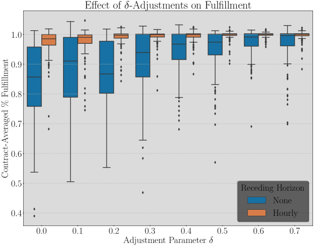
Figure 2: Risk Adjustment Simulations (Fulfillment)

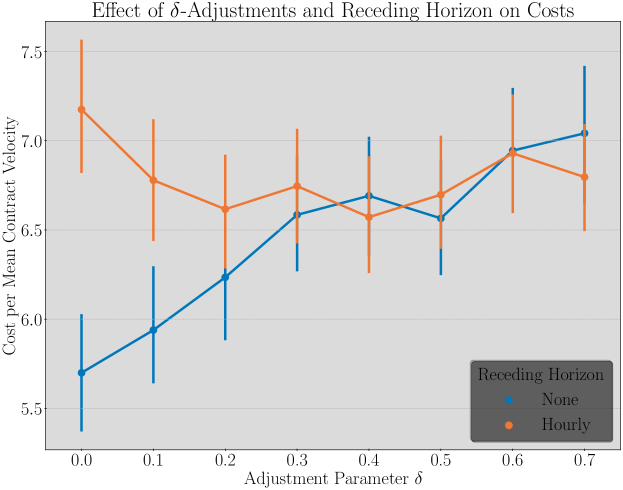
Figure 3: Risk Adjustment Simulations (Fulfillment)

3.3.3 Sensitivity Simulations

In order to illustrate the effects of a $\delta$ risk adjustment and the receding horizon re-calculations, we have carried out simulations similar to those of Section 3.2, however with smaller contracts $N=M=3$. The results are summarized by Figures 2 and 3.

Figure 2 provides a box plot comparing the parameter $\delta$ (applied to inflate the supply of each contract by the same proportion) to the average contract fulfillment (see $C_{a}^{(k)}$, Equation (19)). As is expected, the proportion of contracts which are completely fulfilled increases with $\delta$. In addition, the plot provides pairs of boxes comparing the results when the bids are updated only after a contract is fulfilled (this is the minimal update schedule that doesn’t overfill contracts), and when the bids are also updated every hour of simulation time (typically, about 20 updates are calculated over the simulation). An hourly receding horizon has a dramatic affect on the fulfillment – even without a risk adjustment, more than half of the contracts are fulfilled to at least $98\%$, and with a risk adjustment, almost all contracts are completely fulfilled.

Figure 3 provides a line plot similar to Figure 2 except the ordinate now quantifies the cost paid for items. Points are mean values across $500$ simulations and error bars are $98\%$ confidence intervals. In order to create a reasonable cost metric which is comparable across different contracts, we have normalized the total cost of attempting to fulfill a contract by that contract’s “mean velocity” requirement. To understand what we refer to as the velocity requirement, suppose that we are obligated to obtain $C$ items in $T$ time. Then, we define the velocity of this requirement by $v=C/T$. We take the mean velocity of the whole contract to be the average of the velocities of each individual requirement in the contract (in this case, over the $N=3$ requirements). To merely normalize by, e.g., the total number of items, would not result in a fair comparison since one contract may require obtaining the same number of items in less time (since they are generated randomly), which necessitates paying higher prices.

The main conclusions to be drawn from 3 are as follows. Firstly, without a receding horizon, there is naturally a tendency for costs to increase, since the supply acquisition is front-loaded. Secondly, as $\delta$ increases, the same upward pressure on costs is applicable as in the case without any receding horizon, but at the same time, for contracts which are difficult to fulfill, the receding horizon will drastically increase bids, which also increases the cost. However, for contracts which are easy to fulfill, or which get close to fulfillment early in the bidding period, the receding horizon smooths out the acquisition rate by reducing the bid, and therefore reducing costs. These are competing effects, but the use of the receding horizon is still able to reduce costs when $\delta$ is large; an ultimately small cost for achieving near complete fulfillment.

In summary, the receding horizon is able to achieve a much higher fulfillment proportion by increasing the bids (and incurring higher costs) for contracts which are difficult to fulfill (e.g., when supply rates are overestimated), while at the same time reducing the costs of fulfilling the remaining contracts by smoothing out bids that are too large.

4 Conclusions

This paper has studied the problem of minimum cost contract fulfillment in RTB auction markets. We have analyzed generalizations of the model proposed in [37] by considering both the first and second price auction mechanisms, and by allowing for general time-varying supply rate curves which can account for daily and weekly periodic cycles in market data. Moreover, we have uncovered the intrinsic convexity of the problem and provided a natural condition under which a strong duality result holds. Using duality, it has been shown that there is a close connection between the optimal bids $x(t)$ and certain dual variables which facilitates the complete representation of the optimal function $x(t)$ through the finite vector $\rho\in\mathbb{R}^{N}_{+}$ of dual variables. This close connection motivates the terminology “pseudo-bids” for the dual variables $\rho$. In the first price case, the optimal bids are obtained from $\rho$ by mapping them through a time-varying function quantifying the marginal costs of acquiring additional items; in the second price case (but not the first), the optimal bids are given exactly by $\rho$, which implies the optimal bids in this case are piecewise constant functions of time.

Further consequences of duality have lead to the conclusion (backed up with experimental simulation evidence) that there is in fact very little difference between the optimal solution in the first price or second price cases. This result has the important practical implication that, regardless of the type of auction one is participating in, they may as well assume that they are participating in a second price auction, which has been seen to always lead to a convex problem. Indeed, in second price auctions, the optimal bids are constant (corresponding exactly to the dual pseudo-bids $\rho$) and therefore the original time-independent formulation of [37] largely covers the general time-dependent case after calculating suitable time averages.

Finally, Section 3 develops methods for implementation and reports the results of simulation studies. A discretization method for Problem ($P$) is studied in Section 3.1 and we obtain a convergence rate for this discretization. The discretized problem is used in an empirical Monte Carlo study in Section 3.2, which demonstrates the similarity between optimal bidding in first and second price auctions. Further simulations in Section 3.3 demonstrate the effectiveness of $\delta$ supply inflation and receding horizon bid recalculation for ensuring that contracts are actually fulfilled in practice. Additional information regarding the practical implementation of these methods is provided in the appendix, with the basic ideas being summarized in Algorithm 1.

Appendix A Supply Rate Curve Estimation

In practice, the functions $W(x)$ will be estimated from available historical data. Therefore, depending on the method used to carry out this estimation, the resulting $\Lambda(x)$ is not necessarily guaranteed to be convex in the first price case (recall Proposition 2.2 requires $2$-concavity of $W$). If the estimate of $W(x)$ is simply carried out by fitting a particular parameterized distribution (e.g., a normal approximation) to a dataset, then there is unlikely to be any issue since most distributions commonly employed for this purpose do in fact have log-concave cumulative distribution functions. Moreover, since $W(x)$ arises through an auction process, extreme value theory and the Fisher-Tippett-Gnedenko Theorem may motivate the belief that $W(x)$ should tend to be close to a Weibull distribution, which is log-concave at least for some parameter ranges.

However, our empirical data (see also [27, 50]) suggests that such simple models are not good estimates for supply rate curves, and that the curves have a tendency towards some multi-modality. For this reason, the methods of Section 3.2 make use of Kernel density estimates (KDE). A Gaussian KDE model for $W(x)$ is natural because it ensures smoothness, that $W>0$, and the bandwidth can be chosen to correspond to the level of bid noise (or the level of bid noise can be chosen from the optimal KDE bandwidth).

Unfortunately, KDE estimates of $W(x)$ from data need not be (and often aren’t) log-concave or $\alpha$-concave. In order to deal with this problem, we consider calculating a convex and piecewise affine majorant of the function $\Lambda(s)$, which will transform Problem ($P_{K}$) into a linear program. A similar minorizing envelope can also be calculated through the methods of [30], and a piecewise minorant thereof computed by outer linear approximations. There is no obvious reason to prefer one approximation over the other and our experience has not demonstrated a clear benefit either way.

Alternatively, taking the log-concave envelope of $W(x)$ through similar methods is guaranteed to result in convex acquisition functions. The considerations of the previous paragraph suggest that we should at least expect the KDE estimates of $W$ to be “almost” log-concave, and indeed, this is what we have observed in our own experiments; the convex envelopes are only slight perturbations of the original supply rate curve estimate.

A.1 Piecewise Affine Approximation

Let us denote by $\widetilde{\Lambda}(x)$ the acquisition cost function attained from an estimated supply rate curve and by $\Lambda^{\mathsf{U}}(x)$ the minimal convex majorant $\widetilde{\Lambda}(x)$, i.e.,

$$\Lambda^{\mathsf{U}}(x)=\text{inf}\{\lambda(x)\ |\ \lambda(x)\geq\widetilde{\Lambda}(x),\lambda\text{ is convex and monotone increasing}\}.$$ (22)

We emphasize that $\lambda$ must be monotone increasing, but this would also follow as a consequence of the monotonicity of $\widetilde{\Lambda}$. The maximal minorant can be defined similarly. Moreover, $\alpha$-concave envelopes can be calculated by requiring that $\ell_{\alpha}\circ\lambda$ is convex.

A piecewise affine approximation of $\Lambda^{\mathsf{U}}$ can be found by discretizing a compact interval $[a,b]\subset\mathbb{R}$ into $n+1$ points $x_{0},x_{1},\ldots,x_{n}$ and solving the following convex quadratic program where convexity and monotonicity are enforced via finite differences

$$\underset{\lambda}{\mathrm{minimize}} \frac{1}{n+1}\sum_{i=0}^{n}\bigl{(}\lambda_{i}-\widetilde{\Lambda}(x_{i}))\bigr{)}^{2} E^{\mathsf{U}}$$ ()

$$\mathrm{subject\;to} \lambda_{i}\geq\widetilde{\Lambda}(x_{i})$$

$$\lambda_{i}-\lambda_{i-1}\geq 0\ \forall i\in[n]$$

$$\lambda_{i+1}-2\lambda_{i}+\lambda_{i-1}\geq 0\ \forall i\in[n-1].$$

An accurate approximation of the convex majorant is recovered via linearly interpolating $\lambda_{i}$. In fact, $\lambda_{i}$ will result in a strictly monotone function (and therefore a continuous inverse) whenever $\widetilde{\Lambda}$ is strictly monotone.

It is important that the developments in Section 2.4 do not make any assumptions regarding the differentiability of $W(x)$ or $\Lambda(s)$, since if these curves are corrected through solution of Problem ($E^{\mathsf{U}}$) to ensure convexity, it is by definition not differentiable. Moreover, simply interpolating the resulting $\lambda_{i}$ (e.g. with a cubic spline) may not be acceptable as, to our knowledge, it is not possible for this process to maintain simultaneously the monotonicity, convexity, and minorization of $\widetilde{W}$.

Remark A.1 (Sparse Approximations).

It is desirable to use a fine discretization in Problem ($E^{\mathsf{U}}$), otherwise the resulting function may fail to majorize $\widetilde{\Lambda}$ in regions of high curvature. However, each piecewise segment translates to an additional constraint when $\Lambda^{\mathsf{U}}$ is substituted into Problem ($P_{K}$) (see Section A.3), which may become overly burdensome for large problems. Therefore, it may be desirable to use a coarser approximation obtained by linearly interpolating samples of $\Lambda^{\mathsf{U}}(s)$. Since $\Lambda^{\mathsf{U}}(s)$ is convex, this process is guaranteed to produce another piecewise affine convex function which further majorizes $\Lambda^{\mathsf{U}}(s)$.

A.2 An Example

We consider an illustrative example of calculating log-concave envelopes of the supply rate curve in a simple market model. We suppose that each participant is characterized by a bid and rate pair $(b_{i},r_{i})$ indicating that they will bid $b_{i}$ with probability $r_{i}$ on any arriving item. We sample $\{(b_{i},r_{i})\}_{i=1}^{30}$ randomly as $b\sim\text{exp}(0.5)$ and $r_{i}\sim\beta(11.1,10)$ which represents a market with $30$ participants whose average bid is $0.5$ and have an average probability of $(11.1-10)/11.1\approx 0.1$ of bidding.

The bid landscape in this situation is given by

$$W(x)=\prod_{i:b_{i}>x}(1-r_{i}),$$

indicating the probability of winning an item if the bid $x$ is placed.

We let $\widetilde{W}(x)$ be a KDE smoothed (with $\sigma^{2}=1/4$) version of $W$ which corresponds either to the true supply rate curve under randomized bidding, or a reasonable estimate (from historical data) thereof. We denote supply rate curve estimates $\widetilde{W}^{\mathsf{L}}(x)$ and $\widetilde{W}_{\mathcal{N}}$ which are derived from $W(x)$ by solving Problem (22) for the function $-\text{log}\circ W$ and moment matching a Gaussian c.d.f., respectively. Note that this procedure produces minorants of the supply rate curve (and therefore majorants of the acquisition cost curve), since using a convex majorant procedure results in minorants of concave functions. Figure 4 plots examples of these functions and their associated cost and acquisition counterparts.

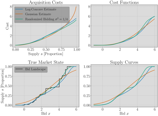
Figure 4: Example Supply Rate Functions

Comparison of different methods of estimating supply rate curves. Lower left: Comparison of KDE smoothing, the maximal log-concave minorant thereof, and a Gaussian c.d.f. (fit by moment matching) overlaid upon a true market state. Lower right: The three corresponding supply rate curves. Upper right: Corresponding cost curves. Upper left: Corresponding acquisition cost functions where we see that KDE smoothing does not lead to convexity, and that a Gaussian estimate is not a consistent minorant or majorant.

The examples of Figure 4 are chosen to deliberately exaggerate the differences between the supply curve estimates and the envelopes. For the simulation examples of Section 3.2 the two curves are often indistinguishable.

A.3 Linear Approximations of Primal Problem

From Section 3.1 we have the time discretized primal problem ($P_{K}$):

$$\underset{s,r}{\mathrm{minimize}} \sum_{j=1}^{M}\sum_{k:\widetilde{T}_{k}<T^{j}}\overline{\Lambda}_{jk}(s_{j}[k]) P_{K}$$ ()

$$\mathrm{subject\;to} \sum_{j\in\mathcal{A}_{i}}\sum_{k:\widetilde{T}_{k}<T^{j}}\Delta_{k}r_{ij}[k]\geq C_{i}$$

$$\sum_{i\in\mathcal{B}_{j}\cap\mathcal{T}_{T_{k}}}r_{ij}[k]=s_{j}[k]$$

$$r_{ij}[k]\geq 0.$$

Suppose that the functions $\Lambda_{j}(s,\widetilde{T}_{k})$ have piecewise affine approximations $\widehat{\Lambda}_{k}(s)=\underset{h\in H_{jk}}{\text{max}}\bigl{(}m_{hj}[k]s+b_{hj}[k]\bigr{)}$. Then, by introducing additional variables $\alpha_{jk}$ we can reformulate $P_{K}$ in epigraph form as a linear program

$$\underset{s,r}{\mathrm{minimize}} \frac{1}{2}\sum_{j=1}^{M}\sum_{k:\widetilde{T}_{k}\leq T^{j}}\Delta_{k}(\alpha_{jk}+\alpha_{j,k-1})$$ (23)

$$\mathrm{subject\;to} \sum_{j\in\mathcal{A}_{i}}\sum_{k:\widetilde{T}_{k}\leq T^{j}}\Delta_{k}r_{ij}[k]\geq C_{i}$$

$$m_{hj}[k]s_{j}[k]+b_{hj}[k]\leq\alpha_{jk}$$

$$\sum_{i\in\mathcal{B}_{j}\cap\mathcal{T}_{T_{k}}}r_{ij}[k]=s_{j}[k]$$

$$r_{ij}[k]\geq 0,$$

which is the formulation we have employed for our simulations in Section 3.2.

Appendix B Simulation (Additional Details)

In this section we provide additional details on the methods used to produce the results of Section 3.2.

B.1 Estimating Supply Rate Curves

The iPinYou dataset consists of impression data derived from a real DSP and includes information about bidding prices, market prices, and user characteristics. We focus on the season two data (a week long period $2013$-$06$-$06$ to $2013$-$06$-$12$). In all cases, our supply rate curve estimates are $24$h-periodic in time and therefore account for the natural daily (but not weekly) cycles in prices and arrival rates. Since this paper does not focus on the estimation of supply rate curves, we apply a simple estimation procedure using the entire dataset as input. Though this has the effect of leaking some information from the future, the estimation of supply rate curves is not subject to optimization, limiting the impact of this leakage. Moreover, the dataset is averaged into a single $24$h periodic function and extended through periodicity. It is reasonable to believe that the previous week’s (out of sample) data would provide similar results. Figure 5 provides an illustration of estimated supply rate curves where only $72$h of data is used to forecast the remaining $96$h for purposes of illustrating a case where historical data is used in this manner to forecast future trends.

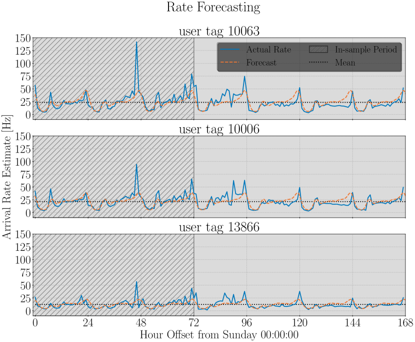
(a) Supply Rate $\lambda(t)$

(b) Win Probability Estimates

Figure 5: Estimated Supply Rate Curves and Costs

Cost and supply rate curves estimated from iPinYou data from the first 3 days of season 2. $(a)$ Item arrival rates and the corresponding forecasts. The hatched region indicates an in-sample period with the remainder being out-of-sample. Our simulations run on similar 3 day periods with a 12 hour sliding window for a total of 9 periods of 72 hours each. $(b)$ Estimates of the win probability function $\widetilde{W}(x,t)$ for $t=00:00:00$ (blue) and $t=09:00:00$ (red). We compare Gaussian KDE (solid line) with a parametric Exponential CDF (dashed line).

Provided with the iPinYou dataset is a user_tag which, according to [50] is “[a segment] in iPinYou’s proprietary audience database”. We therefore use the user_tag property as the “item types”, focusing on the five most common tags: 10063, 10006, 13866, 10024, and 10083.

B.2 Estimating the Supply Rate

In order to estimate the supply rate $\lambda_{j}(t)$ for each user tag, we have taken the inverse of the average of the time differences between arrival instants in each hour of the day, after removing outliers. Calculating the number of arrivals over an hour long period is not adequate as there appear to be large consistent gaps in arrival times: we suspect that the dataset was subsampled prior to being released.

This calculation results in estimates $\lambda_{j}[0],...,\lambda_{j}[23]$, with time denoted in hours. The continuous estimate was subsequently formed by smoothly interpolating between these points with a $24-$periodic boundary, resulting in a function $\tilde{\lambda}_{j}(t)$ defined on $[0,24]$. A forecast for the average supply rate at time $t$ is obtained via $\lambda_{j}(t)=\tilde{\lambda}(t\;\text{mod}\;24)$.

An illustrative example for tags 10063, 10006, and 13866 is provided in Figure 5(a).

B.3 Estimating Win Probabilities

Similarly to the supply rate estimates, we estimate an average win probability function for each $t\in{0,\ldots,23}$ and then smoothly interpolate along $t$ to estimate a $24-$periodic function $\widetilde{W}_{j}(x,t)$ indicating the probability of winning an impression of type (user tag) $j$ arriving at time $t$ given a bid $x$.

The estimate of $x\mapsto\widetilde{W}_{j}(x,t)$ is obtained by smoothing the histogram with a Gaussian kernel (bandwidth chosen simply by the Normal Reference Rule [42, Chap. 6.3]) for each market_price data point falling into the hour long window. The results of this procedure, as well as a comparison to a parametric estimate with an Exponential density are given in Figure 5(b).

The market_price attribute in the dataset corresponds to the price actually paid in the second price auction. We have not accounted for the affects of censoring; since the DSP collected the dataset with large bids intended to win most impressions that were bid on, this isn’t a significant factor.

B.4 Cost and Supply Rate Curves

The supply rate curve $W_{j}(x,t)$ is simply the product of the supply rate $\lambda_{j}(t)$ and the win probability $\widetilde{W}_{j}(x,t)$. The cost curves $f^{1st}$ and $f^{2nd}$ is derived from the supply rate curve using numerical integration and interpolation.

B.5 Simulating the Bidding Process

The simulations of Section 3.2 are obtained by storing the hour-by-hour inter-arrival and price data for each item type $j\in[M]$ and sampling uniformly from these datasets. At simulation time $t\in\mathbb{R}_{+}$ we sample an inter-arrival time $\Delta t$ and price $P$ from the data for hour $\lfloor t\rfloor+1$ with probability $t-\lfloor t\rfloor$ and otherwise from the data for hour $\lfloor t\rfloor$. A bid is solicited from a bidder (an implementation of ($P_{K}$)) and if the bid exceeds $P$ the bidder allocates that item to the fulfillment of a contract. The simulation time is them updated to $t+\Delta t$ and the process continues.

1

2

3

input : A Bidder derived from Section 3.1.

4

output : Recording of Bidder’s item allocations to process into normalized acquisition curves.

5

6// Initialize:

7 $Q\leftarrow\text{Priority-Queue}([\ ])$ // Sort by time

8 $t\leftarrow 0$ // The ‘‘current’’ time

9 for $j\in[M]$ do

10       // Sample an inter-arrival time and a price

11       $(\Delta t,P)\leftarrow\$Sample-Dataset($t$,$j$)

12       $Q$.push($(t+\Delta t,P,j)$)

13      

14

15// Simulate bidding process:

16 while $t<T_{\text{end}}$ do

17       $t,P,j\leftarrow Q$.pop()

18       $b\leftarrow\text{Bidder}$.solicit_bid($t$,$j$) // Ask for a bid on type $j$ at time $t$

19       if $b\geq P$ then

20             Bidder.award_item($t$,$j$) // Allocate items for winning bids

21            

22      $(\Delta t,P)\leftarrow\$Sample-Dataset($t$,$j$) // Append next $(t,P)$ pair for $j$ to $Q$

23       $Q$.push($(t+\Delta t,P,j)$)

24      

25

26 Function Sample-Dataset($t$,$j$):

27       $p\leftarrow t-\lfloor t\rfloor$

28       $U\sim\mathcal{U}(0,1)$ // Interpolate between hours

29       if $p\leq U$ then

30             $h\leftarrow\lfloor t\rfloor$

31            

32      else

33             $h\leftarrow\lfloor t\rfloor+1$

34            

35      $\Delta t\leftarrow$ Sample-Inter-arrivals(hour=$h$,type=$j$)

36       $P\leftarrow$ Sample-Prices(hour=$h$,type=$j$)

37       return $(\Delta t,P)$

38      

Algorithm 2 Bidding Simulation

Appendix C Proofs

C.1 Proofs of Main Results

[main]

C.2 Additional Proofs

[aux] [aux2]

References

- [1] Akshay Agrawal, Robin Verschueren, Steven Diamond and Stephen Boyd “A rewriting system for convex optimization problems” In Journal of Control and Decision 5.1, 2018, pp. 42–60
- [2] Santiago R Balseiro, Omar Besbes and Gabriel Y Weintraub “Repeated auctions with budgets in ad exchanges: Approximations and design” In Management Science 61.4 INFORMS, 2015, pp. 864–884
- [3] Santiago R Balseiro and Yonatan Gur “Learning in repeated auctions with budgets: Regret minimization and equilibrium” In Management Science 65.9 INFORMS, 2019, pp. 3952–3968
- [4] Dimitri P Bertsekas “Extended monotropic programming and duality” In Journal of optimization theory and applications 139.2 Springer, 2008, pp. 209–225
- [5] Stephen Boyd and Lieven Vandenberghe “Convex Optimization” Cambridge University Press, 2004 URL: https://web.stanford.edu/~boyd/cvxbook/
- [6] Pornpawee Bumpensanti and He Wang “A re-solving heuristic with uniformly bounded loss for network revenue management” In Management Science 66.7 INFORMS, 2020, pp. 2993–3009
- [7] Han Cai et al. “Real-Time Bidding by Reinforcement Learning in Display Advertising.” In CoRR abs/1701.02490, 2017 URL: http://dblp.uni-trier.de/db/journals/corr/corr1701.html#CaiRZMWYG17
- [8] Ye Chen, Pavel Berkhin, Bo Anderson and Nikhil R. Devanur “Real-time bidding algorithms for performance-based display ad allocation.” In KDD ACM, 2011, pp. 1307–1315 URL: http://dblp.uni-trier.de/db/conf/kdd/kdd2011.html#ChenBAD11
- [9] Francis Clarke “Functional analysis, calculus of variations and optimal control” 264, Graduate Texts in Mathematics Springer Science & Business Media, 2013 DOI: 10.1007/978-1-4471-4820-3
- [10] Robert M Corless et al. “On the LambertW function” In Advances in Computational mathematics 5.1 Springer, 1996, pp. 329–359
- [11] Ying Cui, Ruofei Zhang, Wei Li and Jianchang Mao “Bid landscape forecasting in online ad exchange marketplace.” In KDD ACM, 2011, pp. 265–273 URL: http://dblp.uni-trier.de/db/conf/kdd/kdd2011.html#CuiZLM11
- [12] Steven Diamond and Stephen Boyd “CVXPY: A Python-embedded modeling language for convex optimization” In Journal of Machine Learning Research 17.83, 2016, pp. 1–5
- [13] Joaquin Fernandez-Tapia, Olivier Guéant and Jean-Michel Lasry “Optimal real-time bidding strategies” In Applied Mathematics Research eXpress 2017.1 Oxford University Press, 2017, pp. 142–183
- [14] Bruno Gaujal, Nicolas Navet and Cormac Walsh “Shortest-path algorithms for real-time scheduling of FIFO tasks with minimal energy use” In ACM Transactions on Embedded Computing Systems (TECS) 4.4 ACM New York, NY, USA, 2005, pp. 907–933
- [15] Aritra Ghosh et al. “Scalable Bid Landscape Forecasting in Real-time Bidding.” In CoRR abs/2001.06587, 2020 URL: http://dblp.uni-trier.de/db/journals/corr/corr2001.html#abs-2001-06587
- [16] Arpita Ghosh, Benjamin I.. Rubinstein, Sergei Vassilvitskii and Martin Zinkevich “Adaptive bidding for display advertising.” In WWW ACM, 2009, pp. 251–260 URL: http://dblp.uni-trier.de/db/conf/www/www2009.html#GhoshRVZ09
- [17] Nicolas Grislain, Nicolas Perrin and Antoine Thabault “Recurrent Neural Networks for Stochastic Control in Real-Time Bidding.” In KDD ACM, 2019, pp. 2801–2809 URL: http://dblp.uni-trier.de/db/conf/kdd/kdd2019.html#GrislainPT19
- [18] R. Gummadi, Peter B. Key and Alexandre Proutière “Optimal bidding strategies in dynamic auctions with budget constraints.” In Allerton IEEE, 2011, pp. 588 URL: http://dblp.uni-trier.de/db/conf/allerton/allerton2011.html#GummadiKP11
- [19] IAB “IAB internet advertising revenue report conducted by PricewaterhouseCoopers (PWC)”, 2018 URL: https://www.iab.com/insights
- [20] Krishnamurthy Iyer, Ramesh Johari and Mukund Sundararajan “Mean field equilibria of dynamic auctions with learning” In Management Science 60.12 INFORMS, 2014, pp. 2949–2970
- [21] Niklas Karlsson “Adaptive control using Heisenberg bidding.” In ACC IEEE, 2014, pp. 1304–1309 URL: http://dblp.uni-trier.de/db/conf/amcc/acc2014.html#Karlsson14
- [22] Niklas Karlsson “Control problems in online advertising and benefits of randomized bidding strategies” In European Journal of Control 30 Elsevier, 2016, pp. 31–49
- [23] Niklas Karlsson “Plant gain estimation in online advertising processes.” In CDC IEEE, 2017, pp. 2182–2187 URL: http://dblp.uni-trier.de/db/conf/cdc/cdc2017.html#Karlsson17
- [24] Vijay Krishna “Auction Theory” Academic Press, 2002
- [25] Wook Hyun Kwon and Soo Hee Han “Receding horizon control: model predictive control for state models” Springer Science & Business Media, 2006
- [26] Larry J Leblanc and Leon Cooper “The transportation-production problem” In Transportation Science 8.4 INFORMS, 1974, pp. 344–354
- [27] Hairen Liao, Lingxiao Peng, Zhenchuan Liu and Xuehua Shen “iPinYou Global RTB Bidding Algorithm Competition Dataset.” In ADKDD@KDD ACM, 2014, pp. 6:1–6:6 URL: http://dblp.uni-trier.de/db/conf/kdd/adkdd2014.html#LiaoPLS14
- [28] Yishay Mansour, S. Muthukrishnan and Noam Nisan “Doubleclick Ad Exchange Auction” In CoRR abs/1204.0535, 2012 URL: http://dblp.uni-trier.de/db/journals/corr/corr1204.html#abs-1204-0535
- [29] Flavio M Menezes and Paulo Klinger Monteiro “An introduction to auction theory” OUP Oxford, 2005
- [30] Adam Oberman “The convex envelope is the solution of a nonlinear obstacle problem” In Proceedings of the American Mathematical Society 135.6, 2007, pp. 1689–1694
- [31] Art B. Owen “Monte Carlo theory, methods and examples”, 2013 URL: http://statweb.stanford.edu/~owen/mc/
- [32] Claudia Perlich et al. “Bid optimizing and inventory scoring in targeted online advertising.” In KDD ACM, 2012, pp. 804–812 URL: http://dblp.uni-trier.de/db/conf/kdd/kdd2012.html#PerlichDHSRP12
- [33] Ana Radovanovic and William D. Heavlin “Risk-aware revenue maximization in display advertising.” In WWW ACM, 2012, pp. 91–100 URL: http://dblp.uni-trier.de/db/conf/www/www2012.html#RadovanovicH12
- [34] Michael H. Schneider “Network flows and monotropic optimization” In Networks 16.4, 1986, pp. 441–443 URL: http://dblp.uni-trier.de/db/journals/networks/networks16.html#Schneider86
- [35] J Frank Sharp, James C Snyder and James H Greene “A decomposition algorithm for solving the multifacility production-transportation problem with nonlinear production costs” In Econometrica: Journal of the Econometric Society JSTOR, 1970, pp. 490–506
- [36] Elias M Stein and Rami Shakarchi “Real analysis: measure theory, integration, and Hilbert spaces” Princeton University Press, 2009
- [37] Erik Tillberg, Peter Marbach and Ravi Mazumdar “An Optimal Bidding Algorithm for Online Ad Auctions with Overlapping Targeting Criteria” In Proc. ACM Meas. Anal. Comput. Syst. 4.2 New York, NY, USA: Association for Computing Machinery, 2020 DOI: 10.1145/3366707
- [38] Pauli Virtanen et al. “SciPy 1.0: Fundamental Algorithms for Scientific Computing in Python” In Nature Methods 17, 2020, pp. 261–272
- [39] Jun Wang, Weinan Zhang and Shuai Yuan “Display advertising with real-time bidding (RTB) and behavioural targeting” In Foundations and Trends® in Information Retrieval 11.4-5 Now Publishers, Inc., 2017, pp. 297–435
- [40] Yining Wang and He Wang “Constant Regret Re-solving Heuristics for Price-based Revenue Management” In arXiv preprint arXiv:2009.02861, 2020
- [41] Yuchen Wang et al. “Functional Bid Landscape Forecasting for Display Advertising.” In ECML/PKDD (1) 9851, Lecture Notes in Computer Science Springer, 2016, pp. 115–131 URL: http://dblp.uni-trier.de/db/conf/pkdd/pkdd2016-1.html#WangRZWY16
- [42] Larry Wasserman “All of nonparametric statistics” Springer Science & Business Media, 2006 DOI: 10.1007/0-387-30623-4
- [43] Di Wu et al. “Budget constrained bidding by model-free reinforcement learning in display advertising” In Proceedings of the 27th ACM International Conference on Information and Knowledge Management, 2018, pp. 1443–1451
- [44] Wush Chi-Hsuan Wu, Mi-Yen Yeh and Ming-Syan Chen “Predicting Winning Price in Real Time Bidding with Censored Data.” In KDD ACM, 2015, pp. 1305–1314 URL: http://dblp.uni-trier.de/db/conf/kdd/kdd2015.html#WuYC15
- [45] Wush Chi-Hsuan Wu, Mi-Yen Yeh and Ming-Syan Chen “Deep Censored Learning of the Winning Price in the Real Time Bidding.” In KDD ACM, 2018, pp. 2526–2535 URL: http://dblp.uni-trier.de/db/conf/kdd/kdd2018.html#WuYC18
- [46] Shuai Yuan, Jun Wang and Xiaoxue Zhao “Real-time bidding for online advertising: measurement and analysis” In Proceedings of the Seventh International Workshop on Data Mining for Online Advertising, 2013, pp. 1–8
- [47] Weinan Zhang et al. “Feedback Control of Real-Time Display Advertising.” In WSDM ACM, 2016, pp. 407–416 URL: http://dblp.uni-trier.de/db/conf/wsdm/wsdm2016.html#ZhangRWZW16
- [48] Weinan Zhang and Jun Wang “Statistical Arbitrage Mining for Display Advertising.” In KDD ACM, 2015, pp. 1465–1474 URL: http://dblp.uni-trier.de/db/conf/kdd/kdd2015.html#ZhangW15a
- [49] Weinan Zhang, Shuai Yuan and Jun Wang “Optimal real-time bidding for display advertising.” In KDD ACM, 2014, pp. 1077–1086 URL: http://dblp.uni-trier.de/db/conf/kdd/kdd2014.html#ZhangYW14
- [50] Weinan Zhang, Shuai Yuan, Jun Wang and Xuehua Shen “Real-time bidding benchmarking with ipinyou dataset” In arXiv preprint arXiv:1407.7073, 2014
- [51] Weinan Zhang, Tianxiong Zhou, Jun Wang and Jian Xu “Bid-aware Gradient Descent for Unbiased Learning with Censored Data in Display Advertising.” In KDD ACM, 2016, pp. 665–674 URL: http://dblp.uni-trier.de/db/conf/kdd/kdd2016.html#ZhangZWX16
- [52] Wen-Yuan Zhu et al. “A gamma-based regression for winning price estimation in real-time bidding advertising.” In BigData IEEE Computer Society, 2017, pp. 1610–1619 URL: http://dblp.uni-trier.de/db/conf/bigdataconf/bigdataconf2017.html#ZhuSLPH17