Multicenter integrals involving complex Gaussian type functions

Abstract

Multicentric integrals that involve a continuum state cannot be evaluated with the usual quantum chemistry tools and require a special treatment. We consider an initial molecular bound state described by multicenter spherical or cartesian Gaussian functions. An electron ejected through an ionization process will be described by an oscillating continuum wavefunction that enters the matrix element necessary for cross section calculations. Within a monocentric approach, we have recently shown how such integrals can be evaluated analytically by using a representation of the continuum state by a set of complex Gaussian functions. In this work we tackle the multicentric situation. The method, developed in either spherical or cartesian coordinates, and validated by numerical tests, makes use of existing mathematical tools extended to the complex plane.

1 Introduction

There exists a vast literature dedicated to the evaluation of integrals necessary in quantum chemistry and in molecular physics. According to the type of functions involved (like Gaussian-type or Slater-type, correlated or not correlated, and in diverse coordinate systems) specific strategies may be envisaged. Within the realm of bound states, in particular, Gaussians play a particular role since they are commonly used by a large number of chemists and physicists alike [1]. The main reason for this widespread use is that Gaussians possess very nice properties, including the famous product theorem [2]; they greatly facilitate the evaluation of multicenter integrals that appear in molecular studies.

When continuum states (or even highly excited states) are involved, as in scattering problems, integrals are more difficult to evaluate because of oscillating integrands spanning generally a more extended radial range. Besides, Gaussian-type functions are not a natural basis choice for continuum states. Indeed, radial functions oscillating up to infinity are difficult to represent by fast decaying Gaussians. This option has been explored only in few studies [3, 4, 5], since least square real Gaussian representations turn out to be relatively inefficient in reproducing the oscillations at large radial distance and high energy (typically $r\sim 15-20$ a.u. and $E\sim 1.5-2$ a.u. for a regular Coulomb function, as an example). Alternatively, complex Gaussians, i.e. Gaussian functions with complex exponents, could be more appropriate for continuum calculations because they intrinsically oscillate. Since McCurdy and Rescigno [6] proposed their use as an alternative to the complex-coordinate technique, complex Gaussians have been applied to study ionization cross sections [7, 8, 9, 10, 11, 12, 13] and molecular resonances [14, 15], and even for non-Born-Oppenheimer ground and excited states calculations (see [16] and references therein). In a recent study [17, 18], we have developed an efficient numerical approach to represent a set of oscillating functions over a finite range by optimized complex Gaussians. We have also performed a detailed comparison between using complex and real Gaussians, and we can summarize our findings as follows: complex Gaussians are better suited for oscillating functions (in particular for larger energies), allow one to cover larger radial domains with greater accuracy and avoid unphysical behaviors outside the fitting box. Returning to the goal of evaluating efficiently integrals involved in scattering processes, we have shown [17, 18] that a complex Gaussian representation of continuum states allows for an analytical approach, as long as one stays within a monocentric framework.

The idea of the present work is to show how to extend the method when matrix elements include multicentric molecular integrals over continuum states. If the bound state is described in terms of real Gaussians, our continuum state representation by optimized complex Gaussians leads to an all-Gaussian approach that can take advantage of the Gaussian properties, similar to what is done in quantum chemistry. In the one active electron approach we wish to compute efficiently matrix elements like

$$\mathcal{T}_{\mathbf{k_{e}}}=\braket{\psi_{\mathbf{k_{e}}}\left(\mathbf{r}-\mathbf{O}\right)}{\widehat{O}}{\Phi_{i}\left(\mathbf{r}-\mathbf{R}\right)},$$ (1)

where $\Phi_{i}$ is an initial bound state centered around a position $\mathbf{R}$, $\psi_{\mathbf{k_{e}}}$ is a continuum state (with a wavevector $\mathbf{k_{e}}$) centered around a position $\mathbf{O}$, and $\widehat{O}$ is an operator. To illustrate the usefulness of representing continuum with complex Gaussians, we have started with a simpler problem, in which both states are centered on the origin of the coordinate system [17, 18]. Also, to compare with a solid and exact benchmark, we first considered the cross section calculation of the photoionization of atomic hydrogen for which all wavefunctions involved are known analytically ($\widehat{O}$ is just the dipole operator). Through a complex Gaussian representation of the radial part of the continuum, and a real Gaussian expansion of a given exact initial state $nl$, the matrix element becomes fully analytical. Actually it turns out that, although mathematically different, the matrix element calculation is also analytical if the initial state is described by Slater-type orbitals. Next, we have considered the photoionization of molecules, whose initial and final states are described in a one-centre approach [18, 19]. The strategy works as well when the operator is replaced by a plane wave ($e^{\imath\mathbf{q}\cdot\mathbf{r}}$) that appears, within the first Born approximation, when evaluating cross sections for ionization by a charged particle impact ($\mathbf{q}$ is the momentum transferred to the target). In all cases, the numerically demanding part is the non-linear optimization of complex Gaussians to represent the continuum. The matrix elements, expressed as multiple limited sums involving special functions, are easily computed. The successful numerical comparison illustrated that the proposed all-Gaussian approach works efficiently for ionization processes of one-center targets.

In the present paper, we wish to show that we can go a step further towards a multicentric case, still retaining the analytical character of the approach. Following the quantum chemistry strategy used for bound states we make use of Gaussians properties. When applying the product theorem with complex Gaussians, though, one major issue is that we are faced with complex centers. Thus, the study of such matrix elements is not a mere extension of the monocentric case but involves some more advanced mathematical tools that we present hereafter.

In the next section we provide the proposed formulation for either spherical or cartesian Gaussian functions. A numerical test case is then presented in Section 3, and our findings are summarized in Section 4.

2 Analytical evaluation of transition matrix elements

Consider the photoionization of a molecule. Initially in the electronic state $\Phi_{i}$, it is ionized by a photon of energy $\omega$ and a polarization vector $\epsilon$, say, chosen along of z-axis ($\epsilon=\hat{z}$). We suppose that the vibrational and rotational structure of molecule is not affected in the process. Let the ejected electron have an energy $k_{e}^{2}/2$ and a wavevector $\mathbf{k_{e}}$. Its continuum state $\psi_{\mathbf{k_{e}}}$ is supposed, for simplicity, to be centered on the origin $\mathbf{O}=\mathbf{0}$. The initial molecular state will have several centers. However, for our purposes, it will be sufficient to take a single function $\Phi_{i}\left(\mathbf{r}-\mathbf{R}\right)$ centered on a vector $\mathbf{R}\equiv\left(X,Y,Z\right)$.

Within the dipole approximation, the transition moment is given by

$$\mathcal{T}_{\mathbf{k_{e}}}^{(g)}=\braket{\psi_{\mathbf{k_{e}}}\left(\mathbf{r}\right)}{\widehat{O}^{(g)}}{\Phi_{i}\left(\mathbf{r}-\mathbf{R}\right)},$$ (2)

where the dipole operator in length $(L)$ or velocity $(V)$ gauge reads

$$\widehat{O}^{(L)} =\hat{\epsilon}\cdot\mathbf{r}=z=\sqrt{\frac{4\pi}{3}}rY_{1}^{0}\left(\hat{r}\right),$$ (3)

$$\widehat{O}^{(V)} =-\frac{\imath}{w}\hat{\epsilon}\cdot\mathbf{p}=-\frac{\imath}{\omega}p_{z},$$

where $Y_{l}^{m}$ is the usual spherical harmonic. If exact wavefunctions are used, the two gauges are equivalent, and results of the calculations coincide. In this paper, we shall consider only the length gauge formulation.

We expand the continuum wavefunction in partial waves

$$\psi_{\mathbf{k_{e}}}(\mathbf{r})=\sqrt{\frac{2}{\pi}}\sum_{l=0}^{\infty}\sum_{m=-l}^{l}(\imath)^{l}e^{-\imath\sigma_{l}}\frac{u_{l,k_{e}}(r)}{k_{e}r}Y_{l}^{m}(\hat{r})Y_{l}^{m*}\left(\widehat{k_{e}}\right),$$ (4)

where the radial functions $u_{l,k_{e}}(r)$ are the solutions of the radial Schrödinger equation, and $\sigma_{l}$ are the corresponding phase-shifts. As suggested in [17], these radial functions can be represented by a set of $N$ optimized complex Gaussians,

$$\left(u_{l,k_{e}}(r)\right)^{*}=r^{l+1}\sum_{s=1}^{N}\left[c_{s}\right]_{l,k_{e}}e^{-\left[\alpha_{s}\right]_{l}r^{2}}.$$ (5)

The non-linear exponents $\left[\alpha_{s}\right]_{l}$ and the linear coefficients $\left[c_{s}\right]_{l,k_{e}}$ are here supposed to be already known.

For the initial state $\Phi_{i}\left(\mathbf{r}-\mathbf{R}\right)$, we consider here two different Gaussian-type functions: $(i)$ the spherical Gaussian-type functions (SGTFs) in section 2.1; and $(ii)$ the cartesian Gaussian-type functions (CGTFs) in section 2.2. In both cases, we will show that the matrix element (2) can be evaluated analytically. We also emphasize here that if $\mathbf{R}=\mathbf{0}$, that is to say in the monocentric case, the formulation developed hereafter reduces to that presented in [17, 18].

2.1 Spherical Gaussian-type functions

We suppose here that the initial state is a SGTF

$$\Phi_{n_{i}l_{i}m_{i}}(\mathbf{r})=\mathbb{Y}_{l_{i}m_{i}}^{n_{i}}(\mathbf{r})e^{-\beta_{i}r^{2}},$$ (6)

where

$$\mathbb{Y}_{l_{i}m_{i}}^{n_{i}}(\mathbf{r})=\left(\mathbf{r}\cdot\mathbf{r}\right)^{n_{i}}\mathcal{Y}_{l_{i}}^{m_{i}}(\mathbf{r}),$$ (7)

is the general harmonic polynomial and $\mathcal{Y}_{l}^{m}$ is the solid harmonic.

For real argument $\mathbf{r}\in\mathbb{R}^{3}$, the latter is given in terms of the usual spherical harmonic

$$\mathcal{Y}_{l}^{m}(\mathbf{r})=r^{l}Y_{l}^{m}(\hat{r}),$$ (8)

while for complex arguments $\mathbf{r}\equiv(x,y,z)\in\mathbb{C}^{3}$, it becomes [20]

$$\mathcal{Y}_{l}^{m}\left(\mathbf{r}\right)=\sqrt{\frac{2l+1}{4\pi}(l+m)!(l-m)!}\sum_{k}\frac{(-x-\imath y)^{k+m}(x-\imath y)^{k}(z)^{l-2k-m}}{2^{2k+m}(k+m)!\,k!\,(l-m-2k)!}.$$ (9)

Note that the integer number $n_{i}$ is not a quantum number; it allows one to consider different types of Gaussian functions. The very commonly employed s-type Gaussian corresponds to $n_{i}=l_{i}=0$.

Molecular integrals involving SGTF with real arguments were considered by Harris [21] and Krauss [22]; they can be performed analytically by repeatedly rotating the spherical harmonics. Fieck [23] evaluated multicenter integrals by using the Talmi transformation and the Moshinsky-Smirnov coefficients of nuclear shell theory. Kaufmann and Baumeister [24] derived a single center expansion for an arbitrary Gaussian and used the modified Rayleigh expansion. Chiu and Moharerrzadeh [25] applied a similar strategy in which they used a translational and rotational expansion of the Gaussian from one center to another. They then treated the two-electron integrals by using the Fourier transformation convolution theorem [26]. Kuang and Lin [27] derived analytical results for multicenter integrals over SGTFs by using the Fourier transform and the addition theorem of harmonic polynomials. They also apply the same approach to treat molecular integrals involving also a plane wave [28]. For this purpose, they generalized the addition theorem of harmonic polynomials for complex arguments. In this section, we will use this generalization to obtain an analytical expression for the transition element (2). We will first consider the special case $n_{i}=0$ which is very common in quantum chemistry and allows one to master the necessary mathematical steps. Then we will move on to the general case $n_{i}\geq 0$.

2.1.1 Special case: $n_{i}=0$

We consider here the transition matrix element (2) (in the length gauge)

$$\mathcal{T}^{(L)}_{\mathbf{k_{e}}} =\braket{\psi_{\mathbf{k_{e}}}\left(\mathbf{r}\right)}{\sqrt{\frac{4\pi}{3}}rY_{1}^{0}\left(\hat{r}\right)}{\Phi_{n_{i}=0\,l_{i}m_{i}}\left(\mathbf{r}-\mathbf{R}\right)}$$ (10)

$$=\frac{2\sqrt{2}}{k_{e}\sqrt{3}}\sum_{l,m}(-\imath)^{l}e^{\imath\sigma_{l}}Y_{l}^{m}\left(\widehat{k_{e}}\right)\mathcal{J}_{l,m},$$

with

$$\mathcal{J}_{l,m} =\int d\mathbf{r}\left(u_{l,k_{e}}(r)\right)^{*}Y_{l}^{m*}(\hat{r})\,Y_{1}^{0}(\hat{r})\,e^{-\beta_{i}\left(\mathbf{r}-\mathbf{R}\right)^{2}}\mathcal{Y}_{l_{i}}^{m_{i}}\left(\mathbf{r}-\mathbf{R}\right).$$ (11)

To evaluate this three-dimensional integral, we make use of two mathematical ingredients. First, the addition theorem for solid harmonics [29]

$$\mathcal{Y}_{l_{i}}^{m_{i}}(\mathbf{r}-\mathbf{R})=4\pi\sum_{l^{\prime}=0}^{l_{i}}\sum_{m^{\prime}=m_{\min}^{\prime}}^{m_{\max}^{\prime}}G(l_{i}\,m_{i}|l^{\prime}\,m^{\prime})\mathcal{Y}_{l^{\prime}}^{m^{\prime}}(\mathbf{r})\mathcal{Y}_{l_{i}-l^{\prime}}^{m_{i}-m^{\prime}}(-\mathbf{R}),$$ (12)

with $m_{\min}^{\prime}=\max(-l^{\prime},m_{i}-l_{i}+l^{\prime})$, $m_{\max}^{\prime}=\min(l^{\prime},m_{i}+l_{i}-l^{\prime})$, and

$$G(l_{i}\,m_{i}|l^{\prime}\,m^{\prime})=\frac{(2l_{i}+1)!!}{(2l^{\prime}+1)!!\left[2(l_{i}-l^{\prime})+1\right]!!}\braket{l_{i}\,m_{i}}{l^{\prime}\,m^{\prime}}{l_{i}-l^{\prime}\,,m_{i}-m^{\prime}}$$ (13)

where $\braket{l_{2}\,m_{2}}{L\,M}{l_{1}\,m_{1}}$ denotes the Gaunt coefficient

$$\braket{l_{2}\,m_{2}}{L\,M}{l_{1}\,m_{1}}=\int d\hat{r}Y_{l_{2}}^{m_{2}*}\left(\hat{r}\right)Y_{L}^{M}\left(\hat{r}\right)Y_{l_{1}}^{m_{1}}\left(\hat{r}\right).$$ (14)

Second, we need the expansion formula [28]

$$e^{2\beta_{i}\mathbf{r}\cdot\mathbf{R}}=4\pi\sum_{\lambda=0}^{\infty}\sum_{\mu=-\lambda}^{\lambda}(-1)^{\mu}\mathcal{Y}_{\lambda}^{\mu}\left(\mathbf{r}\right)\mathcal{Y}_{\lambda}^{-\mu}\left(2\beta_{i}\mathbf{R}\right)\sum_{k=0}^{\infty}\frac{\left(\mathbf{r}\cdot\mathbf{r}\right)^{k}\left[2\beta_{i}\mathbf{R}\cdot 2\beta_{i}\mathbf{R}\right]^{k}}{(2k)!!(2k+2\lambda+1)!!}.$$ (15)

Applying the homogeneous property $\mathcal{Y}_{l}^{m}\left(\gamma\mathbf{r}\right)=\gamma^{l}\mathcal{Y}_{l}^{m}\left(\mathbf{r}\right)$, we can write
$\mathcal{Y}_{\lambda}^{-\mu}\left(2\beta_{i}\mathbf{R}\right)=2^{\lambda}\mathcal{Y}_{\lambda}^{-\mu}\left(\beta_{i}\mathbf{R}\right)$.

Inserting formulae (12) and (15), and replacing the radial function of the continuum by its Gaussian representation (5), the integral (11) becomes

$$\mathcal{J}_{l,m} =\left(4\pi\right)^{2}e^{-\beta_{i}R^{2}}\sum_{s=1}^{N}\left[c_{s}\right]_{l,k_{e}}\sum_{l^{\prime}=0}^{l_{i}}\sum_{m^{\prime}=m_{\min}^{\prime}}^{m_{\max}^{\prime}}G(l_{i}\,m_{i}|l^{\prime}\,m^{\prime})\mathcal{Y}_{l_{i}-l^{\prime}}^{m_{i}-m^{\prime}}(-\mathbf{R})$$ (16)

$$\quad\times\sum_{\lambda=0}^{\infty}\sum_{\mu=-\lambda}^{\lambda}(-1)^{\mu}2^{\lambda}\mathcal{Y}_{\lambda}^{-\mu}\left(\beta_{i}\mathbf{R}\right)\int d\hat{r}\,Y_{l}^{m*}(\hat{r})\,Y_{1}^{0}(\hat{r})\,{Y}_{l^{\prime}}^{m^{\prime}}(\hat{r}){Y}_{\lambda}^{\mu}\left(\hat{r}\right)$$

$$\quad\times\sum_{k=0}^{\infty}\frac{\left[2\beta_{i}\mathbf{R}\cdot 2\beta_{i}\mathbf{R}\right]^{k}}{(2k)!!(2k+2\lambda+1)!!}\int_{0}^{\infty}d{r}\,r^{l+l^{\prime}+\lambda+2k+3}e^{-\left(\left[\alpha_{s}\right]_{l}+\beta_{i}\right)r^{2}}.$$

The angular integral over four spherical harmonics can be seen to give

$$\sum_{d=|l^{\prime}-1|}^{l^{\prime}+1}\braket{l\,m}{\lambda\,\mu}{d\,,m-\mu}\braket{l^{\prime}\,m^{\prime}}{1\,0}{d\,m^{\prime}}\delta_{m^{\prime},m-\mu},$$ (17)

with the conditions $|l-d|\leq\lambda\leq l+d$, $l^{\prime}+1+d=\text{even integer}$ ($d\neq l^{\prime}$) and $l+\lambda+d=\text{even integer}$. The radial integral is quite straightforward, and the summation over $k$ can be carried out, and yields a confluent hypergeometric function ${}_{1}F_{1}$ [30], namely

$$\sum_{k=0}^{\infty}\frac{\left[2\beta_{i}\mathbf{R}\cdot 2\beta_{i}\mathbf{R}\right]^{k}}{(2k)!!(2k+2\lambda+1)!!}\int_{0}^{\infty}d{r}\,r^{l+l^{\prime}+\lambda+2k+3}e^{-\left(\left[\alpha_{s}\right]_{l}+\beta_{i}\right)r^{2}}$$ (18)

$$= \sum_{k=0}^{\infty}\frac{\left[2\beta_{i}\mathbf{R}\cdot 2\beta_{i}\mathbf{R}\right]^{k}}{\frac{2^{2k+\lambda+1}}{\sqrt{\pi}}\Gamma\left(k+1\right)\Gamma\left(k+\lambda+\frac{3}{2}\right)}\frac{\Gamma\left(k+\frac{l+l^{\prime}+\lambda+4}{2}\right)}{2\left(\left[\alpha_{s}\right]_{l}+\beta_{i}\right)^{k+\frac{l+l^{\prime}+\lambda+4}{2}}}$$

$$= \frac{\sqrt{\pi}\,\Gamma\left(\frac{l+l^{\prime}+\lambda+4}{2}\right)}{2^{\lambda+2}\Gamma\left(\lambda+\frac{3}{2}\right)\left(\left[\alpha_{s}\right]_{l}+\beta_{i}\right)^{\frac{l+l^{\prime}+\lambda+4}{2}}}\,_{1}F_{1}\left(\frac{l+l^{\prime}+\lambda+4}{2},\lambda+\frac{3}{2};\frac{\beta_{i}^{2}R^{2}}{\left[\alpha_{s}\right]_{l}+\beta_{i}}\right).$$

Collecting the results of the two integrations gives us the following final expression for the integral $\mathcal{J}_{l,m}$

$$\mathcal{J}_{l,m} =4\pi^{2}\sqrt{\pi}(-1)^{m}\,(2l_{i}+1)!!\,e^{-\beta_{i}R^{2}}\sum_{l^{\prime}=0}^{l_{i}}\frac{1}{(2l^{\prime}+1)!!\left[2(l_{i}-l^{\prime})+1\right]!!}$$ (19)

$$\quad\times\sum_{m^{\prime}=m_{\min}^{\prime}}^{m_{\max}^{\prime}}(-1)^{m^{\prime}}\braket{l_{i}\,m_{i}}{l^{\prime}\,m^{\prime}}{l_{i}-l^{\prime}\,,m_{i}-m^{\prime}}\mathcal{Y}_{l_{i}-l^{\prime}}^{m_{i}-m^{\prime}}(-\mathbf{R})$$

$$\quad\times\sum_{d=|l^{\prime}-1|}^{l^{\prime}+1}\braket{l^{\prime}\,m^{\prime}}{1\,0}{d\,m^{\prime}}\sum_{\lambda=|l-d|}^{l+d}\braket{l\,m}{\lambda\,,m-m^{\prime}}{d\,,m^{\prime}}$$

$$\quad\times\frac{\Gamma\left(\frac{l+l^{\prime}+\lambda+4}{2}\right)}{\Gamma\left(\lambda+\frac{3}{2}\right)}\mathcal{G}_{l\,l^{\prime}\,\lambda}(k_{e})\mathcal{Y}_{\lambda}^{m^{\prime}-m}\left(\beta_{i}\mathbf{R}\right),$$

with

$$\mathcal{G}_{l\,l^{\prime}\,\lambda}(k_{e})=\sum_{s=1}^{N}\frac{\left[c_{s}\right]_{l,k_{e}}}{\left(\left[\alpha_{s}\right]_{l}+\beta_{i}\right)^{\frac{l+l^{\prime}+\lambda+4}{2}}}\,_{1}F_{1}\left(\frac{l+l^{\prime}+\lambda+4}{2},\lambda+\frac{3}{2};\frac{\beta_{i}^{2}R^{2}}{\left[\alpha_{s}\right]_{l}+\beta_{i}}\right).$$ (20)

The elements (20) can be easily evaluated from the Gaussian exponents associated with the initial $\beta_{i}$ and continuum $\left[\alpha_{s}\right]_{l}$ states.

Note that in the development the key stages (12) and (15) have been applied to real arguments. However, it is important to realize that they are applicable also for complex arguments [28], a situation that appears if the continuum wavefunction is not centered on the origin ($\mathbf{O}\neq\mathbf{0}$); complex arguments would appear also when the dipole operator $\widehat{O}^{(L)}$ is replaced by a plane wave, for example when studying the ionization by charged particle impact within the first Born approximation.

2.1.2 General case: $n_{i}\geq 0$

The integral (11) reads now

$$\mathcal{J}_{l,m}=\int d\mathbf{r}\left(u_{l,k_{e}}(r)\right)^{*}Y_{l}^{m*}(\hat{r})\,Y_{1}^{0}(\hat{r})\,e^{-\beta_{i}\left(\mathbf{r}-\mathbf{R}\right)^{2}}\mathbb{Y}_{l_{i}\,m_{i}}^{n_{i}}\left(\mathbf{r}-\mathbf{R}\right).$$ (21)

In this case, we use the addition theorem of the general harmonic polynomial, the generalization of (12), namely [31, 32]

$$\mathbb{Y}_{l_{i}m_{i}}^{n_{i}}(\mathbf{r}-\mathbf{R}) =4\pi\sum_{n_{1}=0}^{n_{i}-\Delta}\sum_{l_{1}=0}^{l_{i}+2n_{i}}\sum_{l_{2}=|l_{i}-l_{1}|}^{(l_{2})_{\max}}\sum_{m_{1}=(m_{1})_{\min}}^{(m_{1})_{\max}}\mathcal{K}(\mathbf{n_{i}}|\mathbf{n_{1}}|\mathbf{n_{2}})$$ (22)

$$\quad\quad\quad\times\mathbb{Y}_{l_{1}m_{1}}^{n_{1}}(\mathbf{r})\mathbb{Y}_{l_{2}m_{2}}^{n_{2}}(\mathbf{-R}),$$

with the notation $\mathbf{n}\equiv(n,l,m)$ and

$$\mathcal{K}(\mathbf{n_{i}}|\mathbf{n_{1}}|\mathbf{n_{2}})=\frac{(2n_{i})!!}{(2n_{1})!!(2n_{2})!!}\frac{[2(n_{i}+l_{i})+1]!!\braket{l_{i}\,m_{i}}{l_{1}\,m_{1}}{l_{2}\,m_{2}}}{[2(n_{1}+l_{1})+1]!![2(n_{2}+l_{2})+1]!!},$$ (23)

where $\Delta=(l_{1}+l_{2}-l_{i})/2$, $n_{2}=n_{i}-n_{1}-\Delta$, $(l_{2})_{\max}=\min(l_{1}+l_{i},l_{i}+2n_{i}-l_{1})$, $\max(-l_{1},m_{i}-l_{2})\leq m_{1}\leq\min(l_{1},m_{i}+l_{2})$, $m_{2}=m_{i}-m_{1}$; the summations are restricted to $l_{1}+l_{2}+l_{i}$ being an even integer.

Therefore, by substituting (5), (15) and (22) in (21), we obtain

$$\mathcal{J}_{l,m} =4\pi^{2}\sqrt{\pi}\,(-1)^{m}(2n_{i})!![2(n_{i}+l_{i})+1]!!\,e^{-\beta_{i}R^{2}}$$ (24)

$$\quad\times\sum_{n_{1}=0}^{n_{i}-\Delta}\frac{1}{(2n_{1})!!(2n_{2})!!}\sum_{l_{1}=0}^{l_{i}+2n_{i}}\frac{1}{[2(n_{1}+l_{1})+1]!!}$$

$$\quad\times\sum_{l_{2}=|l_{i}-l_{1}|}^{(l_{2})_{\max}}\frac{1}{[2(n_{2}+l_{2})+1]!!}\mathbb{Y}_{l_{2}m_{2}}^{n_{2}}(\mathbf{-R})$$

$$\quad\times\sum_{m_{1}=(m_{1})_{\min}}^{(m_{1})_{\max}}(-1)^{m_{1}}\braket{l_{i}\,m_{i}}{l_{1}\,m_{1}}{l_{2}\,m_{2}}$$

$$\quad\times\sum_{d=|l_{1}-1|}^{l_{1}+1}\braket{l_{1}\,m_{1}}{1\,0}{d\,m_{1}}\sum_{\lambda=|l-d|}^{l+d}\braket{l\,m}{\lambda\,,m-m_{1}}{d\,m_{1}}$$

$$\quad\times\frac{\Gamma\left(\frac{l+l_{1}+2n_{1}+\lambda+4}{2}\right)}{\Gamma\left(\lambda+\frac{3}{2}\right)}\mathcal{G}_{l\,l_{1}+2n_{1}\,\lambda}(k_{e})\,\mathcal{Y}_{\lambda}^{m_{1}-m}\left(\beta_{i}\mathbf{R}\right),$$

where angular and radial integrals are performed similarly to the $n_{i}=0$ case, and $\mathcal{G}_{l\,l_{1}+2n_{1}\,\lambda}(k_{e})$ is given by (20) with $l_{1}+2n_{1}$ instead of $l^{\prime}$.

Note that since the addition theorem (22) is valid also for complex arguments [28], the formulation proposed by (24) still applies for example if the continuum is centered on another position.

2.2 Cartesian Gaussian-type functions

We suppose now that the initial state is a CGTF of the form

$$\Phi_{n_{x}\,n_{y}\,n_{z}}(\mathbf{r})=x^{n_{x}}y^{n_{y}}x^{n_{z}}e^{-\beta_{i}r^{2}}.$$ (25)

CGTFs have been employed first by Boys [33] in the calculation of molecular integrals. He showed [33] that multicenter integrals over s-CGTF ($n_{x}+n_{y}+n_{z}=0$) can be evaluated in a closed form, and from this result integrals involving CGTFs with higher angular momentum can be obtained by a differentiation procedure. Taketa et al [34] derived an analytical expression for molecular integrals over general CGTFs by exploiting the Gaussians product theorem, whereby the product of two s-CGTF centered over two different centers gives a new s-CGTF centered over a new position. An expansion of the linear terms over this center then yields analytical expressions for molecular integrals. Here we will show that we can use such a strategy to evaluate in closed form the transition matrix elements involving complex Gaussians.

The transition matrix element (2), again in the length gauge, is given by

$$\mathcal{T}^{(L)}_{\mathbf{k_{e}}} =\braket{\psi_{\mathbf{k_{e}}}\left(\mathbf{r}\right)}{z}{\Phi_{n_{x}\,n_{y}\,n_{z}}\left(\mathbf{r}-\mathbf{R}\right)}$$ (26)

$$=\frac{1}{k_{e}}\sqrt{\frac{2}{\pi}}\sum_{l,m}(-\imath)^{l}e^{\imath\sigma_{l}}Y_{l}^{m}\left(\widehat{k_{e}}\right)\mathcal{I}_{l,m},$$

with

$$\mathcal{I}_{l,m}=\int d\mathbf{r}\frac{\left(u_{l,k_{e}}(r)\right)^{*}}{r}Y_{l}^{m*}(\hat{r})\,z\,\left(x-X\right)^{n_{x}}\left(y-Y\right)^{n_{y}}\left(z-Z\right)^{n_{z}}e^{-\beta_{i}\left(\mathbf{r}-\mathbf{R}\right)^{2}}.$$ (27)

To deal with this three-dimensional integral we need the following mathematical ingredients. First we recall the Gaussians product theorem [33]

$$e^{-\left[\alpha_{s}\right]_{l}r^{2}}e^{-\beta_{i}\left(\mathbf{r}-\mathbf{R}\right)^{2}}=e^{-\frac{\beta_{i}\left[\alpha_{s}\right]_{l}}{\beta_{i}+\left[\alpha_{s}\right]_{l}}R^{2}}\,e^{-\left[\gamma_{s}\right]_{l}\left(\mathbf{r}-\left[\mathbf{{C}_{s}}\right]_{l}\right)^{2}},$$ (28)

with

$$\left\{\begin{aligned} &\left[\gamma_{s}\right]_{l}=\beta_{i}+\left[\alpha_{s}\right]_{l}\in\mathbb{C}\quad\text{with }\Re\left(\left[\gamma_{s}\right]_{l}\right)>0,\\ &\left[\mathbf{{C}_{s}}\right]_{l}\equiv\left(\left[x_{C_{s}}\right]_{l},\left[y_{C_{s}}\right]_{l},\left[z_{C_{s}}\right]_{l}\right)=\frac{\beta_{i}}{\beta_{i}+\left[\alpha_{s}\right]_{l}}\mathbf{R}\in\mathbb{C}^{3}.\end{aligned}\right.$$ (29)

The new centers $\left[\mathbf{{C}_{s}}\right]_{l}$ are mere mathematical artifacts and do not exist physically. Moreover, unlike the usual quantum chemistry framework, in our case the use of complex exponents $\left[\alpha_{s}\right]_{l}$ sets these artificial centers in the complex plane. We will show hereafter that the imaginary part of this center has no consequences on the integral. The second ingredient is the identity [35]

$$r^{l}Y_{l}^{m*}(\hat{r}) =\sqrt{\frac{2l+1}{4\pi}\,\frac{(l-|m|)!}{(l+|m|)!}}\,\,\sum_{k=0}^{[\frac{l-|m|}{2}]}\mathcal{C}_{1}(l,|m|,k)\,\sum_{h=0}^{k}\binom{k}{h}\,\sum_{j=0}^{k-h}\binom{k-h}{j}$$ (30)

$$\quad\times\sum_{p=0}^{|m|}\,\binom{|m|}{p}\,\left(\mathcal{C}_{2}(m,p)\right)^{*}\,x^{2(k-h-j)+p}\,y^{2j+|m|-p}\,z^{2h+l-2k-|m|},$$

with

$$\mathcal{C}_{1}(l,|m|,k)=\frac{(-1)^{k}}{2^{l}}\binom{l}{k}\binom{2l-2k}{l}\frac{(l-2k)!}{(l-2k-|m|)!},$$ (31)

and

$$\mathcal{C}_{2}(m,p)=\left\{\begin{aligned} &(-1)^{m}e^{\imath(m-p)\frac{\pi}{2}}\quad&\text{if }m\geq 0,\\ &e^{-\imath(|m|-p)\frac{\pi}{2}}\quad&\text{if }m<0.\end{aligned}\right.$$ (32)

By using the optimized complex Gaussians representation (5) of the radial continuum, and inserting formulae (28) and (30) in (27), the integral $\mathcal{I}_{l,m}$ is separated into three one-dimensional integrals,

$$\mathcal{I}_{l,m} =\sqrt{\frac{2l+1}{4\pi}\,\frac{(l-|m|)!}{(l+|m|)!}}\,\,\sum_{k=0}^{[\frac{l-|m|}{2}]}\mathcal{C}_{1}(l,|m|,k)\,\sum_{h=0}^{k}\binom{k}{h}\,\sum_{j=0}^{k-h}\binom{k-h}{j}$$ (33)

$$\quad\times\sum_{p=0}^{|m|}\,\binom{|m|}{p}\,\left(\mathcal{C}_{2}(m,p)\right)^{*}\,\sum_{s=1}^{N}\left[c_{s}\right]_{l,k_{e}}\,e^{-\frac{\beta_{i}\left[\alpha_{s}\right]_{l}}{\beta_{i}+\left[\alpha_{s}\right]_{l}}R^{2}}\,\mathcal{I}_{x}\,\mathcal{I}_{y}\,\mathcal{I}_{z}\text{,}$$

where

$$\left\{\begin{aligned} &\mathcal{I}_{x}=\int_{-\infty}^{\infty}\,e^{-\left[\gamma_{s}\right]_{l}\left(x-\left[x_{C_{s}}\right]_{l}\right)^{2}}\,x^{2(k-h-j)+p}\,\left(x-X\right)^{n_{x}}\,dx\text{,}\\ &\mathcal{I}_{y}=\int_{-\infty}^{\infty}\,e^{-\left[\gamma_{s}\right]_{l}\left(y-\left[y_{C_{s}}\right]_{l}\right)^{2}}\,y^{2j+|m|-p}\,\left(y-Y\right)^{n_{y}}\,dy\text{,}\\ &\mathcal{I}_{z}=\int_{-\infty}^{\infty}\,e^{-\left[\gamma_{s}\right]_{l}\left(z-\left[z_{C_{s}}\right]_{l}\right)^{2}}\,z^{2h+l-2k-|m|+1}\,\left(z-Z\right)^{n_{z}}\,dz\text{.}\\ \end{aligned}\right.$$ (34)

Since the integrals $\mathcal{I}_{x},\mathcal{I}_{y},\mathcal{I}_{z}$ are similar, it is sufficient to evaluate for example $\mathcal{I}_{x}$. To do so, we use the expansion [34]

$$x^{2(k-h-j)+p}\,\left(x-X\right)^{n_{x}}=\sum_{i_{1}=0}^{2(k-h-j)+p}\binom{2(k-h-j)+p}{i_{1}}$$ (35)

$$\quad\times\sum_{i_{2}=0}^{n_{x}}\binom{n_{x}}{i_{2}}\left[x_{C_{s}}\right]_{l}^{2(k-h-j)+p-i_{1}}\left(\left[x_{C_{s}}\right]_{l}-X\right)^{n_{x}-i_{2}}\left(x-\left[x_{C_{s}}\right]_{l}\right)^{i_{1}+i_{2}},$$

and, after making a variable change substracting $\Re([x_{C_{s}}]_{l})$, we write

$$\mathcal{I}_{x} =\sum_{i_{1}=0}^{2(k-h-j)+p}\binom{2(k-h-j)+p}{i_{1}}\sum_{i_{2}=0}^{n_{x}}\binom{n_{x}}{i_{2}}\left[x_{C_{s}}\right]_{l}^{2(k-h-j)+p-i_{1}}$$ (36)

$$\quad\times\left(\left[x_{C_{s}}\right]_{l}-X\right)^{n_{x}-i_{2}}\int_{-\infty}^{\infty}\,e^{-\left[\gamma_{s}\right]_{l}\left(x-\imath\Im\left(\left[x_{C_{s}}\right]_{l}\right)\right)^{2}}\,\left(x-\imath\Im\left(\left[x_{C_{s}}\right]_{l}\right)\right)^{i_{1}+i_{2}}\,dx\text{.}$$

We recall here that $\Re\left(\left[\gamma_{s}\right]_{l}\right)>0$. By a contour integration of the function $f(z)=z^{n}\exp\left(-\left[\gamma_{s}\right]_{l}z^{2}\right)$ over the rectangle $\left(-L,0\right)\rightarrow\left(L,0\right)\rightarrow\left(L,\ell\right)\rightarrow\left(-L,\ell\right)\rightarrow\left(-L,0\right)$ in the complex plane, and by taking $L\to\infty$ and $\ell=-\Im\left(\left[x_{C_{s}}\right]_{l}\right)$, one can easily show that the imaginary shift does not affect the integral in (36) [18]. In other words, the term $\Im\left(\left[x_{C_{s}}\right]_{l}\right)$ can be removed, and $\mathcal{I}_{x}$ is finally given as a double sum of algebraic terms

$$\mathcal{I}_{x} =\sum_{i_{1}=0}^{2(k-h-j)+p}\binom{2(k-h-j)+p}{i_{1}}\sum_{i_{2}=0}^{n_{x}}\binom{n_{x}}{i_{2}}\left[x_{C_{s}}\right]_{l}^{2(k-h-j)+p-i_{1}}$$ (37)

$$\quad\times\left(\left[x_{C_{s}}\right]_{l}-X\right)^{n_{x}-i_{2}}\mathcal{Q}_{i_{1}+i_{2}}\left(\left[\gamma_{s}\right]_{l}\right)$$

with the classical Gaussian integrals

$$\mathcal{Q}_{n}\left(\alpha\right) \equiv\int_{-\infty}^{\infty}\,e^{-\alpha x^{2}}\,x^{n}\,dx=\left\{\begin{aligned} &\frac{\sqrt{\pi}\,n!}{2^{n}\,(n/2)!\,\alpha^{\left(\frac{n+1}{2}\right)}}\quad&\text{if }n=\text{ even integer,}\\ &0\quad&\text{if }n=\text{ odd integer.}\end{aligned}\right.$$ (38)

In a similar manner we can evaluate $\mathcal{I}_{y},\mathcal{I}_{z}$, and finally obtain

$$\mathcal{I}_{l,m} =\sqrt{\frac{2l+1}{4\pi}\,\frac{(l-|m|)!}{(l+|m|)!}}\,\,\sum_{k=0}^{[\frac{l-|m|}{2}]}\mathcal{C}_{1}(l,|m|,k)\,\sum_{h=0}^{k}\binom{k}{h}\,\sum_{j=0}^{k-h}\binom{k-h}{j}$$ (39)

$$\quad\times\sum_{p=0}^{|m|}\,\binom{|m|}{p}\,\left(\mathcal{C}_{2}(m,p)\right)^{*}\,\sum_{s=1}^{N}\left[c_{s}\right]_{l,k_{e}}\,e^{-\frac{\beta_{i}\left[\alpha_{s}\right]_{l}}{\beta_{i}+\left[\alpha_{s}\right]_{l}}R^{2}}$$

$$\quad\times\left[\sum_{i_{1}=0}^{2(k-h-j)+p}\binom{2(k-h-j)+p}{i_{1}}\right.$$

$$\quad\times\left.\sum_{i_{2}=0}^{n_{x}}\binom{n_{x}}{i_{2}}\left[x_{C_{s}}\right]_{l}^{2(k-h-j)+p-i_{1}}\left(\left[x_{C_{s}}\right]_{l}-X\right)^{n_{x}-i_{2}}\mathcal{Q}_{i_{1}+i_{2}}\left(\left[\gamma_{s}\right]_{l}\right)\vphantom{\sum_{i_{1}=0}^{2(k-h-j)+p}\binom{2(k-h-j)+p}{i_{1}}}\right]$$

$$\quad\times\left[\sum_{j_{1}=0}^{2j+|m|-p}\binom{2j+|m|-p}{j_{1}}\right.$$

$$\quad\times\left.\sum_{j_{2}=0}^{n_{y}}\binom{n_{y}}{j_{2}}\left[y_{C_{s}}\right]_{l}^{2j+|m|-p-j_{1}}\left(\left[y_{C_{s}}\right]_{l}-Y\right)^{n_{y}-j_{2}}\mathcal{Q}_{j_{1}+j_{2}}\left(\left[\gamma_{s}\right]_{l}\right)\vphantom{\sum_{j_{1}=0}^{2j+|m|-p}\binom{2j+|m|-p}{j_{1}}}\right]$$

$$\quad\times\left[\sum_{k_{1}=0}^{2h+l-2k-|m|+1}\binom{2h+l-2k-|m|+1}{k_{1}}\right.$$

$$\quad\times\left.\sum_{k_{2}=0}^{n_{z}}\binom{n_{z}}{k_{2}}\left[z_{C_{s}}\right]_{l}^{2h+l-2k-|m|+1-k_{1}}\left(\left[z_{C_{s}}\right]_{l}-Z\right)^{n_{z}-k_{2}}\mathcal{Q}_{k_{1}+k_{2}}\left(\left[\gamma_{s}\right]_{l}\right)\vphantom{\sum_{k_{1}=0}^{2h+l-2k-|m|+1}\binom{2h+l-2k-|m|+1}{k_{1}}}\right],$$

where the three double sums within the brackets are independent of each other.

3 Numerical illustration

In this section we wish to validate numerically the analytical expressions derived in the previous sections, whether in spherical or cartesian coordinates. We consider the transition matrix element $\mathcal{T}_{\mathbf{k_{e}}}$ (2) by taking as initial state a 1s-type Gaussian ($n_{i}=l_{i}=m_{i}=0$)

$$\Phi_{i}\left(\mathbf{r}-\mathbf{R}\right)=\frac{1}{2\sqrt{\pi}}\exp\left[-\beta\left(\mathbf{r}-\mathbf{R}\right)^{2}\right],$$ (40)

and as final continuum state (4) a pure Coulomb function, with the choice $\mathbf{k_{e}}=k_{e}\hat{z}$. This continuum could be replaced by any wave distorted by a realistic potential.

We evaluate numerically the three-dimensional integral (since the integration over the azimuth angle $\phi$ is trivial, it is actually a two-dimensional integral that we compute with QUADPACK [36]) whose value, which serves here as reference, is denoted $\mathcal{T}_{\mathbf{k_{e}}}^{num}$ hereafter.

To calculate the same matrix element with our method, we first need the complex Gaussian representation of the radial continuum functions (5). The continuum state is developed in partial waves; for each partial term ($l=0,1\dots,L$ with $L=5$), we fit a set of six regular Coulomb functions $\{F_{l,k_{e_{i}}}(r)\}_{i=1,\dots,6}$, with $N=30$ complex Gaussians, up to a radial distance $r_{\max}=25$ $au$. The grid of energy is fixed as (in atomic units)

$$k_{e_{i}}=0.50+0.25(i-1).$$ (41)

The non-linear optimization procedure is detailed in [17, 18]. We then apply the closed form expressions (10) with (19) and (26) with (39) to evaluate the transition matrix element, whose result is denoted $\mathcal{T}_{\mathbf{k_{e}}}^{cG}$.

Calculations were done with an initial state centered on $\mathbf{R}=(0,0,1)$ and for several exponents: $\beta\in\{0.05,0.1,0.5,1.0\}$. In figure 1,

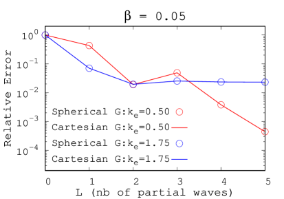
Figure 1: Relative error on $\left|\mathcal{T}_{\mathbf{k_{e}}}\right|^{2}$ in terms of the total number of partial waves of the continuum, for two values of $k_{e}$, found using either the analytical spherical (10) or cartesian (26) expression.

we plot the relative error

$$\frac{\left|\mathcal{T}_{\mathbf{k_{e}}}^{num}\right|^{2}-\left|\mathcal{T}_{\mathbf{k_{e}}}^{cG}\right|^{2}}{\left|\mathcal{T}_{\mathbf{k_{e}}}^{num}\right|^{2}}$$ (42)

in terms of the number of total partial waves, for $\beta=0.05$ and for two energies ($k_{e}=0.5$ and $1.75$ a.u.). Results obtained with the spherical and cartesian expressions yield practically the same results. Even with 6 partial terms, a relative error of $\sim 2\%$ is observed for the higher energy case. This is related to the relative quality of the representation with 30 complex Gaussians of a fast oscillating continuum, and the situation will deteriorate with increasing energy. Note that the increase of the error from $L=2$ to $L=3$ in the $k_{e}=0.5$ case is not due to the complex Gaussian representation but to a non-monotonic convergence of the partial wave expansion.

The value of the initial state Gaussian decay will regulate the radial extent of the integrand. Smaller $\beta$ values will require larger domains. The relative errors (42) are plotted in the histogram presented in Figure 2

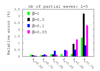
Figure 2: Relative error on $\left|\mathcal{T}_{\mathbf{k_{e}}}\right|^{2}$ in terms of the wavenumber $k_{e}$, for several initial state exponents $\beta$, computed using the analytical cartesian expression (26).

in terms of the wavenumber $k_{e}$, and for several initial state exponents $\beta=0.05,0.10,0.50,1.00$. The total number of used partial waves in this calculation is $L=5$ (6 partial waves). Here the results were obtained by using the cartesian expression (26) with (39) (again, practically indistinguishable results were found using the spherical expression (10) with (19)). They are all very good and confirm that bound to continuum transition integrals can be efficiently calculated using complex Gaussian type functions for energy values that are of physical interest.

4 Conclusions

We have studied three-dimensional multicenter integrals involving a continuum state that appear, for example, in ionization of molecules in a one-active electron picture. Through a representation in optimized complex Gaussians for the final continuum, and in real (spherical or cartesian) Gaussians for the initial bound state, we show how matrix elements for photoionization in length gauge can be calculated analytically. The result involves multiple summations. Convergence has been investigated numerically with a test case which showed that the formulation is equally efficient when using a spherical or a cartesian Gaussian description of the bound state.

This all-Gaussian approach can be formulated similarly for photoionization with the dipole operator in velocity gauge. It can also be adapted to deal with the ionization by impact of a charged particle.

Finally, we intend to go beyond the one-active electron case and tackle the more interesting, but even more challenging, two-electron integrals.

References

• [1] Jensen, F. Atomic orbital basis sets. WIREs Computational Molecular Science 2013 3, 273–295.
• [2] Shavitt, I. The Gaussian function in calculations of statistical mechanics and quantum mechanics. In: Alder, B., Fernbach, S. and Rotenberg, M., Eds., Methods in Computational Physics, Academic Press, New York 1963 1–45.
• [3] Kaufmann, K.; Baumeister, W.; Jungen, M. Universal Gaussian basis sets for an optimum representation of Rydberg and continuum wavefunctions. Journal of Physics B: Atomic, Molecular and Optical Physics 1989 22, 2223.
• [4] Nestmann, B. M.; Peyerimhoff, S. D. Optimized Gaussian basis sets for representation of continuum wavefunctions. Journal of Physics B: Atomic, Molecular and Optical Physics 1990 23, L773.
• [5] Faure, A.; Gorfinkiel, J. D.; Morgan, L. A.; Tennyson, J. GTOBAS: fitting continuum functions with Gaussian-type orbitals. Computer Physics Communications 2002 144, 224–241.
• [6] McCurdy Jr, C. W.; Rescigno, T. N. Extension of the method of complex basis functions to molecular resonances. Physical Review Letters 1978 41, 1364.
• [7] Rescigno, T. N.; McCurdy, C. W. Locally complex distortions of the energy spectrum in the calculation of scattering amplitudes and photoionization cross sections. Physical Review A 1985 31, 624.
• [8] Yu, C.; Pitzer, R. M.; McCurdy, C. W. Molecular photoionization cross sections by the complex-basis-function method. Physical Review A 1985 32, 2134.
• [9] Yabushita, S.; McCurdy, C. W.; Rescigno, T. N. Complex-basis-function treatment of photoionization in the random-phase approximation. Physical Review A 1987 36, 3146.
• [10] Morita, M.; Yabushita, S. Calculations of photoionization cross-sections with variationally optimized complex Gaussian-type basis functions. Chemical Physics 2008 349, 126–132.
• [11] Morita, M.; Yabushita, S. Photoionization cross sections of H and H2 with complex Gaussian-type basis functions optimized for the frequency-dependent polarizabilities. Journal of Computational Chemistry 2008 29, 2471–2478.
• [12] Morita, M.; Yabushita, S. Photoionization cross sections with optimized orbital exponents within the complex basis function method. Journal of Computational Chemistry 2008 29, 2317–2329.
• [13] Matsuzaki, R.; Yabushita, S. Calculation of photoionization differential cross sections using complex Gauss-type orbitals. Journal of Computational Chemistry 2017 38, 2030–2040.
• [14] Honigmann, M.; Liebermann, H. P.; Buenker, R. J. Use of complex configuration interaction calculations and the stationary principle for the description of metastable electronic states of HCl-. The Journal of Chemical Physics 2010 133, 044305.
• [15] White, A. F.; Head-Gordon, M.; McCurdy, C. W. Complex basis functions revisited: Implementation with applications to carbon tetrafluoride and aromatic N-containing heterocycles within the static-exchange approximation. The Journal of Chemical Physics 2015 142, 054103
• [16] Bubin, S.; Adamowicz, L. Computer program ATOM-MOL-nonBO for performing calculations of ground and excited states of atoms and molecules without assuming the Born-Oppenheimer approximation using all-particle complex explicitly correlated Gaussian functions. The Journal of Chemical Physics 2020 152, 204102.
• [17] Ammar, A.; Leclerc, A.; Ancarani, L. U. Fitting continuum wavefunctions with complex Gaussians: Computation of ionization cross sections. Journal of Computational Chemistry 2020 41, 2365-2377.
• [18] Ammar, A. Representation of continuum states with complex Gaussians: Application to atomic and molecular ionization processes. Ph.D. thesis. Université de Lorraine, France 2020
• [19] Ammar, A.; Ancarani, L. U.; Leclerc, A. A complex Gaussian approach to molecular photoionization. Submitted
• [20] Biedenharn, L. C.; Louck, J. D. Angular Momentum in Quantum Physics: Theory and Application. Cambridge University Press, Cambridge 1984.
• [21] Harris, F. E. Gaussian Wave functions for polyatomic molecules. Reviews of Modern Physics 1963 35, 558.
• [22] Krauss, M. Gaussian Wave Functions for Polyatomic Molecules: Integral Formulas. Journal of Research of the National Bureau of Standards: Mathematics and mathematical physics. B 1964 68, 35.
• [23] Fieck, G. Racah algebra and Talmi transformation in the theory of multi-centre integrals of Gaussian orbitals. Journal of Physics B: Atomic and Molecular Physics 1979 12, 1063.
• [24] Kaufmann, K.; Baumeister, W. Single-centre expansion of Gaussian basis functions and the angular decomposition of their overlap integrals. Journal of Physics B: Atomic, Molecular and Optical Physics 1989 22, 1.
• [25] Chiu, L. C.; Moharerrzadeh, M. Translational and rotational expansion of spherical Gaussian wave functions for multicenter molecular integrals. The Journal of Chemical Physics 1994 101, 449–458.
• [26] Moharerrzadeh, M.; Chiu, L. C. Multicenter molecular integrals of spherical Gaussian functions by Fourier transform convolution theorem. The Journal of Chemical Physics 1996 104, 616–628.
• [27] Kuang, J.; Lin, C. D. Molecular integrals over spherical Gaussian-type orbitals: I. Journal of Physics B: Atomic, Molecular and Optical Physics 1997 30, 2529.
• [28] Kuang, J.; Lin, C. D. Molecular integrals over spherical Gaussian-type orbitals: II. Modified with plane-wave phase factors. Journal of Physics B: Atomic, Molecular and Optical Physics 1997 30, 2549.
• [29] Steinborn, E. O.; Ruedenberg, K. Rotation and translation of regular and irregular solid spherical harmonics. Advances in Quantum Chemistry 1973 7, 1–81.
• [30] Abramowitz, M.; Stegun, I. A. Handbook of Mathematical Functions with Formulas, Graphs, and Mathematical Tables. Dover, New York 1972.
• [31] Niukkanen, A. W. Transformation properties of two-particle states. Chemical Physics Letters 1980 69, 174–176.
• [32] Niukkanen, A. W.; Gribov, L. A. $\Sigma$-Factorization method: A new development of molecular-orbital theories based on one-centre approximation of atomic and molecular densities. Theoretica Chimica Acta 1983 62, 443–460.
• [33] Boys, S. F. Electronic wave functions-I. A general method of calculation for the stationary states of any molecular system. Proceedings of the Royal Society of London. Series A. Mathematical and Physical Sciences 1950 200, 542–554.
• [34] Taketa, H.; Huzinaga, S.; O-ohata, K. Gaussian-expansion methods for molecular integrals. Journal of the Physical Society of Japan 1966 21, 2313–2324
• [35] Schlegel, H. B.; Frisch, M. J. Transformation between Cartesian and pure spherical harmonic Gaussians. International Journal of Quantum Chemistry 1995 54, 83–87.
• [36] Piessens, R.; de Doncker-Kapenga, E.; Überhuber, C. W.; Kahaner, D. K. QUADPACK: A subroutine package for automatic integration. Springer, New York 1983