Abstract

The Stochastic Extragradient (SEG) method is one of the most popular algorithms for solving min-max optimization and variational inequalities problems (VIP) appearing in various machine learning tasks. However, several important questions regarding the convergence properties of SEG are still open, including the sampling of stochastic gradients, mini-batching, convergence guarantees for the monotone finite-sum variational inequalities with possibly non-monotone terms, and others. To address these questions, in this paper, we develop a novel theoretical framework that allows us to analyze several variants of SEG in a unified manner. Besides standard setups, like Same-Sample SEG under Lipschitzness and monotonicity or Independent-Samples SEG under uniformly bounded variance, our approach allows us to analyze variants of SEG that were never explicitly considered in the literature before. Notably, we analyze SEG with arbitrary sampling which includes importance sampling and various mini-batching strategies as special cases. Our rates for the new variants of SEG outperform the current state-of-the-art convergence guarantees and rely on less restrictive assumptions.

1 INTRODUCTION

In the last few years, the machine learning community has been increasingly interested in differentiable game formulations where several parameterized models/players compete to minimize their respective objective functions. Notably, these formulations include generative adversarial networks (Goodfellow et al.,, 2014), proximal gradient TD learning (Liu and Wright,, 2016), actor-critic (Pfau and Vinyals,, 2016), hierarchical reinforcement learning (Wayne and Abbott,, 2014; Vezhnevets et al.,, 2017), adversarial example games (Bose et al.,, 2020), and minimax estimation of conditional moment (Dikkala et al.,, 2020).

In that context, the optimization literature has considered a slightly more general setting, namely, variational inequality problems. Given a differentiable game, its corresponding VIP designates the necessary first-order stationary optimality conditions. Under the assumption that the objectives functions of the differentiable game are convex (with respect to their respective players’ variables), the solutions of the VIP are also solutions of the original game formulation. In the unconstrained case, given an operator$F:\mathbb{R}^{d}\rightarrow\mathbb{R}^{d}$, the corresponding VIP is defined as follows:

$$\text{find }x^{*}\in\mathbb{R}^{d}\quad\text{such that}\quad F(x^{*})=0.$$ (VIP)

When the operator $F$ is monotone (a generalization of convexity), it is known that the standard gradient method does not converge without strong monotonicity (Noor,, 2003; Gidel et al.,, 2019) or cocoercivity (Chen and Rockafellar,, 1997; Loizou et al.,, 2021). Because of their convergence guarantees, even when the operator $F$ is monotone, the extragradient method (Korpelevich,, 1976) and its variants (Popov,, 1980) have been the optimization techniques of choice to solve VIP. These techniques consist of two steps: a) an extrapolation step that computes a gradient update from the current iterate, and b) an update step that updates the current iterate using the value of the vector field at the extrapolated point.

Motivated by recent applications in machine learning, in this work we are interested in cases where the objective, operator $F$, is naturally expressed as a finite sum, $F(x)=\frac{1}{n}\sum_{i=1}^{n}F_{i}(x)$ or more generally as expectation $F(x)=\mathbb{E}_{\xi}[F_{\xi}(x)].$ In that setting, we only assume to have access to a stochastic estimate of $F$.

Unfortunately, the additive value of extragradient-based techniques in the stochastic VIP setting is less apparent since the method is challenging to analyze in that setting due to the two stochastic gradient computations necessary for a single update. There are several ways to deal with the stochasticity in the SEG update. For example, one can use either independent samples (Nemirovski et al.,, 2009; Juditsky et al.,, 2011) or the same sample (Gidel et al.,, 2019) for the extrapolation and the update steps.

The selection of stepsizes in the update rule of SEG (for the extrapolation step and update step) is also a challenging task. In Chavdarova et al., (2019) it is shown that some same-stepsize variants of SEG diverge in the unconstrained monotone case. At the same time, in Hsieh et al., (2019) using a double stepsize rule, the authors provide convergence guarantees under an error-bound condition.

This discrepancy between the deterministic and the stochastic case has motivated a whole line of work (Gidel et al.,, 2019; Mishchenko et al.,, 2020; Beznosikov et al.,, 2020; Hsieh et al.,, 2019) to understand better the properties of SEG. However, several important questions remain open. To bridge this gap, in this work, we develop a novel theoretical framework that allows us to analyze several variants of SEG in a unified manner.

1.1 Preliminaries

Notation.

We use standard notation for optimization literature. We also often use $[n]$ to denote $\{1,\ldots,n\}$ and $\mathbb{E}_{\xi}[\cdot]$ for the expectation taken w.r.t. the randomness coming from $\xi$ only.

Main assumptions.

In this work, we assume that the operator $F$ is $L$-Lipschitz and $\mu$-quasi strongly monotone.

Assumption 1.1.

Operator $F(x)$ is $L$-Lipschitz, i.e., for all $x,y\in\mathbb{R}^{d}$

$$\|F(x)-F(y)\|\leq L\|x-y\|.$$ (1)

Assumption 1.2.

Operator $F(x)$ is $\mu$-quasi strongly monotone, i.e., for $\mu\geq 0$ and for all $x\in\mathbb{R}^{d}$

$$\langle F(x),x-x^{*}\rangle\geq\mu\|x-x^{*}\|^{2}.$$ (2)

We assume that $x^{*}$ is unique.

Assumption 1.1 is relatively standard and widely used in the literature on VIP. Assumption 1.2 is a relaxation of $\mu$-strong monotonicity as it includes some non-monotone games as special cases. To the best of our knowledge, the term quasi-strong monotonicity was introduced in Loizou et al., (2021) and has its roots in the quasi-strong convexity condition from the optimization literature (Necoara et al.,, 2019; Gower et al.,, 2019). In the literature of variational inequality problems, quasi strongly monotone problems are also known as strong coherent VIPs (Song et al.,, 2020) or VIPs satisfying the strong stability condition (Mertikopoulos and Zhou,, 2019). If $\mu=0$, then Assumption 1.2 is also known as variational stability condition (Hsieh et al.,, 2020; Loizou et al.,, 2021).

Variants of SEG.

In the literature of variational inequality problems there are two main stochastic extragradient variants.

The first is Same-sample SEG:

$$x^{k+1}=x^{k}-\gamma_{2,\xi^{k}}F_{\xi^{k}}\left(x^{k}-\gamma_{1,\xi^{k}}F_{\xi^{k}}(x^{k})\right),$$ (S-SEG)

where in each iteration, the same sample $\xi^{k}$ is used for the exploration (computation of $x^{k}-\gamma_{1,\xi^{k}}F_{\xi^{k}}(x^{k})$) and update (computation of $x^{k+1}$) steps. The selection of step-sizes $\gamma_{2,\xi^{k}}$ and $\gamma_{1,\xi^{k}}$ that guarantee convergence of the method in different settings varies across previous papers (Mishchenko et al.,, 2020; Beznosikov et al.,, 2020; Hsieh et al.,, 2019). In this work, the proposed stepsizes for S-SEG satisfy $0<\gamma_{2,\xi^{k}}=\alpha\gamma_{1,\xi^{k}}$, where $0<\alpha<1$, and are allowed to depend on the sample $\xi^{k}$. This specific stepsize selection is one of the main contributions of this work and we discuss its benefits in more detail in the subsequent sections.

The second variant is Independent-samples SEG

$$x^{k+1}=x^{k}-\gamma_{2}F_{\xi_{2}^{k}}\left(x^{k}-\gamma_{1}F_{\xi_{1}^{k}}(x^{k})\right),$$ (I-SEG)

where $\xi_{1}^{k},\xi_{2}^{k}$ are independent samples. Similarly to S-SEG, we assume that $0<\gamma_{2}=\alpha\gamma_{1}$, with $0<\alpha<1$, but unlike S-SEG, for I-SEG we consider stepsizes independent of samples $\xi_{1}^{k},\xi_{2}^{k}$.

Typically, S-SEG is analyzed under Lipschitzness and (strong) monotonicity of individual stochastic realizations $F_{\xi}$ (Mishchenko et al.,, 2020) that are stronger than Assumptions 1.1 and 1.2. In contrast, I-SEG is studied under Assumptions 1.1 and 1.2 but with additional assumptions like uniformly bounded variance or its relaxations (Beznosikov et al.,, 2020; Hsieh et al.,, 2020). See Appendix F.1 for further clarifications.

1.2 Contributions

Our main contributions are summarized below.

$\diamond$ Unified analysis of SEG. We develop a new theoretical framework for the analysis of SEG. In particular, we construct a unified assumption (Assumption 2.1) on the stochastic estimator, stepsizes, and the problem itself (VIP), and we prove a general convergence result under this assumption (Theorem 2.1). Next, we show that both S-SEG and I-SEG fit our theoretical framework and can be analyzed in different settings in a unified manner. In previous works, these variants of SEG have been only analyzed separately using different proof techniques. Our proposed proof technique differs significantly from those existing in the literature and, therefore, is of independent interest.

$\diamond$ Sharp rates for the known methods. Despite the generality of our framework, our convergence guarantees give tight rates for several well-known special cases. That is, the proposed analysis either recovers best-known (up to numerical factors) rates for some special cases like the deterministic EG and the I-SEG under uniformly bounded variance (UBV) assumption (Assumption 4.1 with $\delta=0$), or improves the previous SOTA results for other well known special cases, e.g., for S-SEG with uniform sampling and I-SEG under the generalized UBV assumption (Assumption 4.1 with $\delta>0$).

$\diamond$ New methods with better rates. Through our framework, we propose a general yet simple theorem describing the convergence of S-SEG under the arbitrary sampling paradigm (Gower et al.,, 2019; Loizou et al.,, 2021). Using the theoretical analysis of S-SEG with arbitrary sampling, we can provide tight convergence guarantees for several well-known methods like the deterministic/full-batch EG and S-SEG with uniform sampling (S-SEG-US) as well as some variants of S-SEG that were never explicitly considered in the literature before. For example, we are first to analyze S-SEG with mini-batch sampling without replacement ($b$-nice sampling; S-SEG-NICE) and show its theoretical superiority to vanilla S-SEG-US. Moreover, we propose a new method called S-SEG-IS that combines S-SEG with importance sampling – the sampling strategy, when the $i$-th operator from the sum is chosen with probability proportional to its Lipschitz constant. We prove the theoretical superiority of S-SEG-IS in comparison to S-SEG-US.

$\diamond$ Novel stepsize selection. One of the key ingredients of our approach is the use of sample-dependent stepsizes. This choice of stepsizes is especially important for the S-SEG-IS, as it allows us to obtain better theoretical guarantees compared to the S-SEG-US. Moreover, as in Hsieh et al., (2020), for the update step we also use smaller stepsizes than for the exploration step: $\gamma_{2,\xi^{k}}\leq\gamma_{1,\xi^{k}}$ ($\gamma_{2}\leq\gamma_{1}$). However, unlike the results by Hsieh et al., (2020), our theory allows using $\gamma_{2,\xi^{k}}=\alpha\gamma_{1,\xi^{k}}$ with constant parameter $\alpha<1$ to achieve any predefined accuracy of the solution.

$\diamond$ Convergence guarantees under weak conditions. The flexibility of our approach helps us to derive our main theoretical results under weak assumptions. In particular, in the analysis of S-SEG, we allow the stochastic realizations $F_{\xi}$ to be $(\mu_{\xi},x^{*})$-quasi strongly monotone with possibly negative $\mu_{\xi}$, meaning that $F_{\xi}$ can be non-monotone (see Assumption 3.2). In addition, in the analysis of S-SEG we do not require any bounded variance assumption. To the best of our knowledge, all previous works on the analysis of S-SEG require monotonicity of $F_{\xi}$. Finally, in the analysis of I-SEG we obtain last-iterate convergence guarantees by only assuming $\mu$-quasi strong monotonicity of $F$, which, as we explained before, is satisfied for some classes of non-monotone problems.

$\diamond$ Numerical evaluation. In Section 5, we corroborate our theoretical results with experimental testing.

Table 1: Summary of the state-of-the-art convergence result for S-SEG and I-SEG. Our results are highlighted in green. Columns with convergence rates provide the upper bounds for $\mathbb{E}[\|x^{K}-x^{*}\|^{2}]$. Numerical constants are omitted. Notation: $\mu_{\min}=\min_{i\in[n]}\mu_{i}$; $\overline{\mu}=\frac{1}{n}\sum_{i\in[n]:\mu_{i}\geq 0}\mu_{i}+\frac{4}{n}\sum_{i\in[n]:\mu_{i}<0}\mu_{i}$; $L_{\max}=\max_{i\in[n]}L_{i}$; $\overline{L}=\frac{1}{n}\sum_{i=1}^{n}L_{i}$ (can be much smaller than $L_{\max}$); $R_{0}^{2}=\|x^{0}-x^{*}\|^{2}$; $\sigma_{{\sf US}*}^{2}=\frac{1}{n}\sum_{i=1}^{n}\|F_{i}(x^{*})\|^{2}$; $\sigma_{{\sf IS}*}^{2}=\frac{1}{n}\sum_{i=1}^{n}\frac{\overline{L}}{L_{i}}\|F_{i}(x^{*})\|^{2}$ (can be much smaller than $\sigma_{{\sf US}*}^{2}$); $\delta$ and $\sigma^{2}$ = parameters from As. 4.1; $b=$ batchsize. Assumptions on constant stepsizes: Mishchenko et al., (2020) uses $\gamma\leq\nicefrac{{1}}{{2L_{\max}}}$, Hsieh et al., (2019) uses $\gamma_{2}\leq\gamma_{1}\leq\nicefrac{{c}}{{L}}$ for some positive $c>0$, Beznosikov et al., (2020) uses $\gamma\leq\nicefrac{{1}}{{4L}}$, and we use $\gamma_{1,\xi}=\gamma\leq\nicefrac{{1}}{{6L_{\max}}}$ for S-SEG-US, $\gamma_{1,\xi}=\nicefrac{{\gamma\overline{L}}}{{L_{\xi}}},\gamma\leq\nicefrac{{1}}{{6\overline{L}}}$ for S-SEG-IS, $\gamma_{1,\xi}=\gamma\leq\min\left\{\frac{\mu b}{18\delta},\frac{1}{4\mu+\sqrt{6(L^{2}+\nicefrac{{\delta}}{{b}})}}\right\}$ for I-SEG, and in all cases $\gamma_{2,\xi}=\alpha\gamma_{1}$ with $\alpha<1$. Numerical factors in our theoretical estimates can be tightened for S-SEG when $\mu_{i}\geq 0$ and for I-SEG when $\delta=0$.

Setup	Method	Citation	Convergence Rate for
			Constant Stepsize	Diminishing Stepsize
$F(x)=\frac{1}{n}\sum\limits_{i=1}^{n}F_{i}(x)$ + As. 3.1, 3.2	S-SEG-US	(Mishchenko et al.,, 2020)(1)	$(1-\gamma\mu_{\min})^{K}R_{0}^{2}+\frac{\gamma\sigma_{{\sf US*}}^{2}}{\mu_{\min}}$	$\frac{L_{\max}R_{0}^{2}}{\mu_{\min}}\exp\left(-\frac{\mu_{\min}K}{L_{\max}}\right)+\frac{\sigma_{{\sf US*}}^{2}}{\mu_{\min}^{2}K}$(2)
		This paper	$(1-\gamma\overline{\mu})^{K}R_{0}^{2}+\frac{\gamma\sigma_{{\sf US*}}^{2}}{\overline{\mu}}$	$\frac{L_{\max}R_{0}^{2}}{\overline{\mu}}\exp\left(-\frac{\overline{\mu}K}{L_{\max}}\right)+\frac{\sigma_{{\sf US*}}^{2}}{\overline{\mu}^{2}K}$
	S-SEG-IS	This paper	$(1-\gamma\overline{\mu})^{K}R_{0}^{2}+\frac{\gamma\sigma_{{\sf IS*}}^{2}}{\overline{\mu}}$	$\frac{\overline{L}R_{0}^{2}}{\overline{\mu}}\exp\left(-\frac{\overline{\mu}K}{\overline{L}}\right)+\frac{\sigma_{{\sf IS*}}^{2}}{\overline{\mu}^{2}K}$
$F(x)=\mathbb{E}_{\xi}[F_{\xi}(x)]$ + As. 1.1, 1.2, 4.1	I-SEG	(Hsieh et al.,, 2020)(3)	$(1-\gamma_{1}\gamma_{2}\mu^{2})^{K}R_{0}^{2}+\frac{C\sigma^{2}}{\mu^{2}b}$ $C=\gamma_{1}L(1+\gamma_{1}L)+\frac{\gamma_{2}}{\gamma_{1}}$	$\frac{L^{2}\sigma^{2}}{\mu^{4}bK^{\nicefrac{{1}}{{3}}}}$(4)
		(Beznosikov et al.,, 2020)(5)	$(1-\gamma\mu)^{K}R_{0}^{2}+\frac{\gamma\sigma^{2}}{\mu b}$	$R_{0}^{2}\exp\left(-\frac{\mu K}{L}\right)+\frac{\sigma^{2}}{\mu^{2}bK}$(6)
		This paper	$(1-\gamma\mu)^{K}R_{0}^{2}+\frac{\gamma\sigma^{2}}{\mu b}$	$\kappa R_{0}^{2}\exp\left(-\frac{K}{\kappa}\right)+\frac{\sigma^{2}}{\mu^{2}bK}$ $\kappa=\max\left\{\frac{\delta}{\mu^{2}b},\frac{L+\sqrt{\nicefrac{{\delta}}{{b}}}}{\mu}\right\}$

• Mishchenko et al., (2020) consider a regularized version of (VIP) with $\mu_{\min}$-strongly convex regularization, $F(x)=\mathbb{E}_{\xi}[F_{\xi}(x)]$ and $F_{\xi}(x)$ being monotone and $L_{\xi}$-Lipschitz. In this case, one can construct an equivalent problem with convex regularizer, $F(x)=\mathbb{E}_{\xi}[F_{\xi}(x)]$ and $F_{\xi}(x)$ being $\mu_{\min}$-strongly monotone and $L_{\xi}$-Lipschitz. If regularization is zero in the obtained problem and $\mathbb{E}_{\xi}[F_{\xi}(x)]=\frac{1}{n}\sum_{i=1}^{n}F_{i}(x)$, the problem from (Mishchenko et al.,, 2020) fits the considered setup with $\mu_{i}>0$ for all $i\in[n]$.

• Mishchenko et al., (2020) do not consider diminishing stepsizes, but this rate can be derived from their Theorem 2 using similar steps as we use for our results.

• Hsieh et al., (2020) consider As. 4.1, but do not provide explicit rates when $\delta>0$. Moreover, instead of $\mu$-quasi strong monotonicity they use slightly different assumption: $\|F(x)\|\geq\mu\|x-x^{*}\|$.

• This bound holds only for large enough $K$ and $\sigma>0$. Factor $\nicefrac{{L^{2}}}{{\mu^{4}}}$ is not explicitly given in (Hsieh et al.,, 2020). We derive this rate using $\gamma_{1,k}=\nicefrac{{\gamma_{1}}}{{(k+t)^{\nicefrac{{2}}{{3}}}}}$, $\gamma_{2,k}=\nicefrac{{\gamma_{2}}}{{(k+t)^{\nicefrac{{1}}{{3}}}}}$ with largest possible $\gamma_{1}\sim\nicefrac{{1}}{{\mu}}$, $\gamma_{2}\sim\nicefrac{{1}}{{\mu}}$ and smallest possible $t\sim(\nicefrac{{L}}{{\mu}})^{3}$ for given $\gamma_{1}$ and $\gamma_{2}$.

• Results are derived for the case $\delta=0$. Beznosikov et al., (2020) study a distributed version of I-SEG.

• This result is derived for the stepsize $\gamma$ that explicitly depends on $K$ and $\sigma^{2}$, which makes it hard to use this stepsize in practice.

1.3 Related Work

Non-monotone VIP with special structure.

Recent works of Daskalakis et al., (2021) and Diakonikolas et al., (2021) show that, for general non-monotone VIP, the computation of approximate first-order locally optimal solutions is intractable, motivating the identification of structural assumptions on the objective function for which these intractability barriers can be bypassed.

In this work, we focus on such settings (structured non-monotone operators) for which we are able to provide tight convergence guarantees and avoid the standard issues (like cycling and divergence of the methods) appearing in the more general non-monotone regime. In particular, we focus on quasi-strongly monotone VIPs (2). Recently, similar conditions have been used in several papers to provide convergence guarantees of algorithms for solving such structured classes of non-monotone problems. For example,Yang et al., (2020) focuses on analyzing alternating gradient descent ascent under the Two-sided Polyak- Lojasiewicz inequality, while Hsieh et al., (2020) provides convergence guarantees of double stepsize stochastic extragradient for problems satisfying the error bound condition. Song et al., (2020) and Loizou et al., (2021) study the optimistic dual extrapolation and the stochastic gradient descent-ascent and stochastic consensus optimization method, respectively, for solving quasi-strongly monotone problems. Kannan and Shanbhag, (2019) provides an analysis for the stochastic extragradient for the class of strongly pseudo-monotone VIPs. The convergence of Hamiltonian methods for solving (stochastic) sufficiently bilinear games (class of structured non-monotone games) was studied in Abernethy et al., (2021) and Loizou et al., (2020).

On the analysis of stochastic extragradient.

In the context of VIP, SEG is also known as Stochastic Mirror Prox Juditsky et al., (2011). Several novel variants of SEG have been proposed and analyzed in recent papers, such as accelerated versions (Chen et al.,, 2017), single-call variants (a.k.a. optimistic methods) Hsieh et al., (2019), and a version with player sampling in the context of multi-player games (Jelassi et al.,, 2020). Comparing our results with these variants is outside of the scope of this paper. In this work, we focus on analyzing and better understanding the properties of the standard version of SEG with independent (I-SEG) or same sample (S-SEG).

Recent analysis of SEG by Mishchenko et al., (2020), Hsieh et al., (2020) and Beznosikov et al., (2020) have extended the seminal results of Juditsky et al., (2011) in the unconstrained case. We compare their results with our work in Table 1.

SEG has also been analyzed in settings that significantly differ from ours such as in the constrained pseudomonotone case (Kannan and Shanbhag,, 2019) and the unconstrained bilinear case (Li et al.,, 2021).

Arbitrary sampling paradigm.

The first analysis of a stochastic optimization algorithm with an arbitrary sampling was performed by Richtárik and Takáč, (2016) in the context of randomized coordinate descent method for strongly convex functions. This arbitrary sampling paradigm was later extended in different settings, including accelerated coordinate descent for (strongly) convex functions (Hanzely and Richtárik,, 2019; Qu and Richtárik,, 2016), randomized iterative methods for solving linear systems (Richtárik and Takác,, 2020; Loizou and Richtárik, 2020b, ; Loizou and Richtárik, 2020a, ), randomized gossip algorithms (Loizou and Richtárik,, 2021), variance-reduced methods with convex (Khaled et al.,, 2020), and nonconvex (Horváth and Richtárik,, 2019) objectives. The first analysis of SGD under the arbitrary sampling was proposed in Gower et al., (2019) for (quasi)-strongly convex problems and later extended to the non-convex regime in Gower et al., (2021) and Khaled and Richtárik, (2020). In the area of smooth games and variational inequality problems the first papers that provide an analysis of stochastic algorithms under the arbitrary sampling paradigm are (Loizou et al.,, 2020, 2021). In Loizou et al., (2020, 2021), the authors focus on algorithms like the stochastic Hamiltonian method, the stochastic gradient descent ascent, and the stochastic consensus optimization. To the best of our knowledge, our work is the first that provides an analysis of SEG under the arbitrary sampling paradigm.

1.4 Paper Organization

Section 2 introduces our unified theoretical framework that is applied for the analysis of S-SEG and I-SEG in Sections 3 and 4 respectively. In section 5, we report the result of our numerical experiments, and we make the concluding remarks in Section 6. Proofs, technical details, and additional experiments are given in Appendix. We defer the discussion of our results for quasi monotone ($\mu=0$) problems to Appendix B.

2 GENERAL ANALYSIS OF SEG

To analyze the convergence of SEG, we consider a family of methods

$$x^{k+1}=x^{k}-\gamma_{\xi^{k}}g_{\xi^{k}}(x^{k}),$$ (3)

where $g_{\xi^{k}}(x^{k})$ is some stochastic operator evaluated at point $x^{k}$ and $\xi^{k}$ encodes the randomness/stochasticity appearing at iteration $k$ (e.g., it can be the sample used at step $k$). Parameter $\gamma_{\xi^{k}}$ is the stepsize that is allowed to depend on $\xi^{k}$. Inspired by Gorbunov et al., (2020), let us introduce the following general assumption on operator $g_{\xi^{k}}(x^{k})$, stepsize $\gamma_{\xi^{k}}$, and the problem (VIP).

Assumption 2.1.

We assume that there exist non-negative constants $A,B,C,D_{1},D_{2}\geq 0$, $\rho\in[0,1]$, and (possibly random) non-negative sequence $\{G_{k}\}_{k\geq 0}$ such that

$$\mathbb{E}_{\xi^{k}}\left[\gamma_{\xi^{k}}^{2}\|g_{\xi^{k}}(x^{k})\|^{2}\right]\leq 2AP_{k}+C\|x^{k}-x^{*}\|^{2}+D_{1},$$ (4)

$$P_{k}\geq\rho\|x^{k}-x^{*}\|^{2}+BG_{k}-D_{2},$$ (5)

where $P_{k}=\mathbb{E}_{\xi^{k}}\left[\gamma_{\xi^{k}}\langle g_{\xi^{k}}(x^{k}),x^{k}-x^{*}\rangle\right]$.

Although inequalities (4) and (5) may seem unnatural, they are satisfied with certain parameters for several variants of S-SEG and I-SEG under reasonable assumptions on the problem and the stochastic noise. Moreover, these inequalities have a simple intuition behind them. That is, inequality (4) is a generalization of the expected cocoercivity introduced in Loizou et al., (2021), adjusted to the case of biased estimators $g_{\xi^{k}}(x^{k})$ of $F(x^{k})$, as it is the case for SEG. The biasedness of $g_{\xi^{k}}(x^{k})$ and the (possible) dependence of $\gamma_{\xi^{k}}$ on $\xi^{k}$ force us to introduce the expected inner product $P_{k}=\mathbb{E}_{\xi^{k}}\left[\gamma_{\xi^{k}}\langle g_{\xi^{k}}(x^{k}),x^{k}-x^{*}\rangle\right]$ instead of using $P_{k}\sim\langle F(x^{k}),x^{k}-x^{*}\rangle$ as in Loizou et al., (2021). Moreover, unlike the expected cocoercivity, our assumption (4) does not imply (star-)cocoercivity of $F$. However, when we derive (4) for S-SEG and I-SEG we rely in Lipschitzness of $F$ or its stochastic realizations. The terms $C\|x^{k}-x^{*}\|^{2}$ and $D_{1}$ characterize the noise structure, and $A$ is typically some constant smaller than $\nicefrac{{1}}{{2}}$.

Next, inequality (5) can be seen as a modification of $\mu$-quasi strong monotonicity of $F$ (2). Indeed, if we had $\gamma_{\xi^{k}}=\gamma$ and $\mathbb{E}_{\xi^{k}}[g_{\xi^{k}}(x^{k})]=F(x^{k})$, then we would have $P_{k}=\gamma\langle F(x^{k}),x^{k}-x^{*}\rangle$ and inequality (5) would have been satisfied with $\rho=\gamma\mu$, $B=0$, $G_{k}=0$, $D_{2}=0$ for $F$ being $\mu$-quasi strongly monotone. However, because of the biasedness of $g_{\xi^{k}}(x^{k})$ we have to account to the noise encoded by $D_{2}$. In inequality (5), $\rho$ also typically depends on some quantity related to the quasi-strong monotonicity and the stepsize. Moreover, when $g_{\xi^{k}}(x^{k})$ corresponds to SEG, we are able to show that $B>0$ with $G_{k}$ being an upper bound for $\|F(x^{k})\|^{2}$ up to the factors depending on the stepsize selection (see Sections  3 and 4).

Under this assumption, we derive the following result.

Theorem 2.1.

Let Assumption 2.1 hold with $A\leq\nicefrac{{1}}{{2}}$ and $\rho>C\geq 0$. Then, the iterates of SEG given by (3) satisfy

$$\mathbb{E}\left[\|x^{K}-x^{*}\|^{2}\right]\leq(1+C-\rho)^{K}\|x^{0}-x^{*}\|^{2}+\frac{D_{1}+D_{2}}{\rho-C}.$$

In the case that Assumption 2.1 holds with $\rho=C=0$, $B>0$, then for all $K\geq 0$, the iterates of SEG given by (3) satisfy

$$\frac{1}{K+1}\sum\limits_{k=0}^{K}\mathbb{E}[G_{k}]\leq\frac{\|x^{0}-x^{*}\|^{2}}{B(K+1)}+\frac{D_{1}+D_{2}}{B}.$$

This theorem establishes linear convergence rate when $\rho>C\geq 0$ and ${\cal O}(\nicefrac{{1}}{{K}})$ rate when $\rho=C=0$, $B>0$ to a neighborhood of the solution with the size proportional to the noise parameters $D_{1},D_{2}$. In all special cases that we consider, the first case corresponds to the quasi-strongly monotone problems and the second one – to quasi-monotone problems. All the rates from this paper are derived via Theorem 2.1.

3 SAME-SAMPLE SEG (S-SEG)

Consider the situation when we have access to Lipschitz-continuous stochastic realization $F_{\xi}(x)$ and can compute $F_{\xi}$ at different points for the same $\xi$. For such problems, we consider S-SEG.

3.1 Arbitrary Sampling

Below we introduce reasonable assumptions on the stochastic trajectories that cover a wide range of sampling strategies. Therefore, following Gower et al., (2019); Loizou et al., (2021), we use the name arbitrary sampling to define this setup. First, we assume Lischitzness of $F_{\xi}$.

Assumption 3.1.

We assume that for all $\xi$ there exists $L_{\xi}>0$ such that operator $F_{\xi}(x)$ is $L_{\xi}$-Lipschitz, i.e., for all $x\in\mathbb{R}^{d}$

$$\|F_{\xi}(x)-F_{\xi}(y)\|\leq L_{\xi}\|x-y\|.$$ (6)

The next assumption can be considered as a relaxation of standard strong monotonicity allowing $F_{\xi}(x)$ to be non-monotone with a certain structure.

Assumption 3.2.

We assume that for all $\xi$ operator $F_{\xi}(x)$ is $(\mu_{\xi},x^{*})$-strongly monotone, i.e., there exists (possibly negative) $\mu_{\xi}\in\mathbb{R}$ such that for all $x\in\mathbb{R}^{d}$

$$\langle F_{\xi}(x)-F_{\xi}(x^{*}),x-x^{*}\rangle\geq\mu_{\xi}\|x-x^{*}\|^{2}.$$ (7)

We emphasize that some $\mu_{\xi}$ are allowed to be arbitrary heterogeneous and even negative, which allows to have non-monotone $F_{\xi}$. Moreover, if $F_{\xi}$ is $L_{\xi}$-Lipschitz, then in view of Cauchy-Schwarz inequality, (7) holds with $-L_{\xi}\leq\mu_{\xi}\leq L_{\xi}$. Indeed, inequality (6) implies $-L_{\xi}\|x-x^{*}\|^{2}\leq-\|F_{\xi}(x)-F_{\xi}(x^{*})\|\cdot\|x-x^{*}\|\leq\langle F_{\xi}(x)-F_{\xi}(x^{*}),x-x^{*}\rangle\leq\|F_{\xi}(x)-F_{\xi}(x^{*})\|\cdot\|x-x^{*}\|\leq L_{\xi}\|x-x^{*}\|^{2}$. However, $\mu_{\xi}$ can be much larger than $-L_{\xi}$. When $F_{\xi}(x^{*})=0$ and $\mu_{\xi}\geq 0$, inequality (7) recovers quasi-strong monotonicity of $F_{\xi}$, i.e., $F_{\xi}$ can be non-monotone even when $\mu_{\xi}\geq 0$.

Finally, we assume that the following two conditions are satisfied:

$$\mathbb{E}_{\xi^{k}}[\gamma_{1,\xi^{k}}F_{\xi^{k}}(x^{*})] = 0,$$ (8)

$$\mathbb{E}_{\xi^{k}}[\gamma_{1,\xi^{k}}\mu_{\xi^{k}}(\mathds{1}_{\{\mu_{\xi^{k}}\geq 0\}}+4\cdot\mathds{1}_{\{\mu_{\xi^{k}}<0\}})] \geq 0,$$ (9)

where $\mathds{1}_{\texttt{condition}}=1$ if condition holds, and $\mathds{1}_{\texttt{condition}}=0$ otherwise. Here, (8) is a generalization of unbiasedness at $x^{*}$, since $F(x^{*})=0$, and the left-hand side of (9) is a generalization of the averaged quasi-strong monotonicity constant multiplied by the stepsize. Moreover, (9) holds when all $\mu_{\xi}\geq 0$, which is typically assumed in the analysis of S-SEG. The numerical constant $4$ in (9) appears mainly due to the technical reasons coming from our proof technique.

To better illustrate the generality of conditions (8)-(9), let us provide three different examples where these conditions are satisfied. In all examples, we assume that $F(x)=\frac{1}{n}\sum_{i=1}^{n}F_{i}(x)$ and $F_{i}(x)$ is $(\mu_{i},x^{*})$-strongly monotone and $L_{i}$-Lipschitz.

Let us start by considering the standard single-element uniform sampling strategy.

Example 3.1 (Uniform sampling).

Let $\xi^{k}$ be sampled from the uniform distribution on $[n]$, i.e., for all $i\in[n]$ we have $\mathbb{P}\left[\xi^{k}=i\right]=p_{i}\equiv\nicefrac{{1}}{{n}}$. If

$$\overline{\mu}=\frac{1}{n}\sum\limits_{i:\mu_{i}\geq 0}\mu_{i}+\frac{4}{n}\sum\limits_{i:\mu_{i}<0}\mu_{i}\geq 0$$ (10)

and $\gamma_{1,\xi}\equiv\gamma>0$, then conditions (8)-(9) hold.

In the above example, the oracle is unbiased and, as the result, we use constant stepsize $\gamma_{1,\xi}=\gamma$. Next, we note that $\overline{\mu}$ satisfies: $\mu\geq\overline{\mu}\geq\mu_{\min}$, where $\mu$ is the parameter from (2), and $\mu_{\min}=\min_{i\in[n]}\mu_{i}$. Moreover, we emphasize that to fulfill conditions (8)-(9) in Example 3.1, and in the following examples we only need to assume that parameter $\gamma$ is positive. However, to be able to derive convergence guarantees for S-SEG under different sampling strategies we will later introduce an additional upper bound for $\gamma$ (see Section 3.2).

Next, we consider a uniform sampling strategy of mini-batching without replacement.

Example 3.2 ($b$-nice sampling).

Let $\xi$ be a random subset of size $b\in[n]$ chosen from the uniform distribution on the family of all $b$-elements subsets of $[n]$. Next, let $F_{\xi}(x)=\frac{1}{b}\sum_{i\in\xi}F_{i}(x)$. If

$$\overline{\mu}_{b-{\sf NICE}}=\frac{1}{\binom{n}{b}}\left(\sum\limits_{\overset{S\subseteq[n],}{|S|=b:\mu_{S}\geq 0}}\!\mu_{S}+4\sum\limits_{\overset{S\subseteq[n],}{|S|=b:\mu_{S}<0}}\!\mu_{S}\right)\geq 0,$$

where $\mu_{S}\geq\frac{1}{b}\sum_{i\in S}\mu_{i}$ is such that the operator $\frac{1}{b}\sum_{i\in S}F_{i}(x)$ is $(\mu_{S},x^{*})$-strongly monotone, and $\gamma_{1,\xi}\equiv\gamma>0$, then conditions (8)-(9) hold.

Finally, we provide an example of a non-uniform sampling.

Example 3.3 (Importance sampling).

Let $\xi^{k}$ be sampled from the following distribution: for $i\in[n]$

$$\mathbb{P}\left[\xi^{k}=i\right]=p_{i}=\frac{L_{i}}{\sum\limits_{j=1}^{n}L_{j}}.$$ (11)

If (10) is satisfied and $\gamma_{1,\xi}=\nicefrac{{\gamma\overline{L}}}{{L_{\xi}}}$, where $\overline{L}=\frac{1}{n}\sum_{i=1}^{n}L_{i}$, $\gamma>0$, then conditions (8)-(9) hold.

We provide rigorous proofs that the above examples, as well as additional ones, fit the conditions (8)-(9) in Appendix E.1.

3.2 Convergence of S-SEG

Having explained the main sampling strategies of S-SEG that we are focusing on this work, let us now present our main convergence analysis results for this method.

Let assumptions 3.1 and 3.2 hold, and let us select the stepsize $\gamma_{1,\xi^{k}}$ such that conditions (8)-(9) are satisfied, and

$$\gamma_{1,\xi^{k}}\leq\frac{1}{4|\mu_{\xi^{k}}|+\sqrt{2}L_{\xi^{k}}}.$$ (12)

Then one is able to show that Assumption 2.1 is satisfied (see Appendix E.2 for this derivation) for $g_{\xi^{k}}(x^{k})=F_{\xi^{k}}\left(x^{k}-\gamma_{1,\xi^{k}}F_{\xi^{k}}(x^{k})\right)$ and $\gamma_{\xi^{k}}=\gamma_{2,\xi^{k}}$. In particular, under these conditions, Assumption 2.1 holds with $A=2\alpha$, $C=0$, $B=\nicefrac{{1}}{{2}}$, $D_{1}=6\alpha^{2}\sigma_{{\sf AS}}^{2}$, $D_{2}=\nicefrac{{3\alpha\sigma_{{\sf AS}}^{2}}}{{2}}$, and

$$\sigma_{{\sf AS}}^{2}=\mathbb{E}_{\xi}\left[\gamma_{1,\xi}^{2}\|F_{\xi}(x^{*})\|^{2}\right],$$ (13)

$$\rho=\frac{\alpha}{2}\mathbb{E}_{\xi^{k}}[\gamma_{1,\xi^{k}}\mu_{\xi^{k}}(\mathds{1}_{\{\mu_{\xi^{k}}\geq 0\}}+4\cdot\mathds{1}_{\{\mu_{\xi^{k}}<0\}})],$$ (14)

$$G_{k}=\alpha\mathbb{E}_{\xi^{k}}\left[\gamma_{1,\xi^{k}}^{2}\widehat{B}_{\xi^{k}}\|F_{\xi^{k}}(x^{k})\|^{2}\right],$$ (15)

where $\widehat{B}_{\xi^{k}}=1-4|\mu_{\xi^{k}}|\gamma_{1,\xi^{k}}-2L_{\xi^{k}}^{2}\gamma_{1,\xi^{k}}^{2}$. Here (12) implies that $\widehat{B}_{\xi^{k}}\geq 0$. Therefore, applying our general result (Theorem 2.1), we derive the following convergence guarantees for S-SEG.

Theorem 3.1.

Let Assumptions 3.2 and 3.1 hold. If $\gamma_{2,\xi^{k}}=\alpha\gamma_{1,\xi_{k}}$, $0<\alpha\leq\nicefrac{{1}}{{4}}$, and $\gamma_{1,\xi^{k}}$ satisfies (8)-(9) and (12) and $\rho$ from (14) is positive, then the iterates of S-SEG satisfy

$$\mathbb{E}\left[\|x^{K}-x^{*}\|^{2}\right]\!\leq\!\left(1\!-\!\rho\right)^{K}\!\|x^{0}-x^{*}\|^{2}+\frac{3\alpha\left(4\alpha\!+\!1\right)\sigma_{{\sf AS}}^{2}}{2\rho},$$

where $\sigma_{{\sf AS}}^{2}$ is defined in (14).

The next corollary establishes the convergence rate with diminishing stepsizes allowing to reduce the size of the neighborhood.

Corollary 3.1.

Let Assumptions 3.2 and 3.1 hold, and let $\gamma_{2,\xi^{k}}=\alpha\gamma_{1,\xi_{k}}$ with $\alpha=\nicefrac{{1}}{{4}}$, and $\gamma_{1,\xi^{k}}=\beta_{k}\cdot\gamma_{\xi^{k}}$, where $\gamma_{\xi^{k}}$ satisfies (8), (9), (12), and $\widetilde{\rho}=\frac{1}{8}\mathbb{E}_{\xi^{k}}[\gamma_{\xi^{k}}\mu_{\xi^{k}}(\mathds{1}_{\{\mu_{\xi^{k}}\geq 0\}}+4\cdot\mathds{1}_{\{\mu_{\xi^{k}}<0\}})]$. Assume that $\widetilde{\rho}>0$. Then, for all $K\geq 0$ and $\{\beta_{k}\}_{k\geq 0}$ such that

$$\text{if }K\leq\frac{1}{\widetilde{\rho}}, \beta_{k}=1,$$

$$\text{if }K>\frac{1}{\widetilde{\rho}}\text{ and }k<k_{0}, \beta_{k}=1,$$ (16)

$$\text{if }K>\frac{1}{\widetilde{\rho}}\text{ and }k\geq k_{0}, \beta_{k}=\frac{2}{2+\widetilde{\rho}(k-k_{0})},$$

where $k_{0}=\left\lceil\nicefrac{{K}}{{2}}\right\rceil$, we have that the iterates of S-SEG satisfy

$$\mathbb{E}\left[\|x^{K}-x^{*}\|^{2}\right]\!\leq\!\frac{32\|x^{0}\!-\!x^{*}\|^{2}}{\widetilde{\rho}}\exp\left(-\frac{\widetilde{\rho}K}{2}\right)+\frac{27\sigma_{{\sf AS}}^{2}}{\widetilde{\rho}^{2}K}.$$

We notice that the stepsize schedule from the above corollary requires the knowledge of the total number of iterations $K$.

Next, we provide the results for the special cases described in Section 3.1. These results are direct corollaries of Theorem 3.1 and Corollary 3.1.

S-SEG-US: S-SEG with Uniform Sampling.

Consider the setup from Example 3.1. Then, Theorem 3.1 implies that for constant stepsizes $\gamma_{1,\xi^{k}}$ and $\gamma_{2,\xi^{k}}$, the iterates of S-SEG-US satisfy

$$\mathbb{E}\left[\|x^{K}-x^{*}\|^{2}\right] \leq \left(1-\frac{\alpha\gamma\overline{\mu}}{2}\right)^{K}\|x^{0}-x^{*}\|^{2}$$

$$\quad+\frac{3\left(4\alpha+1\right)\gamma\sigma_{{\sf US*}}^{2}}{\overline{\mu}},$$

where $\gamma\leq\nicefrac{{1}}{{6L_{\max}}}$, $L_{\max}=\max_{i\in[n]}L_{i}$, and $\sigma_{{\sf US*}}^{2}=\frac{1}{n}\sum\limits_{i=1}^{n}\|F_{i}(x^{*})\|^{2}$. For diminishing stepsizes following (16), Corollary 3.1 implies that for the iterates of S-SEG-US $\mathbb{E}\left[\|x^{K}-x^{*}\|^{2}\right]$ is of the order

$${\cal O}\left(\frac{L_{\max}R_{0}^{2}}{\overline{\mu}}\exp\left(-\frac{\overline{\mu}K}{L_{\max}}\right)+\frac{\sigma_{{\sf US*}}^{2}}{\overline{\mu}^{2}K}\right),$$

where $R_{0}=\|x^{0}-x^{*}\|^{2}$. The previous SOTA rate for S-SEG-US (Mishchenko et al.,, 2020) assumes that $\mu_{i}>0$ for all $i\in[n]$ and depends on $\mu_{\min}=\min_{i\in[n]}\mu_{i}$ which can be much smaller than $\overline{\mu}$. That is, our results for S-SEG-US are derived under weaker assumptions and are tighter than the previous ones for this method.

S-SEG-NICE: S-SEG with $b$-Nice Sampling.

Consider the setup from Example 3.2. Then, Theorem 3.1 implies that for constant stepsizes $\gamma_{1,\xi^{k}}$ and $\gamma_{2,\xi^{k}}$, the iterates of S-SEG-NICE satisfy

$$\mathbb{E}\left[\|x^{K}-x^{*}\|^{2}\right] \leq \left(1-\frac{\alpha\gamma\overline{\mu}_{b-{\sf NICE}}}{2}\right)^{K}\|x^{0}-x^{*}\|^{2}$$

$$\quad+\frac{3\left(4\alpha+1\right)\gamma\sigma_{b-{\sf NICE*}}^{2}}{\overline{\mu}_{b-{\sf NICE}}},$$

where $\gamma\leq\nicefrac{{1}}{{6L_{b-{\sf NICE}}}}$, $L_{b-{\sf NICE}}=\max_{S\subseteq[n],|S|=b}L_{S}$, and $\sigma_{b-{\sf NICE*}}^{2}=\frac{n-b}{b(n-1)}\sigma_{{\sf US}*}$. For diminishing stepsizes following (16), Corollary 3.1 implies that for the iterates of S-SEG-NICE $\mathbb{E}\left[\|x^{K}-x^{*}\|^{2}\right]$ is of the order

$${\cal O}\left(\frac{L_{b-{\sf NICE}}R_{0}^{2}}{\overline{\mu}_{b-{\sf NICE}}}\exp\left(-\frac{\overline{\mu}_{b-{\sf NICE}}K}{L_{b-{\sf NICE}}}\right)+\frac{\sigma_{b-{\sf NICE*}}^{2}}{\overline{\mu}_{b-{\sf NICE}}^{2}K}\right).$$

These rates show the benefits of mini-batching without replacement: the linearly decaying term decreases faster than the corresponding one for S-SEG-US since $L_{b-{\sf NICE}}\leq L_{\max}$ and $\overline{\mu}_{b-{\sf NICE}}\geq\overline{\mu}$, and the variance $\sigma_{b-{\sf NICE*}}^{2}$ is smaller than $\sigma_{{\sf US}*}^{2}$, i.e., ${\cal O}(1/K)$ term for S-SEG-NICE is more than $b$-times smaller than the corresponding term for S-SEG-US.

Moreover, we highlight that for $n=b$ we recover the rate of deterministic EG up to numerical factors. That is, for the deterministic EG we obtain $\|x^{K}-x^{*}\|^{2}\leq\left(1-\nicefrac{{\alpha\gamma\mu}}{{2}}\right)^{K}\|x^{0}-x^{*}\|^{2}$ with $\gamma\leq\nicefrac{{1}}{{6L}}$, since $\overline{\mu}_{b-{\sf NICE}}=\mu$ and $L_{b-{\sf NICE}}=L$ in this case. This fact highlights the tightness of our analysis, since in the known special cases our general theorem either recovers the best-known results (as for EG) or improves them (as for S-SEG-US).

S-SEG-IS: S-SEG with Importance Sampling.

Finally, let us consider the third special case described in Example 3.3. In this case, if $\gamma\leq\nicefrac{{1}}{{6\overline{L}}}$, $\overline{L}=\frac{1}{n}\sum_{i=1}^{n}L_{i}$, Theorem 3.1 implies that for constant stepsizes $\gamma_{1,\xi^{k}}$ and $\gamma_{2,\xi^{k}}$, the iterates of S-SEG-IS satisfy

$$\mathbb{E}\left[\|x^{K}-x^{*}\|^{2}\right] \leq \left(1-\frac{\alpha\gamma\overline{\mu}}{2}\right)^{K}\|x^{0}-x^{*}\|^{2}$$

$$\quad+\frac{3\left(4\alpha+1\right)\gamma\sigma_{{\sf IS*}}^{2}}{\overline{\mu}},$$

where $\sigma_{{\sf IS*}}^{2}=\frac{1}{n}\sum\limits_{i=1}^{n}\frac{\overline{L}}{L_{i}}\|F_{i}(x^{*})\|^{2}$. For diminishing stepsizes following (16), Corollary 3.1 implies that for the iterates of S-SEG-IS $\mathbb{E}\left[\|x^{K}-x^{*}\|^{2}\right]$ is of the order

$${\cal O}\left(\frac{\overline{L}R_{0}^{2}}{\overline{\mu}}\exp\left(-\frac{\overline{\mu}K}{\overline{L}}\right)+\frac{\sigma_{{\sf IS*}}^{2}}{\overline{\mu}^{2}K}\right).$$

Note that, in contrast to the rate of S-SEG-US, the above rate depends on the averaged Lipschitz constant $\overline{L}$ that can be much smaller than the worst constant $L_{\max}$. In such cases, exponentially decaying term for S-SEG-IS is much better than the one for S-SEG-US. Moreover, theory for S-SEG-IS allows to use much larger $\gamma$. Next, typically, larger norm of $F_{i}(x^{*})$ implies larger $L_{i}$, e.g., $\|F_{i}(x^{*})\|^{2}\sim L_{i}^{2}$. In such situations, $\sigma_{{\sf IS}*}^{2}\sim(\overline{L})^{2}$ and $\sigma_{{\sf US}*}^{2}\sim\overline{L^{2}}=\frac{1}{n}\sum_{i=1}^{n}L_{i}^{2}\geq(\overline{L})^{2}$.

4 INDEPENDENT-SAMPLES SEG (I-SEG)

In this subsection, we consider I-SEG. We make the following assumption used in Hsieh et al., (2020).

Assumption 4.1.

For all $x\in\mathbb{R}^{d}$ the unbiased estimator $F_{\xi}(x)$ of $F(x)$, i.e., $\mathbb{E}_{\xi}[F_{\xi}(x)]=F(x)$, satisfies

$$\mathbb{E}_{\xi}\left[\|F_{\xi}(x)-F(x)\|^{2}\right]\leq\delta\|x-x^{*}\|^{2}+\sigma^{2},$$ (17)

where $\delta\geq 0$, $\sigma\geq 0$, and $x^{*}$ is the solution of VIP.

Note that when $\delta=0$, (17) recovers the classical assumption of uniformly bounded variance (Juditsky et al.,, 2011).

In I-SEG, we use mini-batched estimators:

$$F_{\xi_{1}^{k}}(x^{k}) = \frac{1}{b}\sum\limits_{i=1}^{b}F_{\xi_{1}^{k}(i)}(x^{k}),$$

$$F_{\xi_{2}^{k}}(x^{k}) = \frac{1}{b}\sum\limits_{i=1}^{b}F_{\xi_{2}^{k}(i)}(x^{k}-\gamma_{1}F_{\xi_{1}^{k}}(x^{k})),$$

where $\xi_{1}^{k}(1),\ldots,\xi_{1}^{k}(b),\xi_{2}^{k}(1),\ldots,\xi_{2}^{k}(b)$ are i.i.d. samples satisfying Assumption 4.1.

In this setup (where Assumption 4.1 holds), if $\gamma_{2}=\alpha\gamma_{1}$ with $0<\alpha<1$, and

$$\gamma_{1}=\gamma\leq\min\left\{\frac{\mu b}{18\delta},\frac{1}{4\mu+\sqrt{6(L^{2}+\nicefrac{{\delta}}{{b}})}}\right\},$$ (18)

then Assumption 2.1 is satisfied for $g_{\xi^{k}}(x^{k})=F_{\xi_{2}^{k}}\left(x^{k}-\gamma_{1}F_{\xi_{1}^{k}}(x^{k})\right)$ and $\gamma_{\xi^{k}}=\gamma_{2}$. In particular, in this setting, Assumption 2.1 holds with $A=2\alpha$, $C=\nicefrac{{9\delta\alpha^{2}\gamma^{2}}}{{b}}$, $B=\nicefrac{{1}}{{2}}$, $D_{1}=D_{2}=\nicefrac{{6\alpha^{2}\sigma^{2}}}{{b}}$, $\rho=\nicefrac{{\alpha\gamma\mu}}{{4}}$, $G_{k}=\mathbb{E}_{\xi_{1}^{k}}\left[\|F_{\xi_{1}^{k}}(x^{k})\|^{2}\right],$ $B=\nicefrac{{\alpha\gamma^{2}}}{{2}}$. Therefore, applying our general result (Theorem 2.1), we obtain the following convergence guarantees for I-SEG.

Theorem 4.1.

Let Assumptions 1.1, 1.2 and 4.1 hold. If $\mu>0$, $\gamma_{2}=\alpha\gamma_{1}$, $0<\alpha\leq\nicefrac{{1}}{{4}}$, and $\gamma_{1}=\gamma$ satisfies (18), then the iterates of I-SEG satisfy

$$\mathbb{E}\left[\|x^{K}-x^{*}\|^{2}\right]\leq\left(1-\frac{\alpha\gamma\mu}{8}\right)^{K}R_{0}^{2}+\frac{48\left(\alpha+1\right)\gamma\sigma^{2}}{\mu b}.$$

Similarly to S-SEG, we also consider the diminishing stepsize policy (16) for the I-SEG.

Corollary 4.1.

Let Assumptions 1.1, 1.2 and 4.1 hold. Assume that $\mu>0$, $\gamma_{2,k}=\alpha\gamma_{1,k}$, $0<\alpha\leq\nicefrac{{1}}{{4}}$, $\gamma_{1,k}=\beta_{k}\gamma$, $0<\beta_{k}\leq 1$, where $\gamma$ equals the right-hand side of (18). Then, for all $K\geq 0$ and $\{\beta_{k}\}_{k\geq 0}$ satisfying (16) with $\widetilde{\rho}=\nicefrac{{\gamma\mu}}{{32}}$, the iterates of I-SEG satisfy

$$\mathbb{E}\left[\|x^{K}-x^{*}\|^{2}\right]={\cal O}\left(\kappa R_{0}^{2}\exp\left(-\frac{K}{\kappa}\right)+\frac{\sigma^{2}}{\mu^{2}bK}\right),$$

where $R_{0}=\|x^{0}-x^{*}\|^{2}$ and $\kappa=\max\left\{\frac{\delta}{\mu^{2}b},\frac{L+\sqrt{\nicefrac{{\delta}}{{b}}}}{\mu}\right\}$.

When $\delta=0$ our rate recovers the best-known one for I-SEG under uniformly bounded variance assumption (Beznosikov et al.,, 2020). Next, when $\delta>0$ the slowest term in our rate evolves as ${\cal O}(\nicefrac{{1}}{{K}})$, whereas the previous SOTA result for I-SEG under Assumption 4.1 depends on $K$ as ${\cal O}(\nicefrac{{1}}{{K^{\nicefrac{{1}}{{3}}}}})$ (Hsieh et al.,, 2020), which is much slower than ${\cal O}(\nicefrac{{1}}{{K}})$. However, we emphasize that unlike our stepsize schedule the one from Hsieh et al., (2020) is independent of $K$.

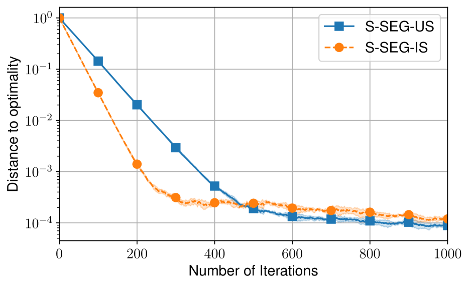
(a) $L_{\max}=2$

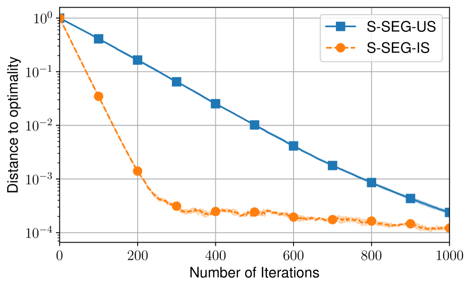
(b) $L_{\max}=5$

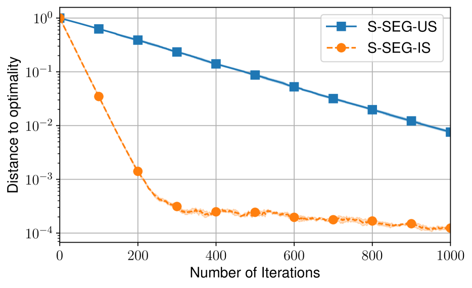
(c) $L_{\max}=10$

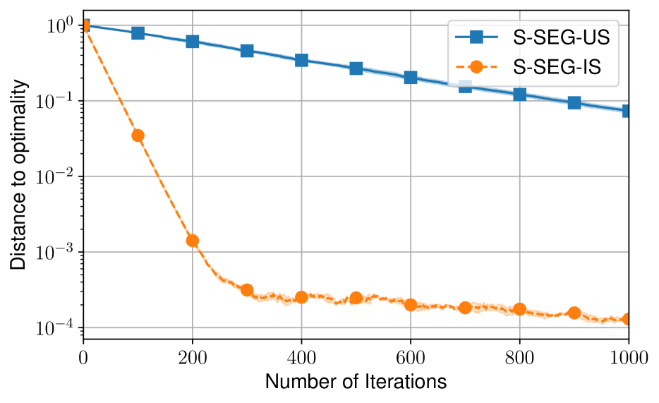
(d) $L_{\max}=20$

Figure 1: Comparison of S-SEG-US vs S-SEG-IS for different values of $L_{\max}$. While the rate of convergence of S-SEG-US becomes slower as $L_{\max}$ increases, the rate of convergence of S-SEG-IS remains the same.

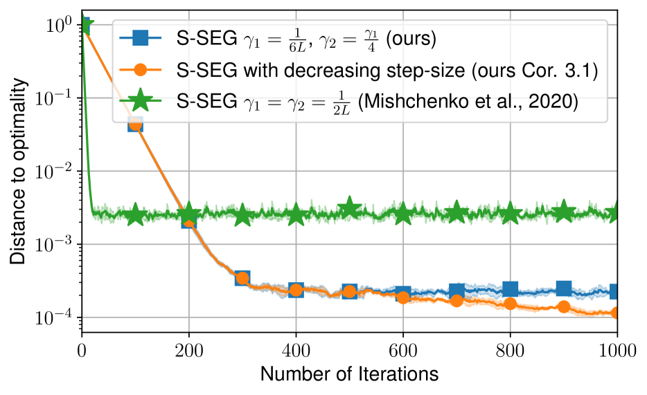
(a)

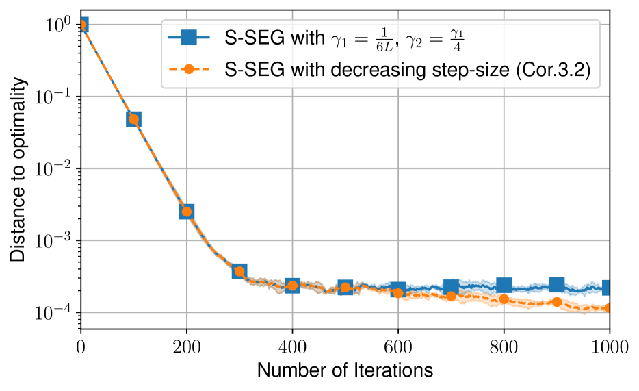
(b)

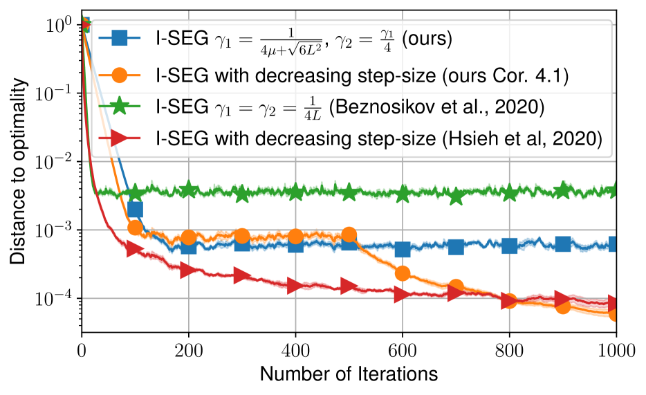
(c)

Figure 2: Experiments on quadratic games illustrating the theoretical results of the paper. (a) Comparison of different stepsize choices for S-SEG. (b) Convergence of S-SEG on quadratic games with negative $\mu_{\xi}$. (c) Comparison of different stepsize choices for I-SEG.

5 NUMERICAL EXPERIMENTS

To illustrate the theoretical results, we conduct experiments on quadratic games of the form:

$$\min_{x_{1}\in\mathbb{R}^{d}}\max_{x_{2}\in\mathbb{R}^{p}}\frac{1}{n}\sum_{i=1}^{n} \frac{1}{2}x_{1}^{\top}\mathbf{A}_{i}x_{1}+x_{1}^{\top}\mathbf{B}_{i}x_{2}-\frac{1}{2}x_{2}^{\top}\mathbf{C}_{i}x_{2}$$

$$\quad+a_{i}^{\top}x_{1}-c_{i}^{\top}x_{2}.$$

By choosing the matrices such that $\mu_{i}\mathbf{I}\preceq{{\bf A}}_{i}\preceq L_{i}\mathbf{I}$ and $\mu_{i}\mathbf{I}\preceq\mathbf{C}_{i}\preceq L_{i}\mathbf{I}$ we can ensure that the game satisfies the assumptions for our theory, i.e., the game is strongly monotone and smooth. In all the experiments, we report the average over 5 different runs. Further details about the experiments can be found in Appendix A.

Experiment 1: S-SEG-US vs S-SEG-IS. To illustrate the advantages of importance sampling compared to uniform sampling, we construct quadratic games such that $L_{1}=L_{\max}$ and $L_{i}=1\quad\forall i>1$. We show in Fig. 1 that while the rate of convergence of S-SEG-US becomes slower as $L_{\max}$ increases, the rate of convergence of S-SEG-IS remains almost the same, because $\overline{L}$ does not change significantly.

Experiment 2: S-SEG with different stepsizes. We compare S-SEG with different stepsize choices in Fig. 2(a). We compare the decreasing stepsize proposed in Corollary 3.1 to the constant stepsize proposed in Mishchenko et al., (2020) where $\gamma_{1}=\gamma_{2}\leq\frac{1}{2L}$, and to the constant stepsize proposed in Theorem 3.1. S-SEG with the proposed decreasing stepsize strategy converges faster to a smaller neighborhood of the solution compared to constant stepsize, see Fig. 2(a).

Experiment 3: Convergence of S-SEG when some $\mu_{\xi}$ are negative. To illustrate the generality of Assumption 3.2, we construct a quadratic game where one of the $\mu_{\xi}$ is negative. We illustrate the generality of Theorem 3.1 in Fig. 2(b) by showing that S-SEG converges to the solution in such games.

Experiment 4: I-SEG with different stepsizes. In Fig. 2(c) we compare I-SEG under different stepsize choices. In particular, we show how the decreasing stepsize strategy proposed in Corollary 4.1 converges to a smaller neighborhood than existing stepsize choices and it has comparable performance to the stepsize rule proposed in Hsieh et al., (2020). However, let us note again that our theoretical rate is better than the one from Hsieh et al., (2020) (see Table 1).

6 CONCLUSION

In this paper, we develop a novel theoretical framework that allows us to analyze several variants of SEG in a unified manner. We provide new convergence analysis for well-known variants of SEG and derive new variants (e.g., S-SEG-IS) that outperform previous SOTA results. However, several important questions remain still open, such as the analysis of SEG for quasi-monotone problems $(\mu=0)$ with unbounded domains without using large batchsizes, the analysis of S-SEG with arbitrary sampling, and the same stepsizes $\gamma_{1,\xi^{k}}=\gamma_{2,\xi^{k}}$, and the improvement of the dependence of $\overline{\mu}$ on negative $\mu_{i}$.

Acknowledgements

This work was partially supported by a grant for research centers in the field of artificial intelligence, provided by the Analytical Center for the Government of the Russian Federation in accordance with the subsidy agreement (agreement identifier 000000D730321P5Q0002) and the agreement with the Moscow Institute of Physics and Technology dated November 1, 2021 No. 70-2021-00138. Part of this work was done while Nicolas Loizou was a postdoctoral research fellow at Mila, Université de Montréal, supported by the IVADO Postdoctoral Funding Program. Gauthier Gidel is supported by an IVADO grant. Part of this work was done while Eduard Gorbunov was an intern at Mila, Université de Montréal under the supervision of Gauthier Gidel and Nicolas Loizou.

 

Supplementary Material:
Stochastic Extragradient: General Analysis and Improved Rates

 

Contents

1. 1 INTRODUCTION
   1. 1.1 Preliminaries
   2. 1.2 Contributions
   3. 1.3 Related Work
   4. 1.4 Paper Organization
2. 2 GENERAL ANALYSIS OF SEG
3. 3 SAME-SAMPLE SEG (S-SEG)
   1. 3.1 Arbitrary Sampling
   2. 3.2 Convergence of S-SEG
4. 4 INDEPENDENT-SAMPLES SEG (I-SEG)
5. 5 NUMERICAL EXPERIMENTS
6. 6 CONCLUSION
7. A ON EXPERIMENTS
   1. A.1 Experimental Details
   2. A.2 Additional Experiment: S-SEG with $b$-Nice Sampling (S-SEG-NICE)
8. B DISCUSSION OF THE RESULTS UNDER QUASI MONOTONICITY
9. C BASIC INEQUALITIES AND AUXILIARY RESULTS
   1. C.1 Basic Inequalities
   2. C.2 Auxiliary Results
10. D GENERAL ANALYSIS OF SEG: MISSING PROOFS
11. E SAME-SAMPLE SEG (S-SEG): MISSING PROOFS AND ADDITIONAL DETAILS
    1. E.1 Details on the Examples of Arbitrary Sampling
    2. E.2 Proof of the Main Result
    3. E.3 S-SEG with Uniform Sampling (S-SEG-US)
    4. E.4 S-SEG with $b$-Nice Sampling (S-SEG-NICE)
    5. E.5 S-SEG with Importance Sampling (S-SEG-IS)
    6. E.6 S-SEG with Independent Sampling Without Replacement (S-SEG-ISWOR)
12. F INDEPENDENT-SAMPLES SEG (I-SEG): MISSING PROOFS AND ADDITIONAL DETAILS
    1. F.1 On the Assumptions in the Analysis of S-SEG and I-SEG

Appendix A ON EXPERIMENTS

A.1 Experimental Details

We describe here in more details the exact settings we use for evaluating the different algorithms. As mentioned in Section 5, we evaluate the different algorithms on the class of quadratic games:

$$\min_{x_{1}\in\mathbb{R}^{d}}\max_{x_{2}\in\mathbb{R}^{p}}\frac{1}{n}\sum_{i}\frac{1}{2}x_{1}^{\top}{\bf A}_{i}x_{1}+x_{1}^{\top}{\bf B}_{i}x_{2}-\frac{1}{2}x_{2}^{\top}{\bf C}_{i}x_{2}+a_{i}^{\top}x_{1}-c_{i}^{\top}x_{2}$$

In all our experiments, we choose $d=p=100$ and $n=100$. To sample the matrices ${\bf A}_{i}$ (resp. ${\bf C}_{i}$) we first generate a random orthogonal matrix ${\bf Q}_{i}$ (resp. ${\bf Q}^{\prime}_{i}$), we then sample a random diagonal matrix ${\bf D}_{i}$ (resp. ${\bf D}^{\prime}_{i}$) where the elements on the diagonal are sampled uniformly in $[\mu_{A},L_{A}]$ (resp. $[\mu_{C},L_{C}]$), such that at least one of the matrices has a minimum eigenvalue equal to $\mu_{A}$ (resp. $\mu_{C}$) and one matrix has a maximum eigenvalue equal to $L_{A}$ (resp. $L_{B}$). Finally we construct the matrices by computing ${\bf A}_{i}={\bf Q}_{i}{\bf D}_{i}{\bf Q}_{i}^{\top}$ (resp. ${\bf C}_{i}={\bf Q}^{\prime}_{i}{\bf D}^{\prime}_{i}{{\bf Q}^{\prime}}_{i}^{\top}$). This ensures that the matrices ${\bf A}_{i}$ and ${\bf C}_{i}$ for all $i\in[n]$, are symmetric and positive definite. We sample the matrices ${\bf B}_{i}$ in a similar fashion with the diagonal matrix ${\bf D}_{i}$ to lie between $[\mu_{B},L_{B}]$. The bias terms $a_{i},c_{i}$ are sampled from a normal distribution. In all our experiments we choose $\mu_{A}=\mu_{C}=0.1$, $L_{A}=L_{C}=1$, $\mu_{B}=0$ and $L_{B}=1$ unless stated otherwise. For further details please refer to the code: https://github.com/hugobb/Stochastic-Extragradient.

A.2 Additional Experiment: S-SEG with $b$-Nice Sampling (S-SEG-NICE)

To illustrate Remark E.1 about the advantages of S-SEG-NICE compared to S-SEG-US with i.i.d. batching, we construct a quadratic game such that $L_{1}=L_{\max}$ and $L_{i}=1,\quad\forall i>1$. We use the constant stepsize specified in Section 3.2. We show in Fig. 3 that the rate of convergence of S-SEG-NICE is faster than S-SEG-US with i.i.d. batching when using the same batch size. However S-SEG-NICE converges to a slightly larger neighborhood of the solution.

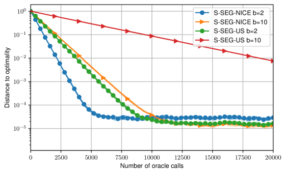
Figure 3: Convergence of S-SEG-NICE for different batchsizes. In this experiment $L_{\max}=10$.

Appendix B DISCUSSION OF THE RESULTS UNDER QUASI MONOTONICITY

Table 2: Summary of the state-of-the-art results for S-SEG and I-SEG for quasi monotone VIPs, i.e., for S-SEG it means that $\overline{\mu}=\frac{1}{n}\sum_{i\in[n]:\mu_{i}\geq 0}\mu_{i}+\frac{4}{n}\sum_{i\in[n]:\mu_{i}<0}\mu_{i}=0$ and for I-SEG – $\mu=0$. Moreover, for I-SEG we assume that $\delta=0$ (see Assumption 4.1). Our results are highlighted in green. Columns: “Norm?” indicates whether the rate is given for the expected squared norm of the operator, “Gap?” indicates whether the rate is given for the expected gap function $\mathbb{E}\left[\text{Gap}_{{\cal C}}(z)\right]=\mathbb{E}\left[\max_{u\in\mathcal{C}}\langle F(u),z-u\rangle\right]$ (here ${\cal C}$ is a compact set containing the solution set), “Unbounded Set?” indicates whether the analysis works for the case of unbounded sets, “$b={\cal O}(1)$?” indicates whether the analysis works with the batchsize independent of the target accuracy of the solution.

Setup	Method	Citation	Norm?	Gap?	Unbounded Set?	$b={\cal O}(1)$?
$F(x)=\frac{1}{n}\sum\limits_{i=1}^{n}F_{i}(x)$ + As. 3.1, 3.2	S-SEG-US	(Mishchenko et al.,, 2020)(1)	✗	✓(2)	✓	✓(3)
		This paper	✓	✗	✓	✗✓(4)
	S-SEG-IS	This paper	✓	✗	✓	✗✓(4)
$F(x)=\mathbb{E}_{\xi}[F_{\xi}(x)]$ + As. 1.1, 1.2, 4.1	I-SEG	(Beznosikov et al.,, 2020)(5)	✗	✓	✗	✓
		This paper	✓	✗	✓	✗

• Mishchenko et al., (2020) consider a regularized version of (VIP) with convex regularization, $F(x)=\mathbb{E}_{\xi}[F_{\xi}(x)]$ and $F_{\xi}(x)$ being monotone and $L_{\xi}$-Lipschitz. If regularization is zero in the obtained problem and $\mathbb{E}_{\xi}[F_{\xi}(x)]=\frac{1}{n}\sum_{i=1}^{n}F_{i}(x)$, the problem from Mishchenko et al., (2020) fits the considered setup with $\mu_{i}=0$ for all $i\in[n]$.

• The rate is derived for $\max_{u\in{\cal C}}\mathbb{E}\left[\langle F(u),\hat{x}^{K}-u\rangle+R(\hat{x}^{K})-R(u)\right]$, where $R(x)$ is the regularization term (in our settings, $R(x)\equiv 0$) and $\hat{x}^{K}$ is the average of the iterates produced by the method. This guarantee is weaker than the one for $\mathbb{E}\left[\text{Gap}_{{\cal C}}(\hat{x}^{K})\right]$.

• Mishchenko et al., (2020) use uniformly bounded variance assumption on a compact set that defines the gap function (Assumption 4.1 with $\delta=0$ on a compact).

• In general, our results in this case require using batchsize dependent on the target accuracy. However, when $F_{i}(x^{*})=0$ for all $i\in[n]$, i.e., when interpolation conditions are satisfied, batchsizes can be chosen arbitrarily, e.g., $b=1$, to achieve the convergence to any predefined accuracy.

• Beznosikov et al., (2020) study a distributed version of I-SEG.

Results under (quasi) monotonicity.

The state-of-the-art results for the convergence of S-SEG and I-SEG for (quasi) monotone VIP are summarized in Table 2. For S-SEG by quasi-monotonicity we mean that Assumption 3.2 holds and $\mathbb{E}_{\xi^{k}}[\gamma_{1,\xi^{k}}\mu_{\xi^{k}}(\mathds{1}_{\{\mu_{\xi^{k}}\geq 0\}}+4\cdot\mathds{1}_{\{\mu_{\xi^{k}}<0\}})]=0$. In the context of finite-sum problems, it means that $\overline{\mu}=\frac{1}{n}\sum_{i\in[n]:\mu_{i}\geq 0}\mu_{i}+\frac{4}{n}\sum_{i\in[n]:\mu_{i}<0}\mu_{i}=0$ both for S-SEG-US and S-SEG-IS. For I-SEG we use the term quasi-monotonicity to describe the problems satisfying Assumption 1.2 with $\mu=0$. The resulting inequality $\langle F(x),x-x^{*}\rangle\geq 0$ is also known as variational stability condition (Hsieh et al.,, 2020; Loizou et al.,, 2021).

The best-known results (Mishchenko et al.,, 2020; Beznosikov et al.,, 2020) provide convergence guarantees in terms of the gap function (Nesterov,, 2007): $\text{Gap}_{{\cal C}}(z)=\max_{u\in{\cal C}}\langle F(u),z-u\rangle$, where ${\cal C}$ is a compact set containing the solution set of (VIP). In particular, Beznosikov et al., (2020) derive a convergence guarantee for $\mathbb{E}[\text{Gap}_{{\cal C}}(\hat{x}^{k})]$, where $\hat{x}^{K}$ is the average of the iterates produced by the method and the problem is assumed to be defined on a compact set. The last requirement is quite restrictive, since many practically important problems are naturally unconstrained. Mishchenko et al., (2020) do not make such an assumption and consider VIPs with regularization, but derive convergence guarantees for $\max_{u\in{\cal C}}\mathbb{E}\left[\langle F(u),\hat{x}^{K}-u\rangle+R(\hat{x}^{K})-R(u)\right]$, where $R(x)$ is the regularization term (in our settings, $R(x)\equiv 0$). That is, when $R(x)\equiv 0$ Mishchenko et al., (2020) obtain upper bounds for $\text{Gap}_{{\cal C}}(\mathbb{E}[\hat{x}^{k}])$ that is a weaker measure of convergence than $\mathbb{E}[\text{Gap}_{{\cal C}}(\hat{x}^{k})]$.

However, Mishchenko et al., (2020); Beznosikov et al., (2020) analyze SEG without using large batchsizes. In contrast, our convergence results for S-SEG and I-SEG are given for the expected squared norm of the operator and hold in the unconstrained case, but, in general, require using target accuracy dependent batchsizes. However, when $F_{\xi}(x^{*})=0$ for all $\xi$, i.e., interpolation conditions are satisfied, our results for S-SEG provide convergence guarantees to any predefined accuracy of the solution even with unit batchsizes ($b=1$).

Last-iterate convergence rates without (quasi) strong monotonicity.

All the results from Table 2 are derived either for the best-iterate or for the averaged-iterate. However, last-iterate convergence results are much more valuable, since the last-iterate is usually used as an output of a method in practical applications. Unfortunately, without additional assumptions a little is known about convergence of SEG in this settings. In fact, even for deterministic EG tight ${\cal O}(\nicefrac{{1}}{{K}})$ last-iterate convergence results were obtained (Golowich et al.,, 2020) under the additional assumption that the Jacobian of $F$ is Lipschitz-continuous, and only recently Gorbunov et al., (2021) derive ${\cal O}(\nicefrac{{1}}{{K}})$ last-iterate convergence rate without using this additional assumption. There are also several linear last-iterate convergence results under the assumption that the operator $F$ is affine and satisfies $\|F(x)\|\geq\mu\|x-x^{*}\|$ ($x^{*}$ is the closest solution to $x$) (Hsieh et al.,, 2020) and under the assumption that $F$ corresponds to the bilinear game (Mishchenko et al.,, 2020).

Appendix C BASIC INEQUALITIES AND AUXILIARY RESULTS

C.1 Basic Inequalities

For all $a,b,a_{1},a_{2},\ldots,a_{n}\in\mathbb{R}^{d}$, $n\geq 1$ the following inequalities hold:

$$\left\|\sum\limits_{i=1}^{n}a_{i}\right\|^{2} \leq n\sum\limits_{i=1}^{n}\|a_{i}\|^{2},$$ (19)

$$\|a+b\|^{2} \geq \frac{1}{2}\|a\|^{2}-\|b\|^{2},$$ (20)

$$2\langle a,b\rangle = \|a\|^{2}+\|b\|^{2}-\|a-b\|^{2}.$$ (21)

C.2 Auxiliary Results

We use the following lemma from Stich, (2019) to derive the final convergence rates from our results on linear convergence to the neighborhood.

Lemma C.1 (Simplified version of Lemma 3 from Stich, (2019)).

Let the non-negative sequence $\{r_{k}\}_{k\geq 0}$ satisfy the relation

$$r_{k+1}\leq(1-a\gamma_{k})r_{k}+c\gamma_{k}^{2}$$

for all $k\geq 0$, parameters $a,c\geq 0$, and any non-negative sequence $\{\gamma_{k}\}_{k\geq 0}$ such that $\gamma_{k}\leq\nicefrac{{1}}{{h}}$ for some $h\geq a$, $h>0$. Then, for any $K\geq 0$ one can choose $\{\gamma_{k}\}_{k\geq 0}$ as follows:

$$\text{if }K\leq\frac{h}{a}, \gamma_{k}=\frac{1}{h},$$

$$\text{if }K>\frac{h}{a}\text{ and }k<k_{0}, \gamma_{k}=\frac{1}{h},$$

$$\text{if }K>\frac{h}{a}\text{ and }k\geq k_{0}, \gamma_{k}=\frac{2}{a(\kappa+k-k_{0})},$$

where $\kappa=\nicefrac{{2h}}{{a}}$ and $k_{0}=\left\lceil\nicefrac{{K}}{{2}}\right\rceil$. For this choice of $\gamma_{k}$ the following inequality holds:

$$r_{K}\leq\frac{32hr_{0}}{a}\exp\left(-\frac{aK}{2h}\right)+\frac{36c}{a^{2}K}.$$

Appendix D GENERAL ANALYSIS OF SEG: MISSING PROOFS

Theorem D.1 (Theorem 2.1).

Consider the method (3). Let Assumption 2.1 hold and $A\leq\nicefrac{{1}}{{2}}$. Then for all $K\geq 0$

$$\mathbb{E}\left[\|x^{K+1}-x^{*}\|^{2}\right]\leq(1+C-\rho)\mathbb{E}\left[\|x^{K}-x^{*}\|^{2}\right]+D_{1}+D_{2},$$ (22)

$$\mathbb{E}\left[\|x^{K}-x^{*}\|^{2}\right]\leq(1+C-\rho)^{K}\|x^{0}-x^{*}\|^{2}+\frac{D_{1}+D_{2}}{\rho-C},$$ (23)

when $\rho>C\geq 0$, and

$$\frac{1}{K+1}\sum\limits_{k=0}^{K}\mathbb{E}[G_{k}]\leq\frac{\|x^{0}-x^{*}\|^{2}}{B(K+1)}+\frac{D_{1}+D_{2}}{B},$$ (24)

when $\rho=C=0$ and $B>0$.

Proof.

Since $x^{k+1}=x^{k}-\gamma_{\xi^{k}}g_{\xi^{k}}(x^{k})$, we have

$$\|x^{k+1}-x^{*}\|^{2} = \|x^{k}-\gamma_{\xi^{k}}g_{\xi^{k}}(x^{k})-x^{*}\|^{2}$$

$$= \|x^{k}-x^{*}\|^{2}-2\gamma_{\xi^{k}}\langle g_{\xi^{k}}(x^{k}),x^{k}-x^{*}\rangle+\gamma_{\xi^{k}}^{2}\|g_{\xi^{k}}(x^{k})\|^{2}.$$

Taking the expectation, conditioned on $\xi^{k}$, using our Assumption 2.1 and the definition of $P_{k}=\mathbb{E}_{\xi^{k}}\left[\gamma_{\xi^{k}}\langle g_{\xi^{k}}(x^{k}),x^{k}-x^{*}\rangle\right]$, we continue our derivation:

$$\mathbb{E}_{\xi^{k}}\left[\|x^{k+1}-x^{*}\|^{2}\right] = \|x^{k}-x^{*}\|^{2}-2P_{k}+\mathbb{E}_{\xi^{k}}[\gamma_{\xi^{k}}^{2}\|g_{\xi^{k}}(x^{k})\|^{2}]$$

$$\overset{\eqref{eq:second_moment_bound_general}}{\leq} \|x^{k}-x^{*}\|^{2}-2P_{k}+2AP_{k}+C\|x^{k}-x^{*}\|^{2}+D_{1}$$

$$\overset{A\leq\nicefrac{{1}}{{2}}}{\leq} (1+C)\|x^{k}-x^{*}\|^{2}-P_{k}+D_{1}$$

$$\overset{\eqref{eq:P_k_general}}{\leq} (1+C-\rho)\|x^{k}-x^{*}\|^{2}-BG_{k}+D_{1}+D_{2}.$$

Next, we take the full expectation from the both sides

$$\mathbb{E}\left[\|x^{k+1}-x^{*}\|^{2}\right]\leq(1+C-\rho)\mathbb{E}\left[\|x^{k}-x^{*}\|^{2}\right]-B\mathbb{E}[G_{k}]+D_{1}+D_{2}.$$ (25)

If $\rho>C\geq 0$, then in the above inequality we can get rid of the non-positive term $(-B\mathbb{E}[G_{k}])$

$$\mathbb{E}\left[\|x^{k+1}-x^{*}\|^{2}\right]\leq(1+C-\rho)\mathbb{E}\left[\|x^{k}-x^{*}\|^{2}\right]+D_{1}+D_{2}$$

and get (22). Unrolling the recurrence, we derive (23):

$$\mathbb{E}\left[\|x^{K}-x^{*}\|^{2}\right] \leq (1+C-\rho)^{K}\|x^{0}-x^{*}\|^{2}+(D_{1}+D_{2})\sum\limits_{k=0}^{K-1}(1+C-\rho)^{k}$$

$$\leq (1+C-\rho)^{K}\|x^{0}-x^{*}\|^{2}+(D_{1}+D_{2})\sum\limits_{k=0}^{\infty}(1+C-\rho)^{k}$$

$$= (1+C-\rho)^{K}\|x^{0}-x^{*}\|^{2}+\frac{D_{1}+D_{2}}{\rho-C}.$$

If $\rho=C=0$ and $B>0$, then (25) is equivalent to

$$B\mathbb{E}[G_{k}]\leq\mathbb{E}\left[\|x^{k}-x^{*}\|^{2}\right]-\mathbb{E}\left[\|x^{k+1}-x^{*}\|^{2}\right]+D_{1}+D_{2}.$$

Summing up these inequalities for $k=0,1,\ldots,K$ and dividing the result by $B(K+1)$, we get (24):

$$\frac{1}{K+1}\sum\limits_{k=0}^{K}\mathbb{E}[G_{k}] \leq \frac{1}{B(K+1)}\sum\limits_{k=0}^{K}\left(\mathbb{E}\left[\|x^{k}-x^{*}\|^{2}\right]-\mathbb{E}\left[\|x^{k+1}-x^{*}\|^{2}\right]\right)+\frac{D_{1}+D_{2}}{B(K+1)}$$

$$= \frac{1}{B(K+1)}\left(\|x^{0}-x^{*}\|^{2}-\mathbb{E}\left[\|x^{K+1}-x^{*}\|^{2}\right]\right)+\frac{D_{1}+D_{2}}{B(K+1)}$$

$$\leq \frac{\|x^{0}-x^{*}\|^{2}}{B(K+1)}+\frac{D_{1}+D_{2}}{B(K+1)}.$$

∎

Appendix E SAME-SAMPLE SEG (S-SEG): MISSING PROOFS AND ADDITIONAL DETAILS

In this section, we provide full proofs and missing details from Section 3 on S-SEG. Recall that our analysis of S-SEG based on the three following assumptions:

• $F_{\xi}(x)$ is $L_{\xi}$-Lipschitz: $\|F_{\xi}(x)-F_{\xi}(y)\|\leq L_{\xi}\|x-y\|$ for all $x,y\in\mathbb{R}^{d}$ (Assumption 3.1),

• $F_{\xi}(x)$ is $(\mu_{\xi},x^{*})$-strongly monotone (with possibly negative $\mu_{\xi}$): $\langle F_{\xi}(x)-F_{\xi}(x^{*}),x-x^{*}\rangle\geq\mu_{\xi}\|x-x^{*}\|^{2}$ for all $x\in\mathbb{R}^{d}$ (Assumption 3.2),

• the following conditions (inequalities (8)-(9)) hold:

  $$\mathbb{E}_{\xi^{k}}[\gamma_{1,\xi^{k}}F_{\xi^{k}}(x^{*})]=0,\quad\mathbb{E}_{\xi^{k}}[\gamma_{1,\xi^{k}}\mu_{\xi^{k}}(\mathds{1}_{\{\mu_{\xi^{k}}\geq 0\}}+4\cdot\mathds{1}_{\{\mu_{\xi^{k}}<0\}})]\geq 0.$$

E.1 Details on the Examples of Arbitrary Sampling

In Section 3, we provide several examples when the assumptions above are satisfied. In all examples, we assume that $F(x)$ has a finite-sum form

$$F(x)=\frac{1}{n}\sum\limits_{i=1}^{n}F_{i}(x)$$ (26)

and $F_{i}$ is $L_{i}$-Lipschitz and $(\mu_{i},x^{*})$-strongly monotone. First, we consider S-SEG with independent sampling with replacement, which covers uniform sampling (Example 3.1) and importance sampling (Example 3.3).

Example E.1 (Independent sampling with replacement).

Let random indices $j_{1},\ldots,j_{b}$ are sampled independently from the the distribution ${\cal D}$ such that for $j\sim{\cal D}$ we have $\mathbb{P}\left[j=i\right]=p_{i}>0$ for $i=1,\ldots,n$, $\sum_{i=1}^{n}p_{i}=1$. Let $\xi=(j_{1},\ldots,j_{b})$ and $F_{\xi}(x)=\frac{1}{b}\sum_{l=1}^{b}F_{j_{l}}(x)$. Moreover, assume that

$$\sum\limits_{j_{1},\ldots,j_{b}:\mu_{(j_{1},\ldots,j_{b})}\geq 0}\mu_{(j_{1},\ldots,j_{b})}+4\sum\limits_{j_{1},\ldots,j_{b}:\mu_{(j_{1},\ldots,j_{b})}<0}\mu_{(j_{1},\ldots,j_{b})}\geq 0,$$

where $\mu_{(j_{1},\ldots,j_{b})}\geq\frac{1}{b}\sum_{i=1}^{b}\mu_{j_{l}}$ is such that the operator $\frac{1}{b}\sum_{l=1}^{b}F_{j_{l}}(x)$ is $(\mu_{(j_{1},\ldots,j_{b})},x^{*})$-strongly monotone. For example, the above inequality is satisfied when all $\mu_{i}\geq 0$. Then, Assumptions 3.1 and 3.2 hold with $L_{\xi}\leq\frac{1}{b}\sum_{l=1}^{b}L_{j_{l}}$, $\mu_{\xi}\geq\frac{1}{b}\sum_{i=1}^{b}\mu_{j_{l}}$, and for the stepsize

$$\gamma_{1,\xi}=\frac{\gamma b}{n^{b}p_{\xi}},\quad\gamma>0,\quad p_{\xi}=\mathbb{P}\left[\xi=(j_{1},\ldots,j_{b})\right]=p_{j_{1}}\ldots p_{j_{b}}$$

we have

$$\mathbb{E}_{\xi^{k}}[\gamma_{1,\xi^{k}}F_{\xi^{k}}(x^{*})] = \frac{\gamma}{n^{b}}\sum\limits_{j_{1},\ldots,j_{b}=1}^{n}\sum\limits_{l=1}^{b}F_{j_{l}}(x^{*})=\frac{\gamma}{n}\sum\limits_{i=1}^{n}F_{i}(x^{*})=\gamma F(x^{*})=0$$

and

$$\mathbb{E}_{\xi^{k}}[\gamma_{1,\xi^{k}}\mu_{\xi^{k}}\mathds{1}_{\{\mu_{\xi^{k}}\geq 0\}}+4\gamma_{1,\xi^{k}}\mu_{\xi^{k}}\mathds{1}_{\{\mu_{\xi^{k}}<0\}}] = \frac{\gamma b}{n^{b}}\sum\limits_{j_{1},\ldots,j_{b}:\mu_{(j_{1},\ldots,j_{b})}\geq 0}\mu_{(j_{1},\ldots,j_{b})}$$

$$\quad+\frac{4\gamma b}{n^{b}}\sum\limits_{j_{1},\ldots,j_{b}:\mu_{(j_{1},\ldots,j_{b})}<0}\mu_{(j_{1},\ldots,j_{b})}$$

$$\geq 0,$$

i.e., conditions from (8)-(9) are satisfied.

Taking $b=1$ and $p_{1}=\ldots=p_{n}=\nicefrac{{1}}{{n}}$ in the previous example we recover single-batch uniform sampling (Example 3.1) as as special case. If $p_{i}=\nicefrac{{L_{i}}}{{\sum_{j=1}^{n}L_{j}}}$, then we get single-batch importance sampling (Example 3.3) as a special case of the previous example.

Finally, we consider two without-replacement sampling strategies. The first one called $b$-nice sampling is described in Section 3 (Example 3.2). Below we prove that conditions (8)-(9) hold for this example. For the reader’s convenience, we also provide a complete description of this sampling.

Example E.2 ($b$-nice sampling).

Let $\xi$ be a random subset of size $b\in[n]$ chosen from the uniform distribution on the family of all subsets of $[n]$ of size $b$. Then, for each $S\subseteq[n],|S|=b$ we have

$$p_{S}=\mathbb{P}\left[\xi=S\right]=\frac{1}{\binom{n}{b}}.$$

Next, let $F_{\xi}(x)=\frac{1}{b}\sum_{i\in\xi}F_{i}(x)$ and $\gamma_{1,\xi}=\gamma$. Moreover, assume that

$$\overline{\mu}_{b-{\sf NICE}}=\frac{1}{\binom{n}{b}}\left(\sum\limits_{S\subseteq[n],|S|=b:\mu_{S}\geq 0}\mu_{S}+4\sum\limits_{S\subseteq[n],|S|=b:\mu_{S}<0}\mu_{S}\right)\geq 0,$$

where $\mu_{S}\geq\frac{1}{b}\sum_{i\in S}\mu_{i}$ is such that the operator $\frac{1}{b}\sum_{i\in S}F_{i}(x)$ is $(\mu_{S},x^{*})$-strongly monotone. For example, the above inequality is satisfied when all $\mu_{i}\geq 0$. Then, Assumptions 3.1 and 3.2 hold with $L_{\xi}\leq\frac{1}{b}\sum_{i\in\xi}L_{i}$, $\mu_{\xi}\geq\frac{1}{b}\sum_{i\in\xi}\mu_{i}$, and we have

$$\mathbb{E}_{\xi^{k}}[\gamma_{1,\xi^{k}}F_{\xi^{k}}(x^{*})] = \frac{\gamma}{b\binom{n}{b}}\sum\limits_{S\subseteq[n],|S|=b}\sum\limits_{i\in S}F_{i}(x^{*})=\frac{\gamma\binom{n-1}{b-1}}{\binom{n}{b}b}\sum\limits_{i=1}^{n}F_{i}(x^{*})=\gamma F(x^{*})=0$$

and

$$\mathbb{E}_{\xi^{k}}[\gamma_{1,\xi^{k}}\mu_{\xi^{k}}\mathds{1}_{\{\mu_{\xi^{k}}\geq 0\}}+4\gamma_{1,\xi^{k}}\mu_{\xi^{k}}\mathds{1}_{\{\mu_{\xi^{k}}<0\}}] = \frac{\gamma}{\binom{n}{b}}\sum\limits_{S\subseteq[n],|S|=b:\mu_{S}\geq 0}\mu_{S}$$

$$\quad+\frac{4\gamma}{\binom{n}{b}}\sum\limits_{S\subseteq[n],|S|=b:\mu_{S}<0}\mu_{S}$$

$$= \gamma\overline{\mu}_{b-{\sf NICE}}\geq 0,$$

i.e., conditions from (8)-(9) are satisfied.

The second without-sampling strategy, which we consider, is independent sampling without replacement.

Example E.3 (Independent sampling without replacement).

Let $\xi$ be a random subset of $[n]$ such that each $i$ is picked with probability $p_{i}$ independently from other elements. It means that the size of $\xi$ is a random variable as well and $\mathbb{E}[|\xi|]=\sum_{i=1}^{n}p_{i}$. Next, we define

$$F_{\xi}(x)=\frac{1}{|\xi|}\sum\limits_{i\in\xi}F_{i}(x)$$

and

$$\gamma_{1,\xi}=\frac{\gamma|\xi|}{p_{\xi}2^{n-1}n},\quad p_{\xi}=\mathbb{P}\left[\xi=S\right]=\prod\limits_{i\in S}p_{i}\cdot\prod\limits_{i\not\in S}(1-p_{i})$$

for any $S\subseteq[n]$. Moreover, assume that

$$\sum\limits_{S\subseteq[n]:\mu_{S}\geq 0}|S|\mu_{S}+4\sum\limits_{S\subseteq[n]:\mu_{S}<0}|S|\mu_{S}\geq 0,$$

where $\mu_{S}\geq\frac{1}{|S|}\sum_{i\in S}\mu_{i}$ is such that the operator $\frac{1}{|S|}\sum_{i\in S}F_{i}(x)$ is $(\mu_{S},x^{*})$-strongly monotone. For example, the above inequality is satisfied when all $\mu_{i}\geq 0$. Then, Assumptions 3.1 and 3.2 hold with $L_{\xi}\leq\frac{1}{|\xi|}\sum_{i\in\xi}L_{i}$, $\mu_{\xi}\geq\frac{1}{|\xi|}\sum_{i\in\xi}\mu_{i}$, and we have

$$\mathbb{E}_{\xi^{k}}[\gamma_{1,\xi^{k}}F_{\xi^{k}}(x^{*})] = \frac{\gamma}{2^{n-1}n}\sum\limits_{S\subseteq[n]}\sum\limits_{i\in S}F_{i}(x^{*})=\frac{\gamma}{n}\sum\limits_{i=1}^{n}F_{i}(x^{*})=\gamma F(x^{*})=0$$

and

$$\mathbb{E}_{\xi^{k}}[\gamma_{1,\xi^{k}}\mu_{\xi^{k}}\mathds{1}_{\{\mu_{\xi^{k}}\geq 0\}}+4\gamma_{1,\xi^{k}}\mu_{\xi^{k}}\mathds{1}_{\{\mu_{\xi^{k}}<0\}}] = \frac{\gamma}{2^{n-1}n}\sum\limits_{S\subseteq[n]:\mu_{S}\geq 0}|S|\mu_{S}$$

$$\quad+\frac{4\gamma}{2^{n-1}n}\sum\limits_{S\subseteq[n]:\mu_{S}<0}|S|\mu_{S}$$

$$\geq 0,$$

i.e., conditions from (8)-(9) are satisfied.

E.2 Proof of the Main Result

The proof is based on two lemmas showing that Assumption 2.1 is satisfied.

Lemma E.1.

Let Assumptions 3.1 and 3.2 hold. If $\gamma_{1,\xi^{k}}$ satisfies (8)-(9) and

$$\gamma_{1,\xi^{k}}\leq\frac{1}{4|\mu_{\xi^{k}}|+\sqrt{2}L_{\xi^{k}}}$$ (27)

then $g^{k}=F_{\xi^{k}}\left(x^{k}-\gamma_{1,\xi^{k}}F_{\xi^{k}}(x^{k})\right)$ satisfies the following inequality

$$\mathbb{E}_{\xi^{k}}\left[\gamma_{1,\xi^{k}}^{2}\|g^{k}\|^{2}\right] \leq 4\widehat{P}_{k}+6\mathbb{E}_{\xi^{k}}\left[\gamma_{1,\xi^{k}}^{2}\|F_{\xi^{k}}(x^{*})\|^{2}\right],$$ (28)

where $\widehat{P}_{k}=\mathbb{E}_{\xi^{k}}\left[\gamma_{1,\xi^{k}}\langle g^{k},x^{k}-x^{*}\rangle\right]$.

Proof.

Using the auxiliary iterate $\widehat{x}^{k+1}=x^{k}-\gamma_{1,\xi^{k}}g^{k}$, we get

$$\|\widehat{x}^{k+1}-x^{*}\|^{2} = \|x^{k}-x^{*}\|^{2}-2\gamma_{1,\xi^{k}}\langle x^{k}-x^{*},g^{k}\rangle+\gamma_{1,\xi^{k}}^{2}\|g^{k}\|^{2}$$

$$= \|x^{k}-x^{*}\|^{2}-2\gamma_{1,\xi^{k}}\left\langle x^{k}-\gamma_{1,\xi^{k}}F_{\xi^{k}}(x^{k})-x^{*},g^{k}\right\rangle$$

$$\quad-2\gamma_{1,\xi^{k}}^{2}\langle F_{\xi^{k}}(x^{k}),g^{k}\rangle+\gamma_{1,\xi^{k}}^{2}\|g^{k}\|^{2}$$

$$= \|x^{k}-x^{*}\|^{2}-2\gamma_{1,\xi^{k}}\left\langle x^{k}-\gamma_{1,\xi^{k}}F_{\xi^{k}}(x^{k})-x^{*},g^{k}-F_{\xi^{k}}(x^{*})\right\rangle$$

$$\quad-2\gamma_{1,\xi^{k}}^{2}\langle F_{\xi^{k}}(x^{k}),g^{k}-F_{\xi^{k}}(x^{*})\rangle-2\gamma_{1,\xi^{k}}\langle x^{k}-x^{*},F_{\xi^{k}}(x^{*})\rangle+\gamma_{1,\xi^{k}}^{2}\|g^{k}\|^{2}.$$

Taking the expectation w.r.t. $\xi^{k}$ from the above identity, using $\mathbb{E}_{\xi^{k}}[\gamma_{1,\xi^{k}}\langle x^{k}-x^{*},F_{\xi^{k}}(x^{*})\rangle]=\langle x^{k}-x^{*},\mathbb{E}_{\xi^{k}}[\gamma_{1,\xi^{k}}F_{\xi^{k}}(x^{*})]\rangle\overset{\eqref{eq:SS_SEG_AS_stepsizes_1}}{=}0$, $g^{k}=F_{\xi^{k}}\left(x^{k}-\gamma_{1,\xi^{k}}F_{\xi^{k}}(x^{k})\right)$ and $(\mu_{\xi},x^{*})$-strong monotonicity of $F_{\xi}(x)$, we derive

$$\mathbb{E}_{\xi^{k}}\left[\|\widehat{x}^{k+1}-x^{*}\|^{2}\right] \leq \|x^{k}-x^{*}\|^{2}-2\mathbb{E}_{\xi^{k}}\left[\gamma_{1,{\xi^{k}}}\left\langle x^{k}-\gamma_{1,{\xi^{k}}}F(x^{k},{\xi^{k}})-x^{*},g^{k}-F(x^{*},{\xi^{k}})\right\rangle\right]$$

$$\quad-2\mathbb{E}_{\xi^{k}}\left[\gamma_{1,{\xi^{k}}}^{2}\langle F(x^{k},{\xi^{k}}),g^{k}-F(x^{*},{\xi^{k}})\rangle\right]+\mathbb{E}_{\xi^{k}}\left[\gamma_{1,{\xi^{k}}}^{2}\|g^{k}\|^{2}\right]$$

$$\overset{\eqref{eq:F_xi_str_monotonicity}}{\leq} \|x^{k}-x^{*}\|^{2}-2\mathbb{E}_{\xi^{k}}\left[\gamma_{1,\xi^{k}}\mu_{\xi^{k}}\|x^{k}-x^{*}-\gamma_{1,{\xi^{k}}}F(x^{k},{\xi^{k}})\|^{2}\right]$$

$$\quad-2\mathbb{E}_{\xi^{k}}\left[\gamma_{1,\xi^{k}}^{2}\langle F_{\xi^{k}}(x^{k}),g^{k}-F_{\xi^{k}}(x^{*})\rangle\right]+\mathbb{E}_{\xi^{k}}\left[\gamma_{1,\xi^{k}}^{2}\|g^{k}\|^{2}\right]$$

$$= \|x^{k}-x^{*}\|^{2}-2\mathbb{E}_{\xi^{k}}\left[\gamma_{1,\xi^{k}}\mu_{\xi^{k}}\mathds{1}_{\{\mu_{\xi^{k}}\geq 0\}}\|x^{k}-x^{*}-\gamma_{1,{\xi^{k}}}F(x^{k},{\xi^{k}})\|^{2}\right]$$

$$\quad-2\mathbb{E}_{\xi^{k}}\left[\gamma_{1,\xi^{k}}\mu_{\xi^{k}}\mathds{1}_{\{\mu_{\xi^{k}}<0\}}\|x^{k}-x^{*}-\gamma_{1,{\xi^{k}}}F(x^{k},{\xi^{k}})\|^{2}\right]$$

$$\quad-2\mathbb{E}_{\xi^{k}}\left[\gamma_{1,\xi^{k}}^{2}\langle F_{\xi^{k}}(x^{k}),g^{k}-F_{\xi^{k}}(x^{*})\rangle\right]+\mathbb{E}_{\xi^{k}}\left[\gamma_{1,\xi^{k}}^{2}\|g^{k}\|^{2}\right]$$

$$\overset{\eqref{eq:a+b_lower}}{\leq} \|x^{k}-x^{*}\|^{2}-\mathbb{E}_{\xi^{k}}[\gamma_{1,\xi^{k}}\mu_{\xi^{k}}\mathds{1}_{\{\mu_{\xi^{k}}\geq 0\}}]\|x^{k}-x^{*}\|^{2}$$

$$\quad+2\mathbb{E}_{\xi^{k}}[\gamma_{1,\xi^{k}}^{3}\mu_{\xi^{k}}\mathds{1}_{\{\mu_{\xi^{k}}\geq 0\}}\|F_{\xi^{k}}(x^{k})\|^{2}]$$

$$\quad-2\mathbb{E}_{\xi^{k}}\left[\gamma_{1,\xi^{k}}\mu_{\xi^{k}}\mathds{1}_{\{\mu_{\xi^{k}}<0\}}\|x^{k}-x^{*}-\gamma_{1,{\xi^{k}}}F(x^{k},{\xi^{k}})\|^{2}\right]$$

$$\quad-2\mathbb{E}_{\xi^{k}}\left[\gamma_{1,\xi^{k}}^{2}\langle F_{\xi^{k}}(x^{k}),g^{k}-F_{\xi^{k}}(x^{*})\rangle\right]+\mathbb{E}_{\xi^{k}}\left[\gamma_{1,\xi^{k}}^{2}\|g^{k}\|^{2}\right]$$

$$\overset{\eqref{eq:a+b}}{\leq} \|x^{k}-x^{*}\|^{2}-\mathbb{E}_{\xi^{k}}[\gamma_{1,\xi^{k}}\mu_{\xi^{k}}\mathds{1}_{\{\mu_{\xi^{k}}\geq 0\}}+4\gamma_{1,\xi^{k}}\mu_{\xi^{k}}\mathds{1}_{\{\mu_{\xi^{k}}<0\}}]\|x^{k}-x^{*}\|^{2}$$

$$\quad+\mathbb{E}_{\xi^{k}}\left[\gamma_{1,{\xi^{k}}}^{2}\|g^{k}\|^{2}\right]$$

$$\quad+2\mathbb{E}_{\xi^{k}}\left[\gamma_{1,{\xi^{k}}}^{3}(\mu_{\xi^{k}}\mathds{1}_{\{\mu_{\xi^{k}}\geq 0\}}-2\mu_{\xi^{k}}\mathds{1}_{\{\mu_{\xi^{k}}<0\}}))\|F_{\xi^{k}}(x^{k})\|^{2}\right]$$

$$\quad-\mathbb{E}_{\xi^{k}}\left[\gamma_{1,{\xi^{k}}}^{2}\|g^{k}-F_{\xi^{k}}(x^{*})\|^{2}\right]$$

$$\quad+\mathbb{E}_{\xi^{k}}\left[\gamma_{1,{\xi^{k}}}^{2}\|F_{\xi^{k}}(x^{k})-g^{k}+F_{\xi^{k}}(x^{*})\|^{2}\right]$$

$$\overset{\eqref{eq:inner_product_representation}}{\leq} \|x^{k}-x^{*}\|^{2}-\mathbb{E}_{\xi^{k}}[\gamma_{1,\xi^{k}}\mu_{\xi^{k}}\mathds{1}_{\{\mu_{\xi^{k}}\geq 0\}}+4\gamma_{1,\xi^{k}}\mu_{\xi^{k}}\mathds{1}_{\{\mu_{\xi^{k}}<0\}}]\|x^{k}-x^{*}\|^{2}$$

$$\quad+\mathbb{E}_{\xi^{k}}\left[\gamma_{1,{\xi^{k}}}^{2}\|g^{k}\|^{2}\right]$$

$$\quad-\mathbb{E}_{\xi^{k}}\left[\gamma_{1,{\xi^{k}}}^{2}(1-2\gamma_{1,\xi^{k}}(\mu_{\xi^{k}}\mathds{1}_{\{\mu_{\xi^{k}}\geq 0\}}-2\mu_{\xi^{k}}\mathds{1}_{\{\mu_{\xi^{k}}<0\}}))\|F_{\xi^{k}}(x^{k})\|^{2}\right]$$

$$\quad-\mathbb{E}_{\xi^{k}}\left[\gamma_{1,{\xi^{k}}}^{2}\|g^{k}-F_{\xi^{k}}(x^{*})\|^{2}\right]$$

$$\quad+\mathbb{E}_{\xi^{k}}\left[\gamma_{1,{\xi^{k}}}^{2}\|F_{\xi^{k}}(x^{k})-g^{k}+F_{\xi^{k}}(x^{*})\|^{2}\right]$$

$$\overset{\eqref{eq:SS_SEG_AS_stepsizes_2}}{\leq} \|x^{k}-x^{*}\|^{2}+\mathbb{E}_{\xi^{k}}\left[\gamma_{1,{\xi^{k}}}^{2}\|g^{k}\|^{2}\right]$$

$$\quad-\mathbb{E}_{\xi^{k}}\left[\gamma_{1,{\xi^{k}}}^{2}(1-4\gamma_{1,\xi^{k}}|\mu_{\xi^{k}}|)\|F_{\xi^{k}}(x^{k})\|^{2}\right]$$

$$\quad-\mathbb{E}_{\xi^{k}}\left[\gamma_{1,{\xi^{k}}}^{2}\|g^{k}-F_{\xi^{k}}(x^{*})\|^{2}\right]$$

$$\quad+\mathbb{E}_{\xi^{k}}\left[\gamma_{1,{\xi^{k}}}^{2}\|F_{\xi^{k}}(x^{k})-g^{k}+F_{\xi^{k}}(x^{*})\|^{2}\right],$$

where in the last inequality we use $\mu_{\xi^{k}}\mathds{1}_{\{\mu_{\xi^{k}}\geq 0\}}-2\mu_{\xi^{k}}\mathds{1}_{\{\mu_{\xi^{k}}<0\}}\leq 2|\mu_{\xi^{k}}|$. To upper bound the last two terms we use simple inequalities (20) and (19), and apply $L_{\xi^{k}}$-Lipschitzness of $F_{\xi^{k}}(x)$:

$$\mathbb{E}\left[\|\widehat{x}^{k+1}-x^{*}\|^{2}\mid x^{k}\right] \overset{\eqref{eq:a+b_lower},\eqref{eq:a+b}}{\leq} \|x^{k}-x^{*}\|^{2}+\mathbb{E}_{\xi^{k}}\left[\gamma_{1,\xi^{k}}^{2}\|g^{k}\|^{2}\right]$$

$$\quad-\mathbb{E}_{\xi^{k}}\left[\gamma_{1,{\xi^{k}}}^{2}(1-4\gamma_{1,\xi^{k}}|\mu_{\xi^{k}}|)\|F_{\xi^{k}}(x^{k})\|^{2}\right]$$

$$\quad-\frac{1}{2}\mathbb{E}_{\xi^{k}}\left[\gamma_{1,\xi^{k}}^{2}\|g^{k}\|^{2}\right]+\mathbb{E}_{\xi^{k}}\left[\gamma_{1,\xi^{k}}^{2}\|F_{\xi^{k}}(x^{*})\|^{2}\right]$$

$$\quad+2\mathbb{E}_{\xi^{k}}\left[\gamma_{1,\xi^{k}}^{2}\|F_{\xi^{k}}(x^{k})-g^{k}\|^{2}\right]+2\mathbb{E}_{\xi^{k}}\left[\gamma_{1,\xi^{k}}^{2}\|F_{\xi^{k}}(x^{*})\|^{2}\right]$$

$$= \|x^{k}-x^{*}\|^{2}+\frac{1}{2}\mathbb{E}_{\xi^{k}}\left[\gamma_{1,\xi^{k}}^{2}\|g^{k}\|^{2}\right]$$

$$\quad-\mathbb{E}_{\xi^{k}}\left[\gamma_{1,{\xi^{k}}}^{2}(1-4\gamma_{1,\xi^{k}}|\mu_{\xi^{k}}|)\|F_{\xi^{k}}(x^{k})\|^{2}\right]$$

$$\quad+3\mathbb{E}_{\xi^{k}}\left[\gamma_{1,\xi^{k}}^{2}\|F_{\xi^{k}}(x^{*})\|^{2}\right]$$

$$\quad+2\mathbb{E}_{\xi^{k}}\left[\gamma_{1,\xi^{k}}^{2}\|F_{\xi^{k}}(x^{k})-F_{\xi^{k}}(x^{k}-\gamma_{1,\xi^{k}}F_{\xi^{k}}(x^{k}))\|^{2}\right]$$

$$\overset{\eqref{eq:F_xi_lip}}{\leq} \|x^{k}-x^{*}\|^{2}+\frac{1}{2}\mathbb{E}_{\xi^{k}}\left[\gamma_{1,\xi^{k}}^{2}\|g^{k}\|^{2}\right]+3\mathbb{E}_{\xi^{k}}\left[\gamma_{1,\xi^{k}}^{2}\|F_{\xi^{k}}(x^{*})\|^{2}\right]$$

$$\quad-\mathbb{E}_{\xi^{k}}\left[\gamma_{1,\xi^{k}}^{2}\left(1-4\gamma_{1,\xi^{k}}|\mu_{\xi^{k}}|-2L_{\xi^{k}}^{2}\gamma_{1,\xi^{k}}^{2}\right)\|F_{\xi^{k}}(x^{k})\|^{2}\right]$$

$$\overset{\eqref{eq:SS_SEG_AS_stepsizes_11}}{\leq} \|x^{k}-x^{*}\|^{2}+\frac{1}{2}\mathbb{E}_{\xi^{k}}\left[\gamma_{1,\xi^{k}}^{2}\|g^{k}\|^{2}\right]+3\mathbb{E}_{\xi^{k}}\left[\gamma_{1,\xi^{k}}^{2}\|F(x^{*},\xi^{k})\|^{2}\right],$$

Finally, we use the above inequality together with (E.2):

$$\|x^{k}-x^{*}\|^{2}-2\widehat{P}_{k}+\mathbb{E}_{\xi^{k}}\left[\gamma_{1,\xi^{k}}^{2}\|g^{k}\|^{2}\right] \leq \|x^{k}-x^{*}\|^{2}+\frac{1}{2}\mathbb{E}_{\xi^{k}}\left[\gamma_{1,\xi^{k}}^{2}\|g^{k}\|^{2}\right]+3\mathbb{E}_{\xi^{k}}\left[\gamma_{1,\xi^{k}}^{2}\|F_{\xi^{k}}(x^{*})\|^{2}\right],$$

where $\widehat{P}_{k}=\mathbb{E}_{\xi^{k}}\left[\gamma_{1,\xi^{k}}\langle g^{k},x^{k}-x^{*}\rangle\right]$. Rearranging the terms, we obtain (28). ∎

Lemma E.2.

Let Assumptions 3.1 and 3.2 hold. If $\gamma_{1,\xi^{k}}$ satisfies (8),(9), and (27), then $g^{k}=F_{\xi^{k}}\left(x^{k}-\gamma_{1,\xi^{k}}F_{\xi^{k}}(x^{k})\right)$ satisfies the following inequality

$$\widehat{P}_{k}\geq\widehat{\rho}\|x^{k}-x^{*}\|^{2}+\frac{1}{2}\widehat{G}_{k}-\frac{3}{2}\mathbb{E}_{\xi^{k}}\left[\gamma_{1,\xi^{k}}^{2}\|F_{\xi}^{k}(x^{*})\|^{2}\right]$$ (30)

where $\widehat{P}_{k}=\mathbb{E}_{\xi^{k}}\left[\gamma_{1,\xi^{k}}\langle g^{k},x^{k}-x^{*}\rangle\right]$ and

$$\widehat{\rho}=\frac{1}{2}\mathbb{E}_{\xi^{k}}[\gamma_{1,\xi^{k}}\mu_{\xi^{k}}(\mathds{1}_{\{\mu_{\xi^{k}}\geq 0\}}+4\cdot\mathds{1}_{\{\mu_{\xi^{k}}<0\}})],$$

$$\widehat{G}_{k}=\mathbb{E}_{\xi^{k}}\left[\gamma_{1,\xi^{k}}^{2}\left(1-4|\mu_{\xi^{k}}|\gamma_{1,\xi^{k}}-2L_{\xi^{k}}^{2}\gamma_{1,\xi^{k}}^{2}\right)\|F_{\xi^{k}}(x^{k})\|^{2}\right].$$

Proof.

We start with rewriting $\widehat{P}_{k}$:

$$-\widehat{P}_{k} = -\mathbb{E}_{\xi^{k}}\left[\gamma_{1,\xi^{k}}\langle g^{k},x^{k}-x^{*}\rangle\right]\overset{\eqref{eq:SS_SEG_AS_stepsizes_1}}{=}-\mathbb{E}_{\xi^{k}}\left[\gamma_{1,\xi^{k}}\langle g^{k}-F_{\xi^{k}}(x^{*}),x^{k}-x^{*}\rangle\right]$$ (31)

$$= -\mathbb{E}_{\xi^{k}}\left[\gamma_{1,\xi^{k}}\langle g^{k}-F_{\xi^{k}}(x^{*}),x^{k}-\gamma_{1,\xi^{k}}F_{\xi^{k}}(x^{k})-x^{*}\rangle\right]$$

$$\quad-\mathbb{E}_{\xi^{k}}\left[\gamma_{1,\xi^{k}}^{2}\langle g^{k}-F_{\xi^{k}}(x^{*}),F_{\xi^{k}}(x^{k})\rangle\right]$$

$$\overset{\eqref{eq:inner_product_representation}}{=} \underbrace{-\mathbb{E}_{\xi^{k}}\left[\gamma_{1,\xi^{k}}\left\langle F_{\xi^{k}}(x^{k}-\gamma_{1,\xi^{k}}F_{\xi^{k}}(x^{k}))-F_{\xi^{k}}(x^{*}),x^{k}-\gamma_{1,\xi^{k}}F_{\xi^{k}}(x^{k})-x^{*}\right\rangle\right]}_{T_{1}}$$

$$\quad\underbrace{-\frac{1}{2}\mathbb{E}_{\xi^{k}}\left[\gamma_{1,\xi^{k}}^{2}\|g^{k}-F_{\xi^{k}}(x^{*})\|^{2}\right]+\frac{1}{2}\mathbb{E}_{\xi^{k}}\left[\gamma_{1,\xi^{k}}^{2}\|g^{k}-F_{\xi^{k}}(x^{k})-F_{\xi^{k}}(x^{*})\|^{2}\right]}_{T_{2}}$$

$$\quad-\frac{1}{2}\mathbb{E}_{\xi^{k}}\left[\gamma_{1,\xi^{k}}^{2}\|F_{\xi^{k}}(x^{k})\|^{2}\right].$$

Next, we upper bound terms $T_{1}$ and $T_{2}$. From $(\mu_{\xi^{k}},x^{*})$-strong monotonicity of $F_{\xi^{k}}$ we have

$$T_{1} \overset{\eqref{eq:F_xi_str_monotonicity}}{\leq} -\mathbb{E}_{\xi^{k}}\left[\mu_{\xi^{k}}\gamma_{1,\xi^{k}}\left\|x^{k}-x^{*}-\gamma_{1,\xi^{k}}F_{\xi^{k}}(x^{K})\right\|^{2}\right]$$

$$= -\mathbb{E}_{\xi^{k}}\left[\mathds{1}_{\{\mu_{\xi^{k}}\geq 0\}}\mu_{\xi^{k}}\gamma_{1,\xi^{k}}\left\|x^{k}-x^{*}-\gamma_{1,\xi^{k}}F_{\xi^{k}}(x^{K})\right\|^{2}\right]$$

$$\quad-\mathbb{E}_{\xi^{k}}\left[\mathds{1}_{\{\mu_{\xi^{k}}<0\}}\mu_{\xi^{k}}\gamma_{1,\xi^{k}}\left\|x^{k}-x^{*}-\gamma_{1,\xi^{k}}F_{\xi^{k}}(x^{K})\right\|^{2}\right]$$

$$\overset{\eqref{eq:a+b_lower},\eqref{eq:a+b}}{\leq} -\frac{1}{2}\mathbb{E}_{\xi^{k}}\left[\mathds{1}_{\{\mu_{\xi^{k}}\geq 0\}}\mu_{\xi^{k}}\gamma_{1,\xi^{k}}\right]\|x^{k}-x^{*}\|^{2}+\mathbb{E}_{\xi^{k}}\left[\mathds{1}_{\{\mu_{\xi^{k}}\geq 0\}}\mu_{\xi^{k}}\gamma_{1,\xi^{k}}^{3}\|F_{\xi^{k}}(x^{k})\|^{2}\right]$$

$$\quad-2\mathbb{E}_{\xi^{k}}\left[\mathds{1}_{\{\mu_{\xi^{k}}<0\}}\mu_{\xi^{k}}\gamma_{1,\xi^{k}}\right]\|x^{k}-x^{*}\|^{2}-2\mathbb{E}_{\xi^{k}}\left[\mathds{1}_{\{\mu_{\xi^{k}}<0\}}\mu_{\xi^{k}}\gamma_{1,\xi^{k}}^{3}\|F_{\xi^{k}}(x^{k})\|^{2}\right]$$

$$\leq -\frac{1}{2}\mathbb{E}_{\xi^{k}}\left[\left(\mathds{1}_{\{\mu_{\xi^{k}}\geq 0\}}+4\cdot\mathds{1}_{\{\mu_{\xi^{k}}<0\}}\right)\mu_{\xi^{k}}\gamma_{1,\xi^{k}}\right]\|x^{k}-x^{*}\|^{2}+2\mathbb{E}_{\xi^{k}}\left[|\mu_{\xi^{k}}|\gamma_{1,\xi^{k}}^{3}\|F_{\xi^{k}}(x^{k})\|^{2}\right].$$

Using simple inequalities (20) and (19) and applying $L_{\xi^{k}}$-Lipschitzness of $F_{\xi^{k}}(x)$, we upper bound $T_{2}$:

$$T_{2} \overset{\eqref{eq:a+b_lower},\eqref{eq:a+b}}{\leq} -\frac{1}{4}\mathbb{E}_{\xi^{k}}\left[\gamma_{1,\xi^{k}}^{2}\|g^{k}\|^{2}\right]+\frac{1}{2}\mathbb{E}\left[\gamma_{1,\xi^{k}}^{2}\|F_{\xi^{k}}(x^{*})\|^{2}\right]$$

$$\quad+\mathbb{E}_{\xi^{k}}\left[\gamma_{1,\xi^{k}}^{2}\|g^{k}-F_{\xi^{k}}(x^{k})\|^{2}\right]+\mathbb{E}_{\xi^{k}}\left[\gamma_{1,\xi^{k}}^{2}\|F_{\xi^{k}}(x^{*})\|^{2}\right]$$

$$\leq \mathbb{E}_{\xi^{k}}\left[\gamma_{1,\xi^{k}}^{2}\|g^{k}-F_{\xi^{k}}(x^{k})\|^{2}\right]+\frac{3}{2}\mathbb{E}_{\xi^{k}}\left[\gamma_{1,\xi^{k}}^{2}\|F_{\xi^{k}}(x^{*})\|^{2}\right]$$

$$= \mathbb{E}_{\xi^{k}}\left[\gamma_{1,\xi^{k}}^{2}\|F_{\xi^{k}}(x^{k}-\gamma_{1,\xi^{k}}F_{\xi^{k}}(x^{k}))-F_{\xi^{k}}(x^{k})\|^{2}\right]+\frac{3}{2}\mathbb{E}_{\xi^{k}}\left[\gamma_{1,\xi^{k}}^{2}\|F_{\xi^{k}}(x^{*})\|^{2}\right]$$

$$\overset{\eqref{eq:F_xi_lip}}{\leq} \mathbb{E}_{\xi^{k}}\left[L_{\xi^{k}}^{2}\gamma_{1,\xi^{k}}^{4}\|F_{\xi^{k}}(x^{k})\|^{2}\right]+\frac{3}{2}\mathbb{E}_{\xi^{k}}\left[\gamma_{1,\xi^{k}}^{2}\|F_{\xi^{k}}(x^{*})\|^{2}\right].$$

Putting all together in (31), we derive

$$-\widehat{P}_{k} \leq -\frac{1}{2}\mathbb{E}_{\xi^{k}}\left[\left(\mathds{1}_{\{\mu_{\xi^{k}}\geq 0\}}+4\cdot\mathds{1}_{\{\mu_{\xi^{k}}<0\}}\right)\mu_{\xi^{k}}\gamma_{1,\xi^{k}}\right]\|x^{k}-x^{*}\|^{2}+\frac{3}{2}\mathbb{E}_{\xi^{k}}\left[\gamma_{1,\xi^{k}}^{2}\|F_{\xi^{k}}(x^{*})\|^{2}\right]$$

$$\quad-\frac{1}{2}\mathbb{E}_{\xi^{k}}\left[\gamma_{1,\xi^{k}}^{2}\left(1-4|\mu_{\xi^{k}}|\gamma_{1,\xi^{k}}-2L_{\xi^{k}}^{2}\gamma_{1,\xi^{k}}^{2}\right)\|F_{\xi^{k}}(x^{k})\|^{2}\right],$$

where the last term is non-negative due to (27). This finishes the proof. ∎

Combining two previous lemmas with Theorem 2.1, we derive the following result.

Theorem E.1 (Theorem 3.1).

Let Assumptions 3.1 and 3.2 hold. If $\gamma_{2,\xi^{k}}=\alpha\gamma_{1,\xi_{k}}$, $\alpha>0$, and $\gamma_{1,\xi^{k}}$ satisfies (8), (9), and (27), then $g^{k}=F_{\xi^{k}}\left(x^{k}-\gamma_{1,\xi^{k}}F_{\xi^{k}}(x^{k})\right)$ from (S-SEG) satisfies Assumption 2.1 with the following parameters:

$$A=2\alpha,\quad C=0,\quad D_{1}=6\alpha^{2}\sigma_{{\sf AS}}^{2}=6\alpha^{2}\mathbb{E}_{\xi}\left[\gamma_{1,\xi}^{2}\|F_{\xi}(x^{*})\|^{2}\right],$$

$$\rho=\frac{\alpha}{2}\mathbb{E}_{\xi^{k}}[\gamma_{1,\xi^{k}}\mu_{\xi^{k}}(\mathds{1}_{\{\mu_{\xi^{k}}\geq 0\}}+4\cdot\mathds{1}_{\{\mu_{\xi^{k}}<0\}})],$$

$$G_{k}=\alpha\mathbb{E}_{\xi^{k}}\left[\gamma_{1,\xi^{k}}^{2}\left(1-4|\mu_{\xi^{k}}|\gamma_{1,\xi^{k}}-2L_{\xi^{k}}^{2}\gamma_{1,\xi^{k}}^{2}\right)\|F_{\xi^{k}}(x^{k})\|^{2}\right],\quad B=\frac{1}{2},\quad D_{2}=\frac{3\alpha}{2}\sigma_{{\sf AS}}^{2}.$$

If additionally $\alpha\leq\nicefrac{{1}}{{4}}$, then for all $K\geq 0$ we have for the case $\rho>0$

$$\mathbb{E}\left[\|x^{K+1}-x^{*}\|^{2}\right]\leq\left(1-\rho\right)\mathbb{E}\left[\|x^{K}-x^{*}\|^{2}\right]+\frac{3\alpha}{2}\left(4\alpha+1\right)\sigma_{{\sf AS}}^{2},$$

$$\mathbb{E}\left[\|x^{K}-x^{*}\|^{2}\right]\leq\left(1-\rho\right)^{K}\|x^{0}-x^{*}\|^{2}+\frac{3\alpha\left(4\alpha+1\right)\sigma_{{\sf AS}}^{2}}{2\rho},$$

and for the case $\rho=0$

$$\frac{1}{K+1}\sum\limits_{k=0}^{K}\mathbb{E}\left[\gamma_{1,\xi^{k}}^{2}\left(1-4|\mu_{\xi^{k}}|\gamma_{1,\xi^{k}}-2L_{\xi^{k}}^{2}\gamma_{1,\xi^{k}}^{2}\right)\|F_{\xi^{k}}(x^{k})\|^{2}\right]\leq\frac{2\|x^{0}-x^{*}\|^{2}}{\alpha(K+1)}+3(4\alpha+1)\sigma_{{\sf AS}}^{2}.$$

Proof.

S-SEG fits the unified update rule (3) with $\gamma_{\xi^{k}}=\gamma_{2,\xi^{k}}$ and $g^{k}=F_{\xi^{k}}\left(x^{k}-\gamma_{1,\xi^{k}}F_{\xi^{k}}(x^{k})\right)$. Moreover, Lemmas E.1 and E.2 imply

$$\mathbb{E}_{\xi^{k}}\left[\gamma_{1,\xi^{k}}^{2}\|g^{k}\|^{2}\right] \leq 4\widehat{P}_{k}+6\mathbb{E}_{\xi^{k}}\left[\gamma_{1,\xi^{k}}^{2}\|F_{\xi^{k}}(x^{*})\|^{2}\right],$$ (32)

$$\widehat{P}_{k} \geq \widehat{\rho}\|x^{k}-x^{*}\|^{2}+\frac{1}{2}\widehat{G}_{k}-\frac{3}{2}\mathbb{E}_{\xi^{k}}\left[\gamma_{1,\xi^{k}}^{2}\|F_{\xi}^{k}(x^{*})\|^{2}\right],$$ (33)

where $\widehat{P}_{k}=\mathbb{E}_{\xi^{k}}\left[\gamma_{1,\xi^{k}}\langle g^{k},x^{k}-x^{*}\rangle\right]$ and

$$\widehat{\rho}=\frac{1}{2}\mathbb{E}_{\xi^{k}}[\gamma_{1,\xi^{k}}\mu_{\xi^{k}}(\mathds{1}_{\{\mu_{\xi^{k}}\geq 0\}}+4\cdot\mathds{1}_{\{\mu_{\xi^{k}}<0\}})],$$

$$\widehat{G}_{k}=\mathbb{E}_{\xi^{k}}\left[\gamma_{1,\xi^{k}}^{2}\left(1-4|\mu_{\xi^{k}}|\gamma_{1,\xi^{k}}-2L_{\xi^{k}}^{2}\gamma_{1,\xi^{k}}^{2}\right)\|F_{\xi^{k}}(x^{k})\|^{2}\right].$$

Since $\gamma_{\xi^{k}}=\gamma_{2,\xi^{k}}=\alpha\gamma_{1,\xi^{k}}$, we multiply (32) by $\alpha^{2}$ and (33) by $\alpha$ and get that Assumption 2.1 holds with the parameters given in the statement of the theorem. Applying Theorem 2.1 we get the result. ∎

The next corollary establishes the convergence rate with diminishing stepsizes allowing to reduce the size of the neighborhood, when $\rho>0$.

Corollary E.1 ($\rho>0$; Corollary 3.1).

Let Assumptions 3.1 and 3.2 hold, $\gamma_{2,\xi^{k}}=\alpha\gamma_{1,\xi_{k}}$, $\alpha=\nicefrac{{1}}{{4}}$, $\gamma_{1,\xi^{k}}=\beta_{k}\cdot\gamma_{\xi^{k}}$, and $\gamma_{\xi^{k}}$ satisfies (8), (9), and (27). Assume that

$$\widetilde{\rho}=\frac{1}{8}\mathbb{E}_{\xi^{k}}[\gamma_{\xi^{k}}\mu_{\xi^{k}}(\mathds{1}_{\{\mu_{\xi^{k}}\geq 0\}}+4\cdot\mathds{1}_{\{\mu_{\xi^{k}}<0\}})]>0.$$

Then, for all $K\geq 0$ and $\{\beta_{k}\}_{k\geq 0}$ such that

$$\text{if }K\leq\frac{1}{\widetilde{\rho}}, \beta_{k}=1,$$

$$\text{if }K>\frac{1}{\widetilde{\rho}}\text{ and }k<k_{0}, \beta_{k}=1,$$

$$\text{if }K>\frac{1}{\widetilde{\rho}}\text{ and }k\geq k_{0}, \beta_{k}=\frac{2}{2+\widetilde{\rho}(k-k_{0})},$$

for $k_{0}=\left\lceil\nicefrac{{K}}{{2}}\right\rceil$ we have

$$\mathbb{E}\left[\|x^{K}-x^{*}\|^{2}\right]\leq\frac{32\|x^{0}-x^{*}\|^{2}}{\widetilde{\rho}}\exp\left(-\frac{\widetilde{\rho}K}{2}\right)+\frac{27\sigma_{{\sf AS}}^{2}}{\widetilde{\rho}^{2}K},$$

where $\sigma_{{\sf AS}}^{2}=\mathbb{E}_{\xi}\left[\gamma_{\xi}^{2}\|F_{\xi}(x^{*})\|^{2}\right]$

Proof.

In Theorem E.1, we establish the following recurrence:

$$\mathbb{E}\left[\|x^{k+1}-x^{*}\|^{2}\right] \leq \left(1-\beta_{k}\widetilde{\rho}\right)\mathbb{E}\left[\|x^{k}-x^{*}\|^{2}\right]+\frac{3\alpha}{2}\left(4\alpha+1\right)\beta_{k}^{2}\sigma_{{\sf AS}}^{2}$$

$$\overset{\alpha=\nicefrac{{1}}{{4}}}{=} \left(1-\beta_{k}\widetilde{\rho}\right)\mathbb{E}\left[\|x^{k}-x^{*}\|^{2}\right]+\beta_{k}^{2}\frac{3\sigma_{{\sf AS}}^{2}}{4},$$

where we redefined $\rho$ and $\sigma_{{\sf AS}}^{2}$ to better handle decreasing stepsizes. Applying Lemma C.1 for $r_{k}=\mathbb{E}\left[\|x^{k}-x^{*}\|^{2}\right]$, $\gamma_{k}=\beta_{k}$, $a=\widetilde{\rho}$, $c=\nicefrac{{3\sigma_{{\sf AS}}^{2}}}{{4}}$, $h=1$, we get the result. ∎

When $\rho=0$, we use large batchiszes to reduce the size of the neighborhood.

Corollary E.2 ($\rho=0$).

Let Assumptions 3.1 and 3.2 hold, $\gamma_{2,\xi^{k}}=\alpha\gamma_{1,\xi_{k}}$, $\alpha=\nicefrac{{1}}{{4}}$, and $\gamma_{1,\xi^{k}}$ satisfies (8)-(9), and

$$0<\gamma_{1,\xi^{k}}\leq\frac{1}{8|\mu_{\xi^{k}}|+2\sqrt{2}L_{\xi^{k}}}.$$

Assume that

$$\rho=\frac{1}{8}\mathbb{E}_{\xi^{k}}[\gamma_{1,\xi^{k}}\mu_{\xi^{k}}(\mathds{1}_{\{\mu_{\xi^{k}}\geq 0\}}+4\cdot\mathds{1}_{\{\mu_{\xi^{k}}<0\}})]=0,$$

$$\mathbb{E}_{\xi^{k}}\left[\gamma_{1,\xi^{k}}F_{\xi^{k}}(x^{k})\right]=\gamma F(x^{k})$$

for some $\gamma>0$ and $F_{\xi^{k}}(x^{k})$ is computed via ${\cal O}(b)$ stochastic oracle calls and

$$\mathbb{E}_{\xi^{k}\sim{\cal D}}\left[\gamma_{1,\xi^{k}}^{2}\|F_{\xi^{k}}(x^{*})\|^{2}\right]\leq\frac{1}{b}\mathbb{E}_{\xi^{k}\sim\widehat{{\cal D}}}\left[\gamma_{1,\xi^{k}}^{2}\|F_{\xi^{k}}(x^{*})\|^{2}\right]=\frac{\sigma_{{\sf AS}}^{2}}{b},$$

where $\widehat{{\cal D}}$ satisfies Assumptions 3.1 and 3.2. Then, for all $K\geq 0$ we have

$$\frac{1}{K+1}\sum\limits_{k=0}^{K}\mathbb{E}\left[\|F(x^{k})\|^{2}\right]\leq\frac{16\|x^{0}-x^{*}\|^{2}}{\gamma^{2}(K+1)}+\frac{12\sigma_{{\sf AS}}^{2}}{\gamma^{2}b},$$

and each iteration requires ${\cal O}(b)$ stochastic oracle calls.

Proof.

Theorem E.1 implies that

$$\frac{1}{K+1}\sum\limits_{k=0}^{K}\mathbb{E}\left[\gamma_{1,\xi^{k}}^{2}\left(1-4|\mu_{\xi^{k}}|\gamma_{1,\xi^{k}}-2L_{\xi^{k}}^{2}\gamma_{1,\xi^{k}}^{2}\right)\|F_{\xi^{k}}(x^{k})\|^{2}\right]$$

$$\leq\frac{2\|x^{0}-x^{*}\|^{2}}{\alpha(K+1)}+3(4\alpha+1)\mathbb{E}_{\xi^{k}\sim{\cal D}}\left[\gamma_{1,\xi^{k}}^{2}\|F_{\xi^{k}}(x^{*})\|^{2}\right]$$

$$\overset{\alpha=\nicefrac{{1}}{{4}}}{\leq}\frac{8\|x^{0}-x^{*}\|^{2}}{K+1}+\frac{6\sigma_{{\sf AS}}^{2}}{b}.$$

Since

$$0<\gamma_{1,\xi^{k}}\leq\frac{1}{8|\mu_{\xi^{k}}|+2\sqrt{2}L_{\xi^{k}}},$$

we have

$$\frac{1}{2(K+1)}\sum\limits_{k=0}^{K}\mathbb{E}\left[\gamma_{1,\xi^{k}}^{2}\|F_{\xi^{k}}(x^{k})\|^{2}\right] \leq \frac{8\|x^{0}-x^{*}\|^{2}}{K+1}+\frac{6\sigma_{{\sf AS}}^{2}}{b}.$$

Finally, we use Jensen’s inequality and $\mathbb{E}_{\xi^{k}}\left[\gamma_{1,\xi^{k}}F_{\xi^{k}}(x^{k})\right]=\gamma F(x^{k})$:

$$\frac{\gamma^{2}}{2(K+1)}\sum\limits_{k=0}^{K}\mathbb{E}\left[\|F(x^{k})\|^{2}\right] = \frac{1}{2(K+1)}\sum\limits_{k=0}^{K}\mathbb{E}\left[\left\|\mathbb{E}_{\xi^{k}}\left[\gamma_{1,\xi^{k}}F_{\xi^{k}}(x^{k})\right]\right\|^{2}\right]$$

$$\leq \frac{1}{2(K+1)}\sum\limits_{k=0}^{K}\mathbb{E}\left[\mathbb{E}_{\xi^{k}}\left[\left\|\gamma_{1,\xi^{k}}F_{\xi^{k}}(x^{k})\right\|^{2}\right]\right]$$

$$= \frac{1}{2(K+1)}\sum\limits_{k=0}^{K}\mathbb{E}\left[\gamma_{1,\xi^{k}}^{2}\|F_{\xi^{k}}(x^{k})\|^{2}\right]$$

$$\leq \frac{8\|x^{0}-x^{*}\|^{2}}{K+1}+\frac{6\sigma_{{\sf AS}}^{2}}{b}.$$

Multiplying the inequality by $\nicefrac{{2}}{{\gamma^{2}}}$, we get the result. ∎

E.3 S-SEG with Uniform Sampling (S-SEG-US)

Theorem E.2.

Consider the setup from Example 3.1. If $\gamma_{2,\xi^{k}}=\alpha\gamma_{1,\xi_{k}}$, $\alpha>0$, and $\gamma_{1,\xi^{k}}=\gamma\leq\nicefrac{{1}}{{6L_{\max}}}$, where $L_{\max}=\max_{i\in[n]}L_{i}$, then $g^{k}=F_{\xi^{k}}\left(x^{k}-\gamma_{1,\xi^{k}}F_{\xi^{k}}(x^{k})\right)$ from (S-SEG) satisfies Assumption 2.1 with the following parameters:

$$A=2\alpha,\quad C=0,\quad D_{1}=6\alpha^{2}\gamma^{2}\sigma_{{\sf US*}}^{2}=\frac{6\alpha^{2}\gamma^{2}}{n}\sum\limits_{i=1}^{n}\|F_{i}(x^{*})\|^{2},\quad\rho=\frac{\alpha\gamma\overline{\mu}}{2},$$

$$G_{k}=\frac{\alpha\gamma^{2}}{n}\sum\limits_{i=1}^{n}\left(1-4|\mu_{i}|\gamma-2L_{i}^{2}\gamma^{2}\right)\|F_{i}(x^{k})\|^{2},\quad B=\frac{1}{2},\quad D_{2}=\frac{3\alpha\gamma^{2}}{2}\sigma_{{\sf US*}}^{2}.$$

If additionally $\alpha\leq\nicefrac{{1}}{{4}}$, then for all $K\geq 0$ we have for the case $\overline{\mu}>0$

$$\mathbb{E}\left[\|x^{K+1}-x^{*}\|^{2}\right]\leq\left(1-\frac{\alpha\gamma\overline{\mu}}{2}\right)\mathbb{E}\left[\|x^{K}-x^{*}\|^{2}\right]+\frac{3\alpha}{2}\left(4\alpha+1\right)\gamma^{2}\sigma_{{\sf US*}}^{2},$$

$$\mathbb{E}\left[\|x^{K}-x^{*}\|^{2}\right]\leq\left(1-\frac{\alpha\gamma\overline{\mu}}{2}\right)^{K}\|x^{0}-x^{*}\|^{2}+\frac{3\left(4\alpha+1\right)\gamma\sigma_{{\sf US*}}^{2}}{\overline{\mu}},$$

and for the case $\overline{\mu}=0$

$$\frac{1}{K+1}\sum\limits_{k=0}^{K}\mathbb{E}\left[\frac{1}{n}\sum\limits_{i=1}^{n}\left(1-4|\mu_{i}|\gamma-2L_{i}^{2}\gamma^{2}\right)\|F_{i}(x^{k})\|^{2}\right]\leq\frac{2\|x^{0}-x^{*}\|^{2}}{\alpha\gamma^{2}(K+1)}+3(4\alpha+1)\sigma_{{\sf US*}}^{2}.$$

Proof.

Since $\gamma\leq\nicefrac{{1}}{{6L_{\max}}}$ and $|\mu_{i}|\leq L_{i}$, condition (27) is satisfied. In Example E.1, we show that conditions (8) and (9) hold as well. Therefore, Theorem E.1 implies the desired result with

$$\sigma_{{\sf AS}}^{2} = \mathbb{E}_{\xi}\left[\gamma_{1,\xi}^{2}\|F_{\xi}(x^{*})\|^{2}\right]=\frac{\gamma^{2}}{n}\sum_{i=1}^{n}\|F_{i}(x^{*})\|^{2}=\gamma^{2}\sigma_{{\sf US}*}^{2},$$

$$\rho = \frac{\alpha}{2}\mathbb{E}_{\xi^{k}}[\gamma_{1,\xi^{k}}\mu_{\xi^{k}}(\mathds{1}_{\{\mu_{\xi^{k}}\geq 0\}}+4\cdot\mathds{1}_{\{\mu_{\xi^{k}}<0\}})]=\frac{\alpha\gamma}{2n}\left(\sum\limits_{i:\mu_{i}\geq 0}\mu_{i}+4\sum\limits_{i:\mu_{i}<0}\mu_{i}\right)=\frac{\alpha\gamma\overline{\mu}}{2},$$

$$G_{k} = \alpha\mathbb{E}_{\xi^{k}}\left[\gamma_{1,\xi^{k}}^{2}\left(1-4|\mu_{\xi^{k}}|\gamma_{1,\xi^{k}}-2L_{\xi^{k}}^{2}\gamma_{1,\xi^{k}}^{2}\right)\|F_{\xi^{k}}(x^{k})\|^{2}\right]$$

$$= \frac{\alpha\gamma^{2}}{n}\sum\limits_{i=1}^{n}\left(1-4|\mu_{i}|\gamma-2L_{i}^{2}\gamma^{2}\right)\|F_{i}(x^{k})\|^{2}.$$

∎

Corollary E.3 ($\overline{\mu}>0$).

Consider the setup from Example 3.1. Let $\overline{\mu}>0$, $\gamma_{2,\xi^{k}}=\alpha\gamma_{1,\xi_{k}}$, $\alpha=\nicefrac{{1}}{{4}}$, and $\gamma_{1,\xi^{k}}=\beta_{k}\gamma=\nicefrac{{\beta_{k}}}{{6L_{\max}}}$, where $L_{\max}=\max_{i\in[n]}L_{i}$ and $0<\beta_{k}\leq 1$. Then, for all $K\geq 0$ and $\{\beta_{k}\}_{k\geq 0}$ such that

$$\text{if }K\leq\frac{48L_{\max}}{\overline{\mu}}, \beta_{k}=1,$$

$$\text{if }K>\frac{48L_{\max}}{\overline{\mu}}\text{ and }k<k_{0}, \beta_{k}=1,$$

$$\text{if }K>\frac{48L_{\max}}{\overline{\mu}}\text{ and }k\geq k_{0}, \beta_{k}=\frac{96L_{\max}}{96L_{\max}+\overline{\mu}(k-k_{0})},$$

for $k_{0}=\left\lceil\nicefrac{{K}}{{2}}\right\rceil$ we have

$$\mathbb{E}\left[\|x^{K}-x^{*}\|^{2}\right]\leq\frac{1536L_{\max}\|x^{0}-x^{*}\|^{2}}{\overline{\mu}}\exp\left(-\frac{\overline{\mu}K}{96L_{\max}}\right)+\frac{1728\sigma_{{\sf US*}}^{2}}{\overline{\mu}^{2}K}.$$

Proof.

Corollary E.1 implies the needed result with

$$\widetilde{\rho} = \frac{1}{8}\mathbb{E}_{\xi^{k}}[\gamma_{\xi^{k}}\mu_{\xi^{k}}(\mathds{1}_{\{\mu_{\xi^{k}}\geq 0\}}+4\cdot\mathds{1}_{\{\mu_{\xi^{k}}<0\}})]=\frac{\gamma}{8n}\left(\sum\limits_{i:\mu_{i}\geq 0}\mu_{i}+4\sum\limits_{i:\mu_{i}<0}\mu_{i}\right)=\frac{\overline{\mu}}{48L_{\max}},$$

$$\sigma_{{\sf AS}}^{2} = \mathbb{E}_{\xi}\left[\gamma_{\xi}^{2}\|F_{\xi}(x^{*})\|^{2}\right]=\frac{\gamma^{2}}{n}\sum_{i=1}^{n}\|F_{i}(x^{*})\|^{2}=\gamma^{2}\sigma_{{\sf US}*}^{2}.$$

∎

Corollary E.4 ($\overline{\mu}=0$).

Consider the setup from Example 3.1. Let $\overline{\mu}=0$, $\gamma_{2,\xi^{k}}=\alpha\gamma_{1,\xi_{k}}$, $\alpha=\nicefrac{{1}}{{4}}$, and $\gamma_{1,\xi^{k}}=\gamma\leq\nicefrac{{1}}{{6L_{\max}}}$, where $L_{\max}=\max_{i\in[n]}L_{i}$. Assume that

$$F_{\xi^{k}}(x^{k})=\frac{1}{b}\sum\limits_{i=1}^{b}F_{\xi_{i}^{k}}(x),$$

where $\xi_{1}^{k},\ldots,\xi_{b}^{k}$ are i.i.d. samples from the uniform distribution on $[n]$. Then, for all $K\geq 0$ we have

$$\frac{1}{K+1}\sum\limits_{k=0}^{K}\mathbb{E}\left[\|F(x^{k})\|^{2}\right]\leq\frac{16\|x^{0}-x^{*}\|^{2}}{\gamma^{2}(K+1)}+\frac{12\sigma_{{\sf US*}}^{2}}{b},$$

and each iteration requires ${\cal O}(b)$ stochastic oracle calls.

Proof.

Since

$$\mathbb{E}_{\xi^{k}}\left[\gamma_{1,\xi^{k}}F_{\xi^{k}}(x^{k})\right] = \frac{\gamma}{n}\sum\limits_{i=1}^{n}F_{i}(x^{k})=\gamma F(x^{k}),$$

Corollary E.2 implies the needed result with

$$\sigma_{{\sf AS}}^{2} = \mathbb{E}_{\xi}\left[\gamma_{\xi}^{2}\|F_{\xi}(x^{*})\|^{2}\right]=\frac{\gamma^{2}}{n}\sum_{i=1}^{n}\|F_{i}(x^{*})\|^{2}=\gamma^{2}\sigma_{{\sf US}*}^{2}.$$

∎

E.4 S-SEG with $b$-Nice Sampling (S-SEG-NICE)

Theorem E.3.

Consider the setup from Example 3.2. If $\gamma_{2,\xi^{k}}=\alpha\gamma_{1,\xi_{k}}$, $\alpha>0$, and $\gamma_{1,\xi^{k}}=\gamma\leq\nicefrac{{1}}{{6L_{b-{\sf NICE}}}}$, where $L_{b-{\sf NICE}}=\max_{S\subseteq[n],|S|=b}L_{S}$ and $L_{S}$ is the Lipschitz constant of $F_{S}(x)=\frac{1}{|S|}\sum_{i=1}^{n}F_{i}(x)$, then $g^{k}=F_{\xi^{k}}\left(x^{k}-\gamma_{1,\xi^{k}}F_{\xi^{k}}(x^{k})\right)$ from (S-SEG) satisfies Assumption 2.1 with the following parameters:

$$A=2\alpha,\quad C=0,\quad D_{1}=6\alpha^{2}\gamma^{2}\sigma_{b-{\sf NICE*}}^{2}=\frac{6\alpha^{2}\gamma^{2}}{\binom{n}{b}}\sum\limits_{S\subseteq[n],|S|=b}\|F_{S}(x^{*})\|^{2},\quad\rho=\frac{\alpha\gamma\overline{\mu}_{b-{\sf NICE}}}{2},$$

$$G_{k}=\frac{\alpha\gamma^{2}}{\binom{n}{b}}\sum\limits_{S\subseteq[n],|S|=b}\left(1-4|\mu_{S}|\gamma-2L_{S}^{2}\gamma^{2}\right)\|F_{S}(x^{k})\|^{2},\quad B=\frac{1}{2},\quad D_{2}=\frac{3\alpha\gamma^{2}}{2}\sigma_{b-{\sf NICE}*}^{2}.$$

If additionally $\alpha\leq\nicefrac{{1}}{{4}}$, then for all $K\geq 0$ we have for the case $\overline{\mu}_{b-{\sf NICE}}>0$

$$\mathbb{E}\left[\|x^{K+1}-x^{*}\|^{2}\right]\leq\left(1-\frac{\alpha\gamma\overline{\mu}_{b-{\sf NICE}}}{2}\right)\mathbb{E}\left[\|x^{K}-x^{*}\|^{2}\right]+\frac{3\alpha}{2}\left(4\alpha+1\right)\gamma^{2}\sigma_{b-{\sf NICE}*}^{2},$$

$$\mathbb{E}\left[\|x^{K}-x^{*}\|^{2}\right]\leq\left(1-\frac{\alpha\gamma\overline{\mu}_{b-{\sf NICE}}}{2}\right)^{K}\|x^{0}-x^{*}\|^{2}+\frac{3\left(4\alpha+1\right)\gamma\sigma_{b-{\sf NICE}*}^{2}}{\overline{\mu}},$$

and for the case $\overline{\mu}_{b-{\sf NICE}}=0$

$$\frac{1}{K+1}\sum\limits_{k=0}^{K}\mathbb{E}\left[\frac{1}{\binom{n}{b}}\sum\limits_{S\subseteq[n],|S|=b}\left(1-4|\mu_{S}|\gamma-2L_{S}^{2}\gamma^{2}\right)\|F_{S}(x^{k})\|^{2}\right]\leq\frac{2\|x^{0}-x^{*}\|^{2}}{\alpha\gamma^{2}(K+1)}+3(4\alpha+1)\sigma_{b-{\sf NICE}*}^{2}.$$

Proof.

Since $\gamma\leq\nicefrac{{1}}{{6L_{b-{\sf NICE}}}}$ and $|\mu_{S}|\leq L_{S}$ for all $S\subseteq[n]$, condition (27) is satisfied. In Example E.2, we show that conditions (8) and (9) hold as well. Therefore, Theorem E.1 implies the desired result with

$$\sigma_{{\sf AS}}^{2} = \mathbb{E}_{\xi}\left[\gamma_{1,\xi}^{2}\|F_{\xi}(x^{*})\|^{2}\right]=\frac{\gamma^{2}}{\binom{n}{b}}\sum_{S\subseteq[n]}\|F_{S}(x^{*})\|^{2}=\gamma^{2}\sigma_{b-{\sf NICE}*}^{2},$$

$$\rho = \frac{\alpha}{2}\mathbb{E}_{\xi^{k}}[\gamma_{1,\xi^{k}}\mu_{\xi^{k}}(\mathds{1}_{\{\mu_{\xi^{k}}\geq 0\}}+4\cdot\mathds{1}_{\{\mu_{\xi^{k}}<0\}})]=\frac{\alpha\gamma}{2\binom{n}{b}}\left(\sum\limits_{\overset{S\subseteq[n],}{|S|=b:\mu_{S}\geq 0}}\mu_{S}+4\sum\limits_{\overset{S\subseteq[n],}{|S|=b:\mu_{S}<0}}\mu_{S}\right)$$

$$= \frac{\alpha\gamma\overline{\mu}_{b-{\sf NICE}}}{2},$$

$$G_{k} = \alpha\mathbb{E}_{\xi^{k}}\left[\gamma_{1,\xi^{k}}^{2}\left(1-4|\mu_{\xi^{k}}|\gamma_{1,\xi^{k}}-2L_{\xi^{k}}^{2}\gamma_{1,\xi^{k}}^{2}\right)\|F_{\xi^{k}}(x^{k})\|^{2}\right]$$

$$= \frac{\alpha\gamma^{2}}{\binom{n}{b}}\sum\limits_{S\subseteq[n],|S|=b}\left(1-4|\mu_{S}|\gamma-2L_{S}^{2}\gamma^{2}\right)\|F_{S}(x^{k})\|^{2}.$$

∎

Remark E.1.

We notice that

$$L_{b-{\sf NICE}} = \max\limits_{S\subseteq[n],|S|=b}L_{S}\leq\max\limits_{S\subseteq[n],|S|=b}\frac{1}{b}\sum_{i\in S}L_{i}\leq\max\limits_{i\in[n]}L_{i}=L_{\max},$$

$$\mu_{b-{\sf NICE}} = \frac{1}{\binom{n}{b}}\left(\sum\limits_{\overset{S\subseteq[n],}{|S|=b:\mu_{S}\geq 0}}\mu_{S}+4\sum\limits_{\overset{S\subseteq[n],}{|S|=b:\mu_{S}<0}}\mu_{S}\right)\geq\frac{1}{\binom{n}{b}}\left(\sum\limits_{\overset{S\subseteq[n],}{|S|=b:\mu_{S}\geq 0}}\frac{1}{b}\sum\limits_{i\in S}\mu_{i}+4\sum\limits_{\overset{S\subseteq[n],}{|S|=b:\mu_{S}<0}}\frac{1}{b}\sum\limits_{i\in S}\mu_{i}\right)$$

$$= \frac{1}{\binom{n}{b}}\sum\limits_{\overset{S\subseteq[n],}{|S|=b:\mu_{S}\geq 0}}\frac{1}{b}\left(\sum\limits_{i\in S:\mu_{i}\geq 0}\mu_{i}+\sum\limits_{i\in S:\mu_{i}<0}\mu_{i}\right)+\frac{4}{\binom{n}{b}}\sum\limits_{\overset{S\subseteq[n],}{|S|=b:\mu_{S}<0}}\frac{1}{b}\left(\sum\limits_{i\in S:\mu_{i}\geq 0}\mu_{i}+\sum\limits_{i\in S:\mu_{i}<0}\mu_{i}\right)$$

$$\geq \frac{1}{\binom{n}{b}}\sum\limits_{\overset{S\subseteq[n],}{|S|=b:\mu_{S}\geq 0}}\frac{1}{b}\left(\sum\limits_{i\in S:\mu_{i}\geq 0}\mu_{i}+\sum\limits_{i\in S:\mu_{i}<0}4\mu_{i}\right)$$

$$\quad+\frac{1}{\binom{n}{b}}\sum\limits_{\overset{S\subseteq[n],}{|S|=b:\mu_{S}<0}}\frac{1}{b}\left(\sum\limits_{i\in S:\mu_{i}\geq 0}\mu_{i}+\sum\limits_{i\in S:\mu_{i}<0}4\mu_{i}\right)$$

$$= \frac{1}{\binom{n}{b}}\sum\limits_{S\subseteq[n],|S|=b}\frac{1}{b}\left(\sum\limits_{i\in S:\mu_{i}\geq 0}\mu_{i}+\sum\limits_{i\in S:\mu_{i}<0}4\mu_{i}\right)=\frac{\binom{n-1}{b-1}}{b\cdot\binom{n}{b}}\left(\sum\limits_{i:\mu_{i}\geq 0}\mu_{i}+\sum\limits_{i:\mu_{i}<0}4\mu_{i}\right)$$

$$= \frac{1}{n}\sum\limits_{i:\mu_{i}\geq 0}\mu_{i}+\frac{4}{n}\sum\limits_{i:\mu_{i}<0}\mu_{i}=\overline{\mu},$$

$$\sigma_{b-{\sf NICE}*}^{2} = \frac{1}{\binom{n}{b}}\sum_{S\subseteq[n]}\|F_{S}(x^{*})\|^{2}=\frac{1}{\binom{n}{b}}\sum_{S\subseteq[n]}\left\|\frac{1}{b}\sum\limits_{i\in S}F_{i}(x^{*})\right\|^{2}$$ (34)

$$= \frac{1}{b^{2}\cdot\binom{n}{b}}\sum_{S\subseteq[n]}\left(\sum\limits_{i\in S}\|F_{i}(x^{*})\|^{2}+2\sum\limits_{i,j\in S,i<j}\langle F_{i}(x^{*}),F_{j}(x^{*})\rangle\right)$$

$$= \frac{1}{b^{2}\cdot\binom{n}{b}}\left(\binom{n-1}{b-1}\sum\limits_{i=1}^{n}\|F_{i}(x^{*})\|^{2}+2\binom{n-2}{b-2}\sum\limits_{1\leq i<j\leq n}\langle F_{i}(x^{*}),F_{j}(x^{*})\rangle\right)$$

$$= \frac{\binom{n-1}{b-1}-\binom{n-2}{b-2}}{b^{2}\cdot\binom{n}{b}}\sum\limits_{i=1}^{n}\|F_{i}(x^{*})\|^{2}+\frac{\binom{n-2}{b-2}}{b^{2}\cdot\binom{n}{b}}\left\|\sum\limits_{i=1}^{n}F_{i}(x^{*})\right\|^{2}=\frac{n-b}{bn(n-1)}\sum\limits_{i=1}^{n}\|F_{i}(x^{*})\|^{2}$$

$$= \frac{n-b}{b(n-1)}\sigma_{{\sf US}*}^{2}.$$

Therefore, S-SEG-NICE converges faster to the smaller neighborhood than S-SEG-US. Moreover, the size of the neighborhood $\sigma_{b-{\sf NICE}*}^{2}$ is smaller than $\nicefrac{{\sigma_{{\sf US}*}^{2}}}{{b}}$, which corresponds to the variance in the case of i.i.d. sampling (Example E.1).

Corollary E.5 ($\overline{\mu}_{b-{\sf NICE}}>0$).

Consider the setup from Example 3.2. If $\gamma_{2,\xi^{k}}=\alpha\gamma_{1,\xi_{k}}$, $\alpha=\nicefrac{{1}}{{4}}$, and $\gamma_{1,\xi^{k}}=\beta_{k}\gamma=\nicefrac{{\beta_{k}}}{{6L_{b-{\sf NICE}}}}$, where $L_{b-{\sf NICE}}=\max_{S\subseteq[n],|S|=b}L_{S}$, $L_{S}$ is the Lipschitz constant of $F_{S}(x)=\frac{1}{|S|}\sum_{i=1}^{n}F_{i}(x)$, and $0<\beta_{k}\leq 1$. Then, for all $K\geq 0$ and $\{\beta_{k}\}_{k\geq 0}$ such that

$$\text{if }K\leq\frac{48L_{b-{\sf NICE}}}{\overline{\mu}_{b-{\sf NICE}}}, \beta_{k}=1,$$

$$\text{if }K>\frac{48L_{b-{\sf NICE}}}{\overline{\mu}_{b-{\sf NICE}}}\text{ and }k<k_{0}, \beta_{k}=1,$$

$$\text{if }K>\frac{48L_{b-{\sf NICE}}}{\overline{\mu}_{b-{\sf NICE}}}\text{ and }k\geq k_{0}, \beta_{k}=\frac{96L_{b-{\sf NICE}}}{96L_{b-{\sf NICE}}+\overline{\mu}_{b-{\sf NICE}}(k-k_{0})},$$

for $k_{0}=\left\lceil\nicefrac{{K}}{{2}}\right\rceil$ we have

$$\mathbb{E}\left[\|x^{K}-x^{*}\|^{2}\right]\leq\frac{1536L_{b-{\sf NICE}}\|x^{0}-x^{*}\|^{2}}{\overline{\mu}_{b-{\sf NICE}}}\exp\left(-\frac{\overline{\mu}_{b-{\sf NICE}}K}{96L_{b-{\sf NICE}}}\right)+\frac{1728(n-b)\sigma_{{\sf US}*}^{2}}{\overline{\mu}_{b-{\sf NICE}}^{2}K}.$$

Proof.

Corollary E.1 implies the needed result with

$$\widetilde{\rho} = \frac{1}{8}\mathbb{E}_{\xi^{k}}[\gamma_{\xi^{k}}\mu_{\xi^{k}}(\mathds{1}_{\{\mu_{\xi^{k}}\geq 0\}}+4\cdot\mathds{1}_{\{\mu_{\xi^{k}}<0\}})]=\frac{\gamma}{8\binom{n}{b}}\left(\sum\limits_{\overset{S\subseteq[n],}{|S|=b:\mu_{S}\geq 0}}\mu_{S}+4\sum\limits_{\overset{S\subseteq[n],}{|S|=b:\mu_{S}<0}}\mu_{S}\right)$$

$$= \frac{\overline{\mu}_{b-{\sf NICE}}}{48L_{b-{\sf NICE}}},$$

$$\sigma_{{\sf AS}}^{2} = \mathbb{E}_{\xi}\left[\gamma_{\xi}^{2}\|F_{\xi}(x^{*})\|^{2}\right]=\frac{\gamma^{2}}{\binom{n}{b}}\sum_{S\subseteq[n]}\|F_{S}(x^{*})\|^{2}=\gamma^{2}\sigma_{b-{\sf NICE}*}^{2}\overset{\eqref{eq:ncajxkancsjhdbvuj}}{=}\frac{n-b}{b(n-1)}\sigma_{{\sf US}*}^{2}.$$

∎

E.5 S-SEG with Importance Sampling (S-SEG-IS)

Theorem E.4.

Consider the setup from Example 3.3. If $\gamma_{2,\xi^{k}}=\alpha\gamma_{1,\xi_{k}}$, $\alpha>0$, and $\gamma_{1,\xi^{k}}=\nicefrac{{\gamma\overline{L}}}{{L_{\xi^{k}}}}$, $\gamma\leq\nicefrac{{1}}{{6\overline{L}}}$, where $\overline{L}=\frac{1}{n}\sum_{i=1}^{n}L_{i}$, then $g^{k}=F_{\xi^{k}}\left(x^{k}-\gamma_{1,\xi^{k}}F_{\xi^{k}}(x^{k})\right)$ from (S-SEG) satisfies Assumption 2.1 with the following parameters:

$$A=2\alpha,\quad C=0,\quad D_{1}=6\alpha^{2}\gamma^{2}\sigma_{{\sf IS*}}^{2}=\frac{6\alpha^{2}\gamma^{2}}{n}\sum\limits_{i=1}^{n}\frac{\overline{L}}{L_{i}}\|F_{i}(x^{*})\|^{2},\quad\rho=\frac{\alpha\gamma\overline{\mu}}{2},$$

$$G_{k}=\frac{\alpha\gamma^{2}}{n}\sum\limits_{i=1}^{n}\frac{\overline{L}}{L_{i}}\left(1-4\frac{|\mu_{i}|}{L_{i}}\overline{L}\gamma-2\overline{L}^{2}\gamma^{2}\right)\|F_{i}(x^{k})\|^{2},\quad B=\frac{1}{2},\quad D_{2}=\frac{3\alpha\gamma^{2}}{2}\sigma_{{\sf IS*}}^{2}.$$

If additionally $\alpha\leq\nicefrac{{1}}{{4}}$, then for all $K\geq 0$ we have for the case $\overline{\mu}>0$

$$\mathbb{E}\left[\|x^{K+1}-x^{*}\|^{2}\right]\leq\left(1-\frac{\alpha\gamma\overline{\mu}}{2}\right)\mathbb{E}\left[\|x^{K}-x^{*}\|^{2}\right]+\frac{3\alpha}{2}\left(4\alpha+1\right)\gamma^{2}\sigma_{{\sf IS*}}^{2},$$

$$\mathbb{E}\left[\|x^{K}-x^{*}\|^{2}\right]\leq\left(1-\frac{\alpha\gamma\overline{\mu}}{2}\right)^{K}\|x^{0}-x^{*}\|^{2}+\frac{3\left(4\alpha+1\right)\gamma\sigma_{{\sf IS*}}^{2}}{\overline{\mu}},$$

and for the case $\overline{\mu}=0$

$$\frac{1}{K+1}\sum\limits_{k=0}^{K}\mathbb{E}\left[\frac{1}{n}\sum\limits_{i=1}^{n}\frac{\overline{L}}{L_{i}}\left(1-4\frac{|\mu_{i}|}{L_{i}}\overline{L}\gamma-2\overline{L}^{2}\gamma^{2}\right)\|F_{i}(x^{k})\|^{2}\right]\leq\frac{2\|x^{0}-x^{*}\|^{2}}{\alpha\gamma^{2}(K+1)}+3(4\alpha+1)\sigma_{{\sf IS*}}^{2}.$$

Proof.

Since $\gamma\leq\nicefrac{{1}}{{6\overline{L}}}$ and $|\mu_{i}|\leq L_{i}$, condition (27) is satisfied. In Example E.1, we show that conditions (8) and (9) hold as well. Therefore, Theorem E.1 implies the desired result with

$$\sigma_{{\sf AS}}^{2} = \mathbb{E}_{\xi}\left[\gamma_{1,\xi}^{2}\|F_{\xi}(x^{*})\|^{2}\right]=\frac{\gamma^{2}}{n}\sum_{i=1}^{n}\frac{\overline{L}}{L_{i}}\|F_{i}(x^{*})\|^{2}=\gamma^{2}\sigma_{{\sf IS}*}^{2},$$

$$\rho = \frac{\alpha}{2}\mathbb{E}_{\xi^{k}}[\gamma_{1,\xi^{k}}\mu_{\xi^{k}}(\mathds{1}_{\{\mu_{\xi^{k}}\geq 0\}}+4\cdot\mathds{1}_{\{\mu_{\xi^{k}}<0\}})]=\frac{\alpha}{2}\sum\limits_{i=1}^{n}\frac{\gamma\overline{L}}{L_{i}}\mu_{i}(\mathds{1}_{\{\mu_{i}\geq 0\}}+4\cdot\mathds{1}_{\{\mu_{i}<0\}})\cdot\frac{L_{i}}{n\overline{L}}$$

$$= \frac{\alpha\gamma}{2n}\left(\sum\limits_{i:\mu_{i}\geq 0}\mu_{i}+4\sum\limits_{i:\mu_{i}<0}\mu_{i}\right)=\frac{\alpha\gamma\overline{\mu}}{2},$$

$$G_{k} = \alpha\mathbb{E}_{\xi^{k}}\left[\gamma_{1,\xi^{k}}^{2}\left(1-4|\mu_{\xi^{k}}|\gamma_{1,\xi^{k}}-2L_{\xi^{k}}^{2}\gamma_{1,\xi^{k}}^{2}\right)\|F_{\xi^{k}}(x^{k})\|^{2}\right]$$

$$= \frac{\alpha\gamma^{2}}{n}\sum\limits_{i=1}^{n}\frac{\overline{L}}{L_{i}}\left(1-4\frac{|\mu_{i}|}{L_{i}}\overline{L}\gamma-2\overline{L}^{2}\gamma^{2}\right)\|F_{i}(x^{k})\|^{2}.$$

∎

Corollary E.6 ($\overline{\mu}>0$).

Consider the setup from Example 3.3. Let $\overline{\mu}>0$, $\gamma_{2,\xi^{k}}=\alpha\gamma_{1,\xi_{k}}$, $\alpha=\nicefrac{{1}}{{4}}$, and $\gamma_{1,\xi^{k}}=\nicefrac{{\beta_{k}\gamma\overline{L}}}{{L_{\xi^{k}}}}=\nicefrac{{\beta_{k}}}{{6L_{\xi^{k}}}}$, where $\overline{L}=\frac{1}{n}\sum_{i=1}^{n}L_{i}$ and $0<\beta_{k}\leq 1$. Then, for all $K\geq 0$ and $\{\beta_{k}\}_{k\geq 0}$ such that

$$\text{if }K\leq\frac{48\overline{L}}{\overline{\mu}}, \beta_{k}=1,$$

$$\text{if }K>\frac{48\overline{L}}{\overline{\mu}}\text{ and }k<k_{0}, \beta_{k}=1,$$

$$\text{if }K>\frac{48\overline{L}}{\overline{\mu}}\text{ and }k\geq k_{0}, \beta_{k}=\frac{96\overline{L}}{96\overline{L}+\overline{\mu}(k-k_{0})},$$

for $k_{0}=\left\lceil\nicefrac{{K}}{{2}}\right\rceil$ we have

$$\mathbb{E}\left[\|x^{K}-x^{*}\|^{2}\right]\leq\frac{1536\overline{L}\|x^{0}-x^{*}\|^{2}}{\overline{\mu}}\exp\left(-\frac{\overline{\mu}K}{96\overline{L}}\right)+\frac{1728\sigma_{{\sf IS*}}^{2}}{\overline{\mu}^{2}K}.$$

Proof.

Corollary E.1 implies the needed result with

$$\widetilde{\rho} = \frac{1}{8}\mathbb{E}_{\xi^{k}}[\gamma_{\xi^{k}}\mu_{\xi^{k}}(\mathds{1}_{\{\mu_{\xi^{k}}\geq 0\}}+4\cdot\mathds{1}_{\{\mu_{\xi^{k}}<0\}})]=\frac{\gamma}{8n}\left(\sum\limits_{i:\mu_{i}\geq 0}\mu_{i}+4\sum\limits_{i:\mu_{i}<0}\mu_{i}\right)=\frac{\overline{\mu}}{48\overline{L}},$$

$$\sigma_{{\sf AS}}^{2} = \mathbb{E}_{\xi}\left[\gamma_{\xi}^{2}\|F_{\xi}(x^{*})\|^{2}\right]=\frac{\gamma^{2}}{n}\sum_{i=1}^{n}\frac{\overline{L}}{L_{i}}\|F_{i}(x^{*})\|^{2}=\gamma^{2}\sigma_{{\sf IS}*}^{2}.$$

∎

Corollary E.7 ($\overline{\mu}=0$).

Consider the setup from Example 3.3. Let $\overline{\mu}=0$, $\gamma_{2,\xi^{k}}=\alpha\gamma_{1,\xi_{k}}$, $\alpha=\nicefrac{{1}}{{4}}$, and $\gamma_{1,\xi^{k}}=\nicefrac{{\gamma\overline{L}}}{{L_{\xi^{k}}}}$, $\gamma\leq\nicefrac{{1}}{{6\overline{L}}}$, where $\overline{L}=\frac{1}{n}\sum_{i=1}^{n}L_{i}$. Assume that

$$F_{\xi^{k}}(x^{k})=\frac{1}{b}\sum\limits_{i=1}^{b}F_{\xi_{i}^{k}}(x),$$

where $\xi_{1}^{k},\ldots,\xi_{b}^{k}$ are i.i.d. samples from the distribution on $[n]$ from Example 3.3. Then, for all $K\geq 0$ we have

$$\frac{1}{K+1}\sum\limits_{k=0}^{K}\mathbb{E}\left[\|F(x^{k})\|^{2}\right]\leq\frac{16\|x^{0}-x^{*}\|^{2}}{\gamma^{2}(K+1)}+\frac{12\sigma_{{\sf IS*}}^{2}}{b},$$

and each iteration requires ${\cal O}(b)$ stochastic oracle calls.

Proof.

Since

$$\mathbb{E}_{\xi^{k}}\left[\gamma_{1,\xi^{k}}F_{\xi^{k}}(x^{k})\right] = \frac{\gamma}{n}\sum\limits_{i=1}^{n}F_{i}(x^{k})=\gamma F(x^{k}),$$

Corollary E.2 implies the needed result with

$$\sigma_{{\sf AS}}^{2} = \mathbb{E}_{\xi}\left[\gamma_{\xi}^{2}\|F_{\xi}(x^{*})\|^{2}\right]=\frac{\gamma^{2}}{n}\sum_{i=1}^{n}\frac{\overline{L}}{L_{i}}\|F_{i}(x^{*})\|^{2}=\gamma^{2}\sigma_{{\sf IS}*}^{2}.$$

∎

E.6 S-SEG with Independent Sampling Without Replacement (S-SEG-ISWOR)

Theorem E.5.

Consider the setup from Example E.3. If $\gamma_{2,\xi^{k}}=\alpha\gamma_{1,\xi_{k}}$, $\alpha>0$, and $\gamma_{1,\xi^{k}}=\nicefrac{{\gamma|\xi|}}{{p_{\xi}2^{n-1}n}}$, $\gamma\leq\nicefrac{{1}}{{6L_{{\sf ISWOR}}}}$, where $L_{{\sf ISWOR}}=\max_{S\subseteq[n]}(\nicefrac{{|S|L_{S}}}{{p_{S}2^{n-1}n}})$, then
$g^{k}=F_{\xi^{k}}\left(x^{k}-\gamma_{1,\xi^{k}}F_{\xi^{k}}(x^{k})\right)$ from (S-SEG) satisfies Assumption 2.1 with the following parameters:

$$A=2\alpha,\quad C=0,\quad D_{1}=6\alpha^{2}\gamma^{2}\sigma_{{\sf ISWOR*}}^{2}=\frac{6\alpha^{2}\gamma^{2}}{2^{2n-2}n^{2}}\sum_{S\subseteq[n]}\frac{|S|^{2}}{p_{S}}\|F_{S}(x^{*})\|^{2},\quad\rho=\frac{\alpha\gamma\overline{\mu}_{{\sf ISWOR}}}{2},$$

$$G_{k}=\frac{\alpha\gamma^{2}}{2^{2n-2}n^{2}}\sum\limits_{S\subseteq[n]}\frac{|S|^{2}}{p_{S}}\left(1-4\frac{|\mu_{S}|\cdot|S|}{p_{S}2^{n-1}n}\gamma-2\frac{L_{S}^{2}|S|^{2}}{p_{S}^{2}2^{2n-2}n^{2}}\gamma^{2}\right)\|F_{S}(x^{k})\|^{2},$$

$$B=\frac{1}{2},\quad D_{2}=\frac{3\alpha\gamma^{2}}{2}\sigma_{{\sf ISWOR*}}^{2},$$

where

$$\overline{\mu}_{{\sf ISWOR}}=\frac{1}{2^{n-1}n}\left(\sum\limits_{S\subseteq[n]:\mu_{S}\geq 0}|S|\mu_{S}+4\sum\limits_{S\subseteq[n]:\mu_{S}<0}|S|\mu_{S}\right).$$

If additionally $\alpha\leq\nicefrac{{1}}{{4}}$, then for all $K\geq 0$ we have for the case $\overline{\mu}_{{\sf ISWOR*}}>0$

$$\mathbb{E}\left[\|x^{K+1}-x^{*}\|^{2}\right]\leq\left(1-\frac{\alpha\gamma\overline{\mu}_{{\sf ISWOR}}}{2}\right)\mathbb{E}\left[\|x^{K}-x^{*}\|^{2}\right]+\frac{3\alpha}{2}\left(4\alpha+1\right)\gamma^{2}\sigma_{{\sf ISWOR*}}^{2},$$

$$\mathbb{E}\left[\|x^{K}-x^{*}\|^{2}\right]\leq\left(1-\frac{\alpha\gamma\overline{\mu}_{{\sf ISWOR}}}{2}\right)^{K}\|x^{0}-x^{*}\|^{2}+\frac{3\left(4\alpha+1\right)\gamma\sigma_{{\sf ISWOR*}}^{2}}{\overline{\mu}},$$

and for the case $\overline{\mu}_{{\sf ISWOR*}}=0$

$$\frac{1}{K+1}\sum\limits_{k=0}^{K}\mathbb{E}\left[\frac{1}{2^{2n-2}n^{2}}\sum\limits_{S\subseteq[n]}\frac{|S|^{2}}{p_{S}}\left(1-4\frac{|\mu_{S}|\cdot|S|}{p_{S}2^{n-1}n}\gamma-2\frac{L_{S}^{2}|S|^{2}}{p_{S}^{2}2^{2n-2}n^{2}}\gamma^{2}\right)\|F_{S}(x^{k})\|^{2}\right]$$

$$\leq\frac{2\|x^{0}-x^{*}\|^{2}}{\alpha\gamma^{2}(K+1)}+3(4\alpha+1)\sigma_{{\sf ISWOR*}}^{2}$$

Proof.

Since $\gamma\leq\nicefrac{{1}}{{6L_{{\sf ISWOR}}}}$ and $|\mu_{S}|\leq L_{S}$ for all $S\subseteq[n]$, condition (27) is satisfied. In Example E.3, we show that conditions (8) and (9) hold as well. Therefore, Theorem E.1 implies the desired result with

$$\sigma_{{\sf AS}}^{2} = \mathbb{E}_{\xi}\left[\gamma_{1,\xi}^{2}\|F_{\xi}(x^{*})\|^{2}\right]=\frac{\gamma^{2}}{2^{2n-2}n^{2}}\sum_{S\subseteq[n]}\frac{|S|^{2}}{p_{S}}\|F_{S}(x^{*})\|^{2}=\gamma^{2}\sigma_{{\sf ISWOR}*}^{2},$$

$$\rho = \frac{\alpha}{2}\mathbb{E}_{\xi^{k}}[\gamma_{1,\xi^{k}}\mu_{\xi^{k}}(\mathds{1}_{\{\mu_{\xi^{k}}\geq 0\}}+4\cdot\mathds{1}_{\{\mu_{\xi^{k}}<0\}})]=\frac{\alpha\gamma}{2^{n}n}\left(\sum\limits_{\overset{S\subseteq[n]:}{\mu_{S}\geq 0}}|S|\mu_{S}+4\sum\limits_{\overset{S\subseteq[n]:}{\mu_{S}<0}}|S|\mu_{S}\right)$$

$$= \frac{\alpha\gamma\overline{\mu}_{{\sf ISWOR}}}{2},$$

$$G_{k} = \alpha\mathbb{E}_{\xi^{k}}\left[\gamma_{1,\xi^{k}}^{2}\left(1-4|\mu_{\xi^{k}}|\gamma_{1,\xi^{k}}-2L_{\xi^{k}}^{2}\gamma_{1,\xi^{k}}^{2}\right)\|F_{\xi^{k}}(x^{k})\|^{2}\right]$$

$$= \frac{\alpha\gamma^{2}}{2^{2n-2}n^{2}}\sum\limits_{S\subseteq[n]}\frac{|S|^{2}}{p_{S}}\left(1-4\frac{|\mu_{S}|\cdot|S|}{p_{S}2^{n-1}n}\gamma-2\frac{L_{S}^{2}|S|^{2}}{p_{S}^{2}2^{2n-2}n^{2}}\gamma^{2}\right)\|F_{S}(x^{k})\|^{2}.$$

∎

Corollary E.8 ($\overline{\mu}_{{\sf ISWOR*}}>0$).

Consider the setup from Example E.3. Let $\overline{\mu}_{{\sf ISWOR*}}>0$, $\gamma_{2,\xi^{k}}=\alpha\gamma_{1,\xi_{k}}$, $\alpha=\nicefrac{{1}}{{4}}$, and $\gamma_{1,\xi^{k}}=\nicefrac{{\beta_{k}\gamma|\xi|}}{{p_{\xi}2^{n-1}n}}$, $\gamma=\nicefrac{{1}}{{6L_{{\sf ISWOR}}}}$, where $L_{{\sf ISWOR}}=\max_{S\subseteq[n]}(\nicefrac{{|S|L_{S}}}{{p_{S}2^{n-1}n}})$ and $0<\beta_{k}\leq 1$. Then, for all $K\geq 0$ and $\{\beta_{k}\}_{k\geq 0}$ such that

$$\text{if }K\leq\frac{48L_{{\sf ISWOR}}}{\overline{\mu}_{{\sf ISWOR}}}, \beta_{k}=1,$$

$$\text{if }K>\frac{48L_{{\sf ISWOR}}}{\overline{\mu}_{{\sf ISWOR}}}\text{ and }k<k_{0}, \beta_{k}=1,$$

$$\text{if }K>\frac{48L_{{\sf ISWOR}}}{\overline{\mu}_{{\sf ISWOR}}}\text{ and }k\geq k_{0}, \beta_{k}=\frac{96L_{{\sf ISWOR}}}{96L_{{\sf ISWOR}}+\overline{\mu}_{{\sf ISWOR}}(k-k_{0})},$$

for $k_{0}=\left\lceil\nicefrac{{K}}{{2}}\right\rceil$ we have

$$\mathbb{E}\left[\|x^{K}-x^{*}\|^{2}\right]\leq\frac{1536L_{{\sf ISWOR}}\|x^{0}-x^{*}\|^{2}}{\overline{\mu}_{{\sf ISWOR}}}\exp\left(-\frac{\overline{\mu}_{{\sf ISWOR}}K}{96L_{{\sf ISWOR}}}\right)+\frac{1728\sigma_{{\sf ISWOR*}}^{2}}{\overline{\mu}_{{\sf ISWOR}}^{2}K}.$$

Proof.

Corollary E.1 implies the needed result with

$$\widetilde{\rho} = \frac{1}{8}\mathbb{E}_{\xi^{k}}[\gamma_{\xi^{k}}\mu_{\xi^{k}}(\mathds{1}_{\{\mu_{\xi^{k}}\geq 0\}}+4\cdot\mathds{1}_{\{\mu_{\xi^{k}}<0\}})]=\frac{\alpha\gamma}{2^{n+2}n}\left(\sum\limits_{\overset{S\subseteq[n]:}{\mu_{S}\geq 0}}|S|\mu_{S}+4\sum\limits_{\overset{S\subseteq[n]:}{\mu_{S}<0}}|S|\mu_{S}\right)$$

$$= \frac{\overline{\mu}_{{\sf ISWOR}}}{48L_{{\sf ISWOR}}},$$

$$\sigma_{{\sf AS}}^{2} = \mathbb{E}_{\xi}\left[\gamma_{\xi}^{2}\|F_{\xi}(x^{*})\|^{2}\right]=\frac{\gamma^{2}}{2^{2n-2}n^{2}}\sum_{S\subseteq[n]}\frac{|S|^{2}}{p_{S}}\|F_{S}(x^{*})\|^{2}=\gamma^{2}\sigma_{{\sf ISWOR}*}^{2}.$$

∎

Appendix F INDEPENDENT-SAMPLES SEG (I-SEG): MISSING PROOFS AND ADDITIONAL DETAILS

In this section, we provide full proofs and missing details from Section 4 on I-SEG. Recall that our analysis of I-SEG based on the three following assumptions:

• $F(x)$ is $L$-Lipschitz: $\|F(x)-F(y)\|\leq L\|x-y\|$ for all $x,y\in\mathbb{R}^{d}$ (Assumption 1.1),

• $F(x)$ is $\mu$-quasi strongly monotone: $\langle F(x),x-x^{*}\rangle\geq\mu\|x-x^{*}\|^{2}$ for all $x\in\mathbb{R}^{d}$ (Assumption 1.2),

• $F_{\xi}(x)$ satisfies the following conditions (Assumption 4.1): $\mathbb{E}_{\xi}[F_{\xi}(x)]=F(x)$ and

  $$\mathbb{E}_{\xi}\left[\|F_{\xi}(x)-F(x)\|^{2}\right]\leq\delta\|x-x^{*}\|^{2}+\sigma^{2}.$$

Moreover, we assume that

$$F_{\xi_{1}^{k}}(x^{k})=\frac{1}{b}\sum\limits_{i=1}^{b}F_{\xi_{1}^{k}(i)}(x^{k}),\quad F_{\xi_{2}^{k}}(x^{k})=\frac{1}{b}\sum\limits_{i=1}^{b}F_{\xi_{2}^{k}(i)}(x^{k}-\gamma_{1}F_{\xi_{1}^{k}}(x^{k})),$$

where $\xi_{1}^{k}(1),\ldots,\xi_{1}^{k}(b),\xi_{2}^{k}(1),\ldots,\xi_{2}^{k}(b)$ are i.i.d. samples satisfying Assumption 4.1. Due to independence of $\xi_{1}^{k}(1),\ldots,\xi_{1}^{k}(b),\xi_{2}^{k}(1),\ldots,\xi_{2}^{k}(b)$ we have

$$\mathbb{E}_{\xi_{1}^{k}}\left[\|F_{\xi_{1}^{k}}(x^{k})-F(x^{k})\|^{2}\right] \leq \frac{\delta}{b}\|x^{k}-x^{*}\|^{2}+\frac{\sigma^{2}}{b},$$ (35)

$$\mathbb{E}_{\xi_{2}^{k}}\left[\|F_{\xi_{2}^{k}}(x^{k}-\gamma_{1}F_{\xi_{1}^{k}}(x^{k}))-F(x^{k}-\gamma_{1}F_{\xi_{1}^{k}}(x^{k}))\|^{2}\right] \leq \frac{\delta}{b}\|x^{k}-\gamma_{1}F_{\xi_{1}^{k}}(x^{k})-x^{*}\|^{2}+\frac{\sigma^{2}}{b}.$$ (36)

It turns out that under these assumptions $g^{k}$ satisfies Assumption 2.1.

Lemma F.1.

Let Assumptions 1.1, 1.2 and 4.1 hold. If

$$\gamma_{1}\leq\frac{1}{\sqrt{3(L^{2}+\nicefrac{{2\delta}}{{b}})}}$$ (37)

then $g^{k}=F_{\xi_{2}^{k}}\left(x^{k}-\gamma_{1}F_{\xi_{1}^{k}}(x^{k})\right)$ satisfies the following inequality

$$\gamma_{1}^{2}\mathbb{E}\left[\|g^{k}\|^{2}\mid x^{k}\right] \leq 2\widehat{P}_{k}+\frac{9\delta\gamma_{1}^{2}}{b}\|x^{k}-x^{*}\|^{2}+\frac{6\gamma_{1}^{2}\sigma^{2}}{b},$$ (38)

where $\widehat{P}_{k}=\gamma_{1}\mathbb{E}_{\xi_{1}^{k},\xi_{2}^{k}}\left[\langle g^{k},x^{k}-x^{*}\rangle\right]$.

Proof.

Using the auxiliary iterate $\widehat{x}^{k+1}=x^{k}-\gamma_{1}g^{k}$, we get

$$\|\widehat{x}^{k+1}-x^{*}\|^{2} = \|x^{k}-x^{*}\|^{2}-2\gamma_{1}\langle x^{k}-x^{*},g^{k}\rangle+\gamma_{1}^{2}\|g^{k}\|^{2}$$

$$= \|x^{k}-x^{*}\|^{2}-2\gamma_{1}\left\langle x^{k}-\gamma F_{\xi_{1}^{k}}(x^{k})-x^{*},g^{k}\right\rangle-2\gamma_{1}^{2}\langle F_{\xi_{1}^{k}}(x^{k}),g^{k}\rangle+\gamma_{1}^{2}\|g^{k}\|^{2}.$$

Taking the expectation $\mathbb{E}_{\xi_{1}^{k},\xi_{2}^{k}}\left[\cdot\right]=\mathbb{E}\left[\cdot\mid x^{k}\right]$ conditioned on $x^{k}$ from the above identity, using tower property $\mathbb{E}_{\xi_{1}^{k},\xi_{2}^{k}}[\cdot]=\mathbb{E}_{\xi_{1}^{k}}[\mathbb{E}_{\xi_{2}^{k}}[\cdot]]$, and $\mu$-quasi strong monotonicity of $F(x)$, we derive

$$\mathbb{E}_{\xi_{1}^{k},\xi_{2}^{k}}\left[\|\widehat{x}^{k+1}-x^{*}\|^{2}\right] = \|x^{k}-x^{*}\|^{2}-2\gamma_{1}\mathbb{E}_{\xi_{1}^{k},\xi_{2}^{k}}\left[\left\langle x^{k}-\gamma_{1}F_{\xi_{1}^{k}}(x^{k})-x^{*},g^{k}\right\rangle\right]$$

$$\quad-2\gamma_{1}^{2}\mathbb{E}_{\xi_{1}^{k},\xi_{2}^{k}}\left[\langle F_{\xi_{1}^{k}}(x^{k}),g^{k}\rangle\right]+\gamma_{1}^{2}\mathbb{E}_{\xi_{1}^{k},\xi_{2}^{k}}\left[\|g^{k}\|^{2}\right]$$

$$= \|x^{k}-x^{*}\|^{2}$$

$$\quad-2\gamma_{1}\mathbb{E}_{\xi_{1}^{k}}\left[\left\langle x^{k}-\gamma_{1}F_{\xi_{1}^{k}}(x^{k})-x^{*},F\left(x^{k}-\gamma_{1}F_{\xi_{1}^{k}}(x^{k})\right)\right\rangle\right]$$

$$\quad-2\gamma_{1}^{2}\mathbb{E}_{\xi_{1}^{k}}\left[\langle F_{\xi_{1}^{k}}(x^{k}),g^{k}\rangle\right]+\gamma_{1}^{2}\mathbb{E}_{\xi_{1}^{k},\xi_{2}^{k}}\left[\|g^{k}\|^{2}\right]$$

$$\overset{\eqref{eq:str_monotonicity},\eqref{eq:inner_product_representation}}{\leq} \|x^{k}-x^{*}\|^{2}-\gamma_{1}^{2}\mathbb{E}_{\xi_{1}^{k},\xi_{2}^{k}}\left[\|F_{\xi_{1}^{k}}(x^{k})\|^{2}\right]+\gamma_{1}^{2}\mathbb{E}_{\xi_{1}^{k},\xi_{2}^{k}}\left[\|F_{\xi_{1}^{k}}(x^{k})-g^{k}\|^{2}\right].$$

To upper bound the last term we use simple inequality (19), and apply $L$-Lipschitzness of $F(x)$:

$$\mathbb{E}_{\xi_{1}^{k},\xi_{2}^{k}}\left[\|\widehat{x}^{k+1}-x^{*}\|^{2}\right] \overset{\eqref{eq:a+b}}{\leq} \|x^{k}-x^{*}\|^{2}-\gamma_{1}^{2}\mathbb{E}_{\xi_{1}^{k}}\left[\|F_{\xi_{1}^{k}}(x^{k})\|^{2}\right]$$

$$\quad+3\gamma_{1}^{2}\mathbb{E}_{\xi_{1}^{k}}\left[\left\|F(x^{k})-F\left(x^{k}-\gamma_{1}F_{\xi_{1}^{k}}(x^{k})\right)\right\|^{2}\right]$$

$$\quad+3\gamma_{1}^{2}\mathbb{E}_{\xi_{1}^{k}}\left[\left\|F_{\xi_{1}^{k}}(x^{k})-F(x^{k})\right\|^{2}\right]$$

$$\quad+3\gamma_{1}^{2}\mathbb{E}_{\xi_{1}^{k},\xi_{2}^{k}}\!\left[\!\left\|\!F_{\xi_{2}^{k}}\!\left(\!x^{k}\!-\!\gamma_{1}F_{\xi_{1}^{k}}(x^{k})\!\right)-F\!\left(\!x^{k}\!-\!\gamma_{1}F_{\xi_{1}^{k}}(x^{k})\!\right)\!\right\|^{2}\!\right]$$

$$\overset{\eqref{eq:lipschitzness},\eqref{eq:batched_var_xi1},\eqref{eq:batched_var_xi2}}{\leq} \|x^{k}-x^{*}\|^{2}-\gamma_{1}^{2}\left(1-3L^{2}\gamma_{1}^{2}\right)\mathbb{E}_{\xi_{1}^{k}}\left[\|F_{\xi_{1}^{k}}(x^{k})\|^{2}\right]$$

$$\quad+\frac{3\gamma_{1}^{2}\delta}{b}\|x^{k}-x^{*}\|^{2}+\frac{3\gamma_{1}^{2}\sigma^{2}}{b}$$

$$\quad+\frac{3\gamma_{1}^{2}\delta}{b}\mathbb{E}_{\xi_{1}^{k}}\left[\|x^{k}-x^{*}-\gamma_{1}F_{\xi_{1}^{k}}(x^{k})\|^{2}\right]+\frac{3\gamma_{1}^{2}\sigma^{2}}{b}$$

$$\overset{\eqref{eq:a+b}}{\leq} \left(1+\frac{9\gamma_{1}^{2}\delta}{b}\right)\|x^{k}-x^{*}\|^{2}$$

$$\quad-\gamma_{1}^{2}\left(1-3\gamma_{1}^{2}\left(L^{2}+\frac{2\delta}{b}\right)\right)\mathbb{E}_{\xi_{1}^{k}}\left[\|F_{\xi_{1}^{k}}(x^{k})\|^{2}\right]$$

$$\quad+\frac{6\gamma_{1}^{2}\sigma^{2}}{b}$$

$$\overset{\eqref{eq:I_SEG_stepsize_1}}{\leq} \left(1+\frac{9\gamma_{1}^{2}\delta}{b}\right)\|x^{k}-x^{*}\|^{2}+\frac{6\gamma_{1}^{2}\sigma^{2}}{b}.$$

Finally, we use the above inequality together with (F):

$$\|x^{k}-x^{*}\|^{2}-2\widehat{P}_{k}+\gamma_{1}^{2}\mathbb{E}\left[\|g^{k}\|^{2}\mid x^{k}\right] \leq \left(1+\frac{9\gamma_{1}^{2}\delta}{b}\right)\|x^{k}-x^{*}\|^{2}+\frac{6\gamma_{1}^{2}\sigma^{2}}{b},$$

where $\widehat{P}_{k}=\gamma_{1}\mathbb{E}_{\xi_{1}^{k},\xi_{2}^{k}}\left[\langle g^{k},x^{k}-x^{*}\rangle\right]$. Rearranging the terms, we obtain (38). ∎

Lemma F.2.

Let Assumptions 1.1, 1.2 and 4.1 hold. If

$$\gamma_{1}\leq\min\left\{\frac{\mu b}{18\delta},\frac{1}{4\mu+\sqrt{6(L^{2}+\nicefrac{{2\delta}}{{b}})}}\right\},$$ (40)

then $g^{k}=F_{\xi_{2}^{k}}\left(x^{k}-\gamma_{1}F_{\xi_{1}^{k}}(x^{k})\right)$ satisfies the following inequality

$$\widehat{P}_{k} \geq \frac{\mu\gamma_{1}}{4}\|x^{k}-x^{*}\|^{2}+\frac{\gamma_{1}^{2}}{4}\mathbb{E}_{\xi_{1}^{k}}\left[\|F_{\xi_{1}^{k}}(x^{k})\|^{2}\right]-\frac{6\gamma_{1}^{2}\sigma^{2}}{b},$$ (41)

where $\widehat{P}_{k}=\gamma_{1}\mathbb{E}_{\xi_{1}^{k},\xi_{2}^{k}}\left[\langle g^{k},x^{k}-x^{*}\rangle\right]$.

Proof.

Since $\mathbb{E}_{\xi_{1}^{k},\xi_{2}^{k}}[\cdot]=\mathbb{E}[\cdot\mid x^{k}]$ and $g^{k}=F_{\xi_{2}^{k}}\left(x^{k}-\gamma_{1}F_{\xi_{1}^{k}}(x^{k})\right)$, we have

$$-\widehat{P}_{k} = -\gamma_{1}\mathbb{E}_{\xi_{1}^{k},\xi_{2}^{k}}\left[\langle g^{k},x^{k}-x^{*}\rangle\right]$$

$$= -\gamma_{1}\mathbb{E}_{\xi_{1}^{k}}\left[\langle\mathbb{E}_{\xi_{2}^{k}}[g^{k}],x^{k}-\gamma_{1}F_{\xi_{1}^{k}}(x^{k})-x^{*}\rangle\right]-\gamma_{1}^{2}\mathbb{E}\left[\langle g^{k},F_{\xi_{1}^{k}}(x^{k})\rangle\right]$$

$$\overset{\eqref{eq:inner_product_representation}}{=} -\gamma_{1}\mathbb{E}_{\xi_{1}^{k}}\left[\langle F(x^{k}-\gamma_{1}F_{\xi_{1}^{k}}(x^{k})),x^{k}-\gamma_{1}F_{\xi_{1}^{k}}(x^{k})-x^{*}\rangle\right]$$

$$\quad-\frac{\gamma_{1}^{2}}{2}\mathbb{E}_{\xi_{1}^{k},\xi_{2}^{k}}\left[\|g^{k}\|^{2}\right]-\frac{\gamma_{1}^{2}}{2}\mathbb{E}_{\xi_{1}^{k}}\left[\|F_{\xi_{1}^{k}}(x^{k})\|^{2}\right]+\frac{\gamma_{1}^{2}}{2}\mathbb{E}_{\xi_{1}^{k},\xi_{2}^{k}}\left[\|g^{k}-F_{\xi_{1}^{k}}(x^{k})\|^{2}\right]$$

$$\overset{\eqref{eq:str_monotonicity},\eqref{eq:a+b}}{\leq} -\mu\gamma_{1}\mathbb{E}_{\xi_{1}^{k},\xi_{2}^{k}}\left[\|x^{k}-x^{*}-\gamma_{1}F_{\xi_{1}^{k}}(x^{k})\|^{2}\right]-\frac{\gamma_{1}^{2}}{2}\mathbb{E}_{\xi_{1}^{k}}\left[\|F_{\xi_{1}^{k}}(x^{k})\|^{2}\right]$$

$$\quad+\frac{3\gamma_{1}^{2}}{2}\mathbb{E}_{\xi_{1}^{k}}\left[\left\|F(x^{k})-F\left(x^{k}-\gamma_{1}F_{\xi_{1}^{k}}(x^{k})\right)\right\|^{2}\right]$$

$$\quad+\frac{3\gamma_{1}^{2}}{2}\mathbb{E}_{\xi_{1}^{k}}\left[\left\|F_{\xi_{1}^{k}}(x^{k})-F(x^{k})\right\|^{2}\right]$$

$$\quad+\frac{3\gamma_{1}^{2}}{2}\mathbb{E}_{\xi_{1}^{k},\xi_{2}^{k}}\left[\left\|F_{\xi_{2}^{k}}\left(x^{k}-\gamma_{1}F_{\xi_{1}^{k}}(x^{k})\right)-F\left(x^{k}-\gamma_{1}F_{\xi_{1}^{k}}(x^{k})\right)\right\|^{2}\right]$$

$$\overset{\eqref{eq:a+b_lower},\eqref{eq:lipschitzness},\eqref{eq:UBV_main}}{\leq} -\frac{\mu\gamma_{1}}{2}\|x^{k}-x^{*}\|^{2}-\frac{\gamma_{1}^{2}}{2}(1-2\gamma_{1}\mu-3\gamma_{1}^{2}L^{2})\mathbb{E}_{\xi_{1}^{k}}\left[\|F_{\xi_{1}^{k}}(x^{k})\|^{2}\right]$$

$$\quad+\frac{3\gamma_{1}^{2}\delta}{2b}\|x^{k}-x^{*}\|^{2}+\frac{3\gamma_{1}^{2}\sigma^{2}}{2b}$$

$$\quad+\frac{3\gamma_{1}^{2}\delta}{2b}\mathbb{E}_{\xi_{1}^{k}}\left[\|x^{k}-x^{*}-\gamma_{1}F_{\xi_{1}^{k}}(x^{k})\|^{2}\right]+\frac{3\gamma_{1}^{2}\sigma^{2}}{2b}$$

$$\overset{\eqref{eq:a+b}}{\leq} -\frac{\mu\gamma_{1}}{2}\left(1-\frac{9\gamma_{1}\delta}{\mu b}\right)\|x^{k}-x^{*}\|^{2}$$

$$\quad-\frac{\gamma_{1}^{2}}{2}\left(1-2\gamma_{1}\mu-3\gamma_{1}^{2}\left(L^{2}+\frac{2\delta}{b}\right)\right)\mathbb{E}_{\xi_{1}^{k}}\left[\|F_{\xi_{1}^{k}}(x^{k})\|^{2}\right]+\frac{6\gamma_{1}^{2}\sigma^{2}}{2b}$$

$$\overset{\eqref{eq:P_k_SEG_ind_sample_gamma_condition}}{\leq} -\frac{\mu\gamma_{1}}{4}\|x^{k}-x^{*}\|^{2}-\frac{\gamma_{1}^{2}}{4}\mathbb{E}_{\xi_{1}^{k}}\left[\|F_{\xi_{1}^{k}}(x^{k})\|^{2}\right]+\frac{6\gamma_{1}^{2}\sigma^{2}}{b}$$

that concludes the proof. ∎

Combining Lemmas F.1 and F.2 and applying Theorem 2.1, we get the following result.

Theorem F.1 (Theorem 4.1).

Let Assumptions 1.1, 1.2, and 4.1 hold. If $\gamma_{2}=\alpha\gamma_{1}$, $\alpha>0$, and $\gamma_{1}=\gamma$, where

$$\gamma\leq\min\left\{\frac{\mu b}{18\delta},\frac{1}{4\mu+\sqrt{6(L^{2}+\nicefrac{{2\delta}}{{b}})}}\right\}$$

then $g^{k}=F_{\xi_{2}^{k}}\left(x^{k}-\gamma_{1}F_{\xi_{1}^{k}}(x^{k})\right)$ from (I-SEG) satisfies Assumption 2.1 with the following parameters:

$$A=2\alpha,\quad C=\frac{9\delta\alpha^{2}\gamma^{2}}{b},\quad D_{1}=\frac{6\alpha^{2}\gamma^{2}\sigma^{2}}{b},\quad\rho=\frac{\alpha\gamma\mu}{4},$$

$$G_{k}=\mathbb{E}_{\xi_{1}^{k}}\left[\|F_{\xi_{1}^{k}}(x^{k})\|^{2}\right],\quad B=\frac{\alpha\gamma^{2}}{4},\quad D_{2}=\frac{6\alpha\gamma^{2}\sigma^{2}}{b}.$$

If additionally $\alpha\leq\nicefrac{{1}}{{4}}$, then for all $K\geq 0$ we have for the case $\mu>0$

$$\mathbb{E}\left[\|x^{K+1}-x^{*}\|^{2}\right]\leq\left(1-\frac{\alpha\gamma\mu}{8}\right)\mathbb{E}\left[\|x^{K}-x^{*}\|^{2}\right]+6\alpha\left(\alpha+1\right)\gamma^{2}\frac{\sigma^{2}}{b},$$

$$\mathbb{E}\left[\|x^{K}-x^{*}\|^{2}\right]\leq\left(1-\frac{\alpha\gamma\mu}{8}\right)^{K}\|x^{0}-x^{*}\|^{2}+\frac{48\left(\alpha+1\right)\gamma\sigma^{2}}{\mu b},$$

and for the case $\mu=0$ and $\delta=0$

$$\frac{1}{K+1}\sum\limits_{k=0}^{K}\mathbb{E}\left[\|F_{\xi_{1}^{k}}(x^{k})\|^{2}\right]\leq\frac{4\|x^{0}-x^{*}\|^{2}}{\alpha\gamma^{2}(K+1)}+\frac{24(\alpha+1)\sigma^{2}}{b}.$$

Proof.

I-SEG fits the unified update rule (3) with $\gamma_{\xi^{k}}=\gamma_{2}$ and $g^{k}=F_{\xi_{2}^{k}}\left(x^{k}-\gamma_{1}F_{\xi_{1}^{k}}(x^{k})\right)$. Moreover, Lemmas F.1 and F.2 imply

$$\gamma_{1}^{2}\mathbb{E}\left[\|g^{k}\|^{2}\mid x^{k}\right] \leq 2\widehat{P}_{k}+\frac{9\delta\gamma_{1}^{2}}{b}\|x^{k}-x^{*}\|^{2}+\frac{6\gamma_{1}^{2}\sigma^{2}}{b},$$ (42)

$$\widehat{P}_{k} \geq \frac{\mu\gamma_{1}}{4}\|x^{k}-x^{*}\|^{2}+\frac{\gamma_{1}^{2}}{4}\mathbb{E}_{\xi_{1}^{k}}\left[\|F_{\xi_{1}^{k}}(x^{k})\|^{2}\right]-\frac{6\gamma_{1}^{2}\sigma^{2}}{b},$$ (43)

where $\widehat{P}_{k}=\gamma_{1}\mathbb{E}_{\xi_{1}^{k},\xi_{2}^{k}}\left[\langle g^{k},x^{k}-x^{*}\rangle\right]$. Since $\gamma_{\xi^{k}}=\gamma_{2}=\alpha\gamma_{1}$, we multiply (42) by $\alpha^{2}$ and (43) by $\alpha$ and get that Assumption 2.1 holds with the parameters given in the statement of the theorem. Applying Theorem 2.1 we get the result. ∎

Corollary F.1 ($\mu>0$; Corollary 4.1).

Let Assumptions 1.1, 1.2, and 4.1 hold. Let $\mu>0$, $\gamma_{2,k}=\alpha\gamma_{1,k}$, $\alpha=\nicefrac{{1}}{{4}}$, and $\gamma_{1,k}=\beta_{k}\gamma$, where

$$\gamma=\min\left\{\frac{\mu b}{18\delta},\frac{1}{4\mu+\sqrt{6(L^{2}+\nicefrac{{2\delta}}{{b}})}}\right\}$$

and $0<\beta_{k}\leq 1$. Then, for all $K\geq 0$ and $\{\beta_{k}\}_{k\geq 0}$ such that

$$\text{if }K\leq\frac{32}{\gamma\mu}, \beta_{k}=1,$$

$$\text{if }K>\frac{32}{\gamma\mu}\text{ and }k<k_{0}, \beta_{k}=1,$$

$$\text{if }K>\frac{32}{\gamma\mu}\text{ and }k\geq k_{0}, \beta_{k}=\frac{64}{64+\gamma\mu(k-k_{0})},$$

for $k_{0}=\left\lceil\nicefrac{{K}}{{2}}\right\rceil$ we have

$$\mathbb{E}\left[\|x^{K}-x^{*}\|^{2}\right] \leq \frac{1024\|x^{0}-x^{*}\|^{2}}{\gamma\mu}\exp\left(-\frac{\gamma\mu K}{64}\right)+\frac{69120\sigma^{2}}{\mu^{2}bK}$$

$$= {\cal O}\!\left(\!\max\left\{\frac{\delta}{\mu^{2}b},\frac{L+\sqrt{\nicefrac{{\delta}}{{b}}}}{\mu}\right\}\!\|x^{0}\!-\!x^{*}\|^{2}\exp\!\left(\!-\frac{K}{\max\left\{\frac{\delta}{\mu^{2}b},\frac{L+\sqrt{\nicefrac{{\delta}}{{b}}}}{\mu}\right\}}\!\right)\!+\!\frac{\sigma^{2}}{\mu^{2}bK}\!\right).$$

Proof.

In Theorem F.1, we establish the following recurrence:

$$\mathbb{E}\left[\|x^{k+1}-x^{*}\|^{2}\right] \leq \left(1-\beta_{k}\frac{\alpha\gamma\mu}{8}\right)\mathbb{E}\left[\|x^{k}-x^{*}\|^{2}\right]+6\alpha\left(\alpha+1\right)\beta_{k}^{2}\gamma^{2}\frac{\sigma^{2}}{b}$$

$$\overset{\alpha=\nicefrac{{1}}{{4}}}{=} \left(1-\beta_{k}\frac{\gamma\mu}{32}\right)\mathbb{E}\left[\|x^{k}-x^{*}\|^{2}\right]+\beta_{k}^{2}\frac{15\sigma^{2}}{8b}.$$

Applying Lemma C.1 for $r_{k}=\mathbb{E}\left[\|x^{k}-x^{*}\|^{2}\right]$, $\gamma_{k}=\beta_{k}$, $a=\nicefrac{{\gamma\mu}}{{32}}$, $c=\nicefrac{{15\sigma^{2}}}{{8b}}$, $h=1$, we get the result. ∎

Corollary F.2 ($\mu=0$).

Let Assumptions 1.1, 1.2, and 4.1 hold. Let $\mu=0$, $\delta=0$, $\gamma_{2}=\alpha\gamma_{1}$, $\alpha=\nicefrac{{1}}{{4}}$, and $\gamma_{1}=\gamma=\nicefrac{{1}}{{\sqrt{6}L}}$. Then, for all $K\geq 0$ we have

$$\frac{1}{K+1}\sum\limits_{k=0}^{K}\mathbb{E}\left[\|F(x^{k})\|^{2}\right]\leq\frac{16\sqrt{6}L\|x^{0}-x^{*}\|^{2}}{K+1}+\frac{30\sigma^{2}}{b},$$

and each iteration requires ${\cal O}(b)$ stochastic oracle calls.

Proof.

Given the result of Theorem F.1, it remains to plug in $\alpha=\nicefrac{{1}}{{4}}$. ∎

F.1 On the Assumptions in the Analysis of S-SEG and I-SEG

In this subsection, we provide clarifications on why we use different assumptions to analyze S-SEG and I-SEG. In particular, our analysis of S-SEG requires Lipschitzness and quasi-strong monotonicity of $F(x,\xi)$ for all $\xi$ (Assumptions 3.1, 3.2) and no assumptions on the variance of $F(x,\xi)$, while for I-SEG we use bounded variance assumption (Assumption 4.1).

First of all, it is known that deterministic EG can be viewed as an approximation of the Proximal Point method (Martinet,, 1970; Rockafellar,, 1976) when $F$ is $L$-Lipschitz, e.g., see Theorem 1 from (Mishchenko et al.,, 2020). In some sense, Lipschitzness of $F$ is a crucial property for the convergence of EG. One iteration of S-SEG can be seen as a step of deterministic EG for the stochastic operator $F(x,\xi)$. Therefore, it is natural that Lipschitzness of $F(x,\xi)$ is important for the analysis of S-SEG. On the other side, I-SEG uses different samples for extrapolation and update steps. Therefore, Lipschitzness of individual $F(x,\xi)$ does not help here and we need to use something like Assumption 4.1 to handle the stochasticity of the method.

References

- Abernethy et al., (2021) Abernethy, J., Lai, K. A., and Wibisono, A. (2021). Last-iterate convergence rates for min-max optimization: Convergence of hamiltonian gradient descent and consensus optimization. In Algorithmic Learning Theory, pages 3–47. PMLR.
- Beznosikov et al., (2020) Beznosikov, A., Samokhin, V., and Gasnikov, A. (2020). Distributed saddle-point problems: Lower bounds, optimal algorithms and federated gans. arXiv preprint arXiv:2010.13112.
- Bose et al., (2020) Bose, J., Gidel, G., Berard, H., Cianflone, A., Vincent, P., Lacoste-Julien, S., and Hamilton, W. (2020). Adversarial example games. In Larochelle, H., Ranzato, M., Hadsell, R., Balcan, M. F., and Lin, H., editors, Advances in Neural Information Processing Systems, volume 33, pages 8921–8934. Curran Associates, Inc.
- Chavdarova et al., (2019) Chavdarova, T., Gidel, G., Fleuret, F., and Lacoste-Julien, S. (2019). Reducing noise in GAN training with variance reduced extragradient. In Wallach, H., Larochelle, H., Beygelzimer, A., d'Alché-Buc, F., Fox, E., and Garnett, R., editors, Advances in Neural Information Processing Systems, volume 32. Curran Associates, Inc.
- Chen and Rockafellar, (1997) Chen, G. H. and Rockafellar, R. T. (1997). Convergence rates in forward–backward splitting. SIAM Journal on Optimization, 7(2):421–444.
- Chen et al., (2017) Chen, Y., Lan, G., and Ouyang, Y. (2017). Accelerated schemes for a class of variational inequalities. Mathematical Programming, 165(1):113–149.
- Daskalakis et al., (2021) Daskalakis, C., Skoulakis, S., and Zampetakis, M. (2021). The complexity of constrained min-max optimization. In Proceedings of the 53rd Annual ACM SIGACT Symposium on Theory of Computing, pages 1466–1478.
- Diakonikolas et al., (2021) Diakonikolas, J., Daskalakis, C., and Jordan, M. (2021). Efficient methods for structured nonconvex-nonconcave min-max optimization. In International Conference on Artificial Intelligence and Statistics, pages 2746–2754. PMLR.
- Dikkala et al., (2020) Dikkala, N., Lewis, G., Mackey, L., and Syrgkanis, V. (2020). Minimax estimation of conditional moment models. In Larochelle, H., Ranzato, M., Hadsell, R., Balcan, M. F., and Lin, H., editors, Advances in Neural Information Processing Systems, volume 33, pages 12248–12262. Curran Associates, Inc.
- Gidel et al., (2019) Gidel, G., Berard, H., Vignoud, G., Vincent, P., and Lacoste-Julien, S. (2019). A variational inequality perspective on generative adversarial networks. In International Conference on Learning Representations (ICLR).
- Golowich et al., (2020) Golowich, N., Pattathil, S., Daskalakis, C., and Ozdaglar, A. (2020). Last iterate is slower than averaged iterate in smooth convex-concave saddle point problems. In Conference on Learning Theory, pages 1758–1784. PMLR.
- Goodfellow et al., (2014) Goodfellow, I., Pouget-Abadie, J., Mirza, M., Xu, B., Warde-Farley, D., Ozair, S., Courville, A., and Bengio, Y. (2014). Generative adversarial nets. In Ghahramani, Z., Welling, M., Cortes, C., Lawrence, N., and Weinberger, K. Q., editors, Advances in Neural Information Processing Systems, volume 27. Curran Associates, Inc.
- Gorbunov et al., (2020) Gorbunov, E., Hanzely, F., and Richtarik, P. (2020). A Unified Theory of SGD: Variance Reduction, Sampling, Quantization and Coordinate Descent. In Chiappa, S. and Calandra, R., editors, Proceedings of the Twenty Third International Conference on Artificial Intelligence and Statistics, volume 108 of Proceedings of Machine Learning Research, pages 680–690. PMLR.
- Gorbunov et al., (2021) Gorbunov, E., Loizou, N., and Gidel, G. (2021). Extragradient method: O last-iterate convergence for monotone variational inequalities and connections with cocoercivity. arXiv preprint arXiv:2110.04261.
- Gower et al., (2021) Gower, R., Sebbouh, O., and Loizou, N. (2021). Sgd for structured nonconvex functions: Learning rates, minibatching and interpolation. In International Conference on Artificial Intelligence and Statistics, pages 1315–1323. PMLR.
- Gower et al., (2019) Gower, R. M., Loizou, N., Qian, X., Sailanbayev, A., Shulgin, E., and Richtárik, P. (2019). SGD: General Analysis and Improved Rates. In Proceedings of the 36th International Conference on Machine Learning, volume 97 of Proceedings of Machine Learning Research, pages 5200–5209.
- Hanzely and Richtárik, (2019) Hanzely, F. and Richtárik, P. (2019). Accelerated coordinate descent with arbitrary sampling and best rates for minibatches. In The 22nd International Conference on Artificial Intelligence and Statistics, pages 304–312. PMLR.
- Horváth and Richtárik, (2019) Horváth, S. and Richtárik, P. (2019). Nonconvex variance reduced optimization with arbitrary sampling. In International Conference on Machine Learning, pages 2781–2789. PMLR.
- Hsieh et al., (2019) Hsieh, Y.-G., Iutzeler, F., Malick, J., and Mertikopoulos, P. (2019). On the convergence of single-call stochastic extra-gradient methods. In Wallach, H., Larochelle, H., Beygelzimer, A., d'Alché-Buc, F., Fox, E., and Garnett, R., editors, Advances in Neural Information Processing Systems, volume 32. Curran Associates, Inc.
- Hsieh et al., (2020) Hsieh, Y.-G., Iutzeler, F., Malick, J., and Mertikopoulos, P. (2020). Explore aggressively, update conservatively: Stochastic extragradient methods with variable stepsize scaling. Advances in Neural Information Processing Systems, 33.
- Jelassi et al., (2020) Jelassi, S., Domingo-Enrich, C., Scieur, D., Mensch, A., and Bruna, J. (2020). Extra-gradient with player sampling for faster convergence in n-player games. In III, H. D. and Singh, A., editors, Proceedings of the 37th International Conference on Machine Learning, volume 119 of Proceedings of Machine Learning Research, pages 4736–4745. PMLR.
- Juditsky et al., (2011) Juditsky, A., Nemirovski, A., and Tauvel, C. (2011). Solving variational inequalities with stochastic mirror-prox algorithm. Stochastic Systems, 1(1):17–58.
- Kannan and Shanbhag, (2019) Kannan, A. and Shanbhag, U. V. (2019). Optimal stochastic extragradient schemes for pseudomonotone stochastic variational inequality problems and their variants. Computational Optimization and Applications, 74(3):779–820.
- Khaled and Richtárik, (2020) Khaled, A. and Richtárik, P. (2020). Better theory for sgd in the nonconvex world. arXiv preprint arXiv:2002.03329.
- Khaled et al., (2020) Khaled, A., Sebbouh, O., Loizou, N., Gower, R. M., and Richtárik, P. (2020). Unified analysis of stochastic gradient methods for composite convex and smooth optimization. arXiv preprint arXiv:2006.11573.
- Korpelevich, (1976) Korpelevich, G. M. (1976). The extragradient method for finding saddle points and other problems. Matecon, 12:747–756.
- Li et al., (2021) Li, C. J., Yu, Y., Loizou, N., Gidel, G., Ma, Y., Roux, N. L., and Jordan, M. I. (2021). On the convergence of stochastic extragradient for bilinear games with restarted iteration averaging. arXiv preprint arXiv:2107.00464.
- Liu and Wright, (2016) Liu, J. and Wright, S. (2016). An accelerated randomized Kaczmarz algorithm. Mathematics of Computation, 85(297):153–178.
- Loizou et al., (2021) Loizou, N., Berard, H., Gidel, G., Mitliagkas, I., and Lacoste-Julien, S. (2021). Stochastic gradient descent-ascent and consensus optimization for smooth games: Convergence analysis under expected co-coercivity. arXiv preprint arXiv:2107.00052.
- Loizou et al., (2020) Loizou, N., Berard, H., Jolicoeur-Martineau, A., Vincent, P., Lacoste-Julien, S., and Mitliagkas, I. (2020). Stochastic hamiltonian gradient methods for smooth games. In International Conference on Machine Learning, pages 6370–6381. PMLR.
- (31) Loizou, N. and Richtárik, P. (2020a). Convergence analysis of inexact randomized iterative methods. SIAM Journal on Scientific Computing, 42(6):A3979–A4016.
- (32) Loizou, N. and Richtárik, P. (2020b). Momentum and stochastic momentum for stochastic gradient, newton, proximal point and subspace descent methods. Computational Optimization and Applications, 77(3):653–710.
- Loizou and Richtárik, (2021) Loizou, N. and Richtárik, P. (2021). Revisiting randomized gossip algorithms: General framework, convergence rates and novel block and accelerated protocols. IEEE Transactions on Information Theory.
- Martinet, (1970) Martinet, B. (1970). Regularisation d’inequations variationelles par approximations successives. Revue Francaise d’Informatique et de Recherche Operationelle, 4:154–159.
- Mertikopoulos and Zhou, (2019) Mertikopoulos, P. and Zhou, Z. (2019). Learning in games with continuous action sets and unknown payoff functions. Mathematical Programming, 173(1):465–507.
- Mishchenko et al., (2020) Mishchenko, K., Kovalev, D., Shulgin, E., Richtarik, P., and Malitsky, Y. (2020). Revisiting stochastic extragradient. In Chiappa, S. and Calandra, R., editors, Proceedings of the Twenty Third International Conference on Artificial Intelligence and Statistics, volume 108 of Proceedings of Machine Learning Research, pages 4573–4582. PMLR.
- Necoara et al., (2019) Necoara, I., Nesterov, Y., and Glineur, F. (2019). Linear convergence of first order methods for non-strongly convex optimization. Mathematical Programming, 175(1):69–107.
- Nemirovski et al., (2009) Nemirovski, A., Juditsky, A., Lan, G., and Shapiro, A. (2009). Robust stochastic approximation approach to stochastic programming. SIAM Journal on Optimization, 19(4):1574–1609.
- Nesterov, (2007) Nesterov, Y. (2007). Dual extrapolation and its applications to solving variational inequalities and related problems. Mathematical Programming, 109(2):319–344.
- Noor, (2003) Noor, M. A. (2003). New extragradient-type methods for general variational inequalities. Journal of Mathematical Analysis and Applications, 277(2):379–394.
- Pfau and Vinyals, (2016) Pfau, D. and Vinyals, O. (2016). Connecting generative adversarial networks and actor-critic methods. arXiv preprint arXiv:1610.01945.
- Popov, (1980) Popov, L. D. (1980). A modification of the arrow-hurwicz method for search of saddle points. Mathematical notes of the Academy of Sciences of the USSR, 28(5):845–848.
- Qu and Richtárik, (2016) Qu, Z. and Richtárik, P. (2016). Coordinate descent with arbitrary sampling i: Algorithms and complexity. Optimization Methods and Software, 31(5):829–857.
- Richtárik and Takáč, (2016) Richtárik, P. and Takáč, M. (2016). On optimal probabilities in stochastic coordinate descent methods. Optimization Letters, 10(6):1233–1243.
- Richtárik and Takác, (2020) Richtárik, P. and Takác, M. (2020). Stochastic reformulations of linear systems: algorithms and convergence theory. SIAM Journal on Matrix Analysis and Applications, 41(2):487–524.
- Rockafellar, (1976) Rockafellar, R. T. (1976). Monotone operators and the proximal point algorithm. SIAM journal on control and optimization, 14(5):877–898.
- Song et al., (2020) Song, C., Zhou, Z., Zhou, Y., Jiang, Y., and Ma, Y. (2020). Optimistic dual extrapolation for coherent non-monotone variational inequalities. In Larochelle, H., Ranzato, M., Hadsell, R., Balcan, M. F., and Lin, H., editors, Advances in Neural Information Processing Systems, volume 33, pages 14303–14314. Curran Associates, Inc.
- Stich, (2019) Stich, S. U. (2019). Unified optimal analysis of the (stochastic) gradient method. arXiv preprint arXiv:1907.04232.
- Vezhnevets et al., (2017) Vezhnevets, A. S., Osindero, S., Schaul, T., Heess, N., Jaderberg, M., Silver, D., and Kavukcuoglu, K. (2017). Feudal networks for hierarchical reinforcement learning. In International Conference on Machine Learning, pages 3540–3549. PMLR.
- Wayne and Abbott, (2014) Wayne, G. and Abbott, L. (2014). Hierarchical control using networks trained with higher-level forward models. Neural computation, 26(10):2163–2193.
- Yang et al., (2020) Yang, J., Kiyavash, N., and He, N. (2020). Global convergence and variance reduction for a class of nonconvex-nonconcave minimax problems. In Larochelle, H., Ranzato, M., Hadsell, R., Balcan, M. F., and Lin, H., editors, Advances in Neural Information Processing Systems, volume 33, pages 1153–1165. Curran Associates, Inc.