Robustness of Bayesian Neural Networks to White-Box Adversarial Attacks

Abstract

Bayesian Neural Networks (BNNs), unlike Traditional Neural Networks (TNNs) are robust and adept at handling adversarial attacks by incorporating randomness. This randomness improves the estimation of uncertainty, a feature lacking in TNNs. Thus, we investigate the robustness of BNNs to white-box attacks using multiple Bayesian neural architectures. Furthermore, we create our BNN model, called BNN-DenseNet, by fusing Bayesian inference (i.e., variational Bayes) to the DenseNet architecture, and BDAV, by combining this intervention with adversarial training. Experiments are conducted on the CIFAR-10 and FGVC-Aircraft datasets. We attack our models with strong white-box attacks ($l_{\infty}$-FGSM, $l_{\infty}$-PGD, $l_{2}$-PGD, EOT $l_{\infty}$-FGSM, and EOT $l_{\infty}$-PGD). In all experiments, at least one BNN outperforms traditional neural networks during adversarial attack scenarios. An adversarially-trained BNN outperforms its non-Bayesian, adversarially-trained counterpart in most experiments, and often by significant margins. These experimental results suggest that the dense nature of DenseNet provides robustness advantages that are further amplified by fusing Bayesian Inference with the architecture. Lastly, we investigate network calibration and find that BNNs do not make overconfident predictions, providing evidence that BNNs are also better at measuring uncertainty.

I Introduction

Deep learning has successfully been applied to several fields and tasks. It has achieved the most notoriety on image classification and object detection tasks. However, recently, it has been applied to more sensitive fields such as the Medical field, where mis-classification can be catastrophic. This does not seem to be a problem since deep learning achieves state-of-the-art performance in the many tasks and fields it has been applied to. Surprisingly, while being powerful, it is vulnerable to adversarial attacks [1, 2, 3]. In fact small perturbations or changes to data, which are often imperceptible to the human eye is enough to cause a high-performing deep learning model to misclassify [3].

Therefore, we hypothesize that certain aspects of the deep learning framework make it vulnerable to adversarial attacks. Specifically, the use of single-point estimates cause traditional Neural Networks (NNs) to be susceptible to adversarial attacks. Nguyen et al. and Shukla et al. claim that these single-point estimates limit the model’s decision boundary, which leads to decisions outside the boundary, making the NN vulnerable to attacks. This suggest that NNs are not well-calibrated since, they overfit and make overconfident predictions [6], which allows the model to perform very well while still being vulnerable to adversarial attacks. To mitigate these issues, we propose fusing Bayesian Inference (i.e., variational Bayes) with traditional NNs. We claim that this Bayesian approach allows NNs to estimate for uncertainty better, which leads to production of less overconfident predictions.

Our ultimate goal is to build a defense model (Bayesian Neural Network (BNN)) robust to white-box adversarial attacks. In the White-box adversarial attack scenario, the attacker has knowledge of the model parameters. Naturally, to further improve the robustness of our BNN, we propose a novel methodology, BDAV (BNN-DenseNet + Adversarial training), which incorporates adversarial training [7] with BNN. BDAV bears a similarity to Adv-BNN (adversarially trained BayesianVGG) [8] but differs in the backbone, training and parameter choices. In our implementation of BDAV, we show that this defense model, unlike others, decays linearly at a slow rate when attacked with strong adversarial perturbations. This is possibly due the dense nature of DenseNet. We observe that fusing Bayesian Inference with DenseNet amplifies the advantages of a dense neural network. Furthermore, incorporating adversarial training on this BNN, improves the model’s robustness as well. BDAV achieves state-of-the-art results when attacked with strong white-box attacks.

We test our hypothesis by training 6 models (DenseNet, VGG, BayesianVGG, BNN-DenseNet, BDAV, and Adv-DenseNet) with 2 datasets - CIFAR-10 and FGVC-Aircraft [9]. Then, we attack the trained models to test robustness with 5 state-of-the-art white-box attacks ($l_{\infty}$-FGSM, $l_{\infty}$-PGD, $l_{2}$-PGD, EOT $l_{\infty}$-FGSM, and EOT $l_{\infty}$-PGD). Expectation Over Transformation (EOT) creates different transformations of an image such that the slightest of shift can fool the classifier [10]. Lastly, our key contributions can be summarized as:

• We show that fusing Bayesian Inference and traditional NN framework (DenseNet121) improves the robustness of the traditional NN. In fact, in order to activate all/most of the benefits of Bayesian Inference, it has to be fused with the right traditional NN. Liu et al. used VGG16, however, we find that the dense nature of DenseNet121 improves the results.

• We observe that optimizer choices, such as using Adam optimizer, positively affect the model. This suggest that the natural accuracy of a BNN is a robustness measure.

• We show experimental results on a large dataset, FGVC that has not been used for this kind of task (i.e., adversarial robustness).

• We show that BNNs are even robust to EOT attacks, an attack robust to stochastic models.

• Lastly, we perform a network calibration analysis on all the models and we plot the accuracy’s output and confidence (probabilities of each class) into an identity function. Identifying how confident each model is in its prediction of clean data. This provides further insight on which models need more or less calibration.

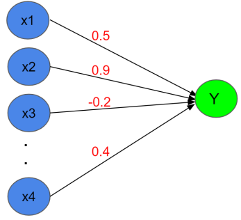
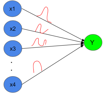
Figure 1: Traditional Neural Network (left) vs. Bayesian Neural Network (right).

II Related Work

In the quest to improve the adversarial robustness of neural networks, a few researchers adopt fusing Bayesian Inference with traditional NNs. Ye and Zhu [11] proposes BAL (Bayesian Adversarial Learning) to alleviate the shortcomings of traditional NNs. The posterior of the BNN is approximated with a scalable Markov Chain Monte Carlo sampling strategy, specifically stochastic gradient adaptive Hamiltonian Monte Carlo (SGAdaHMC) [11]. Thus to construct BAL, the BNN is trained with sampled adversarial examples and significantly outperforms all other defense models (i.e., adversarially trained traditional NNs). BAL is further improved by Adv-BNN, which is proposed by [8]. The posterior of this BNN is approximated with variational Bayes/Inference, specifically using a Gaussian distribution [8]. This BNN approach is trained with adversarial examples generated by $l_{\infty}$-PGD attack. [8, 11] show that adversarial training of BNNs further improves robustness and achieves state-of-the-art results in defending against adversarial attacks.

Another technique to improve a traditional NN involves using Kronecker factored Laplace to approximate the posterior of a NN [12]. When evaluated on white-box adversarial attacks, these BNN perform better at measuring uncertainty and are unlikely to make false predictions. Furthermore, the results suggest that it is less vulnerable to both targeted and non-targeted adversarial attacks [12]. Additionally, using 2 BNNs (i.e., Variational Inference and Hamilton Monte Carlo) trained on MNIST and attacked with $l_{\infty}$-FGSM and $l_{\infty}$-PGD attacks, BNNs are found to be robust to these attacks [13]. This work focuses on proving that BNNs should be robust to gradient-based attacks. Furthermore, [13] theoretically prove that gradient-based attacks in the thermodynamic limit are ineffective to BNNs.

Lastly, BNN’s ability to measure uncertainty well makes it robust to adversarial attacks [14, 15] due to the statistical guarantees leveraged by it’s ability to withstand adversarial attacks.

III Bayesian Neural Network

A Neural Network (NN) can be represented as a probabilistic model $p(y|x,w)$ such that $y$ is the set of classes and $p(y|x,w)$ is a categorical distribution. Given training dataset $D=\{x^{(i)},y^{(i)}\}$, we can obtain the weights $w$ of a NN by maximizing the likelihood function $p(D|w)=\prod_{i}p(y^{(i)}|x^{(i)},w)$. Maximizing the likelihood function gives us the MLE (Maximum Likelihood Estimate) of $w$. Thus, to transform a traditional Neural Network into a Bayesian Neural Network, we use Bayes theorem:

$$p(w|D)=\frac{p(D|w)p(w)}{p(D)}$$ (1)

to estimate the weights. $p(w|D)$ is the probability of the weights given the data. It is known as the posterior probability. $p(D|w)$ is the likelihood, $p(w)$ is the prior, and $p(D)$ is the evidence probability. Using bayes theorem, we can get a probability distribution that estimates the weights instead of single-point estimates gotten from MLE. But solving for $p(D)$ expands to a high dimensional integral, $p(D)=\int p(D,w)dw=\int p(w)p(D|w)dw$ [16]. This makes solving for an analytical solution of $p(w|D)$ intractable. Thus, an approximate function is needed to approximate the true posterior. Some of the techniques include Metropolis-Hastings, Hamilton Monte Carlo, Variational Inference, Etc. [17]. We will focus on variational Bayes/inference [18, 19, 20], the technique we employed because of its inexpensive computational cost and unbiased estimates it samples. Using the variational Bayes technique, a variational distribution $q(w|\theta)$ of known functional form is used to approximate the true posterior. This is achieved by minimizing the Kullblack-Leibler divergence between $q(w|\theta)$ and the true posterior $p(w|D)$ w.r.t. $\theta$, which is represented as $KL(q(w|\theta)~{}||~{}p(w|D))$. The KL-divergence can be expanded to:

$$F(D,\theta)=KL(q(w|\theta)~{}||~{}p(w))-\mathbb{E}_{q(w|\theta)}\log(p(w|D))$$ (2)

where,

$$KL(q(w|\theta)~{}||~{}p(w))=\int q(w|\theta)\log\frac{q(w|\theta)}{p(w)}dw$$

However, this too becomes intractable since finding an analytical solution for $KL(q(w|\theta)~{}||~{}p(w))$ is too computationally costly to solve in real-time. Therefore, to solve for the posterior, we can sample from the approximate function, $q(w|\theta)$. This is easier than sampling from the true posterior, $p(w|D)$. In doing so, we achieve a tractable function that can be written as:

$$F(D,\theta)\approx\frac{1}{N}\sum_{i=1}^{N}\big{[}\log q(w^{(i)}|\theta)-\log p(w^{(i)})-\log p(D|w^{(i)})\big{]}.$$ (3)

To sample $q(w|\theta)$, we model $\theta$ as a Gaussian distribution such that $\theta\sim\mathcal{N}(\mu,\sigma^{2})$, where $\mu$ and $\sigma^{2}$ are the mean and variance vectors of the distribution, respectively. Approximation of the true posterior using KL-divergence is also known as the ELBO (Evidence Lower BOund) method since the goal is to maximize the evidence lower bound [21]. See difference between Traditional NN and BNN in figure 1.

Lastly, training a BNN differs slightly from training a traditional NN. In traditional NNs, the weights and biases are calculated and updated with backpropagation. Since BNN has 2 parameters ($\mu$ and $\sigma^{2}$) to estimate the weights, the training process requires two parameters to be calculated and updated. This training process is is known as Bayes by Backprop [18].

IV Method

Since the ultimate goal is to build a model robust to adversarial attacks, specifically white-box attacks, we investigate the role of fusing Bayesian Inference with traditional NN. Previous work fused Bayesian Inference with VGG16 [8], and we hypothesize that we could build a more robust BNN by changing the backbone and making different parameter choices. VGG16 [22], while a powerful image classifier, does not possess some of the advantages of DenseNet [23], which makes it a robust classifier. These advantages include the use of densely connected layers to diversify features [24], reduction of parameters [24], and alleviation of the vanishing-gradient problem [25]. Therefore, we fuse Bayesian Inference with DenseNet121, creating BNN-DenseNet, making the backbone of our BNN, DenseNet. We choose DenseNet121 instead of other variants of DenseNet because it has fewer dense layers making it suitable for extracting learned concepts. Fusing Bayesian Inference with DenseNet121 means that the Convolutional and Batchnorm layers of DenseNet will no longer have single-point estimates, but a Gaussian distribution, $N(0_{d},\sigma^{2}I_{d\times d})$, to sample the posterior’s weights and biases. Therefore, weights are dependent on 2 parameters $w\sim\mathcal{N}(\mu,\sigma^{2})$ Furthermore, this essentially doubles NN parameters. The use of a Gaussian distributions of different sizes to estimate the weights and biases of the NN leads to the training of an ensemble of NNs.

We observe that the benefits of BNNs: (1) naturally regularizes; (2) does not overfit; (3) measures uncertainty well; (4) trains an ensemble of NNs. Therefore, we decide to further improve upon our BNN by training it with adversarial examples generated with $l_{\infty}$-PGD using $\epsilon=0.03$ and 10 iterations. Transforming BNN-DenseNet $\to$ BDAV is a two-fold problem - (1) generate adversarial data, $D^{adv}$ such that new data can fool classifier, and (2) learn from adversarial data, $D^{adv}$ such that predictions are reasonable. This leads to having a loss function that can capture the two-fold problem: (1) loss function for predicting the perturbed data and (2) generating the adversarial examples. Which can be written as:

$$L(D)=cross\_entropy+\beta\cdot KL\_loss,$$ (4)

where $\beta$ is a hyperparameter for balancing the cost of data generation. This is also known as the KL-divergence weight ($kl\_weight$).

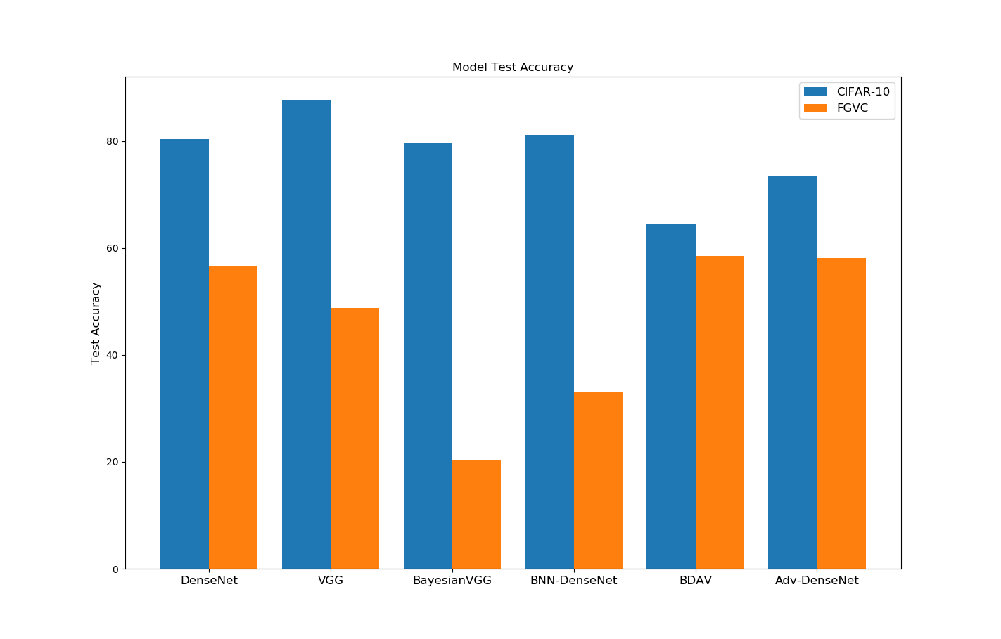
Figure 2: Test Accuracy of the 6 models trained on CIFAR-10 and FGVC datasets

V Experimental setup

V-A Data

For our experiments, we use benchmark datasets - CIFAR-10 [26] and FGVC-Aircraft (Fine-Grained Visualization Classification) [9] datasets. CIFAR-10 and FGVC are $32\times 32$ pixels and $224\times 224$ pixels, respectively. Thus, FGVC is the more non-trivial dataset with 10,000 Aircraft images. Furthermore, its labels are hierarchical, and it could be classified with 100 airplane models, 70 families, or 30 manufacturers as labels. For this task, we use the 30 manufacturers (i.e., Boeing, Airbus, Eurofighter, Etc.) labels to classify the dataset.

V-B Model Architecture

We use Adam optimizer for all the models except BayesianVGG, which used Stochastic Gradient Descent as its optimizer.

• DenseNet: We use DenseNet121 [27], a variant of DenseNet. The model was implemented using torchvision, a python package with the default parameters (i.e., # of input features are 32).

• VGG^∗: We use an off-the-shelf VGG16 [22] model from the PyTorch python package.

• BayesianVGG^∗: Obtained from Liu et al.’s implementation of fusing variational inference/Bayes with VGG16. The variance and mean were chosen to be $0.15$ each.

• BNN-DenseNet: This is our contribution. We use torchbnn, a python package to fuse Bayesian inference with DenseNet121. Previous experiments on DenseNet suggested robustness [28, 23], and thus fusing it with Bayesian inference improved the robustness even further. The variance and mean were chosen to be $0.15$ each.

• BDAV: This is also our contribution. BDAV is BNN-DenseNet trained with adversarial examples generated with $l_{\infty}$-PGD attack with 0.03 epsilon and 10 iterations. We use Adam optimizer, constant kl weight (0.1) and default parameters of DenseNet121 to train BDAV.

• Adv-DenseNet^∗: We train on DenseNet121 with adversarial examples generated by $l_{\infty}$-PGD attack with 0.03 epsilon and 10 iterations. This was to compare the robustness of adversarially trained traditional NNs vs. adversarially trained BNNs.

V-C White-Box Adversarial Attacks

We attacked our models with strong white-box attacks ($l_{\infty}$-FGSM, $l_{\infty}$-PGD, $l_{2}$-PGD, EOT $l_{\infty}$-FGSM, and EOT $l_{\infty}$-PGD), which are variants of:

• FGSM. This is a gradient-based attack introduced by [2]. Fast Gradient Sign Method (FGSM) works by applying perturbations in the direction of the gradient. This can be written as:

  $$x^{adv}=x+\epsilon\cdot sign(\nabla_{x}J(x,y_{target})),$$ (5)

  where $x$ is the clean image, $x^{adv}$ is the adversarially perturbed image, $J$ is the loss function, $y_{target}$ is the target/true label, and $\epsilon$ is the turnable parameter.

• PGD. This is another gradient-based attack introduced by [7]. Projected Gradient Descent (PGD) is an iterative variant of FGSM making it a stronger attack. This can be written as:

  $$x^{adv_{t+1}} =x^{adv_{t}}+\alpha\cdot sign(\nabla_{x}J(x^{adv_{t}},y_{target}))$$ (6)

  $$x^{adv_{t+1}} =\textbf{clip}(x^{adv_{t+1}},x^{adv_{t}}-\epsilon,x^{adv_{t}}+\epsilon)$$ (7)

  where $\textbf{clip}(.,a,b)$ function is in the range $[a,b]$.

• EOT. Athalye et al. [10] introduced the Expectation over Transformation (EOT) attack. EOT attack generates different image transformations, such that a slightly tilted image can fool the classifier. Unlike other attack methods, EOT keeps the distance between the clean and perturbed images in a threshold rather than minimize it [10]. The expected distance under transformation can be written as:

  $$\mathbb{E}_{t\sim T}[d(t(x^{adv}),t(x))],$$ (8)

  where $t(x)$ is the transformed clean image and $t(x^{adv})$ is the transformed adversarial image. The EOT optimizes the search for adversarial examples by maximizing the probability for the true class $y_{target}$ across all possible distributions of transformations T [29]. This is written as:

  $$\arg\max_{x^{adv}}\mathbb{E}_{t\sim T}[\log p(y_{target}|t(x^{adv}))]$$ (9)

  such that the expected distance over all possible transformations between $x$ and $x^{adv}$ is constrained at $\epsilon$, the threshold. This can be written as:

  $$\mathbb{E}_{t\sim T}[d(t(x^{adv}),t(x))]<\epsilon~{}~{}and~{}~{}x\in[0,1]^{d}.$$ (10)

  Thus, we investigate the performance of combining the EOT attack with the $l_{\infty}$ attacks. This implies that EOT transformed images perturb either $l_{\infty}$-FGSM or $l_{\infty}$-PGD attacks to improve the attacks’ strength further. Lastly, since the EOT attack is robust to models that incorporate randomness, we investigate our BNN models’ robustness to this attack.

All the $l_{\infty}$ attacks use epsilons in range $0-0.07$, while the $l_{2}$-PGD use epsilons $0-4$. We choose these epsilons because they increase the strength of the attacks. Thus, we attack our models with 10 and 40 iterations of the $l_{\infty}$-PGD and $l_{2}$-PGD attacks. We also test the model performance when we attack with 10-100 iterations of the $l_{\infty}$-PGD attack with $0.03$ epsilon. Lastly, we use 30 ensemble size and 40 iterations for the EOT attacks.

V-D Network Calibration analysis

Recent/modern NNs have achieved higher accuracies than NNs from past decades. However, while NNs have improved in classification and detection tasks, they have also become less well-calibrated [30]. A well-calibrated NN produces confidence output that matches the accuracy. For instance, if a NN achieves a 60% accuracy (i.e., 60% correct predictions), a well-calibrated model will also have achieved a 60% confidence score for each prediction. Thus, to further investigate our trained models’ robustness, we plot the accuracy’s output and confidence (probabilities of each class) into an identity function. Identifying how confident each model is in its prediction of clean data. These plots are also known as reliability diagrams [31, 30]. Furthermore, we use common calibration metrics - ECE (expected calibration error) and MCE (maximum calibration error) to evaluate these plots [30]. We adopt Guo et al.’s formal definitions of Accuracy, Confidence, ECE and MCE for this analysis. Lastly, we did not apply any calibration techniques to our model for this work since the aim is to observe which models require more or less calibration. Thus, we include confidence calibration measures as a robustness metric.

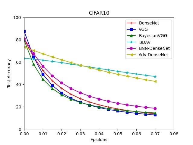
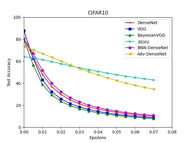
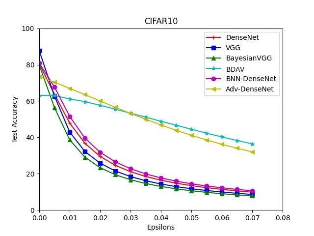
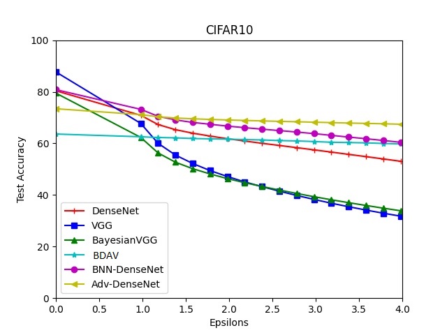
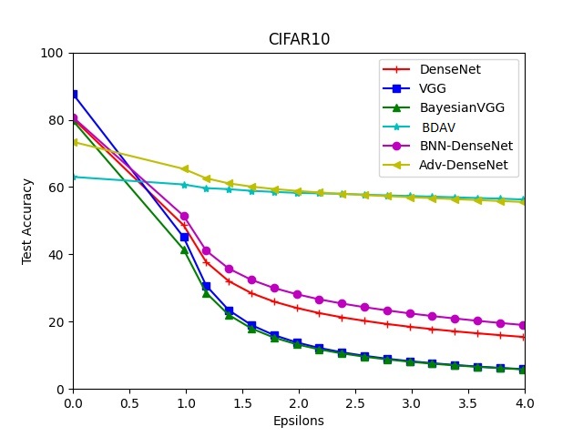
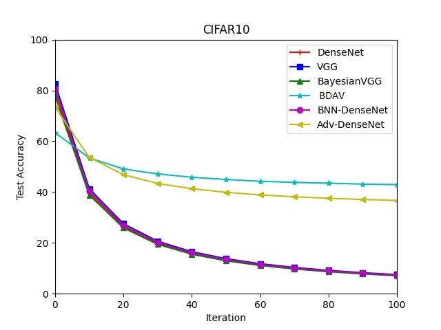
Figure 3: (Arranged from left-to-right) CIFAR10 trained models attacked with $l_{\infty}$-FGSM, 10 iterations $l_{\infty}$-PGD, 40 iterations $l_{\infty}$-PGD, 10 iterations $l_{2}$-PGD, 40 iterations $l_{2}$-PGD, and Iteration vs. Test Accuracy for $l_{\infty}$-PGD

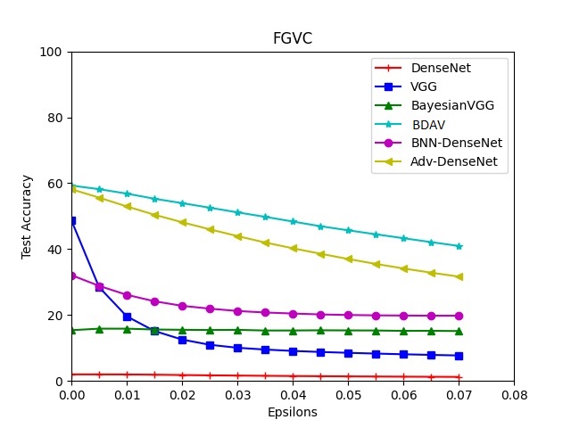
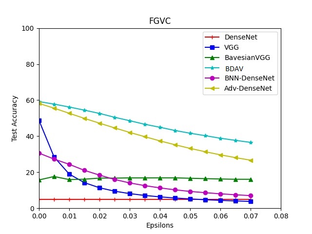
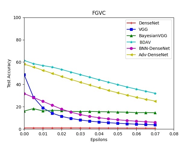
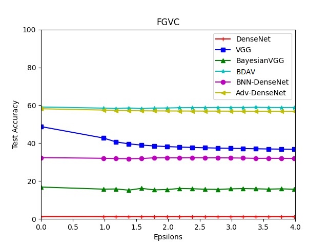
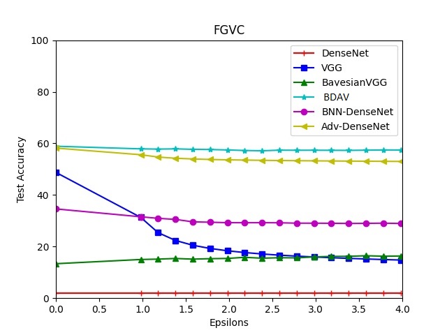
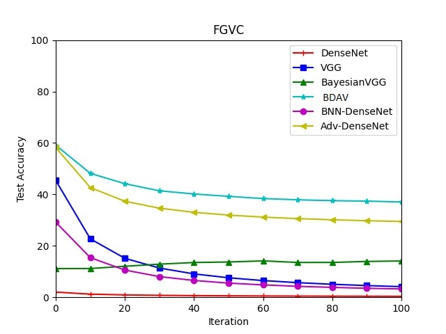
Figure 4: (Arranged from left-to-right) FGVC-Aircraft trained models attacked with $l_{\infty}$-FGSM, 10 iterations $l_{\infty}$-PGD, 40 iterations $l_{\infty}$-PGD, 10 iterations $l_{2}$-PGD, 40 iterations $l_{2}$-PGD, and Iteration vs. Test Accuracy for $l_{\infty}$-PGD

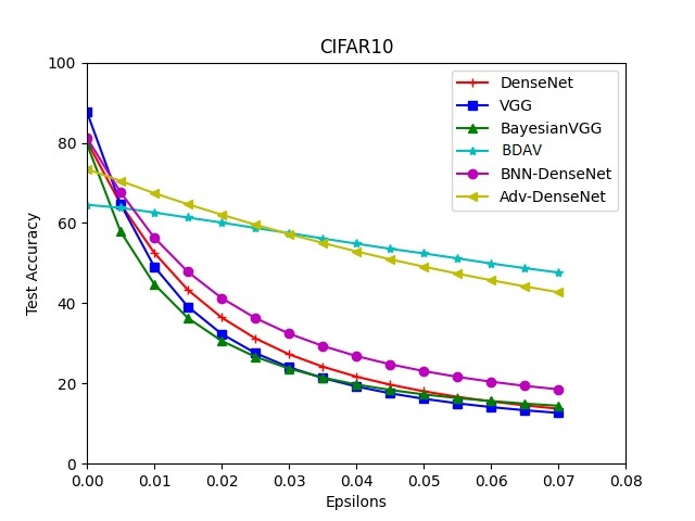
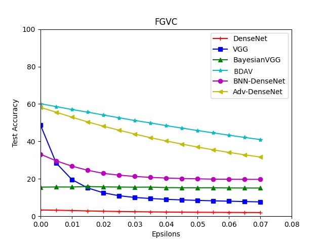
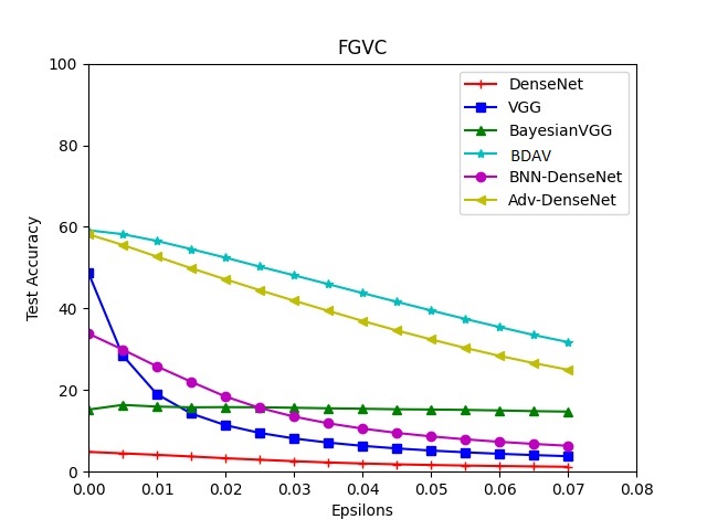
Figure 5: CIFAR-10 (top) and FGVC (bottom) trained models attacked with EOT $l_{\infty}$-FGSM and EOT $l_{\infty}$-PGD attacks with 30 ensemble size and 40 iterations

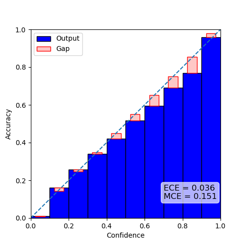
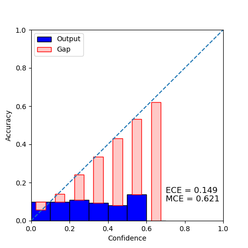
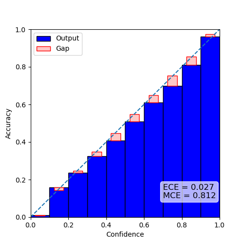
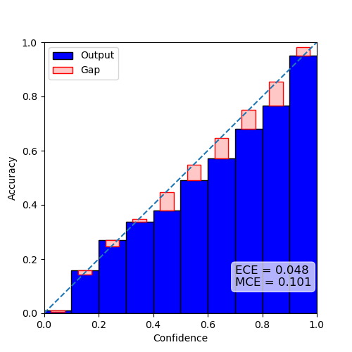
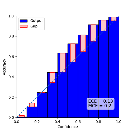
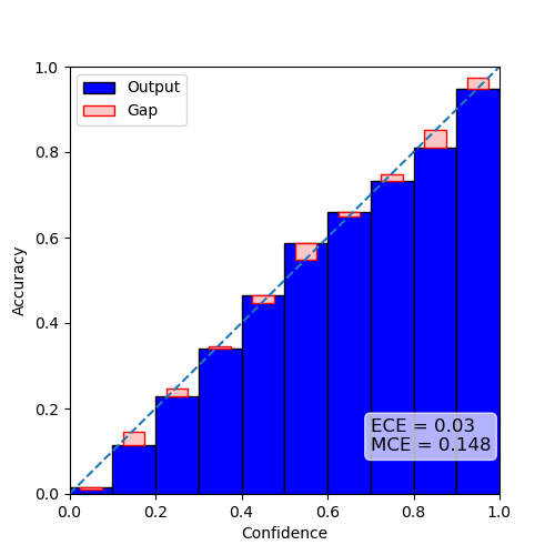
(a) CIFAR-10

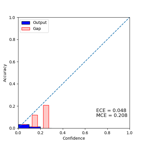
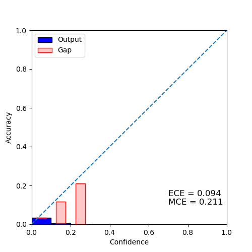
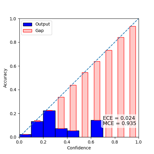
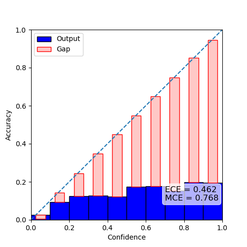
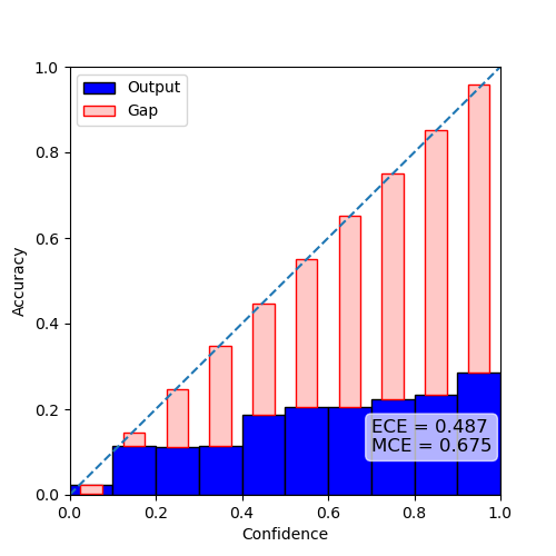
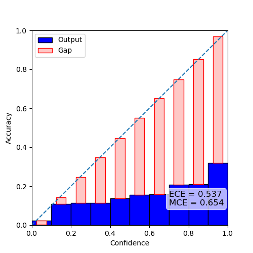
(b) FGVC

Figure 6: (Arranged from left-to-right) Network calibration plots of DenseNet, VGG, BayesianVGG, BNN-DenseNet, BDAV, and Adv-DenseNet.

VI Results

In this section, we compare the performance of the baseline models to BNN-DenseNet and BDAV. Using CIFAR-10 and FGVC datasets, we train these 6 models and obtain the following test accuracies in Figure 2. For CIFAR-10, VGG achieves the highest test accuracy (87.700%), and for FGVC, BDAV achieves the highest accuracy (58.566%).

We attack our trained models with strong state-of-the-art white-box adversarial attacks. See Figures 3 and 4 for the performance of models trained on CIFAR-10 and FGVC attacked with $l_{\infty}$-FGSM, $l_{\infty}$-PGD, and $l_{2}$-PGD, respectively. The figures are results of the following attacks: $l_{\infty}$-FGSM, 10 iterations of $l_{\infty}$-PGD, 40 iterations of $l_{\infty}$-PGD, 10 iterations of $l_{2}$-PGD, 40 iterations of $l_{2}$-PGD, and Iteration (between 0-100) vs. Test Accuracy for $l_{\infty}$-PGD with $\epsilon=0.03$, respectively. We also attacked our models with EOT $l_{\infty}$-FGSM and EOT $l_{\infty}$-PGD attacks using 30 ensemble size and 40 iterations. See Figure 5 for plotted results of the models attacked with EOT attacks.

Then, to further investigate the robustness of these models, we perform a network calibration analysis. We plot the accuracy’s output and confidence (probabilities of each class) into an identity function to evaluate each model’s quality of the predictions. Using 10 bins, we can see the difference between the model confidence and accuracy. See figure 6 for network calibration plots.

Lastly, we observe that the computational cost of the EOT attacks are high. The EOT $l_{\infty}$-PGD was especially expensive, taking about 10 days to attack CIFAR-10 and 53 days to attack FGVC.

VII Discussion

The selection of a particular dataset can make a model seem robust. This can be seen in Figures 3, 4 and 5, where traditional NNs (VGG and DenseNet) perform reasonably on CIFAR-10 but underperform on FGVC. Therefore, to properly ascertain the robustness of a model, we find that training on complex data can be beneficial in extracting concepts.

Furthermore, we observe that BNN-DenseNet outperforms the traditional NNs and BayesianVGG in Figure 3. This suggest that BNNs are more robust to adversarial attacks than traditional NNs. We also observe that BDAV outperforms Adv-DenseNet. What is most interesting here is that the two models intersect in performance at $\epsilon=0.03$. It is at this point that BDAV starts to outperform Adv-DenseNet. However, in the case of FGVC, the performance of the BNNs are even more exaggerated. We see that in Figure 3 that for all attacks except for $l_{2}$-PGD with 10 iterations, a BNN model (BNN-DenseNet or BayesianVGG), outperforms all the traditional NNs, significantly. Also, BDAV outperforms Adv-DenseNet in this scenario significantly as well. Therefore, the results suggest that since BDAV decays linearly at a slow rate when attacked with strong epsilons, it is much more able to withstand white-box adversarial attacks than other models.

Additionally, to further evaluate the BNN models’ robustness to adversarial attacks that incorporate randomization, we attack our trained models with EOT attacks. We find that for CIFAR-10, the difference between the naive attacks and EOT are relatively the same. This may be due to the dataset, not the model, because we observe a very different performance on models trained on FGVC. We see that our BNN models are more robust than traditional NNs in this attack scenario. Since BNN is a model that incorporates randomization, it is robust but should be susceptible to stochastic attacks in nature. However, we find that the opposite holds true as our BNN models are robust to the EOT attacks. The reason for this behavior could be because BNNs operate under a mathematically justifiable principle. Using Bayesian Inference provides many benefits, such as the promotion of a stable stochastic model. Furthermore, it is important to consider the computational cost of EOT attacks, especially the EOT $l_{\infty}$-PGD attack.

Lastly, robustness for this work is defined as a model’s ability to be insusceptible or have a low susceptibility to strong adversarial attacks and make accurate predictions (i.e., confidence and accuracy should match). Therefore, we investigate our 6 models’ calibration and find that BNN-DenseNet and BayesianVGG require less calibration than the other models. We also see that these BNN models make less overconfident predictions and are therefore less likely to be fooled by adversarial perturbations of images. Additionally, since there is no free lunch, the incorporation of adversarial training to a BNN also has disadvantages. This can be seen in Figure 6, where BDAV is seen as a bit overconfident and at times having a slightly higher ECE and/or MCE than Adv-DenseNet while BNN-DenseNet is almost well-calibrated.

VIII Conclusion

Since the traditional framework of deep learning or neural network models are susceptible to adversarial attacks, we claim that this vulnerability is as a result of the shortcomings of the models. These shortcomings include - overconfidence, being data greedy, the need for regularization, and a huge potential to overfit. These disadvantages appear because deep learning models/traditional NNs do not measure for uncertainty well. Therefore we claim that incorporating an uncertainty measure will mitigate these shortcomings and as an added bonus, improve the robustness. This is achieved by fusing Bayesian Inference with a traditional NN (DenseNet121). The dense nature of DenseNet121, provides advantages that are amplified when fused with Bayesian Inference. Then to further improve BNN-DenseNet, we incorporate adversarial training to the model and construct BDAV.

We compare these two models’ performance to 4 baseline models - 2 traditional NN, a BNN, and adversarially trained NN. Then, we attack our models with 5 different strong state-of-the-art white-box attacks - $l_{\infty}$-FGSM, $l_{\infty}$-PGD, $l_{2}$-PGD, EOT $l_{\infty}$-FGSM, and EOT $l_{\infty}$-PGD. To further evaluate robustness, we also performed a network calibration analysis of our models to ascertain which models were closer to being well-calibrated without incorporating any calibration techniques. We find that the BNNs are more robust than the traditional NNs. Also, incorporating adversarial training to a BNN improves the robustness even further. However, while it improves the BNN’s robustness to adversarial attacks, there appears to be a cost. This is seen in Figure 6, where BNN-DenseNet is closer to being well-calibrated than BDAV. We also observe that BNN-DenseNet has a lower ECE than BDAV.

In the future, we will explore benefits of calibrating BDAV to improve test accuracy and robustness. We will also investigate the effect of using different approximation functions, like MCMC on adversarial robustness.

References

- Szegedy et al. [2013] C. Szegedy, W. Zaremba, I. Sutskever, J. Bruna, D. Erhan, I. Goodfellow, and R. Fergus, “Intriguing properties of neural networks,” arXiv preprint arXiv:1312.6199, 2013.
- Goodfellow et al. [2014] I. J. Goodfellow, J. Shlens, and C. Szegedy, “Explaining and harnessing adversarial examples,” arXiv preprint arXiv:1412.6572, 2014.
- Fawzi et al. [2018] A. Fawzi, H. Fawzi, and O. Fawzi, “Adversarial vulnerability for any classifier,” in Advances in neural information processing systems, 2018, pp. 1178–1187.
- Nguyen et al. [2015] A. Nguyen, J. Yosinski, and J. Clune, “Deep neural networks are easily fooled: High confidence predictions for unrecognizable images,” in Proceedings of the IEEE conference on computer vision and pattern recognition, 2015, pp. 427–436.
- Shukla et al. [2020] S. N. Shukla, M. P. Vadera, B. Jalaian, and B. M. Marlin, “Adversarial distillation of bayesian neural networks,” 2020.
- Hernández-Lobato and Adams [2015] J. M. Hernández-Lobato and R. Adams, “Probabilistic backpropagation for scalable learning of bayesian neural networks,” in ICML, 2015, pp. 1861–1869.
- Madry et al. [2018] A. Madry, A. Makelov, L. Schmidt, D. Tsipras, and A. Vladu, “Towards deep learning models resistant to adversarial attacks,” in ICLR, 2018.
- Liu et al. [2018] X. Liu, Y. Li, C. Wu, and C.-J. Hsieh, “Adv-bnn: Improved adversarial defense through robust bayesian neural network,” in International Conference on Learning Representations, 2018.
- Maji et al. [2013] S. Maji, J. Kannala, E. Rahtu, M. Blaschko, and A. Vedaldi, “Fine-grained visual classification of aircraft,” Tech. Rep., 2013.
- Athalye et al. [2018] A. Athalye, L. Engstrom, A. Ilyas, and K. Kwok, “Synthesizing robust adversarial examples,” in ICML. PMLR, 2018, pp. 284–293.
- Ye and Zhu [2018] N. Ye and Z. Zhu, “Bayesian adversarial learning,” in Proceedings of the 32nd International Conference on Neural Information Processing Systems, 2018, pp. 6892–6901.
- Ritter et al. [2018] H. Ritter, A. Botev, and D. Barber, “A scalable laplace approximation for neural networks,” in 6th International Conference on Learning Representations, ICLR 2018-Conference Track Proceedings, vol. 6. International Conference on Representation Learning, 2018.
- Carbone et al. [2020] G. Carbone, M. Wicker, L. Laurenti, A. Patane, L. Bortolussi, and G. Sanguinetti, “Robustness of bayesian neural networks to gradient-based attacks,” NeurIPS, 2020.
- Cardelli et al. [2019] L. Cardelli, M. Kwiatkowska, L. Laurenti, N. Paoletti, A. Patane, and M. Wicker, “Statistical guarantees for the robustness of bayesian neural networks,” IJCAI, 2019.
- Smith and Gal [2018] L. Smith and Y. Gal, “Understanding measures of uncertainty for adversarial example detection,” arXiv preprint arXiv:1803.08533, 2018.
- Blei et al. [2017] D. M. Blei, A. Kucukelbir, and J. D. McAuliffe, “Variational inference: A review for statisticians,” Journal of the American statistical Association, vol. 112, no. 518, pp. 859–877, 2017.
- Mullachery et al. [2018] V. Mullachery, A. Khera, and A. Husain, “Bayesian neural networks,” arXiv preprint arXiv:1801.07710, 2018.
- Blundell et al. [2015] C. Blundell, J. Cornebise, K. Kavukcuoglu, and D. Wierstra, “Weight uncertainty in neural network,” in International Conference on Machine Learning, 2015, pp. 1613–1622.
- Hinton and Van Camp [1993] G. E. Hinton and D. Van Camp, “Keeping the neural networks simple by minimizing the description length of the weights,” in Proceedings of the sixth annual conference on Computational learning theory, 1993, pp. 5–13.
- Graves [2011] A. Graves, “Practical variational inference for neural networks,” in Advances in neural information processing systems, 2011, pp. 2348–2356.
- Zhang et al. [2018] G. Zhang, S. Sun, D. Duvenaud, and R. Grosse, “Noisy natural gradient as variational inference,” in International Conference on Machine Learning, 2018, pp. 5852–5861.
- Simonyan and Zisserman [2014] K. Simonyan and A. Zisserman, “Very deep convolutional networks for large-scale image recognition,” arXiv preprint arXiv:1409.1556, 2014.
- Li and Vu [2018] C. Y. Li and N. T. Vu, “Densely connected convolutional networks for speech recognition,” in Speech Communication; 13th ITG-Symposium. VDE, 2018, pp. 1–5.
- Zhu and Newsam [2017] Y. Zhu and S. Newsam, “Densenet for dense flow,” in 2017 IEEE international conference on image processing (ICIP). IEEE, 2017, pp. 790–794.
- Jégou et al. [2017] S. Jégou, M. Drozdzal, D. Vazquez, A. Romero, and Y. Bengio, “The one hundred layers tiramisu: Fully convolutional densenets for semantic segmentation,” in Proceedings of the IEEE conference on computer vision and pattern recognition workshops, 2017, pp. 11–19.
- Krizhevsky [2009] A. Krizhevsky, “Learning multiple layers of features from tiny images,” 2009.
- Huang et al. [2017] G. Huang, Z. Liu, L. Van Der Maaten, and K. Q. Weinberger, “Densely connected convolutional networks,” in Proceedings of the IEEE conference on computer vision and pattern recognition, 2017, pp. 4700–4708.
- Jang and Park [2019] D.-W. Jang and R.-H. Park, “Densenet with deep residual channel-attention blocks for single image super resolution,” in Proceedings of the IEEE Conference on Computer Vision and Pattern Recognition Workshops, 2019, pp. 0–0.
- Molnar [2020] C. Molnar, Interpretable Machine Learning. Lulu. com, 2020.
- Guo et al. [2017] C. Guo, G. Pleiss, Y. Sun, and K. Q. Weinberger, “On calibration of modern neural networks,” in ICML, 2017, pp. 1321–1330.
- Niculescu-Mizil and Caruana [2005] A. Niculescu-Mizil and R. Caruana, “Predicting good probabilities with supervised learning,” in Proceedings of the 22nd international conference on Machine learning, 2005, pp. 625–632.