Fitting XMM-Newton Observations of the AXP 1RXS J170849.0$-$400910 with four magnetar surface emission models, and predictions for X-ray polarization observations with IXPE

Abstract

Context. Phase-resolved spectral and spectropolarimetric X-ray observations of magnetars present us with the opportunity to test models of the origin of the X-ray emission from these objects, and to constrain the properties of the neutron star surface and atmosphere.

Aims. Our first aim is to use archival XMM-Newton observations of the magnetar 1RXS J170849.0$-$400910 to ascertain how well four emission models describe the phase-resolved XMM-Newton energy spectra. Our second aim is to evaluate the scientific potential of future spectropolarimetric observations of 1RXS J170849.0$-$400910 with the Imaging X-ray Polarimetry Explorer (IXPE) scheduled for launch in late 2021. The most salient questions are whether IXPE is able to distinguish between the different emission models, and whether IXPE can unambiguously detect the signatures of quantum electrodynamics (QED) effects in strong magnetic fields.

Methods. We used numerical radiation transport calculations for a large number of different system parameters to predict the X-ray flux and polarization energy spectra of the source 1RXS J170849.0$-$400910. Based on the numerical results, we developed a new model to fit phase-resolved and phase-averaged X-ray spectral (i.e., XMM-Newton and IXPE) and spectropolarimetric (IXPE) data. In order to test the sensitivity of IXPE to strong-field QED effects, we fit a simulated IXPE observation with two versions of the model, i.e., with and without QED effects accounted for.

Results. The fixed-ions condensed surface model gives the best description of the phase-resolved XMM-Newton spectra, followed by the blackbody and free-ions condensed surface models. The magnetized atmosphere model gives a poor description of the data and seems to be largely excluded. Simulations show that the IXPE observations of sources such as 1RXS J170849.0$-$400910 will allow us to cleanly distinguish between high-polarization (blackbody, magnetized atmosphere) and low-polarization (condensed surface) models. If the blackbody or magnetized atmosphere models apply, IXPE can easily prove QED effects based on $\sim$200 ksec observations as studied here; longer IXPE observation times will be needed for a clear detection in the case of the condensed surface models.

Conclusions. The XMM-Newton data have such a good signal-to-noise ratio that they reveal some limitations of the theoretical models. Notwithstanding this caveat, the fits clearly favor the fixed-ions condensed surface and blackbody models over the free-ions condensed surface and magnetized atmosphere models. The IXPE polarization information will greatly help us to figure out how to improve the models. The first detection of strong-field QED effects in the signal from astrophysical sources seems possible if an adequate amount of time is dedicated to the observations.

1 Introduction

Magnetars are peculiar, isolated neutron stars (NSs) believed to host the strongest magnetic fields among astrophysical sources. Although historically they have been classified into two distinct classes, the anomalous X-ray pulsars (AXPs) and the soft-gamma repeaters (SGRs), they share quite similar observational properties, including measured spin periods $P$ in the $\sim 2$–$12$ s range, and period derivatives $\dot{P}$ in the $10^{-13}$–$10^{-11}$ s/s range. Within the usual magneto-dipolar braking scenario, these values imply ultra-strong magnetic fields of up to $B\approx 10^{14}$–$10^{15}$ G, which is orders of magnitude greater than those derived in conventional rotation-powered pulsars.

Both AXPs and SGRs are observed to emit powerful bursts and flares in hard X-rays and in soft-$\gamma$ rays with peak luminosities ranging from $10^{36}$ erg/s for the weaker and more frequent short bursts, and up to $10^{47}$ erg/s for the rarest and most powerful giant flares (detected only from three SGRs up to now, see Mazets et al., 1979; Hurley et al., 1999; Palmer et al., 2005). The persistent emission in the $2$–$10$ keV band, $L_{X}\approx 10^{31}$– $10^{36}$ erg/s (typically in excess of the rotational energy loss rate), is well fit by the superposition of a blackbody component ($kT\approx 0.5$–$1$ keV) and a nonthermal, power-law tail, with photon index $\Gamma\approx 2$–$4$, although a purely thermal spectrum is observed in some (mostly transient) sources. An additional power-law has been detected from several sources at higher energies ($\gtrsim 20$ keV, see Mereghetti, 2008; Turolla et al., 2015; Kaspi & Beloborodov, 2017, for reviews).

The most successful scenario in explaining the phenomenology of magnetars is the so-called twisted magnetosphere model Duncan & Thompson (1992); Thompson et al. (2002). According to this model, the internal magnetic field of the star is characterized by a nonnegligible toroidal component, which is able to exert strong magnetic stresses on the conductive crust and displaces surface elements to which the external magnetic field lines are anchored. As a consequence, the external dipole field becomes “twisted”, that is it acquires a sizable toroidal component. The presence of such a toroidal component makes the external field nonpotential so that charged particles must flow along the closed field lines. The situation thus differs from the case of conventional pulsars, where currents flow only along the open field lines Goldreich & Julian (1969). The presence of charges makes the (inner) magnetosphere optically-thick to resonant Compton scattering (RCS). Comptonization of (thermal) radiation emitted by the NS surface results in the formation of the power-law tail emission observed in the soft X-ray band Thompson et al. (2002); Nobili et al. (2008); Zane et al. (2009). Moreover, the plastic deformations of the crust caused by the internal magnetic stresses may be also responsible for the emission of short bursts and flares, through the injection in the magnetosphere of an electron-positron fireball which eventually remains trapped within the closed field line region Thompson & Duncan (1995, 2001); Taverna & Turolla (2017).

For sources with ultra-strong magnetic fields, such as magnetars, the polarization state of the photons cannot be neglected. In these strong fields, photons propagate in two linearly polarized normal modes: in the ordinary (O) mode, with the electric field oscillating in the plane of the local magnetic field $\boldsymbol{B}$ and the propagation direction $\boldsymbol{k}$; and in the extraordinary (X) mode, with the electric field oscillating perpendicularly to both $\boldsymbol{k}$ and $\boldsymbol{B}$ (see e.g., Ginzburg, 1970; Gnedin & Pavlov, 1974). In such a strongly magnetized medium, the properties of the radiative processes and opacities depend strongly on the polarization state. The absorption of extraordinary photons for example is strongly suppressed outside the resonance Pavlov & Panov (1976); Herold (1979); Ventura (1979), leading to a high polarization degree of the RCS-reprocessed surface emission. The observed polarization fractions depend strongly on geometrical effects, which tend to depolarize the signal. For magnetic field strengths close to or exceeding $B_{\rm q}\simeq 4.4\times 10^{13}$ G QED effects play a role. The QED effects however tend to preserve the intrinsic polarization fraction (see e.g., Heyl et al., 2003; Taverna et al., 2014, 2015).

The spectral shape and polarization properties of the persistent magnetar emission depend on the physical state of the neutron stellar surface. The state of the surface is still a debated issue and no unanimous consensus has been reached as of yet. In one model, a geometrically-thin/optically-thick atmosphere covers the surface of the star (e.g., Romani, 1987; Shibanov et al., 1992; Pavlov et al., 2004; Zavlin et al., 1996; Lai & Salpeter, 1997; Lai, 2001). However, for field strengths and temperatures typical of magnetar sources, the surface layers may be in a condensed state Ruderman (1971); Lai & Salpeter (1997); Turolla et al. (2004), which would result in a “bare”, solid surface, so that surface emission is directly injected into the magnetosphere. While X-ray spectral observations can test some predictions of these models, the spectral information alone is not sufficient to identify the emission model, as they tend to predict similar thermal energy spectra. The models however predict very different polarization properties (see e.g., Suleimanov et al., 2009; Potekhin et al., 2012; Taverna et al., 2020). As a consequence, X-ray polarimetry can definitely probe the nature of magnetar surface layers.

For these reasons, magnetars are among the primary targets of the Imaging X-ray Polarimetry Explorer IXPE mission scheduled for launch in 2021 Weisskopf et al. (2016) as well as the eXTP mission Zhang et al. (2019). The polarimetric observations will probe the emission mechanism, and will provide new independent constraints on the geometry of the source, removing degeneracies which affect spectral analyses. Furthermore, the observations will allow us to observe the effect of vacuum birefringence, a strong-field QED prediction Heyl et al. (2003); Taverna et al. (2015); González Caniulef et al. (2016); Taverna et al. (2020).

In this paper we focus on the AXP 1RXS J170849.0$-$400910 Israel et al. (1999). The source is one of the brightest (persistent) magnetar sources (see the McGill online magnetar catalog, Olausen & Kaspi, 2014) and is among the highest-priority targets to be observed in the first year of the IXPE science mission. We first compare the energy spectra predicted by the magnetar emission models of Taverna et al. (2020) with archival XMM-Newton observations of this source (see Rea et al., 2008; Zane et al., 2009). We perform for the first time not only a phase-averaged analysis, but also a phase-resolved analysis. For the best-fit models, we present simulated IXPE observations, and show how well IXPE can distinguish between these emission models. Our analysis indicates that the combined spectral and polarization data will allow us to identify the emission model, and to constrain the source geometry and QED effects. After introducing the theoretical framework in Sect.  2, we summarize the numerical implementation in Sect.  3. We discuss the implementation of the model as a fitting model in Sect.  4. Sect.  5 discusses the results from fitting the XMM-Newton observations of 1RXS J170849.0$-$400910. Sect.  6 demonstrates what IXPE will add to our studies of magnetars, by presenting the analysis of simulated IXPE observations. We close with a discussion of the results in Sect.  7.

Table 1: Parameters of the magnetar model.

Parameter Name	Description	Units	Allowable Range
model	1 (blackbody), 2 (magnetized atmosphere), 3 (fixed-ions condensed surface), 4 (free-ions condensed surface)	-	1-4
norm	overall normalization	-	0 … inf
chi	inclination from rotation axis	$[^{\circ}]$	0.1 … 89.9
xi	angle between rotation and magnetic axes	$[^{\circ}]$	0.1 … 89.9
deltaPhi	magnetic field line twist angle	[rad]	0.3 … 1.4
beta	electron bulk velocity	$[c]$	0.2 … 0.7
phi	anticlockwise rotation to celestial north pole	$[^{\circ}]$	0 … 180
phaseResolved	1 (0) for phase-resolved (phase-averaged) analysis	-	0, 1
offset	offset added to the model phase (phase-resolved analysis only)	-	0. … 1.
dir	+1 (-1) for pulse evolution as modeled (inverted) (phase-resolved analysis only)	-	-1, 1
phase1	start of interval for averaging (phase-averaged analysis only)	-	0 … 1
phase2	end of phase interval for averaging, a value smaller than phase1 will result in averaging the model from phase2 to phase1 (phase-averaged analysis only)	-	0 … 1

2 Theoretical framework

2.1 Magnetospheric structure

In this and the following sections, we recall the most important underlying assumptions we used in our work to produce the model archive for fitting the observational and simulated data. In the framework of the twisted magnetosphere model Thompson et al. (2002), the amount of shear of the external magnetic field is usually described through the so-called twist angle $\Delta\phi$, which measures the angular displacement between the footpoints of a given field line. Although the twist is more likely restricted to localized bundles of field lines Thompson et al. (2002); Beloborodov (2009), we assumed for the sake of simplicity that the external dipolar field is globally twisted: namely, all the external field lines are sheared by the same amount $\Delta\phi_{\rm N-S}$, maintaining the global axial symmetry (Taverna et al., 2014, see also Nobili et al. 2008; Fernández & Davis 2011).We stress that the magnetic field topology surrounding an ultra-magnetized NS is likely to be much more complicated than that of a (twisted) dipole. Small-scale magnetic flux tubes may rise close to the star surface, as suggested, for example, by the detection of a phase-dependent (proton) cyclotron line in the X-ray spectrum of SGR 0418-5729 Tiengo et al. (2013). However, multipolar components decay much faster with increasing distance from the star than the dipole component. Given that resonant scatterings mostly occur at about $10\,{R_{\rm NS}}$ (Thompson et al., 2002; Nobili et al., 2008), only the dipole component of the field survives in the region of interest.

Under these conditions, the polar components of the star magnetic field can be expressed as

$$\boldsymbol{B}=\frac{{B_{\rm p}}}{2}\left(\frac{r}{{R_{\rm NS}}}\right)^{-p-2}\left[-\frac{{\rm d}{f}}{{\rm d}\cos\theta},\frac{pf}{\sin\theta},\sqrt{\frac{Cp}{p+1}}\frac{f^{1+1/p}}{\sin\theta}\right]\,,$$ (1)

where ${B_{\rm p}}$ is the polar magnetic field strength, ${R_{\rm NS}}$ the star radius and $f$ is a function of the magnetic colatitude $\theta$, obtained as a solution of the Grad-Shafranov equation (see Thompson et al., 2002; Pavan et al., 2009). The radial index $p$ and the parameter $C$ are related to the twist angle $\Delta\phi_{\rm N-S}$ by

$$\Delta\phi_{\rm N-S}=\sqrt{\frac{C}{p(p+1)}}\lim_{\theta\rightarrow 0}\int_{\theta}^{\pi/2}\frac{f^{1/p}}{\sin\theta}{\rm d}\theta\,.$$ (2)

Since $C$ is an eigenvalue of the problem, it is completely determined once $p$ is assigned. This implies that the globally twisted field is fixed once ${B_{\rm p}}$ and $p$, or equivalently $\Delta\phi_{\rm N-S}$, are provided. The latter option is adopted in this paper.

It has been shown that the magnetospheric currents, which must stream along the closed field lines due to the additional toroidal component in the external field, should be sustained mainly by electron-positron pairs Beloborodov & Thompson (2007). However, since a detailed model which accounts for pairs has not yet been developed, we consider the simplified scenario in which the charge carriers are electrons and ions extracted from the crust due to the strong surface magnetic field Fernández & Thompson (2007); Nobili et al. (2008); Fernández & Davis (2011); Taverna et al. (2014). Ions, however, are lifted at much smaller heights above the surface (as they are much heavier than electrons) and they are expected to contribute less to the emerging photon spectrum than electrons (see Thompson et al., 2002, for a detailed analysis). Following these considerations, we adopt the uni-directional flow approximation, in which only electrons are considered to stream along the closed field lines. In our simulations, we described the motion of these magnetospheric electrons as a bulk motion (from the northern to the southern magnetic hemisphere) at constant velocity $\beta$ in units of the speed of light. Moreover, in order to account for the velocity spread, we superimposed a (relativistic) Maxwellian distribution at the temperature $T_{\rm e}$, which is one-dimensional because of the magnetic confinement which affects electrons perpendicularly to the $B$-field (see also Nobili et al., 2008, for more details), to the bulk motion. Clearly, the assumption of constant bulk velocity is an oversimplification. Charges accelerate after they are extracted from the star surface, reach a maximum velocity, and then decelerate as they hit the outermost layers. This was discussed by Beloborodov & Thompson (2007) in connection with a simplified, but more realistic, model in which pair creation is accounted for. Again, much as in the case of the dipole field assumption, we are mostly concerned with what happens at about ten star radii, far from the initial or terminal parts of the charge trajectory. In this respect taking the electron velocity to be a constant is not entirely unrealistic. Under these assumptions, the density of magnetospheric particles can be expressed in terms of the magnetic field strength and the twist parameter as Thompson et al. (2002); Nobili et al. (2008)

$$n_{\rm e}=\frac{p+1}{4\pi e}\frac{B}{\beta r}\left(\frac{B_{\phi}}{B_{\theta}}\right)\,,$$ (3)

where $e$ is the electron charge. This value turns out to be sufficiently high to make the medium optically thick for RCS. As the photon energy $E$ reaches in the particle rest frame the electron cyclotron energy $\omega_{\rm ce}=\hbar eB/m_{\rm e}c\simeq 11.6\,(B/10^{12}\,{\rm G})$ keV (with $m_{\rm e}$ the electron mass), the photon is absorbed by the electron, which is in turn excited to its first Landau level. The particle de-excitation, however, occurs in a very short time ($\approx 3\times 10^{-14}\,(B/10^{11}\,{\rm G})^{-2}\,{\rm s}$, see e.g. Fernández & Davis, 2011) and a photon is emitted at the same energy, so that the process is akin to a scattering event in all respects. In the case of magnetars, with surface radiation emitted at $E\approx 1$ keV and $B_{\rm p}\sim 10^{14}$ G, the resonance condition is met as the magnetic field strength has dropped down to $\sim 10^{11}$ G, which occurs at about $5$–$10\,{R_{\rm NS}}$. Due to RCS, thermal photons emitted from the stellar surface are expected to be up-scattered by magnetospheric electrons, populating the nonthermal tail in the soft X-ray spectra ($0.1$–$10$ keV) of these sources (see e.g. Mereghetti, 2008; Rea & Esposito, 2011; Turolla et al., 2015; Kaspi & Beloborodov, 2017, for reviews).

Table 2: Results from fitting the XMM-Newton EPIC-pn data with the four phase and angle averaged absorbed emission models.

Model Name	$\chi^{2}$/DoF	norm	$\Delta\phi$	$\beta$	$n_{\rm H}$
		[$10^{-8}$]	[rad]	[$c$]	[$10^{22}{\rm cm}^{-2}$]
Blackbody	1122.8/67	12.3	0.30	0.30	0.494
Magnetized atmosphere	39239/67	4.9	0.30	0.20	0.537
Free-ions cond. surf.	2372.6/67	10.2	0.30	0.34	0.471
Fixed-ions cond. surf.	858.85/67	9.4	0.30	0.33	0.295

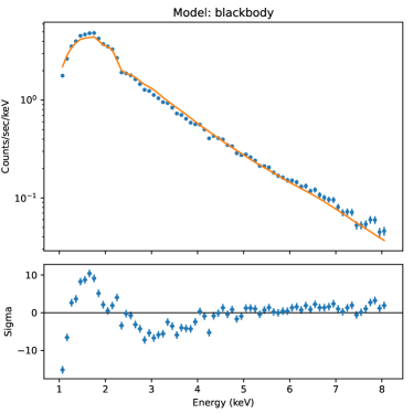
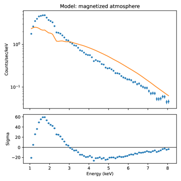
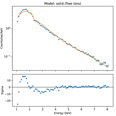
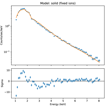
Figure 1: Best-fit models of the phase-averaged XMM-Newton data (upper panels, blue data points) with the phase and angle averaged models (upper panels, orange lines). The lower panels show (data-model)/sigma for the spectra shown above.

2.2 Photon polarization transport

In the strong field limit the cross sections which describe the interactions between photons and charged particles can be dramatically different with respect to the unmagnetized ones, and they change according to the photon polarization state. Strong magnetic fields have a strong impact on the polarization dependent cross sections of radiative processes such as Compton scattering (or even second-order processes such as free-free emission and photon splitting, see Lieu, 1981; Lauer et al., 1983; Stoneham, 1979; Bulik, 1998), and the scatterings are more strongly suppressed for X-mode photons than for O-mode ones Lai et al. (2010). RCS is not an exception; photons originally polarized in the O-mode that resonantly scatter off electrons may change their polarization state into the X-mode and vice versa as given by the RCS cross sections Thompson et al. (2002); Nobili et al. (2008); Taverna et al. (2014):

$$\begin{array}[]{lll}\sigma_{\rm O-X}&=&3\sigma_{\rm O-O}\\ &&\\ \sigma_{\rm X-O}&=&\dfrac{1}{3}\sigma_{\rm X-X}\,.\end{array}$$ (4)

Equations (4) imply that photons emerging from the magnetosphere are preferentially polarized in the extraordinary mode, with a typical ratio of 3:1 with respect to those emerging in the ordinary mode.

Table 3: Results from fitting the XMM-Newton EPIC-pn data with the four phase-resolved absorbed magnetar emission models.

Model Name	$\chi^{2}$/DoF	norm	$\chi$	$\xi$	$\Delta\phi$	$\beta$	$n_{\rm H}$	offset
		[$10^{-9}$]	[∘]	[∘]	[rad]	[$c$]	[$10^{22}{\rm cm}^{-2}$]
Blackbody	3372.5/703	12.6	0.1	0.1	0.40	0.47	0.610	0.864
Blackbody†	3419.4/703	12.1	15	60	0.30	0.40	0.556	0.860
Magnetized atmosphere	37432.5/703	6.14	15.0	0.1	0.30	0.20	0.	0.856
Free-ions cond. surf.	3728.9/703	9.16	0.1	87	0.30	0.39	0.335	0.864
Fixed-ions cond. surf.	3103.9/703	8.74	15	60	0.50	0.35	0.513	0.858

^† Fit with $\chi$ and $\xi$ tied to the best-fit values of the fixed-ions condensed surface model.

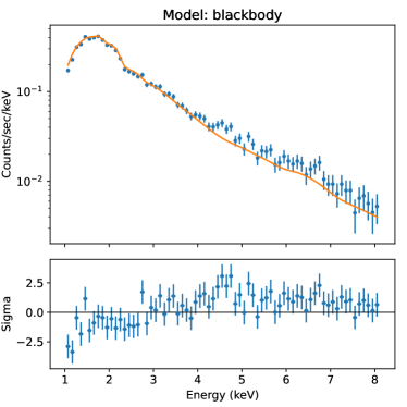
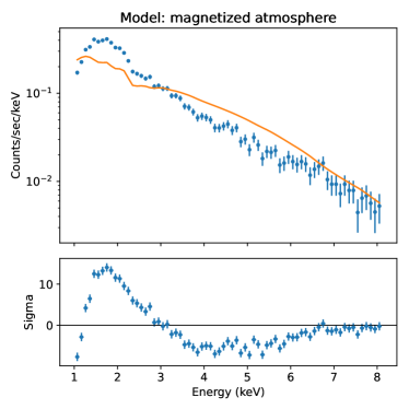
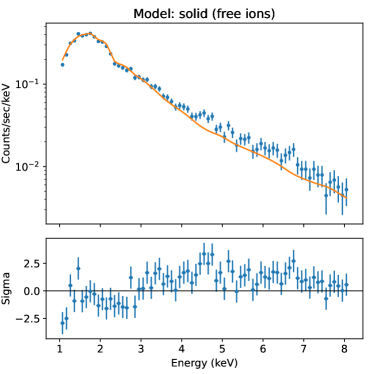
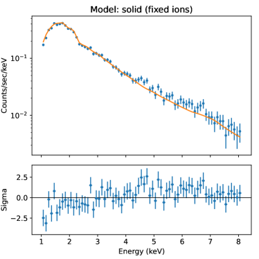
Figure 2: Exemplary spectra of the XMM-Newton data for phase bin 3 (upper panels, blue data points) and models (upper panels, orange line), that is blackbody model (top left), magnetized atmosphere model (top right), free-ions condensed surface (bottom left), and fixed-ions condensed surface (bottom right). The lower panels show (data-model)/sigma for the spectra above.

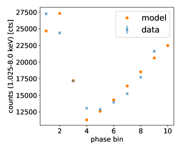
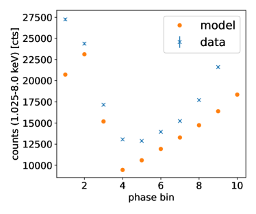
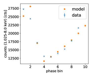
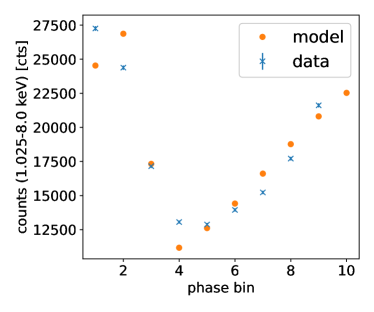
Figure 3: Observed (blue crosses) and theoretical (orange circles) 0.5-8 keV pulse diagrams of the best-fit blackbody model (top left), magnetized atmosphere model (top right), free-ions condensed surface (bottom left), and fixed-ions condensed surface (bottom right). The XMM-Newton data are shown with error bars which are so small that they cannot be seen for most data points.

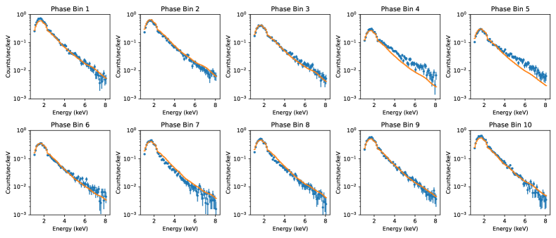
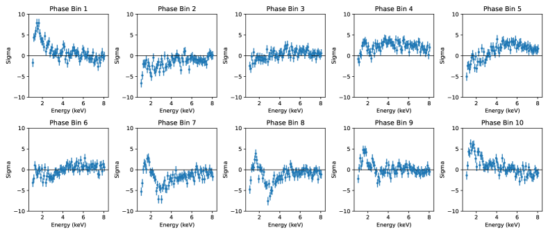
Figure 4: Upper panels: XMM-Newton data of all ten phase-resolved spectra (blue data points) and the best-fit model (fixed-ions condensed surface, orange lines). Lower panels: deviation ((data-model)/sigma) for all spectra.

In the case of magnetars, however, photon polarization states can be also modified as they propagate in vacuo due to vacuum polarization, a QED effect originally theorized by Heisenberg & Euler (1936) and independently by Weisskopf (1936). Ultra-strong magnetic fields (typically in excess of the quantum critical field $B_{\rm q}\simeq 4.4\times 10^{13}$ G) can polarize the virtual electron-positron pairs which populate the magnetized vacuum around the star. As a consequence, the components of both the dielectric and magnetic permeability tensors of vacuum deviate from unity, ensuring that O- and X-mode photons propagate with slightly different refraction indices (vacuum birefringence). In order to understand how QED effects can influence the polarization properties of the emitted radiation, one should solve the wave equation, accounting for the vacuum polarization terms. It turns out that, close to the surface, the strong magnetic field of the star can force the photon polarization vector to maintain its original orientation relative to the magnetic field direction (adiabatic propagation), which in turn can vary along the photon trajectory. Hence, the polarization pattern of the emitted radiation is practically unchanged until the star magnetic field becomes too weak to affect the photon polarization states. This typically occurs at a distance $r_{\rm pl}$ from the star, called the polarization-limiting radius (see Heyl et al., 2003; Taverna et al., 2015),

$$r_{\rm pl}\simeq 4.8\left(\frac{B_{\rm p}}{10^{11}\,{\rm G}}\right)^{2/5}\left(\frac{E}{1\,{\rm keV}}\right)^{1/5}\left(\frac{{R_{\rm NS}}}{10\,{\rm km}}\right)^{1/5}\,{R_{\rm NS}}\,.$$ (5)

This radius increases with the magneic field strength. As the photons move outward, the polarization vectors freeze. The photon polarization states can deviate from the initial ones if the magnetic field direction still changes substantially along the photon trajectory. As a consequence of these effects, stronger magnetic fields lead to polarization signatures that are closer to those at emission, allowing us to probe the physical processes at the surface and in the inner magnetosphere through polarimetric measurements (see e.g., Taverna et al., 2015; González Caniulef et al., 2016).

Finally, another important effect may take place when plasma contributions to the dielectric tensor become comparable to those of vacuum polarization (the so-called vacuum resonance, see Lai & Ho, 2002, 2003). This occurs at a density

$$\rho_{\rm V}\simeq 0.964Y_{\rm e}^{-1}\left(\frac{E}{1\,{\rm keV}}\right)^{2}\left(\frac{B}{10^{14}\,{\rm G}}\right)^{2}\zeta^{-2}\,{\rm g\,cm^{-3}}\,,$$ (6)

where $Y_{\rm e}$ is the plasma electron fraction and $\zeta$ is a slowing varying function of the magnetic field strength. In these conditions photon polarization modes can switch from O to X and vice versa, with a probability

$$P_{\rm con}=1-\exp\left[-\frac{\pi}{2}\left(\frac{E}{E_{\rm ad}}\right)^{3}\right]\,,$$ (7)

where $E_{\rm ad}$ is the energy at which mode conversion occurs.

2.3 Surface emission models

As described in Taverna et al. (2020), we consider three different models to predict the spectral and polarization properties. In the first model, photons are emitted directly from the stellar surface following a blackbody distribution and they are assumed to be 100% polarized in the extraordinary mode. In the second model, photons are reprocessed in an optically-thick, geometrically-thin magnetized atmosphere that covers the stellar surface. Finally, in the third model, emission occurs from the “bare”, solid surface of the star, which is assumed to be composed by a magnetic condensate. For ease of reading, we briefly summarize in the following the main properties of each emission model, referring the reader to Taverna et al. (2020) for more details.

2.3.1 Blackbody model

The currently available soft X-ray spectra of many AXPs and SGRs can be fit well with the superposition of a thermal (blackbody) component and a nonthermal power law tail (see Mereghetti, 2008; Turolla et al., 2015, for reviews). The power-law component can be identified with photons, resonantly up-scattered by magnetospheric electrons (see e.g., Thompson et al., 2002; Fernández & Thompson, 2007; Nobili et al., 2008, compare Sect.  2.1). The thermal component can be associated with the cooling emission from the stellar surface. Following these observational findings, we make the zero-order approximation to describe photons from the stellar surface as blackbody emission at the temperature inferred from the observed spectra (that is $T\approx 0.5$ keV for our template source). As illustrated in section 2.2, the ultra-strong surface magnetic field of the star is expected to strongly affect the polarization pattern of the emitted radiation, favoring the propagation of extraordinary photons with respect to ordinary ones. On the other hand, some models predict that thermal O-mode photons are more likely emitted from hot-spots on the surface where magnetospheric currents return, which are more concentrated in the (magnetic) equatorial regions (see Thompson et al., 2002; Beloborodov & Thompson, 2007; Fernández & Davis, 2011). A self-consistent model that includes the effects of returning currents has not yet been developed. We thus make the simplified assumption that the blackbody emission is 100% polarized in the extraordinary mode.

2.3.2 Magnetized atmosphere

The presence of a magnetized atmospheric layer (with typical scale-height $0.1$–$10$ cm) above the surface of ordinary pulsars and even highly-magnetized isolated NSs has been suggested by many authors (see e.g., Lai & Salpeter, 1997; Lai, 2001; Zavlin & Pavlov, 2002) and different models have been developed to describe the radiation emitted from such atmospheres, both in the magnetized ($B\ga 10^{12}$ G) and in the nonmagnetized limits (see Suleimanov et al., 2009, for a complete list of references). However, model atmospheres around passively cooling NSs, which are in thermal and hydrostatic equilibrium, might not apply to active magnetars because the structure of such an atmosphere would be strongly affected by the bombardment of returning charged particles flowing along the closed field lines. Despite recent attempts to investigate the properties of such bombarded atmospheric layers (see Gonzàlez Caniulef et al., 2019), a complete understanding of the emitted spectrum and polarization is still lacking. With the aim to provide a more physically motivated emission model alongside the 100% polarized blackbody model mentioned above, we consider a simple plane-parallel magnetized atmosphere and use the radiation transfer code of Suleimanov et al. (2009) to characterize the energy spectrum and polarization properties of the emitted radiation. The code solves the radiative transfer equation for the ordinary and the extraordinary photons in the case of a partially ionized, pure hydrogen atmosphere using the opacities described in Potekhin et al. (2014). The polarization properties of the emitted radiation are then computed self-consistently from the O-mode and X-mode specific intensities (see Taverna et al., 2020, for more details). In this respect, we remark that the mode conversion induced by the vacuum resonance (see Sect.  2.2) is taken into account as discussed in Lai & Ho 2003, see also .

2.3.3 Condensed surface

For values of the magnetic field strength in excess of $\sim 2.4\times 10^{9}$ G such that the electron gyro-radius is comparable to the Bohr radius, the properties of matter are strongly modified. In particular, due to the confinement in the direction perpendicular to the magnetic field, the atomic electron clouds are squeezed in the direction of $\boldsymbol{B}$ and, for temperatures below a value $T_{\rm crit}$ (that depends on the composition, see Lai, 2001; Medin & Lai, 2007), molecular chains can be formed via covalent bonding. Under these conditions, a phase transition occurs (the so-called magnetic condensation, Ruderman, 1971; Lai & Salpeter, 1997), and the stellar surface turns into a “naked” solid surface Turolla et al. (2004). Considering the values of the surface temperature and the spin-down magnetic field strength inferred from observations Israel et al. (1999), it turns out that magnetic condensation is indeed a plausible scenario for 1RXS J170849.0$-$400910 (see for example Fig.  1 in Taverna et al., 2020). In order to reproduce the spectral and polarization properties of the emitted radiation in this case, we resort to the approximate fitting formulae developed by Potekhin et al. (2012, see also , for more details), that compute the emissivities for ordinary and extraordinary photons for a selected chemical composition (we adopted a Fe condensed surface). In our simulations we provide results in the two limits of (i) free-ions, that is ions on the stellar surface are free to move in response to the electromagnetic waves, and (ii) fixed-ions, with ions considered as fixed in a lattice. As stated in previous works (see e.g., van Adelsberg et al., 2005), the real situation should probably lie in between these two limits. We finally remark that, much in the same way as in the blackbody and in the magnetized atmosphere cases, we neglect the effects of returning currents in the condensed surface model as well.

3 Numerical implementation

As described in Taverna et al. (2020), we produced a number of different simulations using the Monte Carlo code originally developed by Nobili et al. (2008) with the addition of a specific module to account for photon polarization properties (see Taverna et al., 2014). The code starts by dividing the stellar surface into a number of equal-area patches, each labeled by the magnetic colatitude $\theta$ and azimuth $\phi$ of its center. Seed photons are launched randomly from each of these patches, according to the selected emission model. This can easily be achieved for the blackbody model using a series expansion method (see e.g., Barnett & Canfield, 1970). In the case of the magnetized atmosphere and condensed surface models, we use an acceptance/rejection method von Neumann (1951); Press et al. (1992). A similar sampling method is used to determine the polarization state of the emitted photons. The number $N_{\theta,\phi}$ of seed photons which are launched from each surface patch is determined by setting a reference number $\bar{N}$ for the patch which emits the smallest number of photons and weighing the photons of all the other patches according to the considered emission model. In our calculations, we chose a $\theta\times\phi=10\times 10$ angular mesh for the blackbody and the condensed surface models, and a $20\times 10$ angular mesh for the magnetized atmosphere model, choosing $\bar{N}$ in such a way that the total number of photons launched from the surface is $\sim 10^{7}$ for all the emission models. Photons are eventually collected on a $15\times 15$ angular mesh on the sky at infinity.

The code follows each photon along its trajectory and accounts for the resonant scatterings off magnetospheric electrons. In the adiabatic region close to the stellar surface, vacuum polarization effects are properly considered by locking the polarization mode to that set at emission or to the polarization mode resulting after each scattering. The wave equation is then solved for the photon Stokes parameters $I$, $Q$, $U$ and $V$ in the region between the RCS last scattering radius $r_{\rm esc}$ and the polarization limiting radius $r_{\rm pl}$ (see Taverna et al., 2014, 2020, for more details). We neglect strong gravity effects such as relativistic ray-bending to save computational resources, which allows us to run the simulations for each emission model in $\approx 5$ days on a single-CPU computer. We remark, however, that the effects of relativistic ray-bending should be small, as scatterings occur at a large distances from the star (see Sect.  2.1), where general relativistic effects are weak. Strong gravity effects do not play a major role for the polarization state of photons propagating around magnetars. In fact, the typical length scales along which the photon polarization vectors rotate due to strong-field QED effects (see Sect. 2.2) are much smaller than those relevant for general relativistic effects (see Connors & Stark, 1977; Stark & Connors, 1977; Connors et al., 1980).

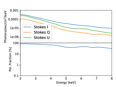
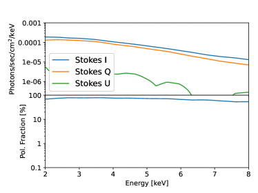
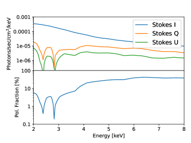
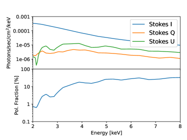
Figure 5: Absolute value of Stokes I, Q and U parameters (top panels) and linear polarization fraction (lower panels) for the blackbody model (top left), magnetized atmosphere model (top right), free-ions condensed surface (bottom left), and fixed-ions condensed surface (bottom right). For all models, the results for phase bin 3 are shown.

We run the Monte Carlo code assuming a fixed value of the polar magnetic field strength ${B_{\rm p}}=5\times 10^{14}$ G, which is compatible with 1RXS J170849.0$-$400910 and with many of the known AXPs and SGRs. For all the emission models, we assume a constant 0.5 keV surface temperature (see Taverna et al., 2020, for a complete discussion on this choice). We simulate twist angles $\Delta\phi_{\rm N-S}$ and charge bulk velocities $\beta$ between $0.3$–$1.4$ rad (step size: $0.1$ rad) and $0.2$–$0.7$ (step size: $0.1$), respectively. We added the value $\beta=0.34$ to the grid, corresponding to the electron bulk velocity obtained from the spectral fitting by Zane et al. (2009). We assume the same electron temperature $T_{\rm el}=10$ keV for all cases. Each single run is post-processed with an idl script to derive the energy spectra seen by an observer at infinity for different values of the two angles $\chi$ and $\xi$, which measure the inclination of the line-of sight and of the magnetic axis wrt the star rotation axis, respectively. The outputs of this script consist in one ascii file for each value of $\chi$, $\xi$, $\Delta\phi_{\rm N-S}$ and $\beta$. $\chi$ and $\xi$ range between $0$–$180^{\circ}$ (step $15^{\circ}$) and $0$–$90^{\circ}$ (step $15^{\circ}$), respectively. Each output file contains the Stokes parameters $I$, $Q/I$ and $U/I$ as functions of the photon energy (sampled by a 49-bin grid between $0.5$ and $10$ keV) and the rotational phase (sampled by a 9-bin grid between $0$ and $2\pi$).

4 Loading the model in sherpa

The spectral analysis is based on fitting the observed and simulated $I$ (XMM-Newton and IXPE) and $Q$ and $U$ (IXPE) energy spectra with a least squares technique based on the forward folding method Kislat et al. (2015); Strohmayer (2017); Krawczynski (2021). We used the kerrC model developed for fitting the spectropolarimetric observations of black holes as a template to develop a new model, called magnetar, to work with the data tables described above. The model uses the spectral fitting package sherpa, the general purpose fitting model developed as part of the CIAO Chandra analysis software (Freeman et al., 2001; Doe et al., 2007). The fitting module is written in Python 3.7 and uses the astropy library for saving and storing the predicted Stokes parameter $I$, $Q$, and $U$ energy spectra in the fits format, the numpy library for fast manipulation of the spectral data, and the scipy library for the interpolation between simulated parameter values using the regularGridinterpolation tool.

Table 4: Results from fitting the simulated IXPE blackbody data.

Model Name	$\chi^{2}$/DoF	norm	$\chi$	$\xi$	$\Delta\phi$	$\beta$	$n_{\rm H}$	$\phi$	offset
		[$10^{-9}$]	[∘]	[∘]	[rad]	[$c$]	[$10^{22}{\rm cm}^{-2}$]	[∘]
Blackbody (input)	NA	12.1	15.0	60.0	0.30	0.40	0.556	0	0.860
Blackbody (best fit)	195.0/202	12.1	15.7	59.8	0.33	0.37	0.557	-1.7	0.860
Fixed-ions cond. surf. (best fit)	754.6/202	9.26	15.7	60.0	0.30	0.44	0.642	1.1	0.919
Blackbody (no QED)	711.3/202	12.2	15.7	59.8	0.33	0.37	0.557	-1.7	0.860

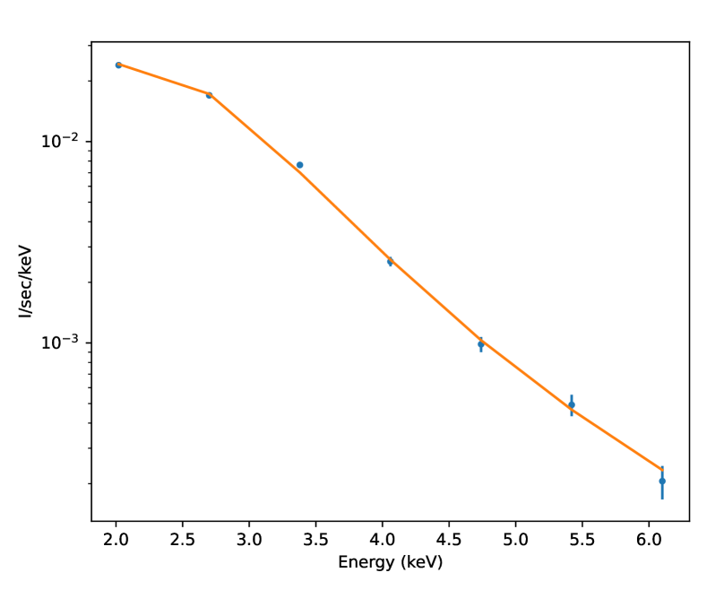
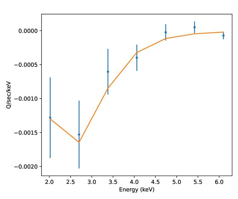
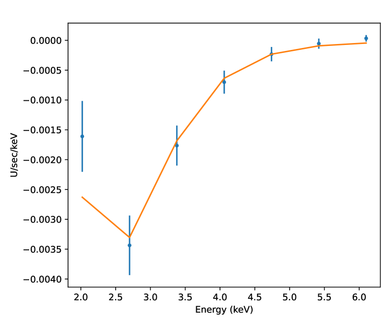
Figure 6: Simulated 200 ksec IXPE observations of AXP 1RXS J170849.0$-$400910 for the blackbody model showing the Stokes I (top), Stokes Q (center) and Stokes U (bottom) energy spectra for phase bin 3. The blue data points are the simulated IXPE data, and the orange lines are the best-fit model. For all ten phase bins, the fit gives a $\chi^{2}$ of 195.0 for 202 DoF.

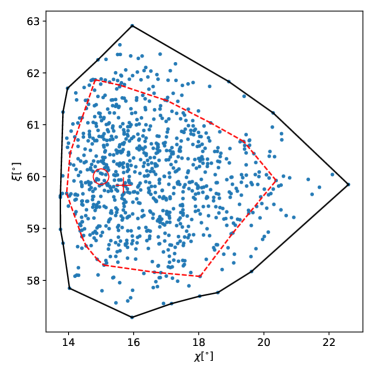
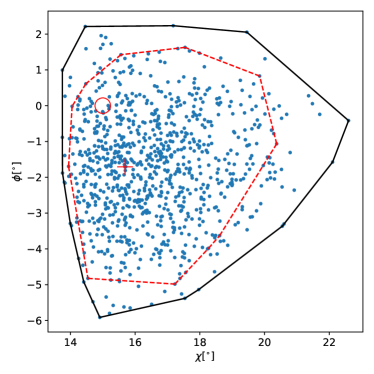
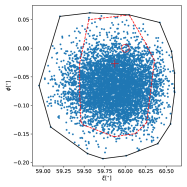
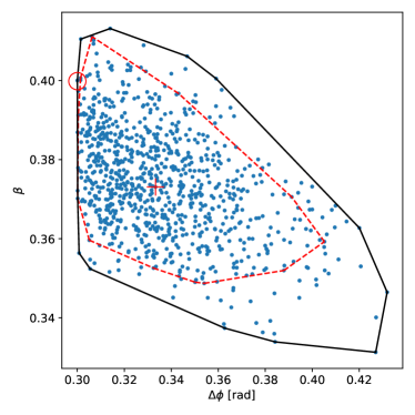
Figure 7: Contour plots of the spectral parameters obtained fitting the IXPE data for the case of the blackbody model. The red circles show the value for which the data set was simulated and the red crosses show the best-fit value. The red and black lines show the $\Delta\chi^{2}<13.36$ and $\Delta\chi^{2}<20.1$ contours, roughly corresponding to 90% and 99% confidence intervals.

Table 5: Results from fitting the simulated IXPE fixed-ions condensed surface data.

Model Name	$\chi^{2}$/DoF	norm	$\chi$	$\xi$	$\Delta\phi$	$\beta$	$n_{\rm H}$	$\phi$	offset
		[$10^{-9}$]	[∘]	[∘]	[rad]	[$c$]	[$10^{22}{\rm cm}^{-2}$]	[∘]
Fixed-ions cond. surf. (input)	NA	8.74	15.0	60.0	0.50	0.35	0.513	0.0	0.858
Blackbody (best fit)	435.6/202	12.2	9.8	58.5	0.73	0.20	0.212	16.6	0.861
Fixed-ions cond. surf. (best fit)	192.3/202	8.81	16.0	65.0	0.61	0.29	0.435	-1.1	0.855
Fixed-ions cond. surf. (no QED)	193.4/202	8.77	20.5	62.5	0.54	0.30	0.504	14.0	0.856

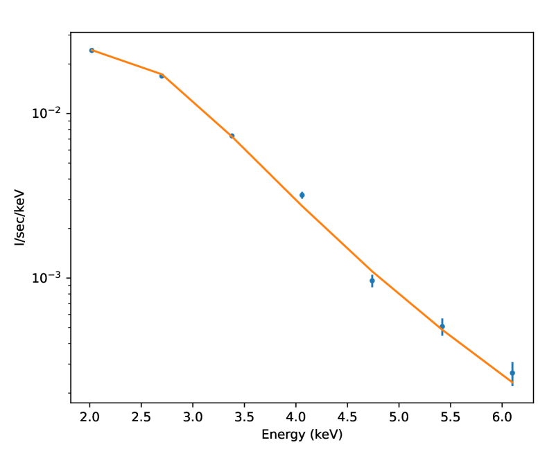
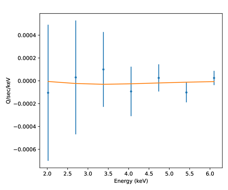
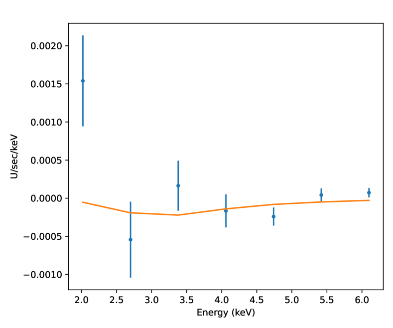
Figure 8: Simulated IXPE observations of AXP 1RXS J170849.0$-$400910 assuming the best-fit fixed-ions model that fits the actual XMM-Newton data. The blue data points show the simulated IXPE observations, and the orange lines show the best fit model that gives a $\chi^{2}$ of 192.3 for 202 DoF.

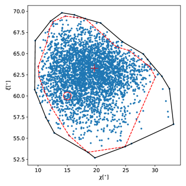
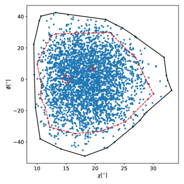
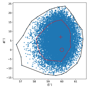
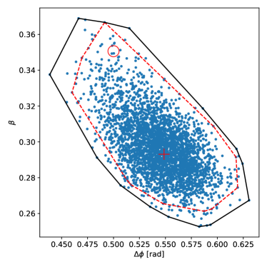
Figure 9: Contour plots of the spectral parameters obtained fitting the IXPE data for the case of the fixed-ions condensed surface model. The red circles show the value for which the data set was simulated and the red crosses show the best-fit value. The red and black lines show the $\Delta\chi^{2}<13.36$ and $\Delta\chi^{2}<20.1$ contours, roughly corresponding to 90% and 99% confidence intervals. .

For each detected or simulated event, a set of Stokes parameters is calculated:

$$i = 1$$ (8)

$$q = 2\cos{(2\psi)}$$ (9)

$$u = 2\sin{(2\psi)}\$$ (10)

with $\psi$ being the angle of the electric field vector measured counterclockwise from the celestial north pole. The “observed” $I_{\rm obs}$, $Q_{\rm obs}$ and $U_{\rm obs}$ energy spectra are obtained by summing the Stokes parameters of the individual events in $N$ energy bins. The factors of two in the expressions of $q$ and $u$ are chosen such that the measured values $I_{\rm obs}$, $Q_{\rm obs}$ and $U_{\rm obs}$ equal the Stokes $I$, $Q$, and $U$ values describing the X-ray beam Kislat et al. (2015).

We developed a python code to simulate and fit IXPE magnetar observations. The simulations use the Ancillary Response Function (ARF), the Redistribution Matrix File (RMF), and the Modulation Response Files (MRF) from Baldini (2020). Whereas the ARF gives the effective area of the telescope as a function of the photon energy (the product of the mirror area, blanket and other transmissivities, and the detector efficiency), the MRF is the product of the ARF and the energy dependent modulation factor $\mu(E)$. The latter gives the fractional modulation of the azimuthal scattering angle distribution for a 100% polarized signal and depends on the polarimeter, and the event reconstruction methods.

Based on the theoretically expected $I$, $Q$ and $U$ values, the code simulates the observed $I_{\rm obs}$, $Q_{\rm obs}$, and $U_{\rm obs}$ values with the help of the IXPE ARF, RMF, and MRF, taking the $Q$ and $U$ variances and the $Q-U$ covariances into account Kislat et al. (2015). We note that the modulation factor reduces the expected values of $Q_{\rm obs}$ and $U_{\rm obs}$ to $\mu$ times the Stokes $Q$ and $U$ values of the X-ray beam, The $\chi^{2}$-value is calculated using $\sqrt{I}$ as the error on $I_{\rm obs}$, and $\sqrt{2\,I}$ as the error on the $Q_{\rm obs}$ and $U_{\rm obs}$-values (Strohmayer, 2017).

Table 1 summarizes all the fitting parameters of the magnetar model. In addition to the model parameters mentioned above, the model includes several additional parameters. The model predictions can be scaled with an overall normalization factor norm. The polarization direction depends on the orientation of the source in the sky. Accordingly, the model includes the parameter $\phi$ to rotate the simulated source anticlockwise relative to the celestial north pole. The model allows the user to perform a phase-averaged or a phase-resolved analysis. In the case of the former, the user specifies the phase interval over which the model is averaged. In the case of the latter, the user specifies two additional parameters: a phase offset offset and the phase direction dir. The value offset instructs the code to fit the data at phase $x$ with the model at phase $x+$offset. A value of dir=+1 uses the simulated phase sequence as modeled, and a value of dir=-1 inverts the order of the modeled sequence (inverted phase $=$ 1-phase). The inverted phase corresponds to the emission of a magnetar with mirror-imaged geometry. We use the sherpa’s levmar and moncar minimization engines. We find that sherpa fits the phase-resolved XMM-Newton data relatively quickly and reliably. The fits of the simulated IXPE data converge more slowly and often end up in local minima. We address this issue by starting the fit from many different initial parameter values, and choosing the fit result with the overall lowest $\chi^{2}$-value. Once the latter is found, we initiate a random exploration of 50,000 parameter combinations in the $\sim\pm$3$\sigma$ neighborhood of the best-fit parameter combination. This random exploration is used to map out the $\chi^{2}$ test statistics and thus the confidence intervals on the parameters, and to double check that the search indeed found the minimum of the test statistic. If the random exploration reveals a parameter configuration with a lower test statistics, the random walk is recentered on the new minimum.

5 Results from fitting the XMM-Newton observations

The XMM-Newton data were acquired between 21:50:40 UTC on August 28, 2003 and 10:11:51 UTC on August 29 with a total exposure time of 44.7 ksec (obs. ID 0148690101). We use here only the data from the EPIC-pn camera, that was operated in small-window mode with the medium thickness optical filter. The data reduction was performed using the epproc and espfilt pipelines of version 15 of the Science Analysis System (SAS), with standard parameters. We corrected the time of arrivals to the Solar System barycenter with the tool barycen, and then we folded them to the best fitting period of 11.00178(2) s. The source events and the ARF and RMF were selected from a circle of radius 27” centered on the source position, while the background was extracted from a nearby circular region of radius 40”. We obtained the spectra corresponding to 10 phase bins, and we rebinned them using the grppha tool with a minimum of 30 counts per bin.

The results from fitting the XMM-Newton data with the phase and angle averaged magnetar models are shown in Table 2 and Fig.  1. The blackbody, free-ions condensed surface, and fixed-ions condensed surface models give the best fits with $\chi^{2}/$Degrees of Freedom (DOF)-values of 1123/67, 2373/67 and 859/67, respectively. The magnetized atmosphere models gives a much poorer fit with a $\chi^{2}/$DoF-values of 39239/67. The poor fit of the magnetized atmosphere model is a recurring finding of the analyses shown in this paper. The magnetized atmosphere model predicts a thermal component that is too broad.

The results from fitting the phase-resolved XMM-Newton data with the phase and angle resolved magnetar model are shown in Table 3. The fixed-ions condensed surface model gives the best fit ($\chi^{2}$/degree of freedom (DoF) $=$ 3103.9/703) followed by the blackbody model ($\chi^{2}$/DoF $=$ 3372.5/703) and the free-ions condensed surface model ($\chi^{2}$/DoF $=$ 3728.9/703). Compared with the other ones, the magnetized atmosphere gives by far the poorest fit, with a $\chi^{2}$/DoF-values of 37432.5/703. For all models, the fit strongly prefers the inverted pulse sequence (dir$=$-1), indicating that the geometry of AXP 1RXS J170849.0$-$400910 is the mirror image of the one assumed in our model. As this result is consistent across all considered models, we do not mention it any more in the following. For the blackbody model, we repeated the fit with the best-fit $\chi$ and $\xi$ values of the fixed ion condensed surface model. The $\chi^{2}$/DoF increases from 3372.5/703 to 3419.4/703 showing that within the rather large systematic uncertainties (and thus very large $\chi^{2}$-values), a wide range of angles $\chi$ and $\xi$ gives rather similar $\chi^{2}$-results.

Figure 2 presents the energy spectra of a particular phase bin (i.e., phase bin 3 out of 10), showing that the free-ions condensed surface model (lower left panel), the fixed-ions condensed surface model (lower right panel) and the blackbody model (upper left panel) give the best description of the spectral shape. The magnetized atmosphere model (upper right panel) fits the data poorly. All of the models give large $\chi^{2}/$DoF-values, and thus reveal systematic differences between the model and the observations that are larger than the statistical errors of the XMM-Newton EPIC-pn data. We discuss potential reasons for these systematic shortcomings of the models in the discussion section. Figure 3 compares the observed and modeled pulse profiles. The shapes of the observed and modeled lightcurves agree rather well. The overall normalization is off for the magnetized atmosphere model, owing to the different impact of different energy ranges on the lightcurve and the spectral fits.

Figure 4 shows the best fixed-ions condensed surface fit for all ten phase bins. For phase bins 1 and 10, we observe strong deviations in the 1–2 keV energy range. The model underpredicts the thermal emission. For phase bins 4 and 5, the model undepredicts the powerlaw emission. Finally, for phase bins 7 and 8, the model overpredicts the 2–4 keV emission. We also tried to add a power law or a broken power law component to the fits. We report here only the results for the fixed ion condensed surface model. Adding a power law to each of the ten XMM-Newton phase bins, adds 20 new fitting parameters. The fit improves from a $\chi^{2}$/DoF$=$ $3103.9/703=$ 4.42 (without power laws) to $\chi^{2}/$DoF$=$ $2308.8/683=$ 3.38 (with power laws). Adding broken power laws, the fit improves further to $\chi^{2}/$DoF$=$ $1829.7/673=$ 2.72. Before adding the (broken) power law models, the main discrepancies come from the magnetar models predicting too soft energy spectra for some of the phase bins (Fig. 2). After adding the (broken) power law models, the main discrepancies come from the other phase bins for which the model predicts too hard energy spectra.

Fitting the phase-averaged magnetar models to the phase-averaged XMM-Newton data also gives rather poor results. For example, the fit with the fixed-ions condensed surface plus broken power law model gives $\chi^{2}$/DoF$=$ 506.1$/$71$=$8.03 for $\chi=0.1^{\circ}$, $\xi=45^{\circ}$, $\Delta\phi=0.32$, $\beta=0.43$, $n_{\rm H}=0.554\times 10^{22}$ atoms cm^-2, $\Gamma_{1}=-10$ (frozen) and $\Gamma_{2}=2.34$. Similarly, for the blackbody model, we get $\chi^{2}$/DoF$=$ 561.8$/$71$=$8.92 for $\chi=0.1^{\circ}$, $\xi=30.4^{\circ}$, $\Delta\phi=0.3$, $\beta=0.48$, $n_{\rm H}=0.614\times 10^{22}$ atoms cm^-2, $\Gamma_{1}=-10$ (frozen) and $\Gamma_{2}=1.51$.

We can summarize the findings from this section as follows: the fixed-ions condensed surface and the blackbody models succeed to approximately describe the observed energy spectra and light curves. However, the XMM-Newton data have such a good signal-to-noise ratio, that the $\chi^{2}$-values are entirely systematics limited, and the models do not give a statistically valid description of the data. Although the addition of power laws and broken power laws improve the fits significantly, they are still not acceptable from a statistical point of view. As the fits are systematics limited, we refrain from deriving confidence intervals for the parameters.

6 Analysis of simulated IXPE observations

We use the best-fit parameter values determined from fitting the XMM-Newton data and the magnetar emission models to generate simulated IXPE data sets. All our simulations assume an IXPE integration time of 200 ksec. The reader should keep in mind that IXPE can acquire even deeper observations. Using the parameters from the XMM-Newton fits implies that we assume the same flux level as observed in August 2003. This is a reasonable assumption because the source shows only little variability and restricted to the hard X-ray range Götz et al. (2007); Scholz et al. (2014).

Figure 5 shows the predicted Stokes $I$, $Q$ and $U$ energy spectra and the corresponding polarization fraction energy spectra for all four magnetar emission models. We show the results for only one phase bin (phase bin 3). The blackbody and magnetized atmosphere models (the upper two panels of Fig. 5) are characterized by very high polarization fractions between 60% and 100% from 2 keV to 5  keV, that is over much of IXPE’s energy range. The polarization fractions of the two condensed surface models (two lower panels of Fig. 5) are well below 10% between $\sim 2$–$3$ keV and then rise to values exceeding 10% at higher energies. In the following, we focus on simulations for the two best-fitting models: the blackbody model and the fixed-ion condensed surface model.

6.1 Fitting the simulated blackbody IXPE data

Table 4 summarizes the fitting results of a simulated blackbody model. The blackbody model gives a good fit with a $\chi^{2}$-value of 195.0 for 202 DoF. Figure 6 presents the simulated and modeled Stokes $I$, $Q$ and $U$ distributions (phase bin 3). The plots allow the reader to gauge the magnitude of the statistical errors of the IXPE data. Figure 7 shows how well we can determine the model parameters. For 8 model parameters of interest, $\Delta\chi^{2}$-values of $<13.36$ and $<20.1$ give rough estimates of the 90% and 99% confidence intervals (Avni, 1976). Here and in the following we give accuracies on 99% confidence level. We infer that the two angles $\chi$ and $\xi$ are determined to accuracies of $\pm$4^∘ and $\pm$3^∘, respectively. The orientation of the source in the sky can be determined to an accuracy of $\pm$4^∘. The fits constrain $\Delta\phi$ and $\beta$ to accuracies of $\pm$0.06 rad and 0.035 $c$, respectively. The results for $\Delta\phi$ and $\beta$ are somewhat correlated.

The simulations show that if the emission follows the blackbody model, the fixed-ions condensed surface model can clearly be excluded. The $\chi^{2}$/DoF increases from 195.0/202 for the blackbody model to 754.6/202 for the fixed-ions condensed surface model. The Stokes $I$, $Q$ and $U$ energy spectra show that the deviations are significant in all three Stokes parameters.

6.2 Fitting the simulated fixed-ions condensed surface IXPE data

Table 5 summarizes the results for the simulated fixed-ions condensed surface model. The fixed-ions condensed surface model gives an acceptable fit with a $\chi^{2}$ of 192.3 for 202 DoF (Fig.  8). In this case, the blackbody model can be excluded at a high degree of confidence, as it gives a $\chi^{2}$ of 435.6 for 202 DoF. For the particular model, Fig.  9 shows the parameter regions for which the $\chi^{2}$-values deviate by less than 13.36 ($\approx$1 $\sigma$) and 20.1 ($\approx$90% confidence level) from the minimum. The parameters $\chi$, $\xi$, $\phi$, $\Delta\phi$, and $\beta$ can be constrained with 90% confidence intervals of $\pm 11^{\circ}$, $\pm 8^{\circ}$, $\pm 45^{\circ}$, $\pm$0.09, and $\pm$0.06 $c$, respectively. Again, we see a correlation between $\Delta\phi$ and $\beta$.

6.3 Impact of QED effects

We fit the blackbody and the fixed-ions condensed surface IXPE observations simulated including QED effects with the models obtained with and without the QED effects. The results are also given in Tables 4 and 5. For the simulated blackbody observations, the blackbody model with QED fits significantly better ($\chi^{2}/$DoF$=$195.0/202) than the model without QED ($\chi^{2}/$DoF$=$711.3/202).

The situation is different for the simulated fixed-ions condensed surface IXPE observations: fitting the fixed-ions condensed surface model with QED effects gives us a $\chi^{2}/$DoF$=$192.3/202 and the model without QED effects gives a $\chi^{2}/$DoF$=$193.4/202. Interestingly, although the $\chi^{2}$ does not change much, the best-fit parameters do change, indicating that the almost identical $\chi^{2}$-value is somewhat of a chance coincidence. The results show that IXPE would have good chances to detect the presence of QED effects if the blackbody model applies. For the fixed-ions condensed surface, the overall low polarization fractions make it more challenging to do so, requiring longer integration times.

7 Conclusions

In this paper, we present four different magnetar models, and use them to fit the XMM-Newton observations of the AXP 1RXS J170849.0$-$400910. Although the models give a good qualitative fit of the observations, the fits are not satisfactory from a statistical point of view. Furthermore, several of our fits end up at the edges of the simulated parameter ranges. Additional power law components lead to smaller $\chi^{2}$-values, but systematic discrepancies remain. The results strongly prefer the fixed-ions condensed surface model and the blackbody model over the magnetized atmosphere and free-ions condensed surface models. The energy spectra predicted by the magnetized atmosphere model show much broader peaks than the observed ones, and seems to be ruled out.

The remaining discrepancies between the best-fit model and the observations indicate that the model does not capture completely all the aspects of the system. We remark that our model predictions rely on a series of simplifying approximations. First of all, we considered the NS surface temperature as a constant. The fact that the low-energy part of the observed phase-averaged spectrum cannot be adequately reconstructed by all the models (see Fig. 1 and Table 2) may indeed indicate that the real surface temperature distribution is more complicated. Further approximations concern the modeling of the stellar magnetosphere. Our simulations assume that the motion of the magnetospheric electrons is described by a unidirectional flow, composed by a single-temperature Maxwellian distribution superimposed to a 1-dimensional bulk motion. Both assumptions affect the slope of the powerlaw tail in the high-energy part of the spectrum, so that they may need to be relaxed to achieve more satisfactory fits. We also note that our model assumes a globally-twisted, axisymmetric external field, and a more complicated magnetic field topology may be required to reproduce the real situation. We would like to emphasize that the XMM-Newton data set has an excellent signal to noise ratio.

We present predictions for the polarization that the upcoming IXPE observatory will measure. Whereas the blackbody and magnetized atmosphere models predict very high ($\sim 100\%$) polarization fractions over the entire IXPE energy range, the condensed surface model predicts polarization fractions well below 10% below 4 keV, rising to values exceeding 10% only above 4 keV. The simulations show that the IXPE observations will allow us to cleanly decide between the high-polarization (magnetized atmosphere and blackbody) and low-polarization (condensed surface) models. Our studies show that QED effects are clearly detectable for the high-polarization models. The QED effects could be detected for the low-polarization models with longer exposures than considered here.