ELBD: Efficient score algorithm for feature selection on latent variables of VAE

Abstract

In this paper, we develop the notion of evidence lower bound difference (ELBD), based on which an efficient score algorithm is presented to implement feature selection on latent variables of VAE and its variants. Further, we propose weak convergence approximation algorithms to optimize VAE related models through weighing the “more important” latent variables selected and accordingly increasing evidence lower bound. We discuss two kinds of different Gaussian posteriors, mean-filed and full-covariance, for latent variables, and make corresponding theoretical analyses to support the effectiveness of algorithms. A great deal of comparative experiments are carried out between our algorithms and other 9 feature selection methods on 7 public datasets to address generative tasks. The results provide the experimental evidence of effectiveness of our algorithms. Finally, we extend ELBD to its generalized version, and apply the latter to tackling classification tasks of 5 new public datasets with satisfactory experimental results.

1 Introduction

Variational autoencoder (VAE) has been one of the most popular modeling methods since it was pioneered by Kingma and Welling [1]. Essentially, it is a kind of generative modeling approach that handles models of distribution about data points. VAE is built on neural networks and trained with stochastic gradient descent. From the viewpoint of structure, there includes encoder, latent variables layer and decoder in a VAE model, and for encoder and decoder there may be multi-layers of hidden layer therein. Figure 1 exhibits a schematic of VAE. Throughout the working process, the encoder encodes the original samples into latent variables while the decoder reconstructs new samples from latent variables. The whole workflow is implemented through unsupervised learning of neural networks. Benefiting from complete mathematical support, VAE has exhibited strong power in generating many complex data, such as handwritten digits [1] and human faces [2].

Following the rapid development of VAE, some improved versions consecutively emerge. Conditional variational autoencoder (CVAE) [3], instead of unsupervised learning in VAE, models complicated distributions about data points through supervised learning. Delta variational autoencoder ($\delta$-VAE)[4] uses first-order linear autoregressive process on latent variables to get new latent variables which can improve the flexibility of posterior distribution. Inverse autoregressive transformations VAE (IAF-VAE)[5] uses neural network to do the autoregression on latent variables and can improve the generative ability dramatically. Vector quantisation VAE (VQ-VAE)[6] discretizes latent variables such that they fit many of the modalities in nature. Mutual posterior-divergence regularization for VAE (MAE)[7] changes the $\mathcal{KL}$ divergence in the loss of VAE as mutual posterior diversity. Nouveau VAE (NVAE)[8] focuses on the network structure of VAE and makes VAE to be able to generate much more large pictures clearly.

VAE and its variants have been used in many areas. In chemistry and biology, VAE can discover and generate molecular graphs which lowers the cost of drug design and accelerates the whole process of drug producing[9]. In natural language processing, VAE can be trained on text and help to interpolate or complete the sentences[10]. By projecting the data set into latent spaces whose dimension is much smaller than dimension of original data, VAE can compress the data set[11]. VAE will use decoder to recover the whole data set efficiently and accurately if we want. After encoding the pictures as latent variables, we can adjust the latent variables in a particular way and feed them to decoder to get synthetic pictures we want. This technique is often used in image synthesis area[12].

Figure 1: VAE with 3 layers of encoder and 3 layers of decoder.

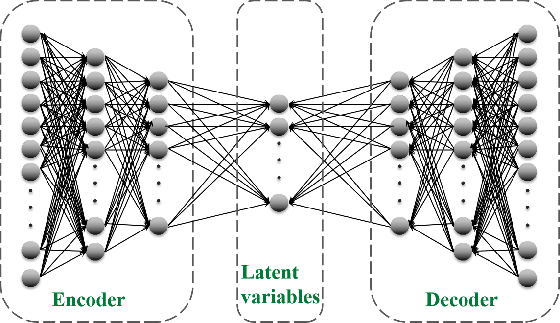
We note that nearly all the improvements on VAE are strongly related to latent variables. Latent variables show the importance even in some industrial applications. We propose the weak convergence approximation algorithms which use part of important latent variables to improve the generative ability of VAE and its variants. The principle of the algorithms is that they equivalently increase the weight of distributions of part of latent variables. Hence we need feature selection algorithms to select latent variables.

Feature selection is widely used during data processing. Feature selection algorithms score every feature and pick the features according to the scores from the largest to the smallest[13]. The aim of them is to pick features which contain useful information and help model avoid overfitting and dimension explosion problems[14]. Naturally, it is not a novel project in the field of machine learning, and some classical methods, such as Laplacian score[15], relevant feature selection[16] etc., have been widely used in data processing. Here, we continue to use this strategy to select latent variables of VAE. Moreover, we propose evidence lower bound difference (ELBD) score to do the selection on latent variables. ELBD uses absolute value of difference of two evidence lower bounds (ELBOs) to score each latent variable. Based on ELBD, generalized ELBD (gELBD) is proposed, and we find that gELBD performs well on classification tasks. We compare ELBD and gELBD with other feature selection algorithms including state-of-the-art algorithms in experiments.

The rest of the paper is organized as follows. Section 2 presents some preliminaries about VAE and its variants, for which two kinds of latent variables are used and the algorithms of training process are proposed, respectively. In Section 3, we state our motivation and purpose. Then we propose the weak convergence approximation algorithms on different types of latent variables, and give theoretical analyses about them. In Section 4, we propose our own feature selection algorithm and generalize it. This is followed by some experimental studies of proposed algorithms in Section 5. Finally, Section 6 concludes the paper.

Notation: Throughout the paper, the bold lowercase letters and Greeks represent row vectors, bold capital letters and Greeks represent matrices, and $(\mathbf{z})_{i}$ or $z_{i}$ represents the $i$th element of row vector $\mathbf{z}$. We also define the norm on vector $\|\mathbf{z}\|=\underset{i}{\max}|z_{i}|$. In addition, only pictures data sets are considered.

2 Preliminaries

In this section, we will introduce shortly VAE and its variants[2], then give the algorithms of training processes for VAE with two kinds of different latent variables.

2.1 VAE

VAE is a kind of typical latent variable model, whose main purpose is to generate sample points sharing the same distribution with the original samples as far as possible through utilizing latent variables.

Let $\mathbb{D}=\{\mathbf{x}_{1},...,\mathbf{x}_{N}\}$ represents a data set, and the task is to infer the distribution of $\mathbf{x}$, $P(\mathbf{x})$, so as to generate new sample points. VAE addresses this issue by introducing latent variables $\mathbf{z}\in\mathbb{R}^{m}$ obeying the standardized normal distribution $\mathcal{N}(\mathbf{0},\mathbf{I})$, and further minimizing the $\mathcal{KL}$ divergence between the true posterior distribution $P(\mathbf{z}|\mathbf{x})$ and the learned one $Q(\mathbf{z}|\mathbf{x})$ on $\mathbb{D}$. Here, the $\mathcal{KL}$ divergence is essential about the expectation calculation, defined by

$$\mathcal{KL}[Q(\mathbf{z}|\mathbf{x})\parallel P(\mathbf{z}|\mathbf{x})]=E_{Q(\mathbf{z}|\mathbf{x})}\left(\log Q(\mathbf{z}|\mathbf{x})-\log P(\mathbf{z}|\mathbf{x})\right).$$ (1)

By adding $P(\mathbf{x})$ and applying Bayes rule to $P(\mathbf{z}|\mathbf{x})$, the above expression can be rewritten as

$$\displaystyle\log P(\mathbf{x})-\mathcal{KL}[Q(\mathbf{z}|\mathbf{x})\parallel P(\mathbf{z}|\mathbf{x})]$$

$$= E_{Q(\mathbf{z}|\mathbf{x})}\left(\log P(\mathbf{x}|\mathbf{z})\right)-\mathcal{KL}[Q(\mathbf{z}|\mathbf{x})\parallel P(\mathbf{z})],$$ (2)

which is the core formula in VAE. The left hand side of the formula is just right the maximization objective with the first term to represent the log-likelihood of $P(\mathbf{x})$ while the second term to express minus error of estimating $P(\mathbf{z}|\mathbf{x})$ by $Q(\mathbf{z}|\mathbf{x})$. The right hand side takes a form of autoencoder. The whole forward process contains following steps: $Q(\mathbf{z}|\mathbf{x})$ which is called encoder, “encodings” original data $\mathbf{x}$ into $\mathbf{z}$, and the “reparameterization trick” is adopted on $\mathbf{z}$. Then $P(\mathbf{x}|\mathbf{z})$ which is called decoder, “decodings” it to reconstruct $\mathbf{x}$. The right side of equation (2) can be also seen as a lower bound of $\log P(\mathbf{x})$ due to the nonnegativity of $\mathcal{KL}[Q(\mathbf{z}|\mathbf{x})\parallel P(\mathbf{z}|\mathbf{x})]$, usually called evidence lower bound (ELBO). The inner two terms are both computable, so the negative ELBO often acts as the cost function one can be optimized via stochastic gradient descent.

To optimize equation (2), it needs to know a specific form about $Q(\mathbf{z}|\mathbf{x})$. The usual choice for it, and also for $P(\mathbf{x}|\mathbf{z})$ and $P(\mathbf{z})$ is the Gaussian distribution, i.e.,

$$Q(\mathbf{z}|\mathbf{x})=\mathcal{N}(\boldsymbol{\mu}(\mathbf{x}),\boldsymbol{\Sigma}(\mathbf{x})),~{}P(\mathbf{x}|\mathbf{z})=\mathcal{N}(\mathbf{f}(\mathbf{z}),\mathbf{I}),~{}p(\mathbf{z})=\mathcal{N}(0,\mathbf{I}),$$ (3)

where $\boldsymbol{\mu}$, $\boldsymbol{\Sigma}$ and $\mathbf{f}$ are arbitrary deterministic functions that can be learned via neural networks. $\mathbf{I}$ is identity matrix. With these distributions, the back propagation can compute a gradient used for stochastic gradient descent, which completes the learning process.

CVAE is a kind of conditional VAE that conditions on the labels of data $\mathbf{y}$ during the entire generative process. Encoder and decoder become $Q(\mathbf{z}|\mathbf{x},\mathbf{y})$ and $P(\mathbf{z}|\mathbf{x},\mathbf{y})$. So it is more potential in handling images that have different categories.

Norm flow VAE (NF-VAE)[17] uses autoregressive function $\mathbf{z}_{t}=\mathbf{z}_{t-1}+\mathbf{p}h(\mathbf{c}^{\top}\mathbf{z}_{t-1}+b)$ to improve the flexible of posterior distribution of latent variables where $h$ is a invertible function and the common choice of $h$ is $\tanh$. NF-VAE is also the stronger version of $\delta$-VAE which treats $h$ as linear function. After going through $T$ norm flowing layers, the latent variables’ distribution can be computed by the equation

$$\log Q(\mathbf{z}_{T}|\mathbf{x})=\log Q(\mathbf{z}_{0}|\mathbf{x})-\sum^{T}_{t=1}\log\det\bigg{|}\frac{d\mathbf{z}_{t}}{d\mathbf{z}_{t-1}}\bigg{|}.$$

Inverse autoregressive flow VAE (IAF-VAE) is a modification of NF-VAE and it is also one of the state-of-the-art generative models. Instead of using $h$, it uses the network to form the autoregressive layers.

$$~{}\left\{\begin{array}[]{lll}\mathbf{m},\mathbf{s}=AutoregressiveNetwork(\mathbf{z}_{t-1},\mathbf{h}),\\ \mathbf{c}=sigmoid(\mathbf{s}),\\ \mathbf{z}_{t}=\mathbf{c}\otimes\mathbf{z}_{t-1}+(\mathbf{1}-\mathbf{c})\otimes\mathbf{m}.\end{array}\right.$$

where the symbol $\otimes$ represents the element-wise multiplication and $\mathbf{h}$ is one of the output of encoder.

The aims of NF-VAE and IAF-VAE are that they expand the range of latent variables’ distribution, make them not only be constrained in the family of Gaussian distribution. However, we can also see them as a part of decoder function in the forward process and we only consider $\mathbf{z}_{0}$ in NF-VAE and IAF-VAE whose posterior distribution is still Gaussian distribution in equation (3).

In this and latter sections, we only show algorithms on original VAE, the corresponding algorithms on CVAE, NF-VAE, IAF-VAE or any other variant models of VAE can be expanded naturally. And in Section 5, we take experiments on VAE, CVAE, NF-VAE and IAF-VAE.

2.2 Mean-field and full-covariance Gaussian posterior

This subsection introduces two types of Gaussian posterior of latent variables: mean-field and full-covariance[18]. The mean-field Gaussian posterior assumes the $\boldsymbol{\Sigma}(\mathbf{x})$ in $Q(\mathbf{z}|\mathbf{x})$ as the diagonal matrix. Oppositely, the full-covariance Gaussian posterior makes $\boldsymbol{\Sigma}(\mathbf{x})$ be a full matrix to train. We take original VAE as an example, and the training processes are shown in Algorithm 1 and Algorithm 2.

Algorithm 1 The training process of VAE with mean-field Gaussian posterior

0:  data set $\mathbb{D}=\{\mathbf{x}_{1},...,\mathbf{x}_{N}\}$

1:  for  data $\mathbf{x}$ in $\mathbb{D}$ do

2:     $\boldsymbol{\mu}$, $\log\boldsymbol{\sigma}^{2}=EncoderNetwork(\mathbf{x})$;

3:     sample $\boldsymbol{\epsilon}$ from normal distribution $\mathcal{N}(0,\mathbf{I})$;

4:     $\mathbf{z}=\boldsymbol{\epsilon}\otimes\exp(\frac{1}{2}\log\boldsymbol{\sigma}^{2})+\boldsymbol{\mu}$;

5:     $\mathbf{x}^{\prime}=DecoderNetwork(\mathbf{z})$;

6:     $loss=\frac{1}{2}\overset{\dim\mathbf{x}}{\underset{i=1}{\sum}}(\mathbf{x}^{\prime}-\mathbf{x})_{i}^{2}+\frac{1}{2}\overset{\dim\mathbf{z}}{\underset{i=1}{\sum}}(\boldsymbol{\mu}^{2}+\exp(\log\boldsymbol{\sigma}^{2})-\log\boldsymbol{\sigma}^{2}-1)_{i}$;

7:     optimize the $loss$ by gradient descent methods;

8:  end for

We put original data $\mathbf{x}$ in the encoder network and obtain the $\boldsymbol{\mu}$ and $\log\boldsymbol{\sigma}^{2}$ where $\boldsymbol{\mu}$ is the mean of $Q(\mathbf{z}|\mathbf{x})$, $\boldsymbol{\sigma}^{2}$ is the diagonal of the covariance matrix $\boldsymbol{\Sigma}(\mathbf{x})$ in equation (3). Line 3 and Line 4 are called reparameterization. It generates latent variables $\mathbf{z}$ and makes sure $\mathbf{z}$ follow $\mathcal{N}\left(\boldsymbol{\mu}(\mathbf{x}),\boldsymbol{\Sigma}(\mathbf{x})\right)$. Then we feed $\mathbf{z}$ in the decoder network to get a new data $\mathbf{x}^{\prime}$ in line 5. The loss function in line 6 is negative ELBO after putting the equation (3) into equation (2) where $\dim\mathbf{x}$ and $\dim\mathbf{z}$ are the dimension of row vectors $\mathbf{x}$ and $\mathbf{z}$. And it is also the loss we need to optimize in line 7.

Algorithm 2 The training process of VAE with full-covariance Gaussian posterior

0:  data set $\mathbb{D}=\{\mathbf{x}_{1},...,\mathbf{x}_{N}\}$

1:  for  data $\mathbf{x}$ in $\mathbb{D}$ do

2:     $\boldsymbol{\mu}$, $\log\boldsymbol{\sigma}$, $\mathbf{L}_{m}=EncoderNetwork(\mathbf{x})$;

3:     mask matrix $\mathbf{L}_{m}$ and turn the $\mathbf{L}_{m}$ to lower triangular matrix with zeros on and above the diagonal;

4:     $\mathbf{L}=\mathbf{L}_{m}+diag(\exp(\boldsymbol{\sigma}))$;

5:     sample $\boldsymbol{\epsilon}$ from normal distribution $\mathcal{N}(0,\mathbf{I})$;

6:     $\mathbf{z}=\boldsymbol{\mu}+\boldsymbol{\epsilon}\mathbf{L}$;

7:     $\mathbf{x}^{\prime}=DecoderNetwork(\mathbf{z})$;

8:     $L_{1}=-\frac{1}{2}\overset{\dim\mathbf{z}}{\underset{i=1}{\sum}}(\boldsymbol{\epsilon}^{2}+\log(2\pi)+\log\boldsymbol{\sigma})_{i}$;

9:     $L_{2}=-\frac{1}{2}\overset{\dim\mathbf{z}}{\underset{i=1}{\sum}}(\mathbf{z}^{2}+\log(2\pi))_{i}$;

10:     $L_{3}=\frac{1}{2}\overset{\dim\mathbf{x}}{\underset{i=1}{\sum}}(\mathbf{x}^{\prime}-\mathbf{x})_{i}^{2}$

11:     $loss=L_{3}+L_{1}-L_{2}$;

12:     optimize the $loss$ by gradient descent methods;

13:  end for

Instead of outputting $\log\boldsymbol{\sigma}^{2}$, encoder network outputs $\log\boldsymbol{\sigma}$ and $\mathbf{L}_{m}$ in full-covariance condition. We still take $\boldsymbol{\sigma}^{2}$ as the diagon of $\boldsymbol{\Sigma}(\mathbf{x})$. After the mask operation in line 3, we see the $\mathbf{L}$ in line 4 as the Cholesky factorization of symmetric positive definite matrix $\boldsymbol{\Sigma}(\mathbf{x})$[19]. Then latent variables $\mathbf{z}$ follow $\mathcal{N}\left(\boldsymbol{\mu},\mathbf{L}\mathbf{L}^{\top}\right)$ after reparameterization. It should be noted that in line 11, $L_{1}-L_{2}$ is not the exact $\mathcal{KL}$ divergence but the unbiased estimation of it, i.e., $E_{Q(\mathbf{z}|\mathbf{x})}(L_{1}-L_{2})=\mathcal{KL}[Q(\mathbf{z}|\mathbf{x})\parallel P(\mathbf{z})]$.

3 Optimize VAE using selected features

In this section, we state how we use the features we pick to increase the ELBO and why we do the features selection on latent variables.

3.1 Marginalization of encoder

For the sake of simplicity and clarity, we separate the latent variables $\mathbf{z}$ as two sets $\mathbf{w}$ and $\mathbf{u}$, i.e., $\mathbf{z}=(\mathbf{w},\mathbf{u})$ where $\mathbf{u}$ are the features we select by some feature selection algorithms. We eliminate the variables $\mathbf{u}$ in the distributions $Q(\mathbf{w},\mathbf{u}|\mathbf{x})$ and $P(\mathbf{w},\mathbf{u}|\mathbf{x})$. According to the equation (1), the loss after elimination is $\mathcal{KL}[Q(\mathbf{w}|\mathbf{x})\parallel P(\mathbf{w}|\mathbf{x})]$ where $Q(\mathbf{w}|\mathbf{x})=\int^{+\infty}_{-\infty}Q(\mathbf{w},\mathbf{u}|\mathbf{x})d\mathbf{u}$, $P(\mathbf{w}|\mathbf{x})=\int^{+\infty}_{-\infty}P(\mathbf{w},\mathbf{u}|\mathbf{x})d\mathbf{u}$.

Subtracting the two losses and using the equation (1), we get

$$\mathcal{KL}[Q(\mathbf{w},\mathbf{u}|\mathbf{x})\parallel P(\mathbf{w},\mathbf{u}|\mathbf{x})]-\mathcal{KL}[Q(\mathbf{w}|\mathbf{x})\parallel P(\mathbf{w}|\mathbf{x})]$$

$$= E_{Q(\mathbf{w}|\mathbf{x})}\left(\mathcal{KL}[Q(\mathbf{u}|\mathbf{w},\mathbf{x})\parallel P(\mathbf{u}|\mathbf{w},\mathbf{x})]\right)\geq 0.$$

The equation above demonstrates that the distributions after elimination can decrease the $\mathcal{KL}$ divergence in equation (1) so that increase the ELBO. According to the inference from equation (1) to equation (2), we have

Proposition 1.

Let $\mathbf{z}$ be the latent variables of VAE model and $\mathbf{z}=(\mathbf{w},\mathbf{u})$, then

$$E_{Q(\mathbf{z}|\mathbf{x})}\left(\log P(\mathbf{x}|\mathbf{z})\right)-\mathcal{KL}[Q(\mathbf{z}|\mathbf{x})\parallel P(\mathbf{z})]$$

$$\leq E_{Q(\mathbf{w}|\mathbf{x})}\left(\log P(\mathbf{x}|\mathbf{w})\right)-\mathcal{KL}[Q(\mathbf{w}|\mathbf{x})\parallel P(\mathbf{w})],$$

where

$$P(\mathbf{x}|\mathbf{w})=\int^{+\infty}_{-\infty}P(\mathbf{x}|\mathbf{z})Q(\mathbf{u}|\mathbf{w},\mathbf{x})d\mathbf{u},~{}Q(\mathbf{w}|\mathbf{x})=\int^{+\infty}_{-\infty}Q(\mathbf{z}|\mathbf{x})d\mathbf{u}.$$ (5)

Proof.

The detailed proof can be found in Appendix. ∎

Thus our goal of this section is to use the VAE model which is already trained to approximate the model with only $\mathbf{w}$ as latent variables, so that we can achieve a higher ELBO:

$$E_{Q(\mathbf{w}|\mathbf{x})}\left(\log P(\mathbf{x}|\mathbf{w})\right)-\mathcal{KL}[Q(\mathbf{w}|\mathbf{x})\parallel P(\mathbf{w})].$$ (6)

Proposition 1 points out a method to obtain the encoder and decoder in the equation (6).

Fortunately, the integral operation on Gaussian distribution $Q(\mathbf{z}|\mathbf{x})$ is simply computing the marginal distribution of $\mathbf{w}$. Let us assume

$$Q(\mathbf{z}|\mathbf{x})=Q(\mathbf{w},\mathbf{u}|\mathbf{x})=\mathcal{N}\left(\left(\boldsymbol{\mu}_{\mathbf{w}}(\mathbf{x}),\boldsymbol{\mu}_{\mathbf{u}}(\mathbf{x})\right),\ \begin{pmatrix}\boldsymbol{\Sigma}_{\mathbf{w}\mathbf{w}}(\mathbf{x})&\boldsymbol{\Sigma}_{\mathbf{w}\mathbf{u}}(\mathbf{x})\\ \boldsymbol{\Sigma}_{\mathbf{u}\mathbf{w}}(\mathbf{x})&\boldsymbol{\Sigma}_{\mathbf{u}\mathbf{u}}(\mathbf{x})\end{pmatrix}\right).$$

Then the marginal distribution is

$$Q(\mathbf{w}|\mathbf{x})=\mathcal{N}\left(\boldsymbol{\mu}_{\mathbf{w}}(\mathbf{x}),\boldsymbol{\Sigma}_{\mathbf{w}\mathbf{w}}(\mathbf{x})\right).$$

To achieve this marginalization, we introduce a special $\dim\mathbf{z}$-dimensional vector $\boldsymbol{\pi}$, whose elements are ones or zeros, to build a new model with latent variables $\mathbf{z}\otimes\boldsymbol{\pi}$. We assume $\boldsymbol{\pi}=(\underset{\dim\mathbf{w}}{\underbrace{1,...,1}},\underset{\dim\mathbf{u}}{\underbrace{0,...,0}})$, and then define

$$Q(\mathbf{z}\otimes\boldsymbol{\pi}|\mathbf{x})=\mathcal{N}\left(\left(\boldsymbol{\mu}_{\mathbf{w}}(\mathbf{x}),\mathbf{0}_{1\times\dim\mathbf{u}}\right),\ \begin{pmatrix}\boldsymbol{\Sigma}_{\mathbf{w}\mathbf{w}}(\mathbf{x})&\mathbf{0}_{\dim\mathbf{w}\times\dim\mathbf{u}}\\ \mathbf{0}_{\dim\mathbf{u}\times\dim\mathbf{w}}&\mathbf{I}_{\dim\mathbf{u}\times\dim\mathbf{u}}\end{pmatrix}\right),$$

where $\mathbf{0}_{d_{1}\times d_{2}}$ is $d_{1}\times d_{2}$ matrix whose elements are all zeros, and $\mathbf{I}_{d\times d}$ is $d\times d$ identity matrix.

Our aim is to derive the $\mathcal{KL}$ divergence after marginalization of encoder. So we put $Q(\mathbf{z}\otimes\boldsymbol{\pi}|\mathbf{x})$ in the $\mathcal{KL}$ divergence in equation (2), then

$$\mathcal{KL}[Q(\mathbf{z}\otimes\boldsymbol{\pi}|\mathbf{x})\parallel P(\mathbf{z})] =\mathcal{KL}[Q(\mathbf{w}|\mathbf{x})P(\mathbf{u})\parallel P(\mathbf{w})P(\mathbf{u})]$$

$$=\mathcal{KL}[Q(\mathbf{w}|\mathbf{x})\parallel P(\mathbf{w})],$$

which completes the marginalization of encoder in Proposition 1. The algorithms that achieve the marginalization of $Q(\mathbf{z}|\mathbf{x})$ with mean-field and full-covariance Gaussian posterior are shown in Algorithm 3 and Algorithm 4

Algorithm 3 The marginalization of encoder with mean-field Gaussian posterior

0:  data set $\mathbb{D}=\{\mathbf{x}_{1},...,\mathbf{x}_{N}\}$, VAE model, $\boldsymbol{\pi}$

1:  for  data $\mathbf{x}$ in $\mathbb{D}$ do

2:     $\boldsymbol{\mu}$, $\log\boldsymbol{\sigma}^{2}=EncoderNetwork(\mathbf{x})$;

3:     $\boldsymbol{\mu}=\boldsymbol{\mu}\otimes\boldsymbol{\pi}$, $\log\boldsymbol{\sigma}^{2}=\log\boldsymbol{\sigma}^{2}\otimes\boldsymbol{\pi}$;

4:     $\mathcal{KL}=\mathcal{KL}+\frac{1}{2}\overset{\dim\mathbf{z}}{\underset{i=1}{\sum}}(\boldsymbol{\mu}^{2}+\exp(\log\boldsymbol{\sigma}^{2})-\log\boldsymbol{\sigma}^{2}-1)_{i}$;

5:  end for

6:  $\mathcal{KL}=\mathcal{KL}/N$;

6:  $\mathcal{KL}$

Algorithm 4 The marginalization of encoder with full-covariance Gaussian posterior

0:  data set $\mathbb{D}=\{\mathbf{x}_{1},...,\mathbf{x}_{N}\}$, VAE model, $\boldsymbol{\pi}$

1:  for  data $\mathbf{x}$ in $\mathbb{D}$ do

2:     $\boldsymbol{\mu}$, $\log\boldsymbol{\sigma}$, $\mathbf{L}_{m}=EncoderNetwork(\mathbf{x})$;

3:     mask matrix $\mathbf{L}_{m}$ and turn the $\mathbf{L}_{m}$ to lower triangular matrix with zeros on and above the diagonal;

4:     $\boldsymbol{\mu}=\boldsymbol{\mu}\otimes\boldsymbol{\pi}$, $\log\boldsymbol{\sigma}=\log\boldsymbol{\sigma}\otimes\boldsymbol{\pi}$, $\mathbf{L}_{m}=\boldsymbol{\pi}\otimes\mathbf{L}_{m}\otimes\boldsymbol{\pi}^{\top}$;

5:     $\mathbf{L}=\mathbf{L}_{m}+diag(\exp(\boldsymbol{\sigma}))$;

6:     sample $\boldsymbol{\epsilon}$ from normal distribution $\mathcal{N}(0,\mathbf{I})$;

7:     $\mathbf{w}=\boldsymbol{\mu}+\boldsymbol{\epsilon}\mathbf{L}$;

8:     $L_{1}=-\frac{1}{2}\overset{\dim\mathbf{z}}{\underset{i=1}{\sum}}(\boldsymbol{\epsilon}^{2}+\log(2\pi)+\log\boldsymbol{\sigma})_{i}$;

9:     $L_{2}=-\frac{1}{2}\overset{\dim\mathbf{z}}{\underset{i=1}{\sum}}(\mathbf{w}^{2}+\log(2\pi))_{i}$;

10:     $\mathcal{KL}=\mathcal{KL}+(L_{1}-L_{2})$;

11:  end for

12:  $\mathcal{KL}=\mathcal{KL}/N$;

12:  $\mathcal{KL}$

The input VAE model is already trained and $\boldsymbol{\pi}$ in these algorithms is generated by the feature selection algorithms. The indices of zero elements in $\boldsymbol{\pi}$ are also the indices of elements of $\mathbf{u}$ among $\mathbf{z}$. These two algorithms output values of $\mathcal{KL}$ divergence after marginalization of encoder. The differences of Algorithm 3 and Algorithm 4 from Algorithm 1 and Algorithm 2 are mean and variance which element-wise multiply by $\boldsymbol{\pi}$. In line 4 of Algorithm 4, $\boldsymbol{\pi}\otimes\mathbf{L}_{m}$ ($\mathbf{L}_{m}\otimes\boldsymbol{\pi}^{\top}$) represents each row (column) vector of matrix $\mathbf{L}_{m}$ element-wise multiply by $\boldsymbol{\pi}$ ($\boldsymbol{\pi}^{\top}$). These procedures guarantee $\mathbf{u}$ follow standard normal distribution and are independent with $\mathbf{w}$.

It should be noted that Algorithm 3 and Algorithm 4 seem to have little contribution on generating pictures. They are more likely giving a mathematical explanation that the ELBO we compute after optimization is the approximation of equation (6).

3.2 Weak convergence approximation of decoder

The integral of decoder $P(\mathbf{x}|\mathbf{z})$ in equation (5) is much more complicated. Exact distribution after integral operations in equation (5) is almost impossible. Therefore we need to use other ways to approximate it. Integral of decoder in equation (5) can be transformed into expectation, i.e.,

$$P(\mathbf{x}|\mathbf{w})=\int^{+\infty}_{-\infty}P(\mathbf{x}|\mathbf{z})Q(\mathbf{u}|\mathbf{w},\mathbf{x})d\mathbf{u}=E_{Q(\mathbf{u}|\mathbf{w},\mathbf{x})}\left(P(\mathbf{x}|\mathbf{z})\right).$$

Let $\frac{1}{K}\overset{K}{\underset{j=1}{\sum}}P(\mathbf{x}|\mathbf{w},\mathbf{u}_{j})$ be function of random variables $\mathbf{u}_{j}$ for any given $\mathbf{w}$ and $\mathbf{x}$ where $\mathbf{u}_{j}$ is sampled i.i.d from $Q(\mathbf{u}|\mathbf{w},\mathbf{x})$. By the strong law of large numbers, $\frac{1}{K}\overset{K}{\underset{j=1}{\sum}}P(\mathbf{x}|\mathbf{w},\mathbf{u}_{j})$ converges to $E_{Q(\mathbf{u}|\mathbf{w},\mathbf{x})}\left(P(\mathbf{x}|\mathbf{z})\right)$ almost everywhere[20], i.e.,

$$P\left(\lim_{K\to\infty}\frac{1}{K}\sum^{K}_{j=1}P(\mathbf{x}|\mathbf{w},\mathbf{u}_{j})=E_{Q(\mathbf{u}|\mathbf{w},\mathbf{x})}\left(P(\mathbf{x}|\mathbf{z})\right)\right)=1.$$

Since $\mathbf{u}_{j}$ are sampled from $Q(\mathbf{u}|\mathbf{w},\mathbf{x})$ and not influenced by generated data $\mathbf{x}$ in decoder, then for given $\mathbf{w}$, we can sample a infinite sequence $\{\mathbf{u}_{1},\mathbf{u}_{2},...\}$ in probability 1, such that $\frac{1}{K}\overset{K}{\underset{j=1}{\sum}}P(\mathbf{x}|\mathbf{w},\mathbf{u}_{j})$ converges to $E_{Q(\mathbf{u}|\mathbf{w},\mathbf{x})}\left(P(\mathbf{x}|\mathbf{z})\right)=P(\mathbf{x}|\mathbf{w})$. Then by the measure theory[20], we can definitely find a sequence $\{\mathbf{u}_{1},\mathbf{u}_{2},...\}$ for every $\mathbf{w}$ to achieve the convergence. We fix these uncountable sequences and assume projections $\{\mathbf{u}_{1}(\mathbf{w}),\mathbf{u}_{2}(\mathbf{w}),...\}$ project every $\mathbf{w}$ to these sequences. However if $\mathbf{w}$ and $\mathbf{u}$ are independent, these projections will become constants. Then $\frac{1}{K}\overset{K}{\underset{j=1}{\sum}}P(\mathbf{x}|\mathbf{w},\mathbf{u}_{j}(\mathbf{w}))$ converges to $E_{Q(\mathbf{u}|\mathbf{w},\mathbf{x})}\left(P(\mathbf{x}|\mathbf{z})\right)=P(\mathbf{x}|\mathbf{w})$ point-by-point. We write $\mathbf{u}_{j}(\mathbf{w})$ as $\mathbf{u}_{j}$ for short in latter easy and let $M_{K}(\mathbf{x}|\mathbf{w})=\frac{1}{K}\overset{K}{\underset{j=1}{\sum}}P(\mathbf{x}|\mathbf{w},\mathbf{u}_{j})$ as conditional distribution of $\mathbf{x}$ given $\mathbf{w}$.

$M_{K}(\mathbf{x}|\mathbf{w})$ as a Gaussian mixture distribution will lead to a lot of computation problems if we use it directly as the approximation to $P(\mathbf{x}|\mathbf{w})$ in ELBO. Considering $P(\mathbf{x}|\mathbf{w})$ is a Gaussian distribution, we want to project $M_{K}(\mathbf{x}|\mathbf{w})$ into the family of Gaussian distributions and use the projection as the approximation. The approximation in the same family of distributions should be much more efficient and less complex. The following theorem proposes a way of projection using $\mathcal{KL}$ divergence.

Theorem 1.

Let $M_{K}(\mathbf{x}|\mathbf{w})=\frac{1}{K}\overset{K}{\underset{j}{\sum}}P(\mathbf{x}|\mathbf{w},\mathbf{u}_{j})=\frac{1}{K}\overset{K}{\underset{j}{\sum}}\mathcal{N}\left(\mathbf{x}|\mathbf{f}(\mathbf{w},\mathbf{u}_{j}),\mathbf{I}\right)$ and $P_{K}(\mathbf{x}|\mathbf{w})=\mathcal{N}(\boldsymbol{\mu}_{K}(\mathbf{w}),\mathbf{I})$. Then

$$\underset{\boldsymbol{\mu}_{K}}{\arg\min}\mathcal{KL}[M_{K}(\mathbf{x}|\mathbf{w})\parallel P_{K}(\mathbf{x}|\mathbf{w})]=\frac{1}{K}\sum^{K}_{j=1}\mathbf{f}(\mathbf{w},\mathbf{u}_{j}).$$

We call this M-projection.

Proof.

The detailed proof can be found in Appendix. ∎

Note that we use VAE to generate pictures, the value of every pixel is in interval $[0,1]$. Thus we usually constrain the mean of decoder $\mathbf{f}(\mathbf{z})$ by activation function $\tanh$ or $sigmoid$ function, which means for every element in $\mathbf{f}(\mathbf{z})$, $0\leq\big{|}f_{i}(\mathbf{z})\big{|}\leq 1$ for any $\mathbf{z}$. Using this assumption, we give an important lemma to explore the connection between $P(\mathbf{x}|\mathbf{w})$ and $P_{K}(\mathbf{x}|\mathbf{w})$.

Lemma 1.

Let $P(\mathbf{x}|\mathbf{w},\mathbf{u})=\mathcal{N}(\mathbf{f}(\mathbf{w},\mathbf{u}),\mathbf{I})$. If $\mathbf{f}$ is bounded, i.e., there is a constant $C$ s.t. $\|\mathbf{f}(\mathbf{w},\mathbf{u})\|\leq C$ for all $\mathbf{w}$ and $\mathbf{u}$. Then for any non-negative integrable function $g(y,\mathbf{x})$ with respect to $\mathbf{x}$ on $(-\infty,+\infty)$, and $g(y,\mathbf{x})$ is monotone with respect to $y$, integral operation and limit operation are exchangeable, i.e.,

$$\lim_{K\to\infty}\int^{+\infty}_{-\infty}g(M_{K}(\mathbf{x}|\mathbf{w}),\mathbf{x})d\mathbf{x}=\int^{+\infty}_{-\infty}\lim_{K\to\infty}g(M_{K}(\mathbf{x}|\mathbf{w}),\mathbf{x})d\mathbf{x}.$$

Proof.

The detailed proof can be found in Appendix. ∎

Figure 2: The black lines are three examples of $P(\mathbf{x}|\mathbf{w},\mathbf{u}_{j})$. These three examples are Gaussian distributions with different means. Since mean function $\mathbf{f}(\mathbf{w},\mathbf{u}_{j})$ is bounded $\|\mathbf{f}(\mathbf{w},\mathbf{u}_{j})\|\leq 1$ and maximal values are all the same, we can use function $G$, the red dotted line which is also integrable on $(-\infty,+\infty)$, to dominate all $P(\mathbf{x}|\mathbf{w},\mathbf{u}_{j})$, then to dominate all $M_{K}(\mathbf{x}|\mathbf{w})$. Then the Lemma 1 is directed result of the dominated convergence theorem[21].

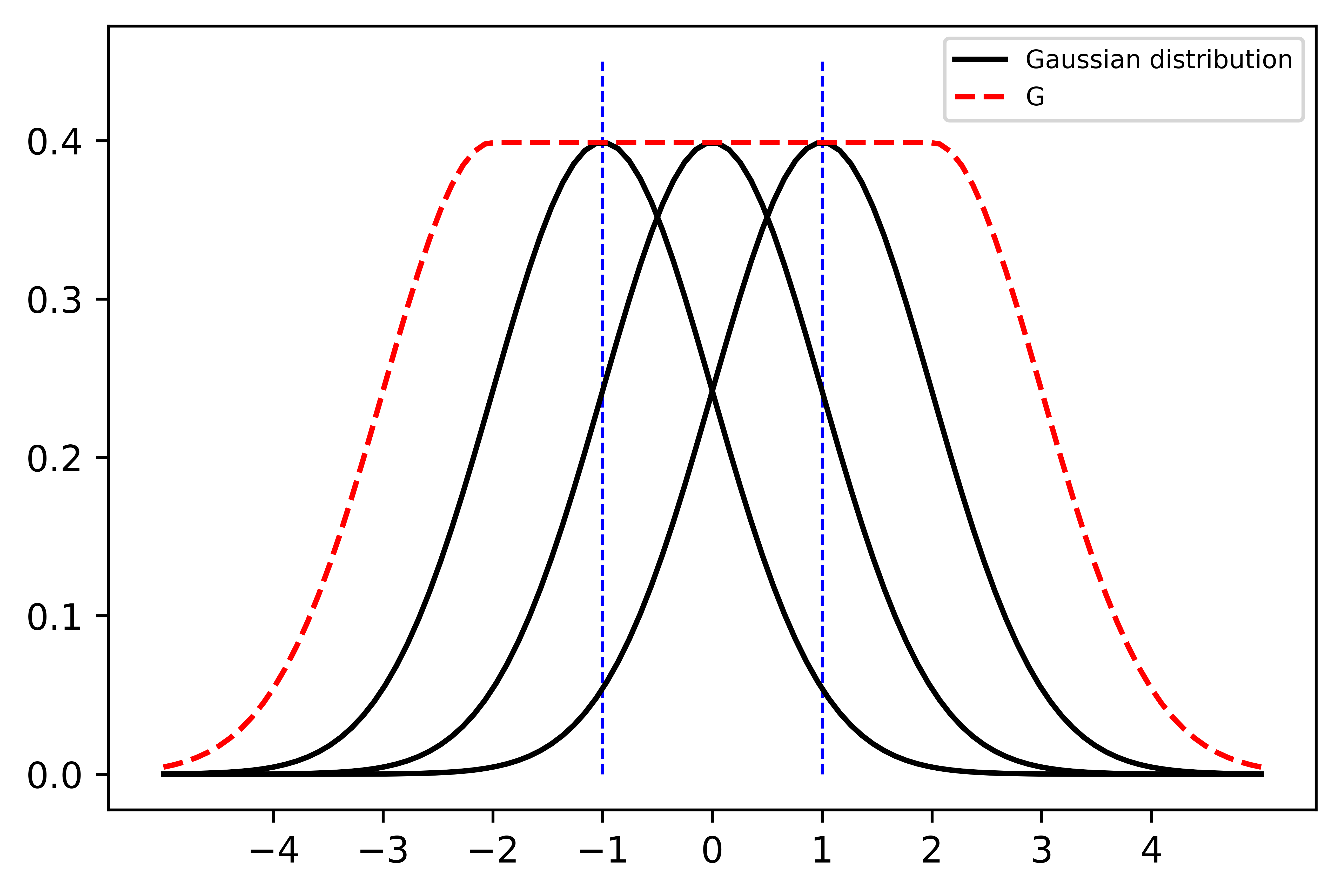
The Figure 2 states the reason why we must need to constrain the $\mathbf{f}(\mathbf{z})$. We may use this assumption that $\mathbf{f}$ is bounded in this and latter section without mentioning it. We only know $M_{K}(\mathbf{x}|\mathbf{w})$ converges to $P(\mathbf{x}|\mathbf{w})$ point-by-point, but we still need to do integral operation on $M_{K}(\mathbf{x}|\mathbf{w})$. Lemma 1 guarantees the exchange of limit and integral. Now we can compute the mean and variance of $P(\mathbf{x}|\mathbf{w})$.

Theorem 2.

Let random variables $\boldsymbol{\xi}\sim P(\mathbf{x}|\mathbf{w})$ and $\boldsymbol{\xi}_{K}\sim M_{K}(\mathbf{x}|\mathbf{w})$. Let $P_{K}(\mathbf{x}|\mathbf{w})=\mathcal{N}(\mathbf{x}|\boldsymbol{\mu}_{K}(\mathbf{w}),\mathbf{I})=\mathcal{N}\left(\mathbf{x}\bigg{|}\frac{1}{K}\overset{K}{\underset{j=1}{\sum}}\mathbf{f}(\mathbf{w},\mathbf{u}_{j}),\mathbf{I}\right)$, then

$$E(\boldsymbol{\xi})=\lim_{K\to\infty}E(\boldsymbol{\xi}_{K})=\lim_{K\to\infty}\boldsymbol{\mu}_{K},\ \ \ \ D(\boldsymbol{\xi})=\lim_{K\to\infty}D(\boldsymbol{\xi}_{K})=\mathbf{I}.$$

Proof.

The detailed proof can be found in Appendix. ∎

By the Theorem 2, it is trivial to have that the distribution $P_{K}(\mathbf{x}|\mathbf{w})$ converges to $P(\mathbf{x}|\mathbf{w})$. But it should be noted that the convergence of mean and covariance matrix is independent with $\mathbf{x}$, then we can unconditionally exchange limit operation with respect to $K$ and integral on $h(P_{K}(\mathbf{x}|\mathbf{w}))$ related to $\mathbf{x}$ for any function $h$. According to the discussion, we have the theorem below.

Theorem 3.

Let random variables $\boldsymbol{\eta}_{K}\sim\mathcal{N}\left(\mathbf{x}\bigg{|}\frac{1}{K}\overset{K}{\underset{j=1}{\sum}}\mathbf{f}(\mathbf{w},\mathbf{u}_{j}),\mathbf{I}\right)=P_{K}(\mathbf{x}|\mathbf{w})$ and $\boldsymbol{\xi}\sim P(\mathbf{x}|\mathbf{w})$, then $\boldsymbol{\eta}_{K}$ converges to $\boldsymbol{\xi}$ in distribution. Moreover,

$$\lim_{K\to\infty}\mathcal{KL}[P_{K}(\mathbf{x}|\mathbf{w})\parallel P(\mathbf{x}|\mathbf{w})]=\lim_{K\to\infty}\mathcal{KL}[P(\mathbf{x}|\mathbf{w})\parallel P_{K}(\mathbf{x}|\mathbf{w})]=0.$$

Proof.

The detailed proof can be found in Appendix. ∎

From the Theorem 3, we have a good method to approximate $P(\mathbf{x}|\mathbf{w})$. Since By the definition of convergence in distribution, $P_{K}(\mathbf{x}|\mathbf{w})$ weak converges to $P(\mathbf{x}|\mathbf{w})$, we call this approximation as weak convergence approximation.

In the mean-field condition, latent variables $\mathbf{u}$ and $\mathbf{w}$ are independent. However in full-covariance condition, the computation of mean and covariance matrix in $Q(\mathbf{u}|\mathbf{w},\mathbf{x})$ is complex. To simplify it, we can pick $\mathbf{u}$ are independent with $\mathbf{w}$ as much as possible in feature selection process. Then $Q(\mathbf{u}|\mathbf{w},\mathbf{x})=Q(\mathbf{u}|\mathbf{x})$ which is marginal distribution of encoder $Q(\mathbf{z}|\mathbf{x})$. We can pick sample of $\mathbf{u}$ from sample of $\mathbf{z}$ correspond to the indices of elements of $\mathbf{u}$ among $\mathbf{z}$. Combing these above, we have the weak convergence approximation algorithms of decoder in Algorithm 5 and Algorithm 6.

Algorithm 5 Weak convergence approximation of decoder with mean-field Gaussian posterior

0:  data $\mathbf{x}$, VAE Model, $\boldsymbol{\pi}$, $K$

1:  $\boldsymbol{\mu}$, $\log\boldsymbol{\sigma}^{2}=EncoderNetwork(\mathbf{x}$);

2:  sample $\boldsymbol{\epsilon}$ from normal distribution $\mathcal{N}(0,\mathbf{I})$

3:  $\mathbf{z}=\boldsymbol{\epsilon}\otimes\exp(\frac{1}{2}\log\boldsymbol{\sigma}^{2})+\boldsymbol{\mu}$;

4:  $j=0$, $\mathbf{x}^{\prime}=0$;

5:  while $j<K$ do

6:     sample $\widetilde{\boldsymbol{\epsilon}}$ from normal distribution $\mathcal{N}(0,\mathbf{I})$;

7:     $\widetilde{\mathbf{z}}=\widetilde{\boldsymbol{\epsilon}}\otimes\exp(0.5\log\boldsymbol{\sigma}^{2})+\boldsymbol{\mu}$;

8:     for every index of selected feature $i$ where $\pi_{i}$=0 do

9:        $z_{i}=\widetilde{z_{i}}$;

10:     end for

11:     $\mathbf{x}^{\prime}=\mathbf{x}^{\prime}+DecoderNetwork(\mathbf{z})/K$;

12:     $j=j+1$;

13:  end while

13:  $\mathbf{x}^{\prime}$

In Algorithm 5, We input the already trained model. After getting latent variables $\mathbf{z}$, we generate $\widetilde{\mathbf{z}}$ in the same way in line 7. By the Theorem 3, we need to sample $\mathbf{u}$ $K$ times from marginal distribution $Q(\mathbf{u}|\mathbf{x})$, so we replace $z_{i}$ with $\widetilde{z}_{i}$ in line 9 where $i$ is a index of element of $\mathbf{u}$ among $\mathbf{z}$, then put the new $\mathbf{z}$ in the decoder network in line 11. The values of $\mathbf{w}$ are fixed after line 5. The $\mathbf{x}^{\prime}$ generated after $K$ epochs is the mean of $P_{K}(\mathbf{x}|\mathbf{w})$, i.e., $\mathbf{x}^{\prime}=\frac{1}{K}\overset{K}{\underset{j=1}{\sum}}\mathbf{f}(\mathbf{w},\mathbf{u}_{j})$. At last, algorithm outputs the $\mathbf{x}^{\prime}$ as the new pictures. The approximation of decoder in full-covariance condition is similar.

Algorithm 6 Weak convergence approximation of decoder with full-covariance Gaussian posterior

0:  data $\mathbf{x}$, VAE Model, $\boldsymbol{\pi}$, $K$

1:  $\boldsymbol{\mu}$, $\log\boldsymbol{\sigma}$, $\mathbf{L}_{m}=EncoderNetwork(\mathbf{x}$);

2:  mask matrix $\mathbf{L}_{m}$ and turn the $\mathbf{L}_{m}$ to upper triangular matrix with zeros on and above the diagonal;

3:  $\mathbf{L}=\mathbf{L}_{m}+diag(\exp(\boldsymbol{\sigma}))$;

4:  sample $\boldsymbol{\epsilon}$ from normal distribution $\mathcal{N}(0,\mathbf{I})$

5:  $\mathbf{z}=\boldsymbol{\mu}+\boldsymbol{\epsilon}\mathbf{L}$;

6:  $j=0$, $\mathbf{x}^{\prime}=0$;

7:  while $j<K$ do

8:     sample $\widetilde{\boldsymbol{\epsilon}}$ from normal distribution $\mathcal{N}(0,\mathbf{I})$;

9:     $\widetilde{\mathbf{z}}=\boldsymbol{\mu}+\widetilde{\boldsymbol{\epsilon}}\mathbf{L}$;

10:     for every index of selected feature $i$ where $\pi_{i}$=0 do

11:        $z_{i}=\widetilde{z_{i}}$;

12:     end for

13:     $\mathbf{x}^{\prime}=\mathbf{x}^{\prime}+DecoderNetwork(\mathbf{z})/K$;

14:     $j=j+1$;

15:  end while

15:  $\mathbf{x}^{\prime}$

In the Algorithm 5 and Algorithm 6, $K$ is the only hyperparameter. We need to analyse the relation between $K$ and ELBO. Firstly, let we consider $K=1$. Assumimg $\mathbf{w}$ and $\mathbf{u}$ are independent, we put $P_{K}(\mathbf{x}|\mathbf{w})$ into first part of ELBO, then we have

$$E_{Q(\mathbf{z}|\mathbf{x})}\left(\log P_{K}(\mathbf{x}|\mathbf{w})\right) =E_{Q(\mathbf{z}|\mathbf{w})}\left(\log P(\mathbf{x}|\mathbf{w},\mathbf{u}_{1})\right)$$

$$=E_{Q(\mathbf{w}|\mathbf{x})}\left(E_{Q(\mathbf{u}|\mathbf{x})}\left(\log P(\mathbf{x}|\mathbf{w},\mathbf{u})\right)\right)$$

$$<E_{Q(\mathbf{w}|\mathbf{u})}\left(\log E_{Q(\mathbf{u}|\mathbf{x})}P(\mathbf{x}|\mathbf{w},\mathbf{u})\right)$$

$$=E_{Q(\mathbf{w}|\mathbf{u})}\left(\log P(\mathbf{x}|\mathbf{w})\right).$$

Therefore, the condition that $K=1$ does not change the decoder. We also can find that $E_{Q(\mathbf{z}|\mathbf{x})}\left(\log P(\mathbf{x}|\mathbf{z})\right)$ is strictly smaller that $E_{Q(\mathbf{w}|\mathbf{x})}\left(\log P(\mathbf{x}|\mathbf{w})\right)$ because of strictly concave function “$\log$”.

According to the Theorem 2 and proof of Theorem 3, we have following corollary.

Corollary 1.

$$\underset{K\to\infty}{\lim}E_{Q(\mathbf{z}|\mathbf{x})}\left(\log P_{K}(\mathbf{x}|\mathbf{w})\right) =E_{Q(\mathbf{z}|\mathbf{x})}\left(\underset{K\to\infty}{\lim}\log P_{K}(\mathbf{x}|\mathbf{w})\right)$$

$$=E_{Q(\mathbf{z}|\mathbf{x})}\left(\log P(\mathbf{x}|\mathbf{w})\right).$$

Thus $K>1$ is necessary, and the bigger $K$ is, the closer to equation (6) we get. However every epoch needs a forward propagation, we will have too much computation if we set $K$ too big.

After all the analyses, besides requiring $\dim\mathbf{w}>0$ and $\dim\mathbf{u}>0$, we seem to have no requirement on choice of $\mathbf{u}$. Then why do not we just let $\dim\mathbf{w}=1$, $\dim\mathbf{u}=\dim\mathbf{z}-1$ and random pick one feature from $\mathbf{z}$ as $\mathbf{w}$? Firstly, with the increasing dimension of $\dim\mathbf{u}$, we need bigger $K$ to get convergence in Corollary 1.

Theorem 4.

Let random variable $\boldsymbol{\xi}\sim P(\mathbf{x}|\mathbf{w})$. For any $\epsilon>0$, to achieve the accuracy that $\big{|}E_{Q(\mathbf{w}|\mathbf{x})}\left(\log P_{K}(\mathbf{x}|\mathbf{w})\right)-E_{Q(\mathbf{w}|\mathbf{x})}\left(\log P(\mathbf{x}|\mathbf{w})\right)\big{|}<\epsilon$, weak convergence approximation algorithms need $O(K_{c}^{\dim\mathbf{u}})$ times forward propagation of encoder and decoder network, i.e., $K=O(K_{c}^{\dim\mathbf{u}})$, where $K_{c}$ is a constant that when $K\geq K_{c}$, we have

$$\bigg{\|}\frac{1}{K}\sum^{K}_{j=1}\mathbf{f}(\mathbf{w},\mathbf{u}_{j})-E(\boldsymbol{\xi})\bigg{\|}<\frac{\epsilon}{6},$$

for any choice of $\mathbf{u}$ with $\dim\mathbf{u}=1$ .

Proof.

The detailed proof can be found in Appendix. ∎

Theorem 4 states that the complexity will increase exponentially with respect to the dimension of selected latent variables $\mathbf{u}$ if we want to get close enough to equation (6). Secondly, not all the latent variables are worth being selected. For example, many machine learning methods, like decision trees[22], increase the weights of important features to optimize the outcome of model. However if we increase the weights of none related features, we will get a poor outcome. Although we mentioned that we want to eliminate $\mathbf{u}$ in encoder and decoder, $\mathbf{u}$ are sampled and fed into decoder network $K$ times in Algorithm 5 and Algorithm 6 which actually increases the weight of $Q(\mathbf{u}|\mathbf{x})$. So the more important latent variables $\mathbf{u}$ are, the higher the ELBO may be. And taking none related latent variables may decrease ELBO. Thus the feature selection process on latent variables $\mathbf{z}$ is necessary.

4 Evidence Lower Bound Difference Score

In this section, we propose a feature selection algorithm which is used on the latent variables of VAE specifically. And we expand it to the classification tasks.

Figure 3: The forward process of VAE without $i$th latent variable.

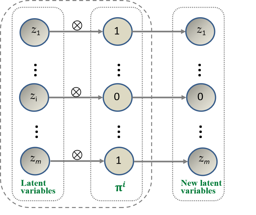
We define $\boldsymbol{\pi}^{i}$ as the $\dim\mathbf{z}$-dimensional row vectors whose elements are ones with zero on the $i$th element and define the ELBO without the $i$th latent variables as

$$E_{Q(\mathbf{z}|\mathbf{x})}\left(\log P(\mathbf{x}|\mathbf{z}\otimes\boldsymbol{\pi}^{i})\right)-\mathcal{KL}[Q(\mathbf{z}\otimes\boldsymbol{\pi}^{i}|\mathbf{x})\parallel P(\mathbf{z}\otimes\boldsymbol{\pi}^{i})],$$

where $P(\mathbf{x}|\mathbf{z}\otimes\boldsymbol{\pi}^{i})$ is defined as

$$P(\mathbf{x}|\mathbf{z}\otimes\boldsymbol{\pi}^{i})=\mathcal{N}(\mathbf{f}(\mathbf{z}\otimes\boldsymbol{\pi}^{i}),\mathbf{I}).$$

Figure 3 visualizes the VAE model without the $i$th latent variable. We should note that we optimize the encoder part and decoder part of ELBO separately in Section 3. It is reasonable to consider two terms in equation (2) separately. So to measure the importance of the $i$th latent variable in decoder and encoder, we subtract original ELBO and ELBO without the $i$th latent variables and add absolute symbol on each term.

$$\bigg{|}E_{Q(\mathbf{z}|\mathbf{x})}\left(\log\frac{P(\mathbf{x}|\mathbf{z})}{P(\mathbf{x}|\mathbf{z}\otimes\boldsymbol{\pi}^{i})}\right)\bigg{|}$$ (7)

$$+ \bigg{|}\mathcal{KL}[Q(\mathbf{z}|\mathbf{x})\parallel P(\mathbf{z})]-\mathcal{KL}[Q(\mathbf{z}\otimes\boldsymbol{\pi}^{i}|\mathbf{x})\parallel P(\mathbf{z}\otimes\boldsymbol{\pi}^{i})]\bigg{|}.$$ (8)

The equation (7) measures the impact of the $i$th latent variable on decoder part of ELBO, and the equation (8) is exactly the increasing of ELBO after we keep the decoder unchanged and marginalize the encoder on the $i$th latent variable. So the bigger the score above is, the more important the $i$th latent variable is.

The equation (8) can be simplified. We discuss it in different types of latent variables. In the mean-field condition, since the latent variables are independent of each other, the $\mathcal{KL}$ divergence can be separated, i.e.,

$$\mathcal{KL}[Q(\mathbf{z}|\mathbf{x})\parallel P(\mathbf{z})]-\mathcal{KL}[Q(\mathbf{z}\otimes\boldsymbol{\pi}^{i}|\mathbf{x})\parallel P(\mathbf{z}\otimes\boldsymbol{\pi}^{i}]$$ (9)

$$= \sum^{\dim\mathbf{z}}_{k=1}\mathcal{KL}[Q(z_{k}|\mathbf{x})\parallel p(z_{k})]-\sum^{\dim\mathbf{z}}_{k=1,k\neq i}\mathcal{KL}[Q(z_{k}|\mathbf{x})\parallel P(z_{k})]$$

$$= \mathcal{KL}[Q(z_{i}|\mathbf{x})\parallel P(z_{i})].$$

However in full-covariance condition, the equation (8) becomes quiet different.

$$\mathcal{KL}[Q(\mathbf{z}|\mathbf{x})\parallel P(\mathbf{z})]-\mathcal{KL}[Q(\mathbf{z}\otimes\boldsymbol{\pi}^{i}|\mathbf{x})\parallel P(\mathbf{z}\otimes\boldsymbol{\pi}^{i})]$$ (10)

$$= E_{Q(\mathbf{z}_{-i}|\mathbf{x})}\left(\mathcal{KL}[Q(z_{i}|\mathbf{z}_{-i},\mathbf{x})\parallel P(z_{i})]\right),$$

where $\mathbf{z}_{-i}$ is $\mathbf{z}$ without the $i$th element and $\dim\mathbf{z}_{-i}=\dim\mathbf{z}-1$. According to the expression of conditional partitioned Gaussian distribution[23], we compute the $\mathcal{KL}[Q(z_{i}|\mathbf{z}_{-i},\mathbf{x})\parallel P(z_{i})]$ using following theorem.

Theorem 5.

Let $(\mathbf{w},\mathbf{u})\sim\mathcal{N}(0,\mathbf{I})$, $(\mathbf{w},\mathbf{u})|\mathbf{x}\sim\mathcal{N}(\boldsymbol{\mu},\boldsymbol{\Sigma})$ where $\boldsymbol{\mu}=(\boldsymbol{\mu}_{\mathbf{w}},\boldsymbol{\mu}_{\mathbf{u}})$. And let

$$\boldsymbol{\Lambda}=\boldsymbol{\Sigma}^{-1}=\begin{pmatrix}\boldsymbol{\Lambda}_{\mathbf{w}\mathbf{w}}&\boldsymbol{\Lambda}_{\mathbf{w}\mathbf{u}}\\ \boldsymbol{\Lambda}_{\mathbf{u}\mathbf{w}}&\boldsymbol{\Lambda}_{\mathbf{u}\mathbf{u}}\end{pmatrix}.$$

Let $\boldsymbol{\Sigma}_{\mathbf{u}|\mathbf{w}}=\boldsymbol{\Lambda}_{\mathbf{u}\mathbf{u}}^{-1}$ and $\boldsymbol{\mu}_{\mathbf{u}|\mathbf{w}}=\boldsymbol{\mu}_{\mathbf{u}}-(\mathbf{w}-\boldsymbol{\mu}_{\mathbf{w}})\boldsymbol{\Lambda}_{\mathbf{w}\mathbf{u}}\boldsymbol{\Sigma}_{\mathbf{u}|\mathbf{w}}$, then

$$\mathcal{KL}[Q(\mathbf{u}|\mathbf{w},\mathbf{x})\parallel P(\mathbf{u})] =\frac{1}{2}\sum^{\dim\mathbf{u}}_{i=1}\left((\boldsymbol{\mu}_{\mathbf{u}|\mathbf{w}})_{i}+(\boldsymbol{\Sigma}_{\mathbf{u}|\mathbf{w}})_{ii}-1\right)$$

$$-\frac{1}{2}\log\det\big{|}\boldsymbol{\Sigma}_{\mathbf{w}\mathbf{w}}\big{|},$$

where $(\boldsymbol{\Sigma}_{\mathbf{u}|\mathbf{w}})_{ii}$ is the $i$th element in diagonal of $\boldsymbol{\Sigma}_{\mathbf{u}|\mathbf{w}}$.

Proof.

The detailed proof can be found in Appendix. ∎

If we want to compute $\mathcal{KL}[Q(z_{i}|\mathbf{z}_{-i},\mathbf{x})\parallel P(z_{i})]$, we only need to let $(\mathbf{w},\mathbf{u})=(\mathbf{z}_{-i},z_{i})$ and $(\boldsymbol{\mu},\boldsymbol{\Sigma})=(\boldsymbol{\mu}(\mathbf{x}),\boldsymbol{\Sigma}(\mathbf{x}))$ in Theorem 5.

Recall that in the weak convergence approximation algorithms, we need $\mathbf{w}$ to be independent of $\mathbf{u}$ as much as possible. Thus according to the definition of mutual information[13], we define the mutual information of the $i$th latent variable as $\mathcal{KL}[Q(\mathbf{z}_{-i},z_{i}|\mathbf{x})\parallel Q(\mathbf{z}_{-i}|\mathbf{x})Q(z_{i}|\mathbf{x})]$. This term measures the amount of information shared by $\mathbf{z}_{-i}$ and $z_{i}$, and is equal to zero if and only if $\mathbf{z}_{-i}$ and $z_{i}$ are independent. So we minus mutual information as a penalty term in full-covariance condition. Furthermore, we have the following theorem,

Theorem 6.

Let mutual information $MI=\mathcal{KL}[Q(\mathbf{z}|\mathbf{x})\parallel Q(\mathbf{w}|\mathbf{x})Q(\mathbf{u}|\mathbf{x})]$, then

$$0\leq E_{Q(\mathbf{w}|\mathbf{x})}\left(\mathcal{KL}[Q(\mathbf{u}|\mathbf{w},\mathbf{x})\parallel P(\mathbf{u})]\right)-MI\leq\mathcal{KL}[Q(\mathbf{z}|\mathbf{x})\parallel P(\mathbf{z})].$$

And maximizing the $E_{Q(\mathbf{w}|\mathbf{x})}\left(\mathcal{KL}[Q(\mathbf{u}|\mathbf{w},\mathbf{x})\parallel P(\mathbf{u})]\right)-MI$ with respect to different choices of $\mathbf{u}$ is equivalent to minimize $E_{Q(\mathbf{u}|\mathbf{x})}\left(\mathcal{KL}[Q(\mathbf{w}|\mathbf{u},\mathbf{x})\parallel P(\mathbf{w})]\right)$.

Proof.

The detailed proof can be found in Appendix. ∎

Since $E_{Q(\mathbf{u}|\mathbf{x})}\mathcal{KL}\left([Q(\mathbf{w}|\mathbf{u},\mathbf{x})\parallel P(\mathbf{w})]\right)$ is zero if and only if $Q(\mathbf{w}|\mathbf{u},\mathbf{x})$ is equal to standard normal distribution $P(\mathbf{w})$ for any $\mathbf{u}$. Thus maximizing $E_{Q(\mathbf{w}|\mathbf{x})}\left(\mathcal{KL}[Q(\mathbf{u}|\mathbf{w},\mathbf{x})\parallel P(\mathbf{u})]\right)-MI$ not only can guarantee the independence of $\mathbf{w}$ and $\mathbf{u}$, but also states that $\mathbf{u}$ contain more information and are more important than $\mathbf{w}$.

Summarizing all the discussion above, we define the evidence lower bound difference (ELBD) score of the $i$th latent variable as

$$\left\{\begin{aligned} &\text{mean-filed}:\bigg{|}E_{Q(\mathbf{z}|\mathbf{x})}\left(\log\frac{P(\mathbf{x}|\mathbf{z})}{P(\mathbf{x}|\mathbf{z}\otimes\boldsymbol{\pi}^{i})}\right)\bigg{|}+\mathcal{KL}[Q(z_{i}|\mathbf{x})\parallel P(z_{i})];\\ &\text{full-covariance}:\bigg{|}E_{Q(\mathbf{z}|\mathbf{x})}\left(\log\frac{P(\mathbf{x}|\mathbf{z})}{P(\mathbf{x}|\mathbf{z}\otimes\boldsymbol{\pi}^{i})}\right)\bigg{|}\\ &\qquad\qquad\qquad+E_{Q(\mathbf{z}_{-i}|\mathbf{x})}\left(\mathcal{KL}[Q(z_{i}|\mathbf{z}_{-i},,\mathbf{x})\parallel P(z_{i})]\right)\\ &\qquad\qquad\qquad-\mathcal{KL}[Q(\mathbf{z}_{-i},z_{i}|\mathbf{x})\parallel Q(\mathbf{z}_{-i}|\mathbf{x})Q(z_{i}|\mathbf{x})].\\ \end{aligned}\right.$$ (11)

Actually, ELBD score in mean-field condition is a special case of ELBD score in full-covariance condition. As all the latent variables are independent in mean-field condition, the mutual information of every latent variable is always zero. Finally, we give the algorithms to compute these two kinds of ELBD scores.

Algorithm 7 Computing all the ELBD scores in mean-field Gaussian posterior condition

0:  data set $\mathbb{D}=\{\mathbf{x}_{1},...,\mathbf{x}_{N}\}$, VAE model

1:  ELBD={};

2:  for $i$ from 1 to $\dim\mathbf{z}$ do

3:     $L=0$, $\mathcal{KL}=0$;

4:     Let $\boldsymbol{\pi}^{i}=(1,1,...,0,...,1)$ where $0$ is the $i$th element;

5:     for  data $\mathbf{x}$ in $\mathbb{D}$ do

6:        $\boldsymbol{\mu}$, $\log\boldsymbol{\sigma}^{2}=EncoderNetwork(\mathbf{x}$);

7:        sample $\boldsymbol{\epsilon}$ from normal distribution $\mathcal{N}(0,\mathbf{I})$

8:        $\mathbf{z}=\boldsymbol{\epsilon}\otimes\exp(\frac{1}{2}\log\boldsymbol{\sigma}^{2})+\boldsymbol{\mu}$;

9:        $\mathbf{x}^{\prime}=DecoderNetwork(\mathbf{z})$;

10:        $\widetilde{\mathbf{x}}=DecoderNetwork(\mathbf{z}\otimes\boldsymbol{\pi}^{i})$;

11:        $L=L+\frac{1}{2}\underset{k=1}{\overset{\dim\mathbf{x}}{\sum}}\left(\big{|}(\mathbf{x}-\mathbf{x}^{\prime})^{2}-(\mathbf{x}-\widetilde{\mathbf{x}})^{2}\big{|}\right)_{k}$;

12:        $kl=\frac{1}{2}\left(\mu^{2}_{i}+\exp(\log\sigma^{2}_{i})-\log\sigma^{2}_{i}-1\right)$

13:        $\mathcal{KL}=\mathcal{KL}+kl$

14:     end for

15:     $ELBD_{i}=(L+\mathcal{KL})/N$;

16:     add $ELBD_{i}$ in the set ELBD;

17:  end for

17:  ELBD

In Algorithm 7 and Algorithm 8, we can only choose a mini-batch of data set as input data set $\mathbb{D}$ to reduce computation. In Algorithm 7, line 11 computes equation (7) of the $i$th latent variable for every pair of original data $\mathbf{x}$ and generated data $\mathbf{x}^{\prime}$, $\widetilde{\mathbf{x}}$. The $L$ is the unbiased estimation of equation (7). Line 12 computes the exact value of equation (9). Adding these two values and divide the number of data, we obtain the unbiased estimation of ELBD in mean-field condition in equation (11) with respect to $Q(\mathbf{z}|\mathbf{x})$.

In Algorithm 8, we also compute the exact value $\mathcal{KL}$ divergence in line 14. However it is the unbiased estimation of equation (10). Meanwhile $L_{1}-L_{2}-L_{3}$ is the unbiased estimation of mutual information where $\boldsymbol{\Sigma}_{-i}$ is covariance matrix that removes the $i$th row and the $i$th column. After all we have the unbiased estimation of ELBD score of the $i$th latent variable under full-covariance condition in line 22.

Algorithm 8 Computing all the ELBD scores in full-covariance Gaussian posterior condition

0:  data set $\mathbb{D}=\{\mathbf{x}_{1},...,\mathbf{x}_{N}\}$, VAE model

1:  ELBD={};

2:  for $i$ from 1 to $\dim\mathbf{z}$ do

3:     $L=0$, $\mathcal{KL}=0$, $MI=0$;

4:     Let $\boldsymbol{\pi}^{i}=(1,1,...,0,...,1)$ where $0$ is the $i$th element;

5:     for  data $\mathbf{x}$ in $\mathbb{D}$ do

6:        $\boldsymbol{\mu}$, $\log\boldsymbol{\sigma}$, $\mathbf{L}_{m}=EncoderNetwork(\mathbf{x}$);

7:        mask matrix $\mathbf{L}_{m}$ and turn the $\mathbf{L}_{m}$ to lower triangular matrix with zeros on and above the diagonal;

8:        $\mathbf{L}=\mathbf{L}_{m}+diag(\exp(\boldsymbol{\sigma}))$;

9:        sample $\boldsymbol{\epsilon}$ from normal distribution $\mathcal{N}(0,\mathbf{I})$

10:        $\mathbf{z}=\boldsymbol{\mu}+\boldsymbol{\epsilon}\mathbf{L}$;

11:        $\mathbf{x}^{\prime}=DecoderNetwork(\mathbf{z})$;

12:        $\widetilde{\mathbf{x}}=DecoderNetwork(\mathbf{z}\otimes\boldsymbol{\pi}^{i})$;

13:        $L=L+\frac{1}{2}\underset{k=1}{\overset{\dim\mathbf{x}}{\sum}}\left(\big{|}(\mathbf{x}-\mathbf{x}^{\prime})^{2}-(\mathbf{x}-\widetilde{\mathbf{x}})^{2}\big{|}\right)_{k}$;

14:        Compute $kl$ using Theorem 5;

15:        $\mathcal{KL}=\mathcal{KL}+kl$;

16:        $\boldsymbol{\Sigma}=\mathbf{L}\mathbf{L}^{\top}$;

17:        $L_{1}=-\frac{1}{2}(\mathbf{z}-\boldsymbol{\mu})\boldsymbol{\Sigma}^{-1}(\mathbf{z}-\boldsymbol{\mu})^{\top}$;

18:        $L_{2}=-\frac{1}{2}(\mathbf{z}_{-i}-\boldsymbol{\mu}_{-i})\boldsymbol{\Sigma}_{-i}^{-1}(\mathbf{z}_{-i}-\boldsymbol{\mu}_{-i})^{\top}$;

19:        $L_{3}=-\frac{1}{2}(z_{i}-\mu_{i})(\boldsymbol{\Sigma})_{ii}^{-1}(z_{i}-\mu_{i})$;

20:        $MI=MI+L_{1}-L_{2}-L_{3}$;

21:     end for

22:     $ELBD_{i}=(L+\mathcal{KL}-MI)/N$;

23:     add $ELBD_{i}$ in the set ELBD;

24:  end for

24:  ELBD

After having ELBD scores for all latent variables, we can decide how many features we need to select begin at the largest ELBD score to the smallest. Then we build zero-one vector $\boldsymbol{\pi}$ by setting the values as zeros correspond to the indices of selected features $\mathbf{u}$ and others as ones.

Besides ELBD, we can use many other feature selection algorithms to build $\boldsymbol{\pi}$. For each data $\mathbf{x}$, we use encoder network and reparameterization to get $\mathbf{z}$, and see $\mathbf{z}$ as a new data. So we turn the data set $\{\mathbf{x}_{1},...,\mathbf{x}_{N}\}$ to $\{\mathbf{z}_{1},...,\mathbf{z}_{N}\}$, and do the feature selection on the new data set. Similarly, we pick the important features and set elements of $\boldsymbol{\pi}$ as zeros with respect to the indices of important features.

We can extend the ELBD score such that ELBD score can not only measure the importance of latent variables in VAE, but can select features on many classification tasks. Now let consider classification task data set $\mathbb{D}_{c}=\{(\mathbf{x}_{1},\mathbf{y}_{1}),...,(\mathbf{x}_{N},\mathbf{y}_{N})\}$. Let $M$ be the model which is already trained on $\mathbb{D}_{c}$ without feature selection process and $M(\mathbf{x})$ is the prediction $M$ makes on data $\mathbf{x}$. The type of $M$ should be the same as the model we want to use on $\mathbb{D}_{c}$ after feature selection process. For example, if we want to use the decision tree model after feature selection, we will choose $M$ as decision tree model and train it on $\mathbb{D}_{c}$ without feature selection process. We define the generalized ELBD (gELBD) score of the $i$th feature as

$$\frac{1}{N}\sum^{N}_{k=1}\left(\big{|}L(\mathbf{y}_{k},\mathbf{y}_{k}^{\prime})-L(\mathbf{y}_{k},\mathbf{y}_{k}^{i})\big{|}\right)+\frac{1}{N}\sum^{N}_{k=1}\sum_{x_{j}\in Val(i)}P(x_{j}|\mathbf{y}_{k})\log\frac{P(x_{j}|\mathbf{y}_{k})}{P(x_{j})},$$ (12)

where $L$ is the loss function which is used during the training process of $M$ and $\mathbf{y}_{k}^{\prime}=M(\mathbf{x}_{k})$, $\mathbf{y}_{k}^{i}=M(\mathbf{x}_{k}\otimes\boldsymbol{\pi}^{i})$. $Val(i)$ is the range that the $i$th feature can take. The probability $P(x_{j})$ stands for the frequency of value $x_{j}$ in $\mathbb{D}_{c}$ and $P(x_{j}|\mathbf{y}_{k})$ represents the frequency of value $x_{j}$ with label $\mathbf{y}_{k}$. Therefore the gELBD can be only used on discrete features with discrete labels and if we want use it on continuous features, some data discretization techniques will be needed beforehand.

Compared to ELBD, gELBD (12) is nearly the copy of equation (7) and (8), and it is same as mean-field condition in equation (11). However gELBD sees $\mathbf{z}$ as original data and $\mathbf{x}$ as label of $\mathbf{z}$, and then $\mathbf{x}^{\prime}$ becomes the prediction of model $M$. And we do not make assumption that every feature is independent of each other. The second term of equation (12) has the equivalent form that

$$\frac{1}{N}\sum^{N}_{k=1}\sum_{x_{j}\in Val(i)}P(x_{j}|\mathbf{y}_{k})\log\frac{P(x_{j}|\mathbf{y}_{k})}{P(x_{j})}$$

$$= \sum_{\mathbf{y}_{k}}P(\mathbf{y}_{k})\sum_{x_{j}\in Val(i)}P(x_{j}|\mathbf{y}_{k})\log\frac{P(x_{j}|\mathbf{y}_{k})}{P(x_{j})},$$

which is also called information gain in other articles[13].

Different from other feature selection scores, ELBD and gELBD need to train models without feature selection process beforehand, and they need the prediction on $\mathbf{x}\otimes\boldsymbol{\pi}^{i}$ for all data $\mathbf{x}$ and $1\leq i\leq\dim\mathbf{z}$. Thus ELBD and gELBD are more complex that they need $O(\dim\mathbf{z}\times N)$ times forward computation of model. However we may see in Section 5 that ELBD and gELBD have better performance than many other features selection algorithms including state-of-the-art feature selection algorithms.

5 Experimental Studies and Discussions

In this section, we use 7 data sets to evaluate our algorithms, including MNIST[24], KMNIST[25], Hands Gestures[26], Fingers[27], Brain[28], Yale[29] and Chest[30]. The basic information about these data sets is listed in Table I. We also provide the values of some hyperparameters in Table I. We use 4 types of VAE: VAE, CVAE, NF-VAE, IAF-VAE, which are mentioned in Section 2, to fit these 7 data sets. Then we choose $\mathbf{u}$ from the latent variables and use algorithms in Section 3 to optimize models under different types of Gaussian posterior, i.e., mean-field and full-covariance. To select important latent variables as $\mathbf{u}$, we apply ELBD algorithm. We also use other 9 feature selection algorithms, Laplacian score (Lap)[15], spectral feature selection (SPEC)[31], multi-cluster feature selection (MCFS)[32], nonnegative discriminative feature selection (NDFS)[33], unsupervised feature selection (UDFS)[34], infinite feature selection (Inf)[35], fisher score (Fisher)[36], efficient and robust feature selection (RFS)[37] and relevant feature selection (ReliefF)[16], to select $\mathbf{u}$ and to compare with ELBD. These 9 algorithms are commonly used and Inf is one of the state-of-the-art feature selection algorithms. Furthermore we get other 5 data sets, Fashion-MNIST[38], EMNIST[39], Shape[40], Chinese Calligraphy[41] and Eyes[42], which are all picture data sets. The basic information about these data sets is also shown in Table IX. Then we use gELBD to do the feature selection on classification task on these data sets and we also use these 9 feature selection algorithms as comparisons. We do all these experiments on GPUs 3060 and 2080Ti with 16G memory. The code of algorithms is available in https://github.com/ronedong/ELBD-Efficient-score-algorithm-for-feature-selection-on-latent-variables-of-VAE

5.1 Optimize results of VAE

TABLE I: Basic information about data sets of generative tasks

Datasets	Number of	Number of pixels	Categories	Train set size vs	Dimension of	Mini-batch	$K$
	pictures	on one picture		Test set size	latent variables	size
MNIST	70000	28$\times$28	10	6:1	50	2000	15
KMNIST	70000	28$\times$28	10	6:1	50	2000	15
Hand Gestures	24000	50$\times$50	20	3:1	100	1000	10
Fingers	21600	64$\times$64	-	5:1	100	600	10
Brain	4600	128$\times$128	2	4:1	150	300	10
Yale	2452	150$\times$150	-	4:1	200	200	10
Chest	5856	150$\times$150	2	8:1	150	200	10

TABLE II: MNIST

Model	Loss	origin	ELBD	Lap	SPEC	MCFS	NDFS	UDFS	Inf	Fisher	RFS	ReliefF
VAE(MF)	-ELBO	69.3(0.93)	31.5(0.53)	32.5(0.38)	32.6(0.43)	57.4(2.72)	64.2(0.80)	32.0(1.07)	31.6(0.45)	31.8(0.43)	38.2(1.51)	31.8(0.47)
	L2	40.5(1.53)	31.3(0.45)	33.3(0.44)	32.3(0.47)	37.2(1.22)	38.1(1.15)	31.5(0.47)	32.9(0.43)	31.7(0.40)	37.9(0.86)	31.7(0.54)
VAE(FC)	-ELBO	29.0(0.12)	5.7(0.09)	20.6(0.17)	16.8(0.55)	9.0(0.85)	6.5(0.29)	12.5(0.90)	11.6(1.24)	5.9(0.16)	6.2(0.08)	8.9(0.83)
	L2	35.6(0.45)	26.5(0.13)	34.9(0.30)	34.4(0.15)	29.6(0.73)	27.2(0.18)	32.4(0.50)	31.4(0.96)	26.6(0.16)	27.0(0.10)	30.2(0.79)
CVAE(MF)	-ELBO	67.0(1.54)	42.4(1.47)	43.4(1.42)	43.4(1.50)	59.2(4.15)	65.9(0.92)	43.5(1.55)	43.4(1.64)	43.5(1.55)	66.2(1.23)	43.6(1.42
	L2	48.5(1.57)	42.4(1.47)	43.3(1.42)	43.3(1.47)	46.1(1.44)	47.9(1.56)	43.3(1.46)	43.3(1.49)	43.3(1.39)	47.9(1.61)	43.4(1.44)
CVAE(FC)	-ELBO	29.2(0.54)	4.2(0.09)	33.3(1.4)	32.4(1.73)	29.5(3.21)	29.4(2.3)	28.8(0.73)	29.0(1.29)	19.9(0.59)	25.9(1.38)	36.9(1.86)
	L2	35.2(0.05)	25.8(0.05)	80.9(2.5)	79.1(2.9)	74.8(6.42)	74.4(4.63)	72.9(1.22)	73.9(2.41)	56.6(0.94)	67.9(2.12)	86.3(3.88)
NF-VAE(MF)	-ELBO	71.8(1.25)	32.4(1.06)	32.5(1.11)	32.4(1.23)	57.0(1.33)	64.9(0.88)	32.6(1.05)	33.0(1.24)	32.4(0.97)	61.0(1.71)	32.8(1.09)
	L2	41.4(1.42)	31.6(0.14)	32.4(1.17)	32.3(1.17)	37.1(1.6)	38.5(1.32)	32.4(1.14)	32.5(1.17)	32.2(1.08)	38.4(1.28)	32.5(1.14)
NF-VAE(FC)	-ELBO	29.1(0.02)	6.3(0.23)	20.7(0.2)	23.3(1.05)	12.0(1.22)	7.6(0.68)	19.1(2.74)	16.5(1.04)	6.5(0.09)	7.6(0.05)	10.2(0.17)
	L2	36.2(0.43)	27.5(0.31)	35.5(0.55)	47.5(2.18)	35.9(2.53)	29.0(0.82)	45.0(4.18)	39.3(2.2)	27.7(0.09)	29.1(0.01)	32.5(0.2)
IAF-VAE(MF)	-ELBO	18.44(0.24)	18.39(0.21)	18.39(0.22)	18.41(0.22)	18.41(0.21)	18.41(0.22)	18.40(0.22)	18.42(0.22)	18.42(0.22)	18.40(0.22)	18.44(0.24)
	L2	18.42(0.22)	18.39(0.22)	18.39(0.22)	18.40(0.22)	18.40(0.21)	18.41(0.23)	18.39(0.21)	18.41(0.23)	18.40(0.21)	18.40(0.22)	18.42(0.22)
IAF-VAE(FC)	-ELBO	14.4(1.03)	7.9(0.96)	8.8(0.73)	8.8(0.77)	8.3(1.0)	8.4(0.77)	8.7(1.2)	8.2(0.93)	8.0(0.93)	8.0(0.95)	8.3(0.9)
	L2	34.2(1.73)	33.4(1.91)	34.0(1.71)	34.0(1.72)	33.7(1.96)	33.7(1.75)	33.9(1.95)	33.6(1.87)	33.4(1.89)	33.4(1.89)	33.6(1.85)

TABLE III: KMNIST

Model	Loss	origin	ELBD	Lap	SPEC	MCFS	NDFS	UDFS	Inf	Fisher	RFS	ReliefF
VAE(MF)	-ELBO	149.4(1.59)	99.8(2.05)	110.2(1.16)	107.9(1.36)	106.5(4.68)	115.5(1.65)	105.3(1.25)	101.7(2.09)	100.5(1.68)	104.4(3.53)	99.8(1.89)
	L2	99.7(1.69)	87.5(1.57)	88.6(1.67)	88.9(2.09)	88.6(2.28)	89.0(1.83)	88.44(2.01)	88.4(1.75)	88.0(1.9)	88.9(2.15)	87.5(2.07)
VAE(FC)	-ELBO	67.2(0.09)	41.2(0.17)	46.9(0.14)	43.5(0.42)	41.5(0.22)	41.2(0.35)	43.8(0.34)	46.3(0.41)	40.5(0.11)	41.0(0.15)	43.6(0.5)
	L2	93.6(0.25)	84.7(0.29)	84.7(0.52)	84.5(0.6)	83.5(0.63)	83.7(0.48)	84.4(0.8)	84.7(0.58)	83.4(0.68)	83.9(0.51)	84.8(0.6)
CVAE(MF)	-ELBO	161.8(0.65)	127.0(0.6)	127.3(0.64)	127.3(0.6)	150.0(3.35)	159.8(1.03)	127.3(0.58)	127.5(0.64)	127.8(1.23)	160.9(1.08)	127.9(0.62)
	L2	136.7(1.77)	126.9(0.56)	127.3(0.68)	127.2(0.55)	132.6(1.72)	135.3(1.16)	127.3(0.66)	127.4(0.65)	127.4(0.96)	135.5(1.54)	126.9(0.68)
CVAE(FC)	-ELBO	84.1(0.15)	68.3(0.16)	90.3(0.86)	91.3(1.07)	83.2(0.15)	80.3(2.79)	86.9(1.89)	82.6(1.68)	82.0(2.04)	87.6(1.33)	84.9(1.4)
	L2	159.9(0.39)	156.8(0.31)	193.6(1.5)	195.8(1.51)	181.3(0.36)	176.2(5.22)	188.2(3.96)	181.0(3.35)	179.3(3.53)	190.5(2.52)	182.5(1.98)
NF-VAE(MF)	-ELBO	152.7(0.82)	103.1(0.9)	114.6(1.1)	112.0(0.73)	109.1(1.81)	117.1(0.45)	106.8(1.15)	105.9(0.71)	104.7(0.73)	107.1(0.75)	103.2(0.46)
	L2	103.6(0.8)	90.6(0.86)	92.2(1.0)	92.1(1.39)	90.8(1.04)	92.0(1.35)	90.7(0.27)	90.8(0.85)	91.6(0.9)	91.2(0.64)	99.7(0.39)
NF-VAE(FC)	-ELBO	67.2(0.09)	41.2(0.2)	46.8(0.15)	47.3(1.68)	43.3(0.84)	42.2(0.43)	46.5(1.56)	46.4(0.15)	42.9(0.21)	43.4(0.18)	45.1(0.5)
	L2	93.7(0.29)	84.7(0.29)	85.2(0.38)	92.5(2.65)	87.5(1.32)	85.6(0.47)	90.6(3.78)	85.2(0.35)	86.2(0.49)	86.8(0.39)	88.4(1.02)
IAF-VAE(MF)	-ELBO	88.7(0.77)	84.8(0.03)	85.8(0.78)	85.7(0.84)	88.0(1.03)	88.7(0.97)	85.8(0.77)	85.9(0.76)	85.8(0.93)	89.0(1.04)	85.4(0.85)
	L2	81.4(0.93)	77.9(0.88)	78.3(0.85)	78.3(0.95)	80.6(1.14)	81.4(1.03)	78.3(0.83)	78.4(0.8)	78.3(0.92)	81.3(1.01)	77.9(0.85)
IAF-VAE(FC)	-ELBO	61.2(1.35)	50.7(1.64)	55.4(1.71)	55.4(1.66)	52.6(0.99)	51.4(1.43)	53.6(2.01)	51.0(1.64)	51.4(0.93)	52.5(1.45)	50.9(1.61)
	L2	121.4(3.16)	118.2(3.28)	121.1(3.29)	121.1(3.27)	119.5(2.99)	118.9(3.17)	120.1(3.5)	118.6(3.28)	118.9(2.85)	119.7(3.18)	118.6(3.26)

TABLE IV: Hand Gestures

Model	Loss	origin	ELBD	Lap	SPEC	MCFS	NDFS	UDFS	Inf	Fisher	RFS	ReliefF
VAE(MF)	-ELBO	161.5(3.12)	122.4(4.38)	122.9(4.05)	123.1(4.08)	137.4(4.97)	138.1(3.58)	123.1(4.2)	123.2(4.55)	122.9(4.02)	158.6(3.79)	123.1(4.17)
	L2	133.7(3.44)	121.4(4.68)	122.6(4.13)	122.8(4.11)	126.5(4.05)	126.6(3.18)	122.9(4.32)	123.3(4.48)	123.2(4.51)	130.6(2.84)	122.9(4.16)
VAE(FC)	-ELBO	65.8(1.44)	41.7(1.75)	107.6(30.77)	143.1(16.18)	135.5(27.32)	84.8(24.86)	129.4(15.61)	150.7(23.93)	43.7(1.28)	46.7(1.82)	75.4(11.73)
	L2	123.5(4.19)	116.5(3.57)	236.2(63.74)	306.3(31.73)	298.3(53.24)	199.6(52.16)	286.5(29.99)	323.7(48.23)	119.7(3.0)	125.2(2.34)	179.9(21.97)
CVAE(MF)	-ELBO	154.0(2.01)	118.6(1.56)	119.1(1.29)	119.2(1.53)	127.7(4.84)	135.3(2.34)	120.5(2.19)	119.2(1.56)	119.1(1.5)	150.4(1.97)	151.9(2.58)
	L2	129.2(1.47)	118.4(1.39)	118.9(1.72)	118.9(1.48)	121.3(2.47)	122.6(2.01)	119.0(1.15)	118.9(1.48)	118.7(1.24)	125.7(1.97)	127.8(2.64)
CVAE(FC)	-ELBO	61.6(0.44)	38.3(0.61)	127.8(7.03)	114.0(13.49)	123.3(6.57)	123.8(8.53)	103.1(24.01)	112.7(17.12)	41.1(1.04)	43.2(0.78)	100.9(7.49)
	L2	116.9(0.93)	110.5(1.03)	281.1(15.32)	255.2(26.84)	276.1(14.11)	273.0(14.43)	234.6(46.61)	247.4(34.47)	115.0(1.81)	118.6(1.53)	229.3(15.65)
NF-VAE(MF)	-ELBO	163.0(1.89)	124.1(1.16)	124.6(1.18)	124.6(1.26)	135.5(10.65)	138.3(3.65)	124.2(1.31)	124.7(1.25)	124.6(1.02)	160.5(1.97)	124.6(0.96)
	L2	134.1(2.15)	123.9(1.25)	124.2(1.39)	123.9(1.16)	126.3(2.74)	127.3(2.07)	124.2(1.27)	124.3(1.36)	124.4(1.1)	133.4(2.09)	124.0(1.1)
NF-VAE(FC)	-ELBO	65.5(0.2)	41.0(0.56)	130.8(2.14)	145.7(15.41)	133.5(10.64)	86.3(16.38)	127.3(24.23)	129.4(2.86)	43.0(0.19)	50.0(2.73)	78.5(18.41)
	L2	122.3(0.95)	115.3(0.98)	284.2(6.98)	316.4(32.14)	296.0(20.68)	200.5(33.42)	278.9(46.28)	287.3(2.8)	118.4(0.14)	130.8(5.31)	185.4(35.19)
IAF-VAE(MF)	-ELBO	133.0(2.28)	126.0(2.69)	126.1(2.74)	126.1(2.68)	130.5(1.97)	128.4(2.52)	126.1(2.7)	126.0(2.73)	126.5(2.75)	132.5(2.28)	126.1(2.62)
	L2	128.4(2.69)	126.0(2.72)	126.0(2.7)	126.1(2.74)	127.6(2.45)	126.8(2.67)	126.1(2.7)	126.1(2.66)	126.0(2.79)	128.4(2.67)	126.1(2.75)
IAF-VAE(FC)	-ELBO	58.7(3.75)	41.7(3.63)	43.8(4.49)	42.8(4.81)	45.3(3.69)	48.7(4.39)	43.7(2.61)	48.9(4.3)	42.1(3.65)	41.9(3.57)	48.3(4.23)
	L2	120.5(7.13)	118.0(7.22)	120.6(8.76)	119.8(9.25)	121.0(7.02)	122.6(8.34)	119.8(6.49)	122.3(8.74)	118.3(7.21)	118.2(7.25)	122.0(8.68)

TABLE V: Fingers

Model	Loss	origin	ELBD	Lap	SPEC	MCFS	NDFS	UDFS	Inf	Fisher	RFS	ReliefF
VAE(MF)	-ELBO	52.7(0.9)	30.0(0.51)	30.0(0.49)	29.8(0.61)	39.3(3.52)	30.1(0.51)	31.1(1.57)	29.8(0.48)	30.2(0.32)	37.9(2.24)	51.6(0.88)
	L2	35.2(0.85)	29.7(0.48)	29.8(0.46)	29.9(0.37)	31.7(1.08)	30.0(0.61)	29.9(0.51)	29.7(0.41)	29.9(0.42)	31.7(0.69)	34.6(1.02)
VAE(FC)	-ELBO	14.7(0.08)	12.6(0.25)	19.1(1.21)	19.6(0.28)	17.8(1.39)	17.8(0.47)	18.8(0.91)	17.1(0.81)	14.0(0.67)	17.4(1.41)	18.6(0.46)
	L2	28.1(0.28)	23.9(0.43)	36.4(2.52)	37.9(0.76)	34.3(2.95)	34.0(1.12)	36.3(1.97)	32.5(1.55)	26.4(1.29)	33.3(2.85)	35.8(0.68)
NF-VAE(MF)	-ELBO	52.1(0.74)	29.0(0.11)	29.1(0.13)	29.2(0.2)	36.3(2.04)	29.2(0.26)	30.0(0.85)	29.0(0.27)	31.3(1.68)	36.6(3.3)	51.2(0.54)
	L2	34.3(0.35)	28.9(0.26)	28.9(0.15)	29.0(0.23)	30.1(0.37)	29.1(0.19)	29.1(0.13)	28.9(0.18)	29.3(0.38)	30.4(0.86)	33.5(0.18)
NF-VAE(FC)	-ELBO	14.0(0.06)	12.8(0.09)	19.3(1.36)	19.1(1.09)	18.3(0.47)	17.7(0.93)	18.6(1.12)	17.9(0.99)	15.5(0.41)	16.8(0.55)	19.1(0.25)
	L2	28.2(0.17)	24.2(0.35)	37.5(2.67)	37.1(2.05)	35.3(1.22)	34.1(1.79)	36.0(2.19)	34.4(1.76)	29.7(0.57)	32.3(1.11)	37.1(0.47)
IAF-VAE(MF)	-ELBO	12.42(0.02)	12.35(0.08)	12.36(0.08)	12.36(0.08)	12.36(0.08)	12.36(0.08)	12.36(0.08)	12.36(0.08)	12.36(0.08)	12.35(0.08)	12.36(0.08)
	L2	12.42(0.02)	12.35(0.08)	12.35(0.08)	12.35(0.08)	12.35(0.08)	12.35(0.08)	12.35(0.08)	12.35(0.08)	12.35(0.08)	12.35(0.08)	12.36(0.08)
IAF-VAE(FC)	-ELBO	7.5(0.96)	6.9(0.8)	7.2(0.93)	7.1(0.92)	7.1(0.96)	7.1(0.75)	7.3(0.89)	7.2(0.75)	7.0(0.81)	7.2(0.87)	7.2(1.03)
	L2	26.4(0.91)	25.3(0.6)	25.7(0.91)	25.7(0.77)	25.9(0.92)	25.6(0.39)	26.1(0.73)	25.9(0.64)	25.4(0.6)	25.9(0.73)	25.8(0.87)

TABLE VI: Brain

Model	Loss	origin	ELBD	Lap	SPEC	MCFS	NDFS	UDFS	Inf	Fisher	RFS	ReliefF
VAE(MF)	-ELBO	695.9(8.82)	529.2(13.85)	529.4(13.51)	530.1(14.19)	541.3(15.0)	562.6(11.19)	530.8(13.04)	530.0(13.7)	550.6(15.56)	539.8(13.45)	568.8(18.94)
	L2	565.1(13.68)	527.5(14.2)	528.0(14.21)	528.9(13.69)	530.3(13.95)	533.4(13.59)	529.6(13.57)	528.9(13.8)	531.3(13.99)	530.4(13.74)	534.6(14.82)
VAE(FC)	-ELBO	424.3(9.11)	373.9(10.99)	414.8(7.02)	409.6(4.44)	399.5(15.57)	400.6(7.64)	401.6(20.67)	402.4(9.54)	400.0(15.22)	411.7(13.73)	390.1(13.11)
	L2	796.8(19.81)	783.4(22.10)	861.9(17.05)	857.0(7.29)	835.8(31.86)	840.2(15.49)	841.1(37.92)	844.0(20.18)	836.4(33.03)	867.0(28.5)	818.0(26.95)
CVAE(MF)	-ELBO	689.1(8.36)	527.1(6.68)	527.4(6.87)	527.6(6.96)	541.5(3.7)	567.9(2.74)	530.0(4.11)	527.9(6.57)	548.2(7.35)	539.1(6.29)	572.7(4.58)
	L2	562.5(7.31)	525.1(7.19)	526.6(6.92)	526.4(6.55)	528.8(6.7)	533.7(6.47)	526.5(6.45)	526.5(6.91)	529.0(6.81)	528.3(7.07)	533.5(5.97)
CVAE(FC)	-ELBO	413.1(3.04)	356.6(1.98)	400.7(8.16)	397.6(3.25)	380.2(7.55)	381.1(1.65)	382.7(3.81)	400.7(4.86)	377.0(7.93)	388.6(6.63)	383.4(7.35)
	L2	771.4(6.94)	750.1(4.27)	842.5(13.73)	837.0(3.28)	797.7(16.8)	800.7(6.13)	802.8(6.89)	840.0(9.97)	792.9(15.19)	812.2(12.94)	807.1(15.95)
NF-VAE(MF)	-ELBO	694.6(3.33)	530.1(3.85)	531.1(4.63)	531.6(3.92)	543.8(10.38)	577.3(3.4)	532.1(4.49)	531.9(4.94)	551.7(4.29)	549.0(3.83)	571.6(4.86)
	L2	567.8(3.4)	529.1(4.6)	530.4(4.34)	530.9(4.07)	532.6(5.43)	538.2(3.96)	530.3(4.76)	530.6(5.18)	534.4(4.57)	533.8(3.76)	537.2(3.81)
NF-VAE(FC)	-ELBO	421.2(2.87)	369.7(2.93)	407.7(2.03)	403.6(5.54)	389.7(6.6)	391.3(5.83)	389.8(3.99)	406.7(2.44)	385.3(1.78)	408.3(2.78)	383.2(1.07)
	L2	789.8(6.22)	775.8(4.76)	852.9(6.51)	848.0(18.3)	817.6(12.16)	824.3(14.69)	817.5(6.23)	852.8(8.91)	805.8(1.01)	853.0(6.5)	806.6(3.11)
IAF-VAE(MF)	-ELBO	626.7(19.02)	552.1(11.79)	547.3(17.93)	547.2(17.84)	550.4(20.03)	586.1(25.6)	548.0(18.86)	547.5(17.68)	553.5(20.13)	549.1(19.39)	575.9(22.71)
	L2	562.7(18.11)	546.9(17.78)	547.5(18.21)	547.7(18.3)	548.1(18.46)	554.6(19.53)	547.5(18.24)	547.3(18.22)	548.6(18.9)	547.9(18.18)	553.9(19.48)
IAF-VAE(FC)	-ELBO	367.4(2.38)	312.9(2.59)	323.8(1.46)	323.6(0.62)	319.7(2.42)	327.7(2.37)	326.5(1.27)	338.0(1.48)	320.5(3.49)	318.5(1.99)	313.5(2.56)
	L2	704.0(2.66)	682.6(3.69)	693.2(3.22)	693.3(2.43)	689.3(1.08)	691.3(1.26)	692.1(2.32)	699.8(1.93)	689.4(2.56)	686.8(3.9)	684.5(3.89)

TABLE VII: Yale

Model	Loss	origin	ELBD	Lap	SPEC	MCFS	NDFS	UDFS	Inf	Fisher	RFS	ReliefF
VAE(MF)	-ELBO	355.2(3.46)	236.2(2.73)	285.5(4.83)	284.3(4.37)	274.5(8.64)	239.3(2.39)	236.6(2.52)	235.0(1.95)	299.1(9.88)	268.5(7.84)	326.7(3.12)
	L2	261.5(5.01)	229.6(2.99)	239.3(3.73)	238.2(2.59)	234.6(3.71)	229.4(4.97)	229.3(4.22)	228.3(3.5)	238.9(3.27)	235.0(2.45)	241.9(2.27)
VAE(FC)	-ELBO	192.2(10.58)	145.9(11.17)	178.3(13.23)	178.7(15.1)	223.3(9.88)	173.6(18.51)	235.4(17.83)	196.5(8.38)	159.2(8.56)	227.2(12.79)	214.6(25.94)
	L2	348.3(19.3)	334.9(19.47)	395.3(26.48)	390.6(26.63)	482.7(15.59)	390.6(34.49)	521.2(27.56)	436.2(13.66)	353.5(18.24)	487.9(20.11)	476.7(56.13)
NF-VAE(MF)	-ELBO	354.8(1.57)	232.5(3.41)	277.0(5.81)	283.0(2.47)	270.8(7.93)	236.9(3.1)	235.8(5.25)	233.1(5.24)	291.5(4.66)	271.1(3.8)	324.7(1.01)
	L2	254.3(3.15)	222.6(4.14)	233.1(5.44)	234.8(3.44)	232.5(4.81)	226.2(3.3)	227.6(3.53)	226.3(4.65)	234.9(4.63)	234.4(3.54)	240.9(5.02)
NF-VAE(FC)	-ELBO	172.6(2.34)	131.1(2.75)	182.9(10.96)	168.5(5.74)	231.5(20.21)	156.7(1.69)	210.3(2.06)	173.6(8.67)	144.0(1.07)	237.8(8.15)	235.0(5.06)
	L2	312.5(3.43)	305.9(6.05)	403.2(23.45)	374.0(13.99)	497.5(38.44)	358.6(1.86)	462.7(7.98)	387.3(18.14)	324.9(2.21)	514.0(9.87)	509.5(6.08)
IAF-VAE(MF)	-ELBO	312.7(8.66)	247.7(10.18)	282.1(8.69)	280.2(7.46)	275.7(9.14)	251.6(9.68)	251.6(6.77)	249.3(10.0)	292.8(10.18)	272.3(5.37)	312.1(9.03)
	L2	261.7(7.61)	247.6(9.77)	255.2(10.24)	255.6(10.08)	254.1(8.98)	249.9(9.83)	250.0(8.8)	249.4(10.23)	256.5(9.3)	253.3(7.66)	263.2(9.2)
IAF-VAE(FC)	-ELBO	158.7(5.24)	112.3(3.94)	121.1(6.35)	122.2(5.14)	124.3(5.63)	134.1(5.07)	131.6(6.16)	133.3(2.36)	134.6(6.13)	126.9(7.34)	117.5(6.88)
	L2	303.5(9.12)	287.7(7.03)	296.2(9.29)	297.2(9.49)	298.9(9.34)	305.1(9.8)	302.1(8.57)	303.7(9.67)	304.4(10.91)	299.9(10.72)	294.2(11.04)

TABLE VIII: Chest

Model	Loss	origin	ELBD	Lap	SPEC	MCFS	NDFS	UDFS	Inf	Fisher	RFS	ReliefF
VAE(MF)	-ELBO	642.2(1.6)	519.4(3.35)	519.7(2.77)	519.9(3.09)	538.7(10.61)	600.4(4.31)	520.9(3.69)	520.2(4.02)	552.2(1.99)	524.0(2.45)	580.4(3.84)
	L2	546.4(3.42)	517.8(3.12)	518.3(3.12)	518.7(2.77)	521.1(3.77)	532.1(1.27)	519.0(2.7)	518.6(2.23)	525.2(2.27)	518.9(1.91)	528.9(2.09)
VAE(FC)	-ELBO	296.7(1.77)	249.6(1.61)	323.3(4.8)	319.8(5.78)	313.7(5.89)	308.1(14.7)	318.4(5.9)	316.8(6.14)	301.5(9.59)	314.2(10.67)	311.1(9.29)
	L2	561.0(1.07)	549.8(2.67)	687.9(3.75)	682.7(12.94)	675.4(14.08)	657.8(23.61)	683.6(11.87)	677.4(17.59)	647.2(19.92)	673.4(24.64)	663.8(14.76)
CVAE(MF)	-ELBO	658.9(6.12)	536.1(5.26)	537.7(5.71)	535.7(5.04)	549.7(3.28)	620.7(8.76)	537.7(5.87)	536.8(5.4)	573.0(3.25)	543.9(3.83)	599.6(7.12)
	L2	561.0(6.54)	534.1(5.43)	535.0(5.66)	536.0(5.14)	537.6(4.58)	549.5(5.96)	535.0(5.2)	534.8(5.61)	541.7(5.65)	535.8(4.86)	544.5(6.31)
CVAE(FC)	-ELBO	297.4(1.42)	250.7(1.2)	314.7(3.94)	315.2(3.99)	318.0(7.72)	303.0(10.62)	311.8(9.71)	316.6(3.16)	310.8(8.2)	308.9(6.78)	312.9(2.08)
	L2	561.3(2.73)	552.1(0.97)	668.9(12.21)	670.7(3.54)	673.9(17.31)	651.2(23.32)	666.6(20.12)	678.4(10.82)	667.1(16.86)	660.1(7.43)	668.8(3.77)
NF-VAE(MF)	-ELBO	646.2(3.57)	523.3(3.09)	524.1(2.45)	525.1(3.17)	544.5(4.98)	611.3(2.04)	525.3(2.8)	523.9(3.48)	559.9(7.96)	530.0(4.34)	578.7(8.35)
	L2	547.1(3.63)	522.5(3.20)	523.3(3.03)	522.5(3.51)	525.5(2.6)	535.9(3.11)	522.5(2.96)	522.7(2.98)	527.7(5.0)	523.7(2.99)	531.2(3.05)
NF-VAE(FC)	-ELBO	270.3(0.86)	228.0(1.79)	272.5(6.96)	270.8(3.51)	278.9(3.04)	256.4(4.7)	271.4(2.65)	277.3(3.23)	272.4(4.07)	281.7(1.81)	277.6(0.56)
	L2	507.9(2.76)	506.3(1.74)	585.0(10.71)	581.9(7.36)	602.8(10.68)	554.9(7.48)	587.2(2.58)	602.8(5.41)	587.3(5.97)	604.4(2.96)	596.6(3.7)
IAF-VAE(MF)	-ELBO	652.0(9.45)	588.7(5.33)	591.6(5.23)	591.6(5.51)	600.7(8.95)	646.5(11.27)	591.3(5.67)	591.8(5.49)	616.8(4.68)	593.9(5.47)	633.8(4.55)
	L2	600.0(5.95)	588.6(5.35)	591.2(5.41)	591.8(5.18)	592.1(5.98)	599.8(5.95)	591.5(5.28)	591.3(5.31)	594.9(5.37)	591.9(5.4)	597.4(5.41)
IAF-VAE(FC)	-ELBO	333.4(1.67)	287.2(2.89)	295.3(2.93)	292.0(2.94)	304.5(2.92)	310.3(2.46)	302.5(2.5)	312.2(1.2)	294.4(1.46)	295.3(0.24)	295.3(2.23)
	L2	651.7(5.03)	642.7(5.64)	651.4(2.44)	649.5(4.28)	653.7(3.89)	653.1(4.01)	651.3(4.31)	655.3(3.73)	649.2(4.21)	650.4(2.98)	651.0(2.46)

TABLE IX: Basic information about data sets of classification tasks

Data set	Number of	Number of pixels	Categories	Training set size vs
	pictures	on one picture		Testing set size
Fashion-MNIST	70000	28$\times$28	10	6:1
EMNIST	1456000	28$\times$28	26	6:1
Shape	27292	32$\times$32	4	4:1
Chinese Calligraphy	105029	32$\times$32	20	4:1
Eyes	11525	3$\times$28$\times$28	2	4:1

TABLE X: Accuracy on data set of classification tasks

Data set	gELBD	Lap	SPEC	MCFS	NDFS	UDFS	Inf	Fisher	RFS	ReliefF
Fashion-MNIST	0.872(0.001)	0.870(0.002)	0.869(0.002)	0.836(0.004)	0.838(0.001)	0.869(0.005)	0.834(0.002)	0.872(0.002)	0.867(0.004)	0.867(0.002)
EMNIST	0.909(0.002)	0.835(0.004)	0.861(0.001)	0.852(0.002)	0.905(0.002)	0.905(0.001)	0.853(0.003)	0.908(0.002)	0.893(0.003)	0.907(0.001)
Shape	0.883(0.005)	0.819(0.008)	0.821(0.008)	0.848(0.010)	0.812(0.004)	0.882(0.004)	0.840(0.012)	0.864(0.005)	0.863(0.010)	0.865(0.011)
Chinese Calligraphy	0.806(0.003)	0.745(0.001)	0.785(0.007)	0.748(0.001)	0.799(0.002)	0.795(0.001)	0.787(0.002)	0.800(0.003)	0.786(0.005)	0.779(0.005)
Eyes	0.860(0.008)	0.839(0.016)	0.847(0.012)	0.838(0.006)	0.843(0.008)	0.852(0.005)	0.851(0.017)	0.842(0.003)	0.845(0.006)	0.846(0.011)

Figure 4: (a) The CVAE model on Hand Gestures data set under mean-field condition (b) The CVAE model on Hand Gestures data set under full-covariance condition (c) The NF-VAE model on Fingers data set under mean-field condition (d) The NF-VAE model on Finger data set under full-covariance condition (e) The IAF-VAE model on Yale data set under mean-field condition (f) The IAF-VAE model on Yale data set under full-covariance condition.

In this subsection, we mainly use the marginalization of encoder algorithms and the weak convergence approximation algorithms in Section 3 to optimize VAE and its variants.

Firstly, we give some information about data sets and part of hyperparameters used in these data sets in Table I. The “Categories” term means how many types of labels in the data sets where Fingers and Yale do not have labels. We split each data set into train set and test set randomly. The ratios are shown in “Train set vs Test set” term. The “Dimension of latent variables” term means the dimension of $\mathbf{z}$ used on all the models under this data set, i.e., latent variables of VAE and variants have the same dimension under one data set. Considering the capacity of memory and complexity, we choose a mini-batch of data set to compute feature selection scores for latent variables. The sizes of the mini-batch are listed in term “Mini-batch size”. We also use the same size of mini-batch on all the feature selection algorithms in one data set. The term “$K$” is the hyperparameter in Algorithm 5 and Algorithm 6. We choose “Mini-batch size” and “$K$” as much large as we can because of Corollary 1.

Data sets with labels, MNIST, KMNIST, Hand Gestures, Chest, Brain, are used to test the algorithms on VAE, CVAE, NF-VAE and IAF-VAE each under two types of latent variables totally 8 models. Because CVAE is a supervised model, data sets without labels, Fingers and Yale, are tested only on VAE, NF-VAE and IAF-VAE each under two types of latent variables totally 6 models. We use full connect neural networks on data sets MNIST, KMNIST, and convolutional neural networks on data sets Hand Gestures, Fingers, Brain, Yale and Chest to build the encoder networks and decoder networks. We use negative ELBO as the loss function for all models and use Adam algorithm[43] to minimize the loss. The learning rate is in $[1\times 10^{-3},1\times 10^{-5}]$.

Considering the marginalization of encoder is rather help to generate pictures but give a mathematical explanation of ELBO after optimization, we use negative ELBO and L2 two kinds of losses to measure the results of models on test data set but only use negative ELBO in training steps. The decreasing of both losses can state that our algorithms do generate much more clear pictures

The whole experiments run as follow: Firstly, we train the VAE or its variants without feature selection, and obtain a trained original model $M$. Secondly, for ELBD, we directly use Algorithm 7 or Algorithm 8 to compute the score of every latent variable. For other feature selection algorithms, we turn data set $\{\mathbf{x}_{1},...,\mathbf{x}_{N}\}$ to set of latent variables $\{\mathbf{z}_{1},...,\mathbf{z}_{N}\}$ by using encoder in $M$. We see the $\{\mathbf{z}_{1},...,\mathbf{z}_{N}\}$ as new data set and use other 9 algorithms on it to obtain the scores for every latent variable. Thirdly, we pick the $60\%$ of latent variables which have the largest feature selection scores and see them as $\mathbf{u}$. Then we build $\boldsymbol{\pi}$ by the rule that $\pi_{i}$ is zero if $i$ is one of the indices that we pick and is one otherwise. Different feature selection algorithm generates different $\mathbf{u}$ and $\boldsymbol{\pi}$. Finally, we put $\boldsymbol{\pi}$, $M$ and $K$ into Algorithm 3, Algorithm 5 if latent variables of $M$ have mean-field Gaussian posterior or Algorithm 4, Algorithm 6 if latent variables of $M$ have full-covariance Gaussian posterior to optimize $M$. Using the new pictures generated by the weak convergence algorithms, we can compute the first term of ELBO (2). Combing the $\mathcal{KL}$ divergence from Algorithm 3 or Algorithm 4, we have the ELBO of model after optimization. Combing the generated pictures and original pictures, we have the L2 loss of model after optimization.

Table 2 to Table 8 are the results on 7 data sets in Table I. The titles of them state the data set we run our experiments on. In each table, MF stands for mean-field and FC stands for full-covariance. For example, VAE(MF) means VAE model with mean-field Gaussian posterior. Every column uses one feature selection algorithm to generate $\boldsymbol{\pi}$ for different models. Every row uses different feature selection algorithms to compute $\boldsymbol{\pi}$ for one model where “origin” term shows the results of original models without any optimization algorithms. We train three models with different random seeds in each kind of model in each data set. We list mean and standard deviation of the three models as the form that mean(standard deviation) in each entry. The lowest result in each row is bold.

Analyzing the Table 2 to Table 8, we find that most of the feature selection algorithms can optimize the models compare to the results in “origin” and all the models can be optimized. Moreover, in most of the cases, the optimized results are tremendous. For example, in Yale data set Table VII, the optimized result of VAE(MF) by ELBD is $33.5\%$ less than original result with respect to -ELBO loss and $12.2\%$ with respect to L2 loss. The optimized result (236.2) is even smaller than the result of original state-of-the-art model IAF-VAE(MF) (312.7). It states that our optimization algorithms in Section 3 are very effective and can be used on many variants of VAE. Compared to other 9 feature selection algorithms, ELBD has the best optimized results in almost any cases. Some algorithms can not even have optimized effect. For example, CVAE(FC) optimized by ReliefF in MNIST data set has -ELBO loss (36.9) which is bigger than the original result (29.2). Recalling the analysis in the end of Section 3, i.e., the more important selected latent variables are, the better optimized result is, we also can derive that ELBD is better in picking important latent variables than other 9 algorithms.

Figure 5: (a) (b) (c) are original pictures in Yale data set. (d) (e) (f) are pictures generated by VAE(MF). (g) (h) (i) are pictures generated by VAE(MF) optimized by the weak convergence approximation algorithm under ELBD.

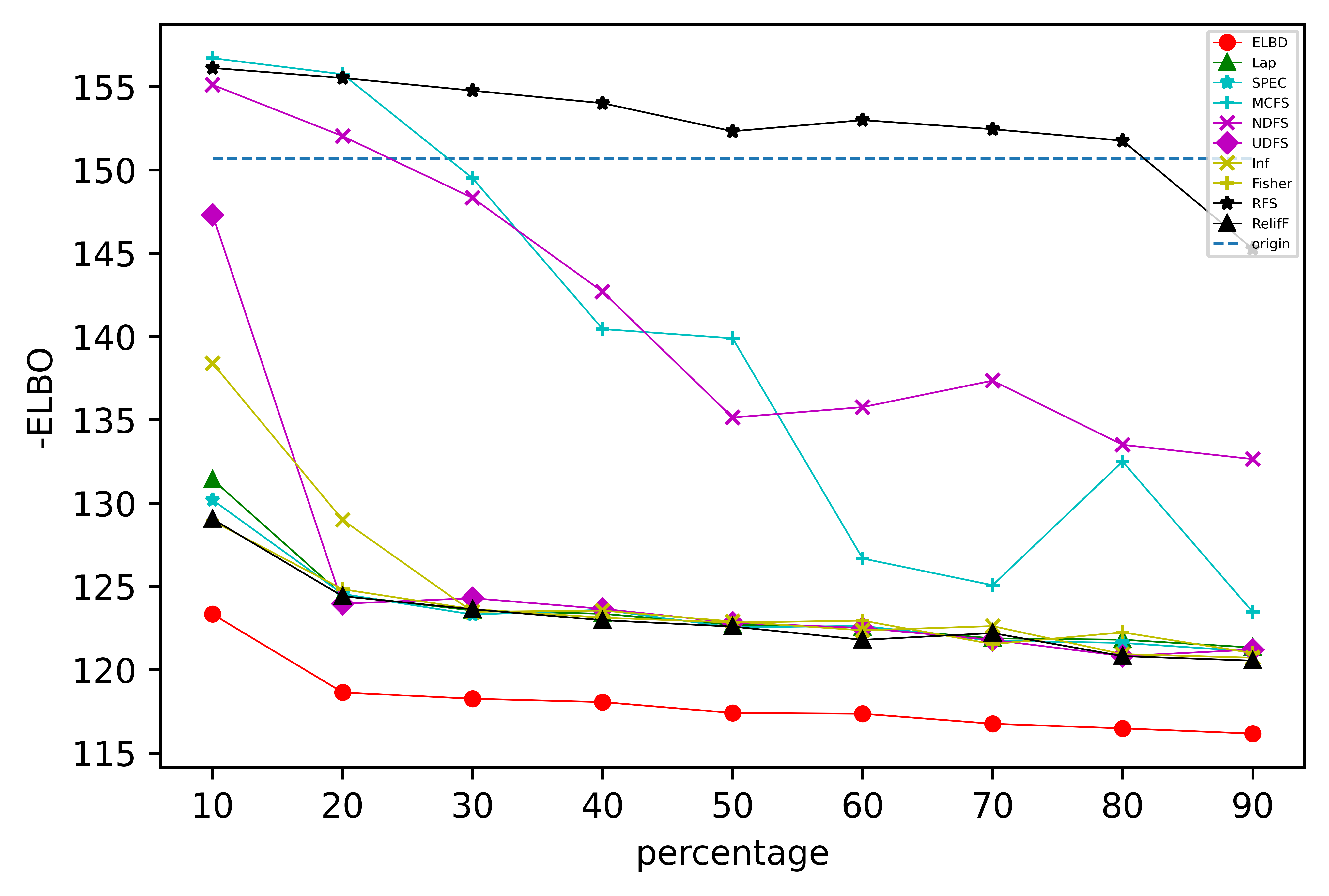
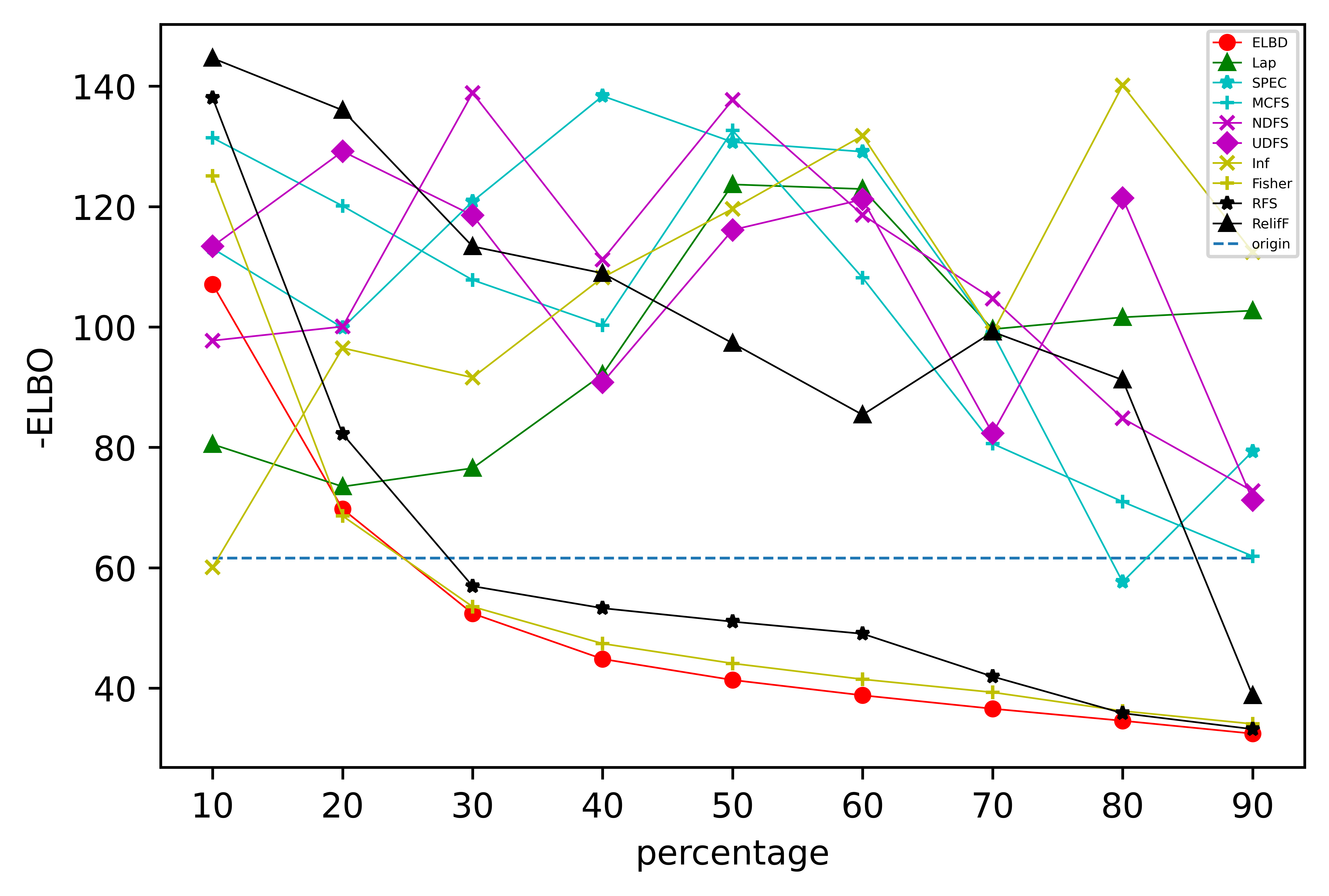
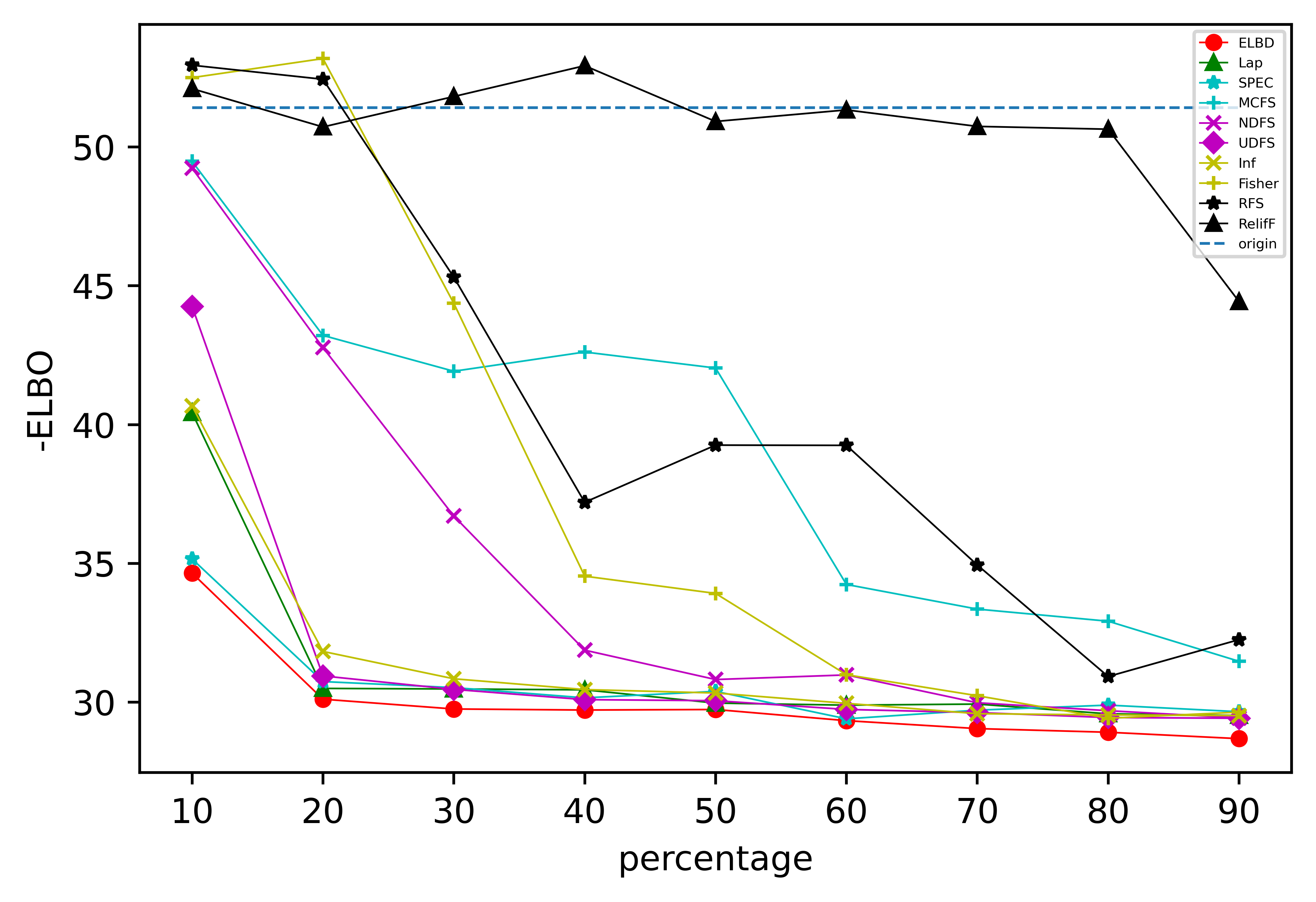
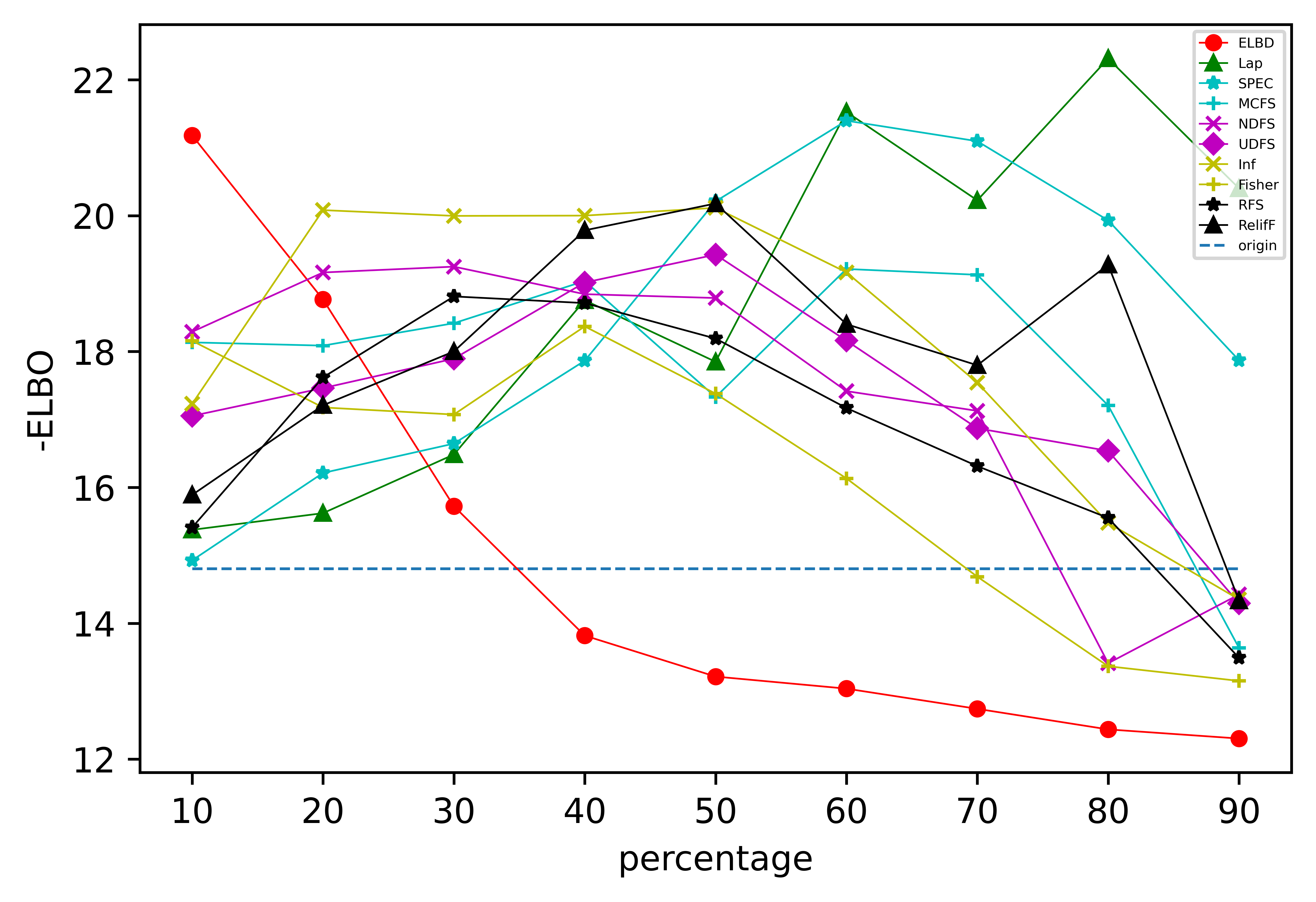
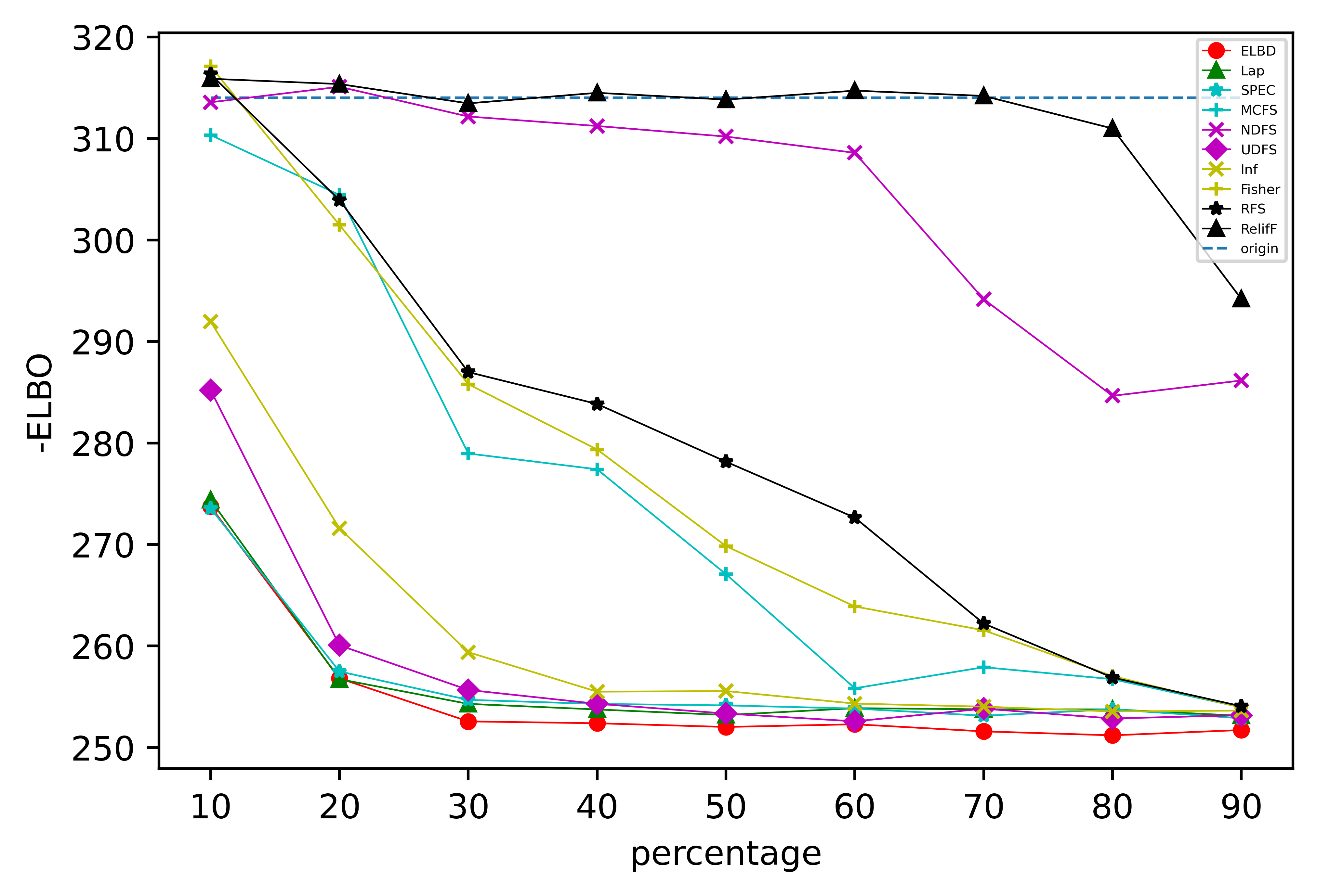
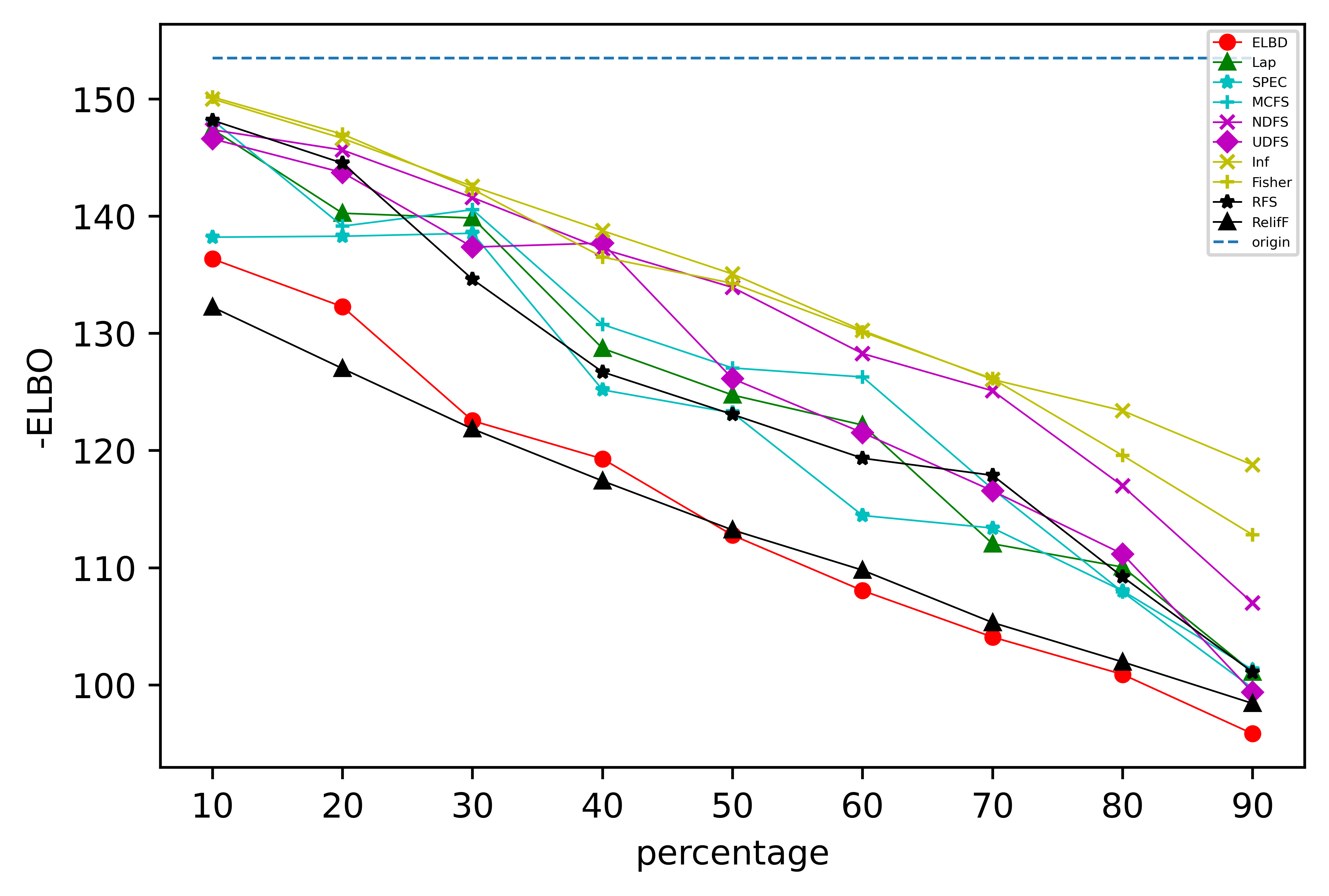
Constrained by the computational complexity, we only pick $60\%$ of latent variables to optimize models. However, we pick six different models to study the impact of the percentage on optimized result. The studies are shown in Figure 4. In each graph of Figure 4, the y axis represents -ELBO loss and x axis represents the percentage of latent variables we take by all feature selection algorithms from $10\%$ to $90\%$ (we can not pick $100\%$ since all the analyses in Section 3 are based on the assumption that $\dim\mathbf{w}>0$ and $\dim\mathbf{u}>0$). We find that for ELBD, in most of graphs, losses decrease with increasing of percentage of selected latent variables, and become stable or unchanged after certain percentage. It means the latent variable which has low ELBD score basically have no contribution on optimization. But for other feature selection algorithms, things become different. For example, models optimized by Inf in graph (b) and Lap in (d) become worse with increasing of percentage. We also find some algorithms can not optimize models. Therefore, not all the latent variables are worth being chosen as $\mathbf{u}$ and taking too much “bad” latent variables can increase the loss. However in graph (f), all the algorithms show strictly decreasing lines, we can draw the conclusion that all the latent variables in this latent variables of model are “good”.

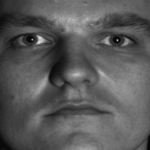
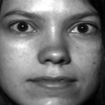
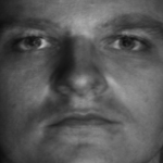
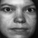
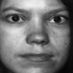
In Figure 5, we also show the original pictures on test set of Yale, pictures generated by model and pictures generated by optimized model. We may find that model after optimization generates more clear pictures.

5.2 gELBD Score on Classification task

In this subsection, we compare gELBD score with other 9 feature selection algorithms on classification tasks. We use full connect neural network to train the classification models. We use cross entropy as loss function in training step and use Adam algorithm to minimize the loss function. The learning rate is in $[1\times 10^{-3},1\times 10^{-4}]$.

As we mentioned at the end of Section 4, we need to discretize the features before applying gELBD. We multiply 255 and round-down to the closest integer on each feature. Then the value of every feature becomes the integer in $[0,255]$.

We still pick $60\%$ of features and use these features to train models. After getting selected features, we train five different models with different random seeds. The mean and standard deviation of accuracy $\frac{R}{N}$ is shown in Table X where $R$ is the number of instances which are classified correctly and $N$ is size of data set.

We can find that gELBD has the highest accuracy in these five data sets compare to other feature selection algorithms.

6 Conclusion

This paper is motivated by the fact that eliminating latent variables in VAE can increase the ELBO. According to this fact, this paper proposes algorithms to marginalize the encoder and proposes the weak convergence approximation algorithms to approximate decoder after eliminating latent variables $\mathbf{u}$. We also do lots of theoretical analyses to guarantee the convergence. We find that the weak convergence approximation algorithms actually increase the weights of distribution $Q(\mathbf{u}|\mathbf{x})$. Therefore we need to select important latent variables and do the weak convergence approximation algorithms only on them. Then we analyze the necessity of selecting latent variables and present a new feature selection algorithm ELBD and generalize ELBD on classification tasks as gELBD. In experiments, we use two kinds of loss functions to measure the optimized result on test sets. We find that both weak convergence approximation algorithms and ELBD have the best performance. And gELBD also achieves the highest accuracy in classification tasks. Besides VAE, CVAE, NF-VAE, IAF-VAE, we can use our algorithms on other variants of VAE. In latter research, we aim to expand the weak convergence approximation algorithms on more variational inference models. The computational complexity is the fatal drawback of ELBD and gELBD. How to overcome this drawback also needs our exploration.

Yiran Dong received the B.S. degree in Mathematics and Applied Mathematics from Sichuan University, China, in 2020. He is currently studying towards the Ph.D. degree in operational research and cybernetics in Zhejiang University. His researches mainly focus on generative models, Bayesian network and causal inference.

Chuanhou Gao received the B.Sc. degree in Chemical Engineering from Zhejiang University of Technology, China, in 1998, and the Ph.D. degree in Operational Research and Cybernetics from Zhejiang University, China, in 2004. From June 2004 until May 2006, he was a Postdoctor in the Department of Control Science and Engineering at Zhejiang University. Since June 2006, he has joined the Department of Mathematics at Zhejiang University, where he is currently a full Professor. He was a visiting scholar at Carnegie Mellon University from Oct. 2011 to Oct. 2012. His research interests are in the areas of data-driven modeling, control and optimization, chemical reaction network theory and thermodynamic process control. He is an associate editor of IEEE Transactions on Automatic Control and of International Journal of Adaptive Control and Signal Processing.

References

- [1] D. P. Kingma and M. Welling, “Auto-encoding variational bayes,” arXiv preprint arXiv:1312.6114, 2013.
- [2] C. Doersch, “Tutorial on variational autoencoders,” arXiv preprint arXiv:1606.05908, 2016.
- [3] K. Sohn, H. Lee, and X. Yan, “Learning structured output representation using deep conditional generative models,” Advances in neural information processing systems, vol. 28, 2015.
- [4] A. Razavi, A. v. d. Oord, B. Poole, and O. Vinyals, “Preventing posterior collapse with delta-vaes,” arXiv preprint arXiv:1901.03416, 2019.
- [5] D. P. Kingma, T. Salimans, R. Jozefowicz, X. Chen, I. Sutskever, and M. Welling, “Improved variational inference with inverse autoregressive flow,” Advances in neural information processing systems, vol. 29, 2016.
- [6] A. Razavi, A. Van den Oord, and O. Vinyals, “Generating diverse high-fidelity images with vq-vae-2,” Advances in neural information processing systems, vol. 32, 2019.
- [7] X. Ma, C. Zhou, and E. Hovy, “Mae: Mutual posterior-divergence regularization for variational autoencoders,” arXiv preprint arXiv:1901.01498, 2019.
- [8] A. Vahdat and J. Kautz, “Nvae: A deep hierarchical variational autoencoder,” Advances in Neural Information Processing Systems, vol. 33, pp. 19 667–19 679, 2020.
- [9] B. Samanta, A. De, G. Jana, V. Gómez, P. K. Chattaraj, N. Ganguly, and M. Gomez-Rodriguez, “Nevae: A deep generative model for molecular graphs,” Journal of machine learning research. 2020 Apr; 21 (114): 1-33, 2020.
- [10] S. R. Bowman, L. Vilnis, O. Vinyals, A. M. Dai, R. Jozefowicz, and S. Bengio, “Generating sentences from a continuous space,” arXiv preprint arXiv:1511.06349, 2015.
- [11] S. Lombardo, J. Han, C. Schroers, and S. Mandt, “Deep generative video compression,” Advances in Neural Information Processing Systems, vol. 32, 2019.
- [12] T. White, “Sampling generative networks,” arXiv preprint arXiv:1609.04468, 2016.
- [13] J. Li, K. Cheng, S. Wang, F. Morstatter, R. P. Trevino, J. Tang, and H. Liu, “Feature selection: A data perspective,” ACM computing surveys (CSUR), vol. 50, no. 6, pp. 1–45, 2017.
- [14] V. Kumar and S. Minz, “Feature selection: a literature review,” SmartCR, vol. 4, no. 3, pp. 211–229, 2014.
- [15] T. Hastie, R. Tibshirani, J. H. Friedman, and J. H. Friedman, The elements of statistical learning: data mining, inference, and prediction. Springer, 2009, vol. 2.
- [16] M. Robnik-Šikonja and I. Kononenko, “Theoretical and empirical analysis of relieff and rrelieff,” Machine learning, vol. 53, no. 1, pp. 23–69, 2003.
- [17] D. Rezende and S. Mohamed, “Variational inference with normalizing flows,” in International conference on machine learning. PMLR, 2015, pp. 1530–1538.
- [18] D. P. Kingma, M. Welling et al., “An introduction to variational autoencoders,” Foundations and Trends® in Machine Learning, vol. 12, no. 4, pp. 307–392, 2019.
- [19] W. H. Greub, Linear algebra. Springer Science & Business Media, 2012, vol. 23.
- [20] P. Billingsley, Probability and measure. John Wiley & Sons, 2008.
- [21] E. J. McShane and T. A. Botts, Real analysis. Courier Corporation, 2013.
- [22] Géron and Aurélien, Hands-on machine learning with Scikit-Learn, Keras, and TensorFlow: Concepts, tools, and techniques to build intelligent systems. ” O’Reilly Media, Inc.”, 2019.
- [23] C. M. Bishop and N. M. Nasrabadi, Pattern recognition and machine learning. Springer, 2006, vol. 4, no. 4.
- [24] Y. LeCun, L. Bottou, Y. Bengio, and P. Haffner, “Gradient-based learning applied to document recognition.” 1998.
- [25] T. Clanuwat, M. Bober-Irizar, A. Kitamoto, A. Lamb, K. Yamamoto, and D. Ha. (2018) Deep learning for classical japanese literature.
- [26] R. Arya, “Gesture-controlled-opencv-calculator,” https://github.com/rishabh-arya/Gesture-controlled-opencv-calculator, 2021.
- [27] P. Viradiya, “Fingers,” https://www.kaggle.com/datasets/koryakinp/fingers, 2019.
- [28] P. Koryakin, “Brian tumor dataset,” https://www.kaggle.com/datasets/preetviradiya/brian-tumor-dataset, 2021.
- [29] A. Georghiades, P. Belhumeur, and D. Kriegman, “From few to many: illumination cone models for face recognition under variable lighting and pose,” IEEE Transactions on Pattern Analysis and Machine Intelligence, vol. 23, no. 6, pp. 643–660, 2001.
- [30] D. Kermany, K. Zhang, and M. Goldbaum, “Large dataset of labeled optical coherence tomography (oct) and chest x-ray images,” 2018.
- [31] Z. Zhao and H. Liu, “Spectral feature selection for supervised and unsupervised learning,” pp. 1151–1157, 2007.
- [32] D. Cai, C. Zhang, and X. He, “Unsupervised feature selection for multi-cluster data,” pp. 333–342, 2010.
- [33] Z. Li, Y. Yang, J. Liu, X. Zhou, and H. Lu, “Unsupervised feature selection using nonnegative spectral analysis,” in Proceedings of the AAAI conference on artificial intelligence, vol. 26, no. 1, 2012, pp. 1026–1032.
- [34] Y. Yang, H. T. Shen, Z. Ma, Z. Huang, and X. Zhou, “L2, 1-norm regularized discriminative feature selection for unsupervised,” in Twenty-second international joint conference on artificial intelligence, 2011.
- [35] G. Roffo, S. Melzi, U. Castellani, A. Vinciarelli, and M. Cristani, “Infinite feature selection: A graph-based feature filtering approach,” IEEE Transactions on Pattern Analysis and Machine Intelligence, vol. 43, no. 12, pp. 4396–4410, 2021.
- [36] P. E. Hart, D. G. Stork, and R. O. Duda, Pattern classification. Wiley Hoboken, 2000.
- [37] F. Nie, H. Huang, X. Cai, and C. Ding, “Efficient and robust feature selection via joint l2, 1-norms minimization,” Advances in neural information processing systems, vol. 23, 2010.
- [38] H. Xiao, K. Rasul, and R. Vollgraf, “Fashion-mnist: a novel image dataset for benchmarking machine learning algorithms,” arXiv preprint arXiv:1708.07747, 2017.
- [39] G. Cohen, S. Afshar, J. Tapson, and A. Van Schaik, “Emnist: Extending mnist to handwritten letters,” in 2017 international joint conference on neural networks (IJCNN). IEEE, 2017, pp. 2921–2926.
- [40] F. Robert, “Hand-drawn shapes (hds) dataset,” https://github.com/frobertpixto/hand-drawn-shapes-dataset, 2022.
- [41] PavelBiz, “Chinese calligraphy styles by calligraphers,” https://www.kaggle.com/datasets/yuanhaowang486/chinese-calligraphy-styles-by-calligraphers, 2021.
- [42] Y. Wang, “Female and male eyes,” https://www.kaggle.com/datasets/pavelbiz/eyes-rtte, 2021.
- [43] D. P. Kingma and J. Ba, “Adam: A method for stochastic optimization,” arXiv preprint arXiv:1412.6980, 2014.
![[Uncaptioned image]](/html/2111.08493/assets/dyr.jpg)