Global dynamics of the Hořava-Lifshitz cosmology in the presence of non-zero cosmological constant in a flat space

Abstract.

Using the qualitative theory of differential equations, the global dynamics of a cosmological model based on Hořava-Lifshitz gravity is studied in the space with zero curvature in the presence of the non-zero cosmological constant.

1. Introduction

A decade ago Hořava [1] brought forward a new theory on space-time asymmetric gravitation, called Hořava-Lifshitz gravity, together with the scalar field theory of Lifshitz. This theory’s applications in cosmology, dark energy, and black hole have stimulated many studies (See review papers [20], [21] or regular literature [2]-[19]).

Based on whether the value of $\Lambda$ (cosmological constant) is zero and the flatness of the universe, i.e. whether the space curvature $k$ is equal to zero, Leon et al. [8, 9, 10, 16] divided Hořava-Lifshitz cosmology into four cases: (1) $\Lambda=0,k=0$; (2) $\Lambda=0,k\neq 0$; (3) $\Lambda\neq 0,k=0$; (4) $\Lambda\neq 0,k\neq 0$ under the classic FLRW metric. They either studied partially the three-dimensional dynamics of Hořava-Lifshitz cosmology, or analyzed its two-dimensional dynamics under the usual exponential potentials.

For the cosmological constant $\Lambda$ that scientists have been concerning about, Carlip [22] believed that the vacuum fluctuations under the standard effective field theory produce a huge $\Lambda$ and produce high $k$ on the Planck scale, but it is almost invisible at the observable scale. Compared with the prediction in the standard $\Lambda$ cold dark matter model, Valentino et al. [23] proposed that the cosmological space may be a closed three-dimensional sphere, i.e., the cosmological space’s curvature may be positive, based on the enhanced lensing amplitude in the cosmic microwave background power spectra confirmed by Planck Legacy 2018 release. Although this study provides the latest results, the debate about the universe’s shape has not yet been settled. An important reason is that the calculation of the critical density of the universe depends on the measurement of the Hubble constant, but it seems that this constant is still not accurate, then the boundary line of the universe is fuzzy, so it is too early to say that the universe must be closed.

The global dynamics of the Hořava-Lifshitz cosmology under the background of FLRW with $k=0,\Lambda=0$ was studied in [5], and the case of $k\neq 0,\Lambda=0$ has also been addressed in [6]. In this paper we will consider the flat universe with $\Lambda\neq 0$, the corresponding autonomous cosmological equations admit the following form

(1) $$\begin{array}[]{rl}\vspace{2mm}\dfrac{dx}{dt}&=\sqrt{6}s\left(z^{2}-x^{2}+1\right)+3x\left(x^{2}-1\right),\\ \vspace{2mm}\dfrac{dz}{dt}&=3zx^{2},\\ \vspace{2mm}\dfrac{ds}{dt}&=\dfrac{\sqrt{6}}{n}xs^{2}.\end{array}$$

The details for obtaining the cosmological equations (1) will be provided in Section 2.

2. The cosmological equations

In order to describe the cosmological model, we first briefly review the Hořava-Lifshitz theory of gravity proposed in [1]. The field content in this theory can be derived from the space vector $N_{i}$ and scalar $N$, see [10, 11]. They are actually common ‘lapse’ and ‘shift’ variables in general relativity. From this the complete metric can be expressed as

(2) $$\begin{array}[]{rl}ds^{2}=-N^{2}dt^{2}+g_{ij}(dx^{i}+N^{i}dt)(dx^{j}+N^{j}dt),\ \ \ N_{i}=g_{ij}N^{j},\end{array}$$

where $g_{ij}$ is a spatial metric, here $i$ and $j$ are natural numbers from 1 to 3. The coordinate transformations follow $t\to l^{3}t,\ x^{i}\to lx^{i}$. Note that $g_{ij}$ is invariant, the same as $N$, but $N^{i}$ is scaled to $l^{-2}N_{i}$.
According to the detailed-balance condition, the full gravitational action of Hořava-Lifshitz is expressed as

(3) $$\begin{array}[]{rl}\vspace{2mm}S_{g}=&\displaystyle\int dtd^{3}x\sqrt{g}N\left\{\dfrac{2}{\kappa^{2}}\left(K_{ij}K^{ij}-\lambda K^{2}\right)-\dfrac{\kappa^{2}}{2w^{4}}C_{ij}C^{ij}\right.\\ \vspace{2mm}\hfil&\ \ \ +\dfrac{\mu\kappa^{2}}{2w^{2}}\dfrac{\epsilon^{ijm}}{\sqrt{g}}R_{il}\nabla_{j}R^{l}_{k}-\dfrac{\mu^{2}\kappa^{2}}{8}R_{ij}R^{ij}\\ &\ \ \ -\left.\dfrac{\mu^{2}\kappa^{2}}{8(3\lambda-1)}\left(\dfrac{1-4\lambda}{4}R^{2}+\Lambda R-3\Lambda^{2}\right)\right\},\end{array}$$

where $C^{ij}=\epsilon^{ijm}\nabla_{k}\left(4R^{j}_{i}-R\delta^{j}_{i}\right)/(4\sqrt{g})$ denotes the Cotton tensor, $K_{ij}=(\dot{g}_{ij}-\nabla_{i}N_{j}-\nabla_{j}N_{i})/(2N)$ represents the extrinsic curvature, and $\epsilon^{ijm}/\sqrt{g}$ is the standard general covariant antisymmetric tensor, the indices are to up and down with the metric $g_{ij}$. $\kappa$, $\lambda$, $w$ and $\mu$ are all constants, for more details see [1].

Consider the gravitational action term on the potential $V(\phi)$ as follows

(4) $$\begin{array}[]{rl}\vspace{2mm}S=\displaystyle\int dtd^{3}x\sqrt{g}N\left(\dfrac{3\lambda-1}{4}\dfrac{\dot{\phi}^{2}}{N^{2}}-V(\phi)\right),\end{array}$$

and the metric $N^{i}=0$, $g_{ij}=a^{2}(t)\gamma_{ij}$, $\gamma_{ij}dx^{i}dx^{j}=r^{2}d\Omega^{2}_{2}+dr^{2}/(1-kr^{2})$. Above $a(t)$ represents the scale factor of the expanding universe, which is dimensionless, and $\gamma_{ij}$ refers to the constant curvature metric with maximally symmetric. For the flat space we take $k=0$ in this paper.
For the sake of simplicity, $\kappa^{2}$ and $N$ are normalized, and then the corresponding cosmological model can be interpreted as

(5) $$\begin{array}[]{rl}\vspace{2mm}\hfil&H^{2}=\dfrac{\dot{\phi}^{2}}{24}+\dfrac{V(\phi)}{6(3\lambda-1)}-\dfrac{\mu^{2}\Lambda^{2}}{16(3\lambda-1)^{2}},\\ \vspace{2mm}\hfil&\dot{H}+\dfrac{3}{2}H^{2}=-\dfrac{\dot{\phi}^{2}}{16}+\dfrac{V(\phi)}{4(3\lambda-1)}-\dfrac{3\mu^{2}\Lambda^{2}}{32(3\lambda-1)^{2}},\\ \vspace{2mm}\hfil&\ddot{\phi}+3H\dot{\phi}+\dfrac{2V^{\prime}(\phi)}{3\lambda-1}=0,\end{array}$$

where $H$ is the Hubble parameter and has the form $\dot{a}(t)/a(t)$.
Considering that $V(\phi)$ admits various mathematical forms (see [9, 24, 25, 26]), we just take $V(\phi)=(\mu\phi)^{2n}/2n$ with a natural number $n$ and a constant $\mu>0$ in this paper. Following [9, 10] we do the dimensionless transformation

(6) $$\begin{array}[]{rl}\vspace{2mm}\hfil&x=\dfrac{\dot{\phi}}{2\sqrt{6}H},\ \ \ y=\dfrac{\sqrt{V(\phi)}}{\sqrt{6}H\sqrt{3\lambda-1}},\ \ \ z=\dfrac{\Lambda\mu}{4(3\lambda-1)H},\\ \vspace{2mm}\hfil&s=-\dfrac{V^{\prime}(\phi)}{V(\phi)},\ \ \ f(s)\equiv\dfrac{V^{\prime\prime}(\phi)}{V(\phi)}-\dfrac{V^{\prime}(\phi)^{2}}{V(\phi)^{2}}.\end{array}$$

Thus we obtain $f(s)=-s^{2}/(2n)$, which is a power-law potential, so $ds/dt=\sqrt{6}xs^{2}/n$. Furthermore it can be followed from equations (5) and (6) that

(7) $$\begin{array}[]{rl}\vspace{2mm}x^{2}+y^{2}-z^{2}=1,\\ \vspace{2mm}\dfrac{H^{\prime}}{H}=-3x^{2}.\end{array}$$

Therefore the field equations become the dimensionless form provided in [1]. For more details on system (1) see the equations (205)-(207) of [9] or equations (52)-(54) of [16].

The present paper gives a fully description of the global dynamics of system (1) in the physical area of interest $G=\left\{(x,z,s)\in\mathbb{R}^{3}:x^{2}-z^{2}\leq 1\right\}$. In sections 3 and 4 we will investigate the phase portraits of system (1) at finite and infinite equilibrium points on invariant planes and surface. In section 5 we will discuss the phase portraits of system (1) inside the Poincaré ball restricted to the region $G$. An introduction to the Poincaré ball that can be used to study the dynamics of the system (1) near infinity can be found in the appendix. Based on these sections, considering the symmetry of system (1), we will study the global dynamics of system (1) adding its behavior at infinity in section 6. Moreover we will give the final discussion and summary in the last section 7.

3. Phase portraits on two invariant planes $z=0,\ s=0$ and on the invariant surface $x^{2}-z^{2}=1$

In order to clarify the local phase portraits of equilibrium points (finite and infinite) and the global phase portraits of system (1) in the aforementioned region $G$ (refer to [9] or [16] again). We begin to describe the phase portraits on the invariant planes $z=0,\ s=0$ and on the invariant surface $x^{2}-z^{2}=1$.

3.1. The invariant plane $z=0$

On the plane $z=0$ system (1) reduces to

(8) $$\begin{array}[]{rl}\dfrac{dx}{dt}&=\left(x^{2}-1\right)\left(3x-\sqrt{6}s\right),\\ \vspace{2mm}\dfrac{ds}{dt}&=\dfrac{\sqrt{6}}{n}\,xs^{2}.\end{array}$$

The phase portrait of the above system in the strip $z=0$ and $x^{2}-z^{2}\leq 1$ has been presented in [5] (see Figure 1). System (8) contains a hyperbolic equilibrium point $e_{0}=(0,0)$ and two semi-hyperbolic equilibrium points $e_{1}=(1,0)$, $e_{2}=(-1,0)$, where $e_{0}$ is a saddle point, and the other two are saddle-nodes.

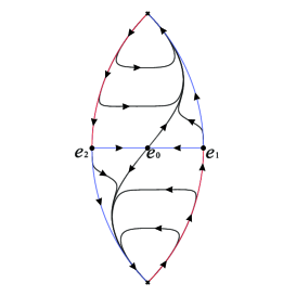
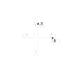
Figure 1. The phase portrait of system (1) on the invariant plane $z=0$ in the region $-1\leq x\leq 1$.

3.2. The invariant plane $s=0$

On the plane $s=0$ system (1) reduces

(9) $$\begin{array}[]{rl}\dfrac{dx}{dt}=3x\left(x^{2}-1\right),\ \dfrac{dz}{dt}=3zx^{2}.\end{array}$$

Note that the straight line $x=0$ is filled of equilibrium points. Introducing the transformation with respect to time $d\tau_{1}=xdt$ yields

(10) $$\begin{array}[]{rl}\dfrac{dx}{d\tau_{1}}=3\left(x^{2}-1\right),\ \dfrac{dz}{d\tau_{1}}=3zx,\end{array}$$

which has two hyperbolic equilibrium points $e_{1}=(1,0)$ and $e_{2}=(-1,0)$. Here $e_{1}$ is an unstable node and has two eigenvalues 3 and 6, but $e_{2}$ is a stable node and has eigenvalues -3 and -6.

According to the Poincaré compactification method (see Chapter 5 of [27] for more details), system (9) on the local chart $U_{1}$ reduces to

(11) $$\begin{array}[]{rl}\dfrac{du}{dt}=3uv^{2},\ \dfrac{dv}{dt}=3v\left(v^{2}-1\right).\end{array}$$

Since all the points at infinity (i.e. at $v=0$) of system (11) are equilibrium points, we do the transformation of the time $d\tau_{2}=vdt$, and the system (11) becomes

(12) $$\begin{array}[]{rl}\dfrac{du}{d\tau_{2}}=3uv,\ \dfrac{dv}{d\tau_{2}}=v^{2}-1.\end{array}$$

However there is no equilibrium points in system (12).

System (9) on the local chart $U_{2}$ becomes

(13) $$\begin{array}[]{rl}\dfrac{du}{dt}=-3uv^{2},\ \dfrac{dv}{dt}=-3u^{2}v.\end{array}$$

Since this system’s linear term is always equal to zero, the corresponding topological index is known to be zero by the Poincaré-Hopf Theorem (for more details, see Theorem 6.30 in [27]). To study the local phase portrait of the equilibrium point (0,0) of system (13), we use the vertical blow-up techniques (see Ref. [28]), i.e., let $w=v/u$ then we have

(14) $$\begin{array}[]{rl}\dfrac{du}{dt}=-3u^{3}w^{2},\ \dfrac{dw}{dt}=3u^{2}w(w^{2}-1).\end{array}$$

Rescaling system (14)’s time $t$ by doing $d\tau_{3}=3u^{2}wdt$ yields

(15) $$\begin{array}[]{rl}\dfrac{du}{d\tau_{3}}=-uw,\ \dfrac{dw}{d\tau_{3}}=w^{2}-1.\end{array}$$

This system admits two equilibrium points $(0,-1)$ and $(0,1)$ on $u=0$. Both of these two points are hyperbolic unstable saddle points with eigenvalues of $-2,\ 1$ and $2,\ -1$, respectively. The local phase portrait around them is shown in Figure 2(a). Note the time rescaling between the above two systems, the local phase portrait of system (14) can be found in Figure 2(b). Additionally, all points on the axes $u=0$ and $w=0$ are singularities of system (14). Since $u>0$ and $w>0$ in the first quadrant I of Figure 2(b), then $v=uw$ will decrease as $u$ decreases, so the local phase portrait in the quadrant I of the $u$-$w$ coordinate system (corresponding to system (14)) can be equivalently converted to the portrait in the first quadrant of the $u$-$v$ coordinate system (corresponding to system (13)). Similarly the local phase portraits in the quadrants II, III and IV of the $u$-$w$ coordinate system can also be equivalently converted to these portraits in the third, second and fourth quadrants of the $u$-$v$ coordinate system, respectively. Therefore the local phase portrait of system (13) is displayed in Figure 2(c), and the corresponding local phase portrait at the origins of $U_{2}$ and the symmetrical $V_{2}$ in the invariant plane $s=0$ can be found in Figure 2(d).

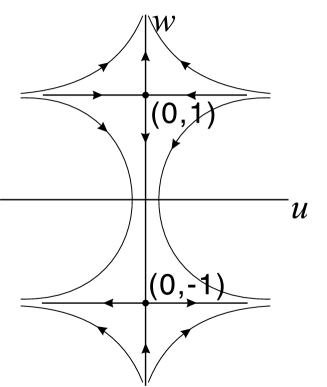
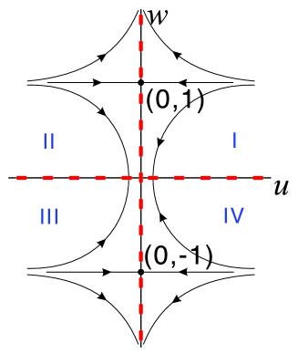
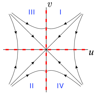
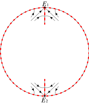
Figure 2. In (a), (b) and (c) there are the local phase portraits of the equilibrium points of systems (15), (14) and (13), respectively. In (d) there is the local phase portraits at the origins of $U_{2}$ and $V_{2}$ for $s=0$.

In summary, according to the previous information and considering that the straight lines $x=0$ and $z=0$ are invariant under the flow of system (9), we can obtain that in the Poincaré disk with $s=0$, the global phase portrait is restricted to the strip $-1\leq x\leq 1$ in Figure 3.

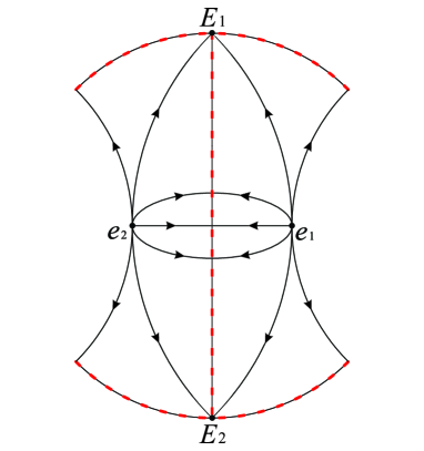
Figure 3. The phase portrait restricted to the region $x^{2}-z^{2}\leq 1$ on the invariant plane $s=0$ inside the Poincaré disc.

3.3. The invariant surface $x^{2}-z^{2}=1$

Under the flow of system (1), we first verify that $x^{2}-z^{2}=1$ is the invariant surface. If $l=l(x,z,s)=x^{2}-z^{2}-1$, then if the surface $x^{2}-z^{2}=1$ is invariant, then the polynomial $\mathcal{P}$ is required to make the equation

$$\frac{\partial l}{\partial x}\dot{x}+\frac{\partial l}{\partial z}\dot{z}+\frac{\partial l}{\partial s}\dot{s}=\mathcal{P}l,$$

true, which is exactly the case of $\mathcal{P}=2x(3x-\sqrt{6}s)$.

On the surface $x^{2}-z^{2}=1$ system (1) writes

(16) $$\begin{array}[]{rl}\dfrac{dx}{dt}=3x\left(x^{2}-1\right),\ \dfrac{ds}{dt}=\dfrac{\sqrt{6}}{n}\,xs^{2}.\end{array}$$

Then except for $s$-axis is filled with equilibrium points, the above system also has two finite semi-hyperbolic equilibrium points $e_{1}=(1,0)$ and $e_{2}=(-1,0)$. It can be followed from Theorem 2.19 of [27] that both $e_{1}$ and $e_{2}$ are saddle-nodes.

System (16) on the local chart $U_{1}$ writes

(17) $$\begin{array}[]{rl}\dfrac{du}{dt}=u\left[\dfrac{\sqrt{6}}{n}u+3\left(v^{2}-1\right)\right],\ \dfrac{dv}{dt}=3v\left(v^{2}-1\right).\end{array}$$

This system admits two infinite hyperbolic equilibrium points $e_{5}=(0,0)$ and $e_{6}=(\sqrt{6}n/2,0)$, where $e_{5}$ is a stable node and has eigenvalues $-3$ of multiplicity two, and the other point $e_{6}$ is an unstable saddle and has two eigenvalues $\pm 3$.

System (16) on the local chart $U_{2}$ can be written as

(18) $$\begin{array}[]{rl}\dfrac{du}{dt}=u\left[-\dfrac{\sqrt{6}}{n}u+3\left(u^{2}-v^{2}\right)\right],\ \dfrac{dv}{dt}=-\dfrac{\sqrt{6}}{n}\,uv.\end{array}$$

Rescaling the time $d\tau_{4}=udt$ we have

(19) $$\begin{array}[]{rl}\dfrac{du}{d\tau_{4}}=-\dfrac{\sqrt{6}}{n}u+3\left(u^{2}-v^{2}\right),\ \dfrac{dv}{d\tau_{4}}=-\dfrac{\sqrt{6}}{n}\,v.\end{array}$$

The origin $(0,0)$ of the above system is a hyperbolic stable node with eigenvalues $-\sqrt{6}/n$ and a multiplicity of 2. In this way, the origin $e_{7}=(0,0)$ of system (18) has a local phase portrait as shown in Figure 4.

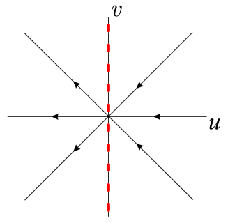
Figure 4. The local phase portrait at the origin of $U_{2}$ for $x^{2}-z^{2}=1$.

In summary the global phase portraits of system (16) is integrated in Figure 5.

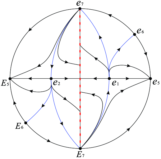
Figure 5. The phase portrait on the invariant surface $x^{2}-z^{2}=1$.

3.4. The finite equilibrium points

System (1) allows three three-dimensional finite equilibrium points $p_{0}=(0,0,0)$, $p_{1}=(1,0,0)$ and $p_{2}=(-1,0,0)$, $p_{0}$ has eigenvalues $-3,0,0$, $p_{1}$ and $p_{2}$ have the same eigenvalues $6,3,0$. Here $p_{1}$ and $p_{2}$ are the intersection points of $x^{2}-z^{2}=1$, $s=0$ and $z=0$ that were just studied in the previous subsections 3.1-3.3, that is, $p_{1}$ and $p_{2}$ are the equilibrium points $e_{1}$ and $e_{2}$, respectively. The origin $p_{0}$ is located in the middle of the intersection of $z=0$ and $s=0$, and it is the equilibrium point $e_{0}$ studied in the previous subsection 3.1.

4. Phase portrait on the surface of Poincaré ball at infinity

The three-dimensional Poincaré compactification (see Appendix or [29] for more details) is used to study the dynamics of the system (1) near infinity in this section. So we have $x=1/z_{3},\ z=z_{1}/z_{3},\ s=z_{2}/z_{3}$ on the local chart $U_{1}$, and then system (1) on the $U_{1}$ is reduced to

(20) $$\begin{array}[]{rl}\dfrac{dz_{1}}{dt}&=z_{1}\left[3z_{3}^{2}-\sqrt{6}z_{2}\left(-1+z_{1}^{2}+z_{3}^{2}\right)\right],\\ \dfrac{dz_{2}}{dt}&=z_{2}\left[3\left(z_{3}^{2}-1\right)+\sqrt{6}z_{2}\left(\dfrac{1+n}{n}-z_{1}^{2}-z_{3}^{2}\right)\right],\\ \dfrac{dz_{3}}{dt}&=z_{3}\left[3\left(z_{3}^{2}-1\right)+\sqrt{6}z_{2}\left(1-z_{1}^{2}-z_{3}^{2}\right)\right].\end{array}$$

In different local charts, $z_{3}=0$ corresponds to the infinity of $\mathbb{R}^{3}$. The equilibrium points of the system (20) are listed in Table 1, where the equilibrium point $u_{31}$ represents the origin of the local chart $U_{3}$, and the other equilibrium points lie in the local chart $U_{1}$. Additionally, for any constant $a$, $u_{a0}$ means that $s=0$ on local chart $U_{1}$ is filled with equilibrium points.

Table 1. The equilibrium points on the local charts of the surface of Poincaré ball at $\mathbb{R}^{3}$ infinity.

Equilibrium points	Eigenvalues
$u_{11}=(0,0,0)$	$-3,-3,0$
$u_{12}=\left(-1,\dfrac{\sqrt{6}}{2}n,0\right)$	$-3,3,-6n$
$u_{13}=\left(1,\dfrac{\sqrt{6}}{2}n,0\right)$	$-3,3,-6n$
$u_{14}=\left(0,\dfrac{\sqrt{6}n}{2(n+1)},0\right)$	$-\dfrac{3}{n+1},\dfrac{3n}{n+1},3$
$u_{a0}=(a,0,0)$	$-3,-3,0$
$u_{31}=(0,0,0)$	$0,0,0$

For the case $z_{3}=0$ system (20) becomes

(21) $$\begin{array}[]{rl}\dfrac{dz_{1}}{dt}&=\sqrt{6}z_{1}z_{2}\left(1-z_{1}^{2}\right),\\ \dfrac{dz_{2}}{dt}&=z_{2}\left[-3+\sqrt{6}z_{2}\left(\dfrac{1+n}{n}-z_{1}^{2}\right)\right].\end{array}$$

Rescaling the time $d\tau_{5}=z_{2}dt$, system (20) is reduced to

(22) $$\begin{array}[]{rl}\dfrac{dz_{1}}{d\tau_{5}}&=\sqrt{6}z_{1}\left(1-z_{1}^{2}\right),\\ \dfrac{dz_{2}}{d\tau_{5}}&=-3+\sqrt{6}z_{2}\left(\dfrac{1+n}{n}-z_{1}^{2}\right).\end{array}$$

Then system (22) allows equilibrium points $e_{i,1}$, $e_{i,2}$ and $e_{i,3}$, the coordinates of which are $(\mp 1,\sqrt{6}n/2)$ and $(0,\sqrt{6}n/(2n+2))$, respectively. The equilibrium points $e_{i,1}$ and $e_{i,2}$ are hyperbolic unstable saddles with eigenvalues $3$ and $-6n$, and the equilibrium point $e_{i,3}$ is a hyperbolic unstable node with eigenvalues $3n/(1+n)$ and $3$. The phase portrait on local chart $U_{1}$ of the Poincaré sphere at infinity is shown in Figure 6.

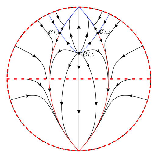
Figure 6. The phase portrait of system (1) on the local chart $U_{1}$ at infinity.

On the local chart $U_{2}$ we have Poincaré compactification $x=z_{1}/z_{3},\ z=1/z_{3},\ s=z_{2}/z_{3}$, the system (1) becomes

(23) $$\begin{array}[]{rl}\dfrac{dz_{1}}{dt}&=-z_{1}z_{3}^{2}+\sqrt{6}z_{2}\left(1-z_{1}^{2}+z_{3}^{2}\right),\\ \dfrac{dz_{2}}{dt}&=z_{1}z_{2}\left(-3z_{1}+\dfrac{\sqrt{6}}{n}z_{2}\right),\\ \dfrac{dz_{3}}{dt}&=-3z_{1}^{2}z_{3}.\end{array}$$

To study the phase portrait at infinity we take $z_{3}=0$, and changing the time $d\tau_{6}=z_{2}dt$ system (23) is equivalent to

(24) $$\begin{array}[]{rl}\dfrac{dz_{1}}{d\tau_{6}}&=\sqrt{6}\left(1-z_{1}^{2}\right),\\ \dfrac{dz_{2}}{d\tau_{6}}&=z_{1}\left(-3z_{1}+\dfrac{\sqrt{6}}{n}z_{2}\right).\end{array}$$

Since $(0,0)$ is the non-equilibrium point of system (24), there is no need to continue to investigate the equilibrium points at infinity in $U_{2}$. These have been discussed in the chart $U_{1}$.

On the local chart $U_{3}$ we have Poincaré compactification $x=z_{1}/z_{3},\ z=z_{2}/z_{3},\ s=1/z_{3}$, then system (1) writes

(25) $$\begin{array}[]{rl}\dfrac{dz_{1}}{dt}&=z_{1}\left[-\dfrac{\sqrt{6}(1+n)}{n}z_{1}+3z_{1}^{2}-3z_{3}^{2}\right]+\sqrt{6}\left(z_{2}^{2}+z_{3}^{2}\right),\\ \dfrac{dz_{2}}{dt}&=z_{1}z_{2}\left(-\dfrac{\sqrt{6}}{n}+3z_{1}\right),\\ \dfrac{dz_{3}}{dt}&=-\dfrac{\sqrt{6}}{n}z_{1}z_{3}.\end{array}$$

For the case $z_{3}=0$ it can be followed from system (25) that

(26) $$\begin{array}[]{rl}\dfrac{dz_{1}}{dt}&=z_{1}\left[-\dfrac{\sqrt{6}(1+n)}{n}z_{1}+3z_{1}^{2}\right]+\sqrt{6}z_{2}^{2},\\ \dfrac{dz_{2}}{dt}&=z_{1}z_{2}\left(-\dfrac{\sqrt{6}}{n}+3z_{1}\right).\end{array}$$

Note that the origin $(0,0)$ is a linearly zero equilibrium point of the above system. According to the Poincaré-Hopf Theorem, the topological index is zero. The vertical blow-up technique will be applied to investigate its local phase portrait. Then doing $w=z_{2}/z_{1}$ we have

(27) $$\begin{array}[]{rl}\dfrac{dz_{1}}{dt}&=z_{1}^{2}\left[\sqrt{6}\left(-\dfrac{1+n}{n}+w^{2}\right)+3z_{1}\right],\\ \dfrac{dw}{dt}&=\sqrt{6}z_{1}w\left(w^{2}-1\right).\end{array}$$

Rescaling the time $d\tau_{7}=z_{1}dt$ and eliminating the common factor $z_{1}$ of system (27), then we obtain

(28) $$\begin{array}[]{rl}\dfrac{dz_{1}}{d\tau_{7}}&=z_{1}\left[\sqrt{6}\left(-\dfrac{1+n}{n}+w^{2}\right)+3z_{1}\right],\\ \dfrac{dw}{d\tau_{7}}&=\sqrt{6}w\left(w^{2}-1\right).\end{array}$$

Since there are three hyperbolic equilibrium points $e_{i,4}=(0,-1)$, $e_{i,5}=(0,1)$ and $e_{i,6}=(0,0)$ of system (28) on $z_{1}=0$, the previous two are stable nodes with eigenvalues of $-2\sqrt{6}$ and $-\sqrt{6}/n$, the last one is an unstable saddle point with eigenvalues of $-\sqrt{6}(n+1)/n$ and $\sqrt{6}$. We note that this is the same as the equilibrium points in the system (26) of reference [6], so the local phase portraits of systems (28), (27) and (26) are shown in Figures 7(a), 7(b) and 7(c), respectively. Thus Figure 8 shows the phase portrait at the origin of the local chart $U_{3}$.

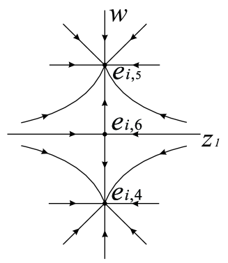
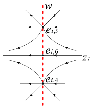
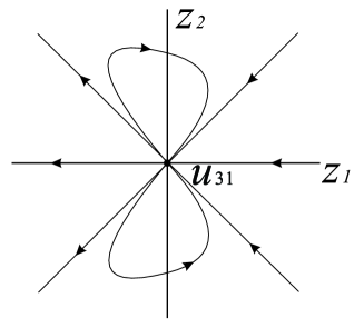
Figure 7. The local phase portraits (a), (b) and (c) of the above equilibrium points correspond to systems (28), (27) and (26) respectively.

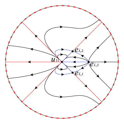
Figure 8. The phase portrait of system (1) in the local chart $U_{3}$ at infinity.

Combined with the previous discussion, Figure 9 shows the global phase portrait at infinity on the Poincaré sphere.

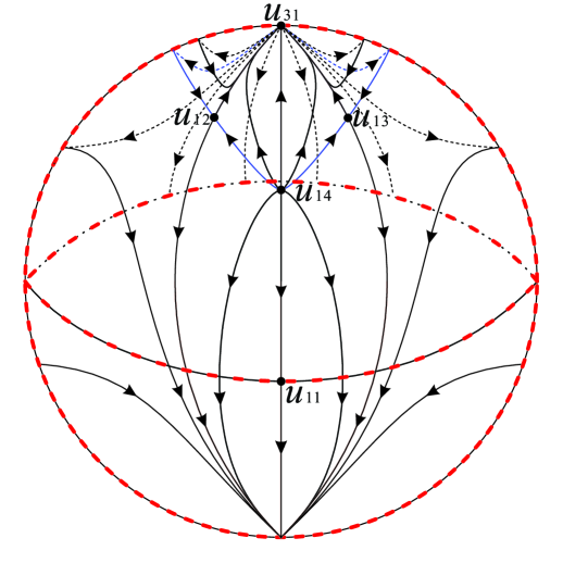
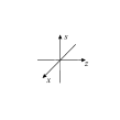
Figure 9. The global phase portrait of system (1) on the Poincaré sphere at infinity.

5. Phase portraits within the Poincaré sphere conditioned to $x^{2}-z^{2}\leq 1$

Since system (1) is invariant under the two symmetry about the origin and the $z$-axis, i.e., $(x,z,s)\mapsto(-x,-z,-s)$ and $(x,z,s)\mapsto(-x,z,-s)$. So we divide the Poincaré ball restricted to the region $G$ into four regions as follows

$$\begin{array}[]{rl}R_{1}:\ z\leq 0,\ s\geq 0.\ \ \ R_{3}:\ z\geq 0,\ s\geq 0.\\ R_{2}:\ z\leq 0,\ s\leq 0.\ \ \ R_{4}:\ z\geq 0,\ s\leq 0.\end{array}$$

In view of the aforementioned symmetries, we only need to focus on the phase portrait of system (1) in one region (such as $R_{1}$).

Combining the phase portrait in the invariant planes $s=0$, and $z=0$ with the phase portrait in the invariant surface $x^{2}-z^{2}=1$, and the phase portrait at infinity, the phase portrait on the boundary surface of $R_{1}$ is obtained in Figures 10-12.

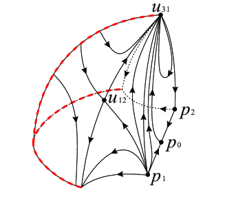
Figure 10. Phase portrait on the front boundary surface of $R_{1}$.

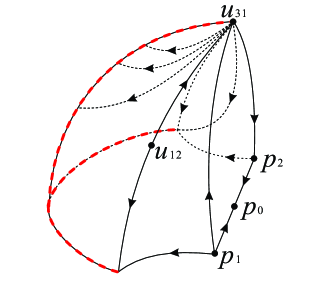
Figure 11. Phase portrait on the back boundary surface of $R_{1}$.

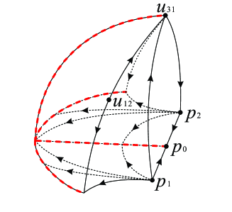
Figure 12. Phase portrait in the bottom plane of $R_{1}$.

Now we divide the boundary surface of the region $R_{1}$ into six parts (see Figure 13 for more details), thus the phase portrait of $R_{1}$ will be shown more clearly. It can be found from Figures 10 and 11 that the equilibrium point $u_{31}$ of the Poincaré ball is stable on the front boundary surfaces $F_{1}$ and $F_{2}$, and there is a stable parabolic sector and an elliptic sector segment $F_{3}$. However, on the back boundary surfaces $B_{1}$ and $B_{2}$, the north pole $u_{31}$ is unstable.

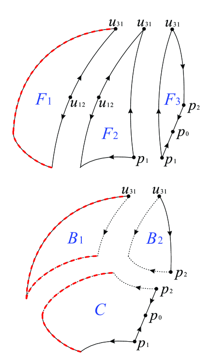
Figure 13. The six boundaries of $R_{1}$.

6. Dynamics inside the region $R_{1}$

System (1) has three finite equilibrium points $p_{0}$, $p_{1}$ and $p_{2}$. The dynamical behavior of system (1) in the Interior of the region $R_{1}$ depends on the comprehensive performance of the flow in the surface and planes

$$h(x,z,s)=0,\ x=0,\ z=0,\ s=0,$$

where

$$\begin{array}[]{rl}h(x,z,s)&=\sqrt{6}s\left(z^{2}-x^{2}+1\right)+3x\left(x^{2}-1\right).\end{array}$$

The above planes and surface cut the region $R_{1}$ into four different subregions $S_{i},\ i=(1,\dots,4)$, see Figures 14 and 15 for more details. It is noted that $h<0$ in the subregions $S_{1}$ and $S_{4}$, and $h>0$ in the subregions $S_{2}$ and $S_{3}$. To avoid confusion, please note that the solid and dotted lines in Figure 15 is consistent with those in Figure 14.

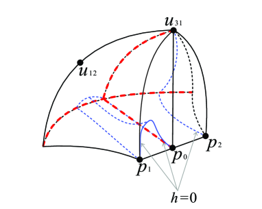
Figure 14. There are four subregions inside the region $R_{1}$ of the Poincaré ball.

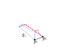
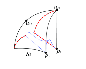
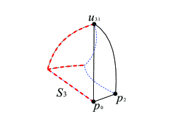
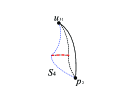
Figure 15. The four subregions $S_{i}$ of $R_{1}\ (i=1\cdots,4)$.

As it is shown in $S_{1}$ (see Figure 15(a)) the upper surface is included in the blue surface $h=0$, and the bottom plane is included in the invariant plane $s=0$. According to Table 2, the orbits monotonically decrease in the $x$ and $z$ directions. In the $s$ direction, they monotonically increase, so the orbits in the subregion $S_{1}$ can only start at the finite equilibrium point $p_{1}$ and pass through the upper surface of $S_{1}$ into the subregion $S_{2}$. However in subregion $S_{2}$ (see Figure 15(b), i.e. the remaining part after $S_{1}$ is extracted from the region $R_{1}$ when $x>0$), the orbits monotonically increase in the $x$ and $s$ directions but monotonically decrease in the $z$-direction, so we find that the orbits in $S_{2}$ can only start at $p_{1}$ or the equilibrium points on the negative $z$-axis, and they eventually towards the infinity equilibrium point $u_{12}$ fixed on the surface of $S_{2}$. Therefore the dynamic behavior of the orbits on these two subregions can be represented in the following form

Table 2. The dynamics of the four subregions.

Subregions	Associated Region	Monotonicity
$S_{1}$	$h<0,\ x>0,\ z<0,\ s>0$	$\dot{x}<0,\ \dot{z}<0,\ \dot{s}>0$
$S_{2}$	$h>0,\ x>0,\ z<0,\ s>0$	$\dot{x}>0,\ \dot{z}<0,\ \dot{s}>0$
$S_{3}$	$h>0,\ x<0,\ z<0,\ s>0$	$\dot{x}>0,\ \dot{z}<0,\ \dot{s}<0$
$S_{4}$	$h<0,\ x<0,\ z<0,\ s>0$	$\dot{x}<0,\ \dot{z}<0,\ \dot{s}<0$

In subregion $S_{3}$ (see Figure 15(c)) the left vertical plane facing us is contained in the plane $x=0$, and the right vertical plane is contained in the invariant plane $z=0$. In the opposite surfaces the left one is included in the surface of the Poincaré sphere, and the right one is included in the surface $h=0$. Since the orbits in $S_{3}$ monotonically decrease in the $z$ and $s$ directions, and they increase monotonically in the $x$ direction, it follows that the orbits will eventually go to the equilibrium point which lie in the equator or go to the negative $z$-axis in that region, and the orbits in this region may only come from the adjacent subregion $S_{4}$ (see Figure 15(d)). The left and right surfaces of subregion $S_{4}$ belong to the surfaces $h=0$ and $x^{2}-z^{2}=1\ (x<0)$, respectively. Since all the orbits are monotonically decreasing in $S_{4}$, the orbits in this region arrive from the infinite equilibrium point $u_{31}$, i.e. north pole of the Poincaré ball, and tend to the infinite equilibrium points on the equator of this region at a future date, or enter into the subregion $S_{3}$. This dynamical behavior can be represented as follows

Therefore the orbits’ dynamic behavior inside the four subregions of $R_{1}$ investigated above can be condensed to

This flow chart states clearly that the orbits of system (1) included in $R_{1}$ have $\alpha$-limit at $p_{1}$ and the north pole $u_{31}$ (also referred to as past attractors or negative attractors) of the Poincaré sphere. Additionally the orbits have $\omega$-limit either at $u_{12}$ (also called future attractor or positive attractor), or other infinite equilibrium points on the equator of subregions $S_{3}$ and $S_{4}$, which are located at the intersection of the Poincaré ball and at the infinity of the invariant planes $s=0$ in $\mathbb{R}^{3}$ when $x<0$, see Figure 14 or Figures 15(c) and 15(d).

Therefore all the global dynamical behavior of the system (1) is represented qualitatively and completely.

7. Conclusions

In the present paper we have fully described the global phase portrait of Hořava-Lifshitz cosmology in the presence of non-zero cosmological constant and zero curvature in the region of physical interest $G$. By taking the fact that the cosmological equations remains invariant under the two symmetries mentioned in section 5, the global phase portrait of the cosmological model in $G$ is provided completely.

From the perspective of cosmology, combined with the previous analysis of the phase portraits of the system, we know that the unstable finite equilibrium points $p_{1}$ and $p_{2}$ are dominated by dark matter, and the finite equilibrium $p_{0}$ located on the equilibrium point line may also be characterized by dark matter if the initial conditions are not in the invariant plane $z=0$. Besides the initial conditions in the invariant planes $s=0$ and $z=0$ as well as on the backside of the invariant surface $x^{2}-z^{2}=1$, the phase portrait displays that the eventual evolution of the orbits of the cosmological model in $G$ tends to the infinite equilibrium point $u_{12}$, which can be the late-time state of the universe and to other infinite equilibrium points placed at the equator of the Poincaré ball. For the Hořava-Lifshitz gravity in a FLRW space-time with $k=0$ and $\Lambda\neq 0$, equations (6) implies that the Hubble parameter $H$ tends to nil in forward time in this cosmological model.

Appendix: The Poincaré compactification in $\mathbb{R}^{3}$

For a polynomial vector field $X$$=(P_{1},P_{2},P_{3})$, and the degree $n=\max{\{\deg(P_{i}):i=1,2,3\}}$, its differential system is

$$\begin{array}[]{rl}\dfrac{dx}{dt}=P_{1}(x,y,z),\ \dfrac{dy}{dt}=P_{2}(x,y,z),\ \dfrac{dz}{dt}=P_{3}(x,y,z).\end{array}$$

Defining the unit sphere in $\mathbb{R}^{4}$ by $\mathbb{S}^{3}={\{y=(y_{1},y_{2},y_{3},y_{4})\in\mathbb{R}^{4}:}$ ${\|y\|=1\}}$, we denote the northern hemisphere by $\mathbb{S}_{+}={\{y\in\mathbb{S}^{3}:}$ ${y_{4}>0\}}$, the southern hemisphere by $\mathbb{S}_{-}={\{y\in\mathbb{S}^{3}:}$ ${y_{4}<0\}}$, the equator of $\mathbb{S}^{3}$ by the sphere by $\mathbb{S}^{2}={\{y\in\mathbb{S}^{3}:y_{4}=0\}}$, the tangent space at the point $y$ of $\mathbb{S}^{3}$ by $T_{y}\mathbb{S}^{3}$. Hence the tangent hyperplane $T_{(0,0,0,1)}\mathbb{S}^{3}=$ ${\{(x_{1},x_{2},x_{3},1)}$ ${\in\mathbb{R}^{4}:(x_{1},x_{2},x_{3})\in\mathbb{R}^{3}\}}$ is identified with $\mathbb{R}^{3}$. Moreover let

$$\begin{array}[]{rl}f_{+}:\mathbb{R}^{3}=T_{(0,0,0,1)}\mathbb{S}^{3}\to\mathbb{S}+,\ \ \ f_{+}(x)=\dfrac{1}{\Delta x}(x_{1},x_{2},x_{3},1),\end{array}$$

and

$$\begin{array}[]{rl}f_{-}:\mathbb{R}^{3}=T_{(0,0,0,1)}\mathbb{S}^{3}\to\mathbb{S}-,\ \ \ f_{-}(x)=-\dfrac{1}{\Delta x}(x_{1},x_{2},x_{3},1),\end{array}$$

be the two central projections, where $\Delta x=\left(\sum^{3}_{i=1}x^{2}_{i}+1\right)^{1/2}$. Then $f_{+}$ and $f_{-}$ are identified by $\mathbb{R}^{3}$ with the two hemispheres of $\mathbb{S}^{3}$. These two central projections clarify two transcripts of $X$, i.e. $Df_{+}\circ X$ in $\mathbb{S}_{+}$, and $Df_{-}\circ X$ in $\mathbb{S}_{-}$. Let $\widetilde{X}$ be the vector field on $\mathbb{S}^{3}\backslash\mathbb{S}^{2}=\mathbb{S}_{+}\cup\mathbb{S}_{-}$.
Now we analytically continue the vector field $\widetilde{X}(y)$ to the entire sphere $\mathbb{S}^{3}$ by $p(X)(y)=y^{n-1}_{4}\widetilde{X}(y)$. The continued vector field $p(X)$ is named Poincaré compactification of $X$. We note that the infinity of $\mathbb{R}^{3}$ represented by $\mathbb{S}^{2}$ is invariant for the vector field $p(X)$. The compactification for polynomial vector fields in $\mathbb{R}^{2}$ was introduced by Poincaré, and one can find its extension to $\mathbb{R}^{m}$ from [29]. Next we shall study the orthogonal projection of the closed $\mathbb{S}_{+}$ to $y_{4}=0$, which is a closed ball $B$ (designated Poincaré ball) with radius 1, its inner area is diffeomorphic to $\mathbb{R}^{3}$, and its boundary surface $\mathbb{S}^{2}$ is identified with $\mathbb{R}^{3}$ at infinity.
Since $\mathbb{S}^{3}$ is a differentiable manifold, we must consider eight local charts $(U_{i},F_{i})$ and $(V_{i},G_{i})$ in order to study the dynamics of $p(X)$, where

$$\begin{array}[]{rl}U_{i}={\{y\in\mathbb{S}^{3}:y_{i}>0\}},\ \ \ V_{i}={\{y\in\mathbb{S}^{3}:y_{i}<0\}},\end{array}$$

and the diffeomorphisms

$$\begin{array}[]{rl}F_{i}:U_{i}\to\mathbb{R}^{3},\ \ \ G_{i}:V_{i}\to\mathbb{R}^{3}\ \ \ \text{for}\ i=1,2,3,4,\end{array}$$

are the central projections’ inverses from the origin to the center of the tangent planes at the points $(\pm 1,0,0,0)$, $(0,\pm 1,0,0)$, $(0,0,\pm 1,0)$ and $(0,0,0,\pm 1)$, respectively. Then the expression of $p(X)$ in the local chart $U_{1}$ is

$$\begin{array}[]{rl}\dfrac{z^{n}_{3}}{(\Delta z)^{n-1}}(-z_{1}P_{1}+P_{2},-z_{2}P_{1}+P_{3},-z_{3}P_{1}),\end{array}$$

where $P_{i}=P_{i}(1/z_{3},z_{1}/z_{3},z_{2}/z_{3})$. In the local chart $U_{2}$ we have

$$\begin{array}[]{rl}\dfrac{z^{n}_{3}}{(\Delta z)^{n-1}}(-z_{1}P_{2}+P_{1},-z_{2}P_{2}+P_{3},-z_{3}P_{2}),\end{array}$$

where $P_{i}=P_{i}(z_{1}/z_{3},1/z_{3},z_{2}/z_{3})$. In the local chart $U_{3}$ we obtain

$$\begin{array}[]{rl}\dfrac{z^{n}_{3}}{(\Delta z)^{n-1}}(-z_{1}P_{3}+P_{1},-z_{2}P_{3}+P_{2},-z_{3}P_{3}),\end{array}$$

where $P_{i}=P_{i}(z_{1}/z_{3},z_{2}/z_{3},1/z_{3})$. In the local chart $U_{4}$ we get

$$\begin{array}[]{rl}z_{3}^{n-1}(P_{1},P_{2},P_{3}),\end{array}$$

where $P_{i}=P_{i}(z_{1},z_{2},z_{3})$. Furthermore the demonstration of $p(X)$ in the local chart $V_{i}$ is the same as in the $U_{i}$ multiplied by $(-1)^{n-1}$.
In addition the above factor $1/(\Delta z)^{n-1}$ is omitted by doing a time rescaling when we use the expressions of the compactified vector field $p(X)$ in the local charts.

References

- [1] P. Hořava, Quantum gravity at a Lifshitz point, Physical Review D 79, 084008, 2009.
- [2] E.M.C. Abreu, A.C.R. Mendes, G. Oliveira-Neto et al., Hořava-Lifshitz cosmological models with noncommutative phase space variables, General Relativity and Gravitation 51, 95, 2019.
- [3] S. Carloni, E. Elizalde and P.J. Silva, An analysis of the phase space of Hořava-Lifshitz cosmologies. In: S.D. Odintsov, D. Sáez-Gómez and S. Xambó-Descamps (eds) Cosmology, Quantum Vacuum and Zeta Functions, Springer Proceedings in Physics 137, 139-148, Springer-Verlag, Berlin, 2011.
- [4] B. Chen, On Hořava-Lifshitz cosmology, Chinese Physics C 35(5), 429-435, 2011.
- [5] F.B. Gao and J. Llibre, Global dynamics of the Hořava-Lifshitz cosmological system, General Relativity and Gravitation 51, 152, 2019.
- [6] F.B. Gao and J. Llibre, Global dynamics of Hořava-Lifshitz cosmology with non-zero curvature and a wide range of potentials, The European Physical Journal C 80, 137, 2020.
- [7] X. Gao,Y. Wang, R. Brandenberger and A. Riotto, Cosmological perturbations in Hořava-Lifshitz gravity, Physical Review D 81, 083508, 2010.
- [8] G. Leon and C.R. Fadragas, Cosmological dynamical systems: and their applications, Lambert Academic Publishing, GmbH Co. KG, Saarbrcken, 2012.
- [9] G. Leon and A. Paliathanasis, Extended phase-space analysis of the Hořava-Lifshitz cosmology, The European Physical Journal C 79, 746, 2019.
- [10] G. Leon and E.N. Saridakis, Phase-space analysis of Hořava-Lifshitz cosmology, Journal of Cosmology and Astroparticle Physics 2009, 006, 2009.
- [11] E. Kiritsis and G. Kofinas, Hořava-Lifshitz cosmology, Nuclear Physics B 821, 467-480, 2009.
- [12] S. Lepe and J. Saavedra, On Hořava-Lifshitz cosmology, Astrophysics and Space Science 350, 839-843, 2014.
- [13] A. Sheykhi, S. Ghaffari and H. Moradpour, Ghost dark energy in the deformed Hořava-Lifshitz cosmology, International Journal of Modern Physics D 28(06), 1950080, 2019.
- [14] R. Cordero, H. García-Compeán and F.J. Turrubiates, A phase space description of the FLRW quantum cosmology in Hořava-Lifshitz type gravity, General Relativity and Gravitation 51, 138, 2019.
- [15] N.A. Nilsson and E. Czuchry, Hořava-Lifshitz cosmology in light of new data, Physics of the Dark Universe 23, 100253, 2019.
- [16] A. Paliathanasis and G. Leon, Cosmological solutions in Hořava-Lifshitz scalar field theory, Zeitschrift fr Naturforschung A 75(6), 523-532, 2020.
- [17] E.N. Saridakis, Aspects of Hořava-Lifshitz cosmology, International Journal of Modern Physics D 20(08), 1485-1504, 2011.
- [18] A. Tawfik and E. Abou El Dahab, FLRW cosmology with Hořava-Lifshitz gravity: impacts of equations of state, International Journal of Theoretical Physics 56(7), 2122-2139, 2017.
- [19] M. Bhattacharjee, Gravitational radiation and black hole formation from gravitational collapse in theories of gravity with broken Lorentz symmetry, Baylor University, ProQuest Dissertations Publishing 22585106, 2019.
- [20] S. Mukohyama, Hořava-Lifshitz cosmology: a review, Classical and Quantum Gravity 27, 223101, 2010.
- [21] T.P. Sotiriou, Hořava-Lifshitz gravity: a status report, Journal of Physics: Conference Series 283, 012034, 2011.
- [22] S. Carlip, Hiding the cosmological constant, Physical Review Letters 123, 131302, 2019.
- [23] E. Di Valentino, A. Melchiorri and J. Silk, Planck evidence for a closed universe and a possible crisis for cosmology, Nature Astronomy 4, 196-203, 2020.
- [24] C.R. Fadragas, G. Leon and E.N. Saridakis, Dynamical analysis of anisotropic scalar-field cosmologies for a wide range of potentials, Classical and Quantum Gravity 31, 075018, 2014.
- [25] D. Escobar, C.R. Fadragas, G. Leon and Y. Leyva, Asymptotic behavior of a scalar field with an arbitrary potential trapped on a Randall-Sundrum’s braneworld: the effect of a negative dark radiation term on a Bianchi I brane, Astrophysics and Space Science 349, 575-602, 2014.
- [26] A. Alho, J. Hell and C. Uggla, Global dynamics and asymptotics for monomial scalar field potentials and perfect fluids, Classical and Quantum Gravity 32, 145005, 2015.
- [27] F. Dumortier, J. Llibre and J.C. Artés, Qualitative theory of planar differential systems, Springer-Verlag, Berlin, 2006.
- [28] M.J. Álvarez, A. Ferragut and X. Jarque, A survey on the blow up technique, International Journal of Bifurcation and Chaos 21(11), 3103-3118, 2011.
- [29] A. Cima and J. Llibre, Bounded polynomial vector fields, Transactions of the American Mathematical Society 318(2), 557-579, 1990.