Image-specific Convolutional Kernel Modulation for
Single Image Super-resolution

Abstract

Recently, deep-learning-based super-resolution methods have achieved excellent performances, but mainly focus on training a single generalized deep network by feeding numerous samples. Yet intuitively, each image has its representation, and is expected to acquire an adaptive model. For this issue, we propose a novel image-specific convolutional kernel modulation (IKM) by exploiting the global contextual information of image or feature to generate an attention weight for adaptively modulating the convolutional kernels, which outperforms the vanilla convolution and several existing attention mechanisms while embedding into the state-of-the-art architectures without any additional parameters. Particularly, to optimize our IKM in mini-batch training, we introduce an image-specific optimization (IsO) algorithm, which is more effective than the conventional mini-batch SGD optimization. Furthermore, we investigate the effect of IKM on the state-of-the-art architectures and exploit a new backbone with U-style residual learning and hourglass dense block learning, terms U-Hourglass Dense Network (U-HDN), which is an appropriate architecture to utmost improve the effectiveness of IKM theoretically and experimentally. Extensive experiments on single image super-resolution show that the proposed methods achieve superior performances over state-of-the-art methods. Code is available at github.com/YuanfeiHuang/IKM.

I Introduction

Single image super-resolution (SR) aims at reconstructing a high-resolution (HR) image from a single low-resolution (LR) image obtained by limited imaging devices, which is considered as a challenging ill-posed inverse problem and widely used in computer vision applications where high-frequency details are greatly desired, such as medical imaging, security, and surveillance.

For decades, numerous methods have been proposed to solve this ill-posed problem. For example, the interpolation-based [1, 2], the reconstruction-based [3, 4], and the example-learning-based [5, 6, 7, 8, 9, 10] methods. Recently, with the development of high-profile graphic process units (GPUs) and large-scale visual datasets, convolutional neural network (CNN) has obtained continuous attention as a dominant machine learning method in a majority of computer vision applications [11, 12, 13, 14, 15, 16, 17]. Moreover, benefited from the excellent ability to end-to-end nonlinear mapping on paired images, deep-learning-based methods have been also exploited for pixel-wise image reconstruction in low-level vision.

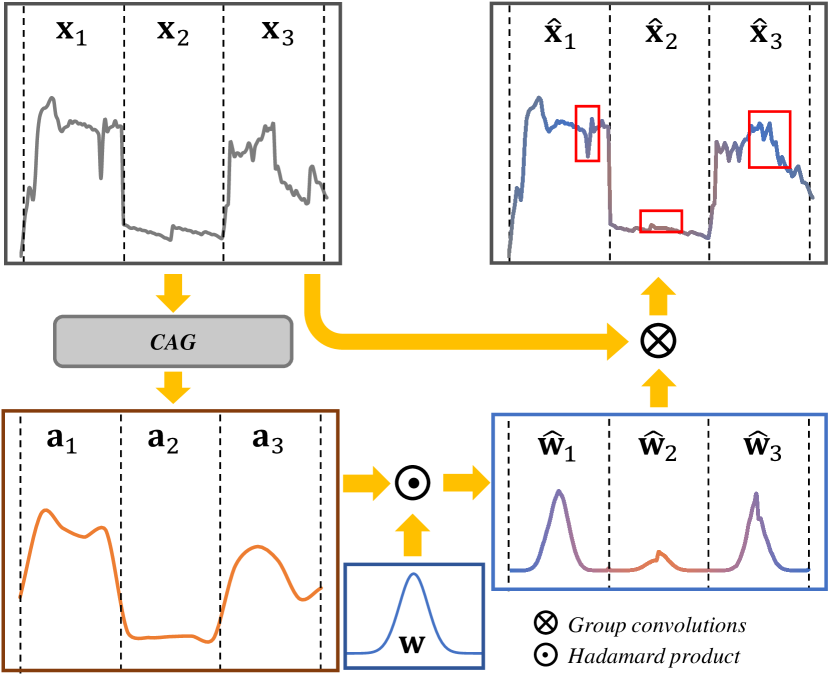
Figure 1: Illustration of IKM on 1D synthesized data. Particularly, features in each batch could be self-enhanced by adaptively applying the group convolutions with image-specific modulated kernel weights.

As the first attempt, Dong et al. [18, 19] proposed a shallow super-resolution convolutional neural network (SRCNN) by stacking several activated convolutional layers to learn the nonlinear mappings of LR-to-HR pairs, which outperforms most existing example-based SR methods and leads the trend of using end-to-end networks for SR. To facilitate the training of deep CNNs, Kim et al. further proposed the accurate VDSR [20] and firstly demonstrated the effectiveness of residual learning in end-to-end SR networks. However, training a very deep network is still hard as gradient vanishing/exploding, then local residual learning from ResNet [15] was arisen in SR [21, 22, 23] and achieved excellent performances. Besides, aiming at fully using the information flow of intermediate features in a network, densely connection [16] was also developed in SR [24, 25, 26, 27, 28]. Besides, to reduce the computational complexities, the transposed convolution (deconvolution) [29] and sub-pixel convolution [30] were proposed to upscale the images/features and limit the spatial size of LR input to speed up the inference. Moreover, the informativeness of features is also an important issue to improve the performance, then attention mechanism was highlighted, such as channel attention [17, 31], spatial attention [32, 33], non-local attention [34, 35], and task-specific attention [36]. Nevertheless, these methods mainly focus on training a single generalized deep network by feeding numerous samples, i.e., data-driven method.

Intuitively, each image has its representation, and then is expected to acquire an adaptive model. To implement this expectation, image-specific SR methods have been proposed by zero-shot learning [37, 38], but they are time-consuming as training an image-specific model from scratch. For a similar purpose but to be more efficient, we expect to bridge the gap between the data-driven and image-specific SR methods, and particularly make the following key contributions:

• We propose a novel image-specific convolutional kernel modulation (IKM) by exploiting the global contextual information of image/feature to generate an attention weight for adaptively modulating the convolutional kernels, which outperforms the vanilla convolution and other attention mechanisms when embedding into the state-of-the-art architectures without any additional parameters. An intuitive illustration of IKM on 1D synthesized data is shown in Fig. 1.

• We propose an image-specific optimization (IsO) algorithm for optimizing IKM in mini-batch training, which is a feasible algorithm to optimize the kernel weights and backward propagate the image-specific gradients, both of which positively guide the optimization on IKM.

• We design a new U-hourglass dense network (U-HDN) as the backbone to improve the capacity of model, by utilizing U-style residual leaning and hourglass dense block learning, which are demonstrated to be appropriate architectures for utmost improving the effectiveness of IKM theoretically and experimentally.

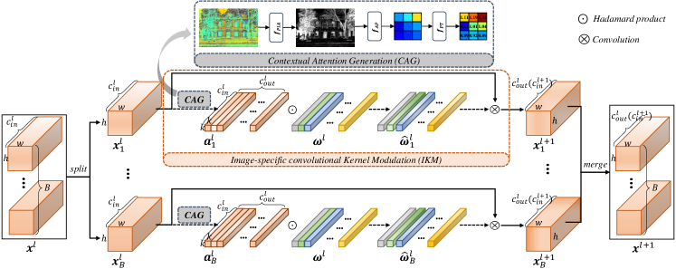
Figure 2: The pipeline of IKM. In $l$-th layer, $\{\boldsymbol{x}^{l}_{i}\}_{i=1}^{B}$ are firstly split in batch-wise into $B$ inputs, where each $\boldsymbol{x}^{l}_{i}$ is fed into a contextual attention generation module (CAG) to generate kernel attentions $\boldsymbol{a}_{i}^{l}$, and then self-enhanced in local receptive field with the modulated kernels ${\boldsymbol{\hat{w}}}_{i}^{l}$. And finally these enhanced features $\{{\boldsymbol{\hat{x}}}_{i}^{l}\}_{i=1}^{B}$ are merged into a mini-batch to next layer as $\{\boldsymbol{x}_{i}^{l+1}\}_{i=1}^{B}$.

II Related Work

Since the proposed IKM is implemented by generating an image-specific attention weight to modulate the convolutional kernels, we then describe several attention mechanisms and the deep-learning-based SR methods in this section.

II-A Attention Mechanisms

As the complexity of networks increases, the redundancy of learned features becomes an urgent issue. For efficiently exploiting a scalar response to represent the relative importance of components in feature, some recent researches have applied attention mechanism into the backbone architectures for image classification [17], image captioning [39, 40], low-level vision [31, 35, 33, 36], and etc. In particular, the implementation of attention mechanism can be divided into two branches: post hoc network analysis and trainable attention mechanism [42]. The post hoc network analysis [42, 43] is implemented by back-propagating the excited responses with respect to the high score target, with no need for additional learnable parameters. Moreover, as an end-to-end architecture, the trainable attention mechanism has been widely applied and developed by utilizing the forward feature maps to generate its spatial-attention or channel-attention weights through several additional non-linear transformations and further recalibrating the features in the corresponding locations or channels. Hu et al. proposed the squeeze-and-excitation networks (SENet) [17] to recalibrate the features with learnable channel-attention for improving the diversity of features, and has been extended into super-resolution, e.g., residual channel attention network (RCAN) [31]. In order to utilize the contextual spatial information in features, two-step attention mechanisms are then raised for gathering the spatial-wise enhancement and channel-wise recalibration, e.g., CBAM [32] and CSFM [33]. Furthermore, to enable the network to focus on the details, Huang et al. proposed the interpretable detail-fidelity attention network (DeFiAN) [36] by theoretically demonstrating the representative capacity of Hessian features.

II-B Deep-learning-based SR

Initially, SRCNN [19] was proposed to learn a nonlinear LR-to-HR mapping function as a high-capacity dictionary for sparse representation. To build deeper networks, Kim et al. further proposed the accurate VDSR [20] and firstly demonstrated the effectiveness of residual learning in end-to-end SR networks. Furthermore, SRResNet [21] was proposed by straightly stacking the post-activated residual blocks [15] to build a very deep backbone. However, specifically to single image super-resolution, batch normalization (BN) is undesired as weakening the diverse features, then EDSR [23] was proposed by removing all the BN operations in SRResNet and achieved excellent performances. Furthermore, inspired by DenseNet [16], dense connection was applied into SR tasks by densely integrating the information flow of intermediate features, e.g., SRDenseNet [24], MemNet [25], RDN [26, 27] and GLADSR [28].

However, as the depth and width of the network increase, higher computational complexity becomes a tough issue. Hence lightweight architectures are urgently needed for mobile applications with lower storage and lower computational capacities than the large cluster of GPUs. For example, aiming at reducing the space complexity for storage, DRCN [44] and DRRN [22] stacks deep convolution layers with weight sharing, which recursively calls a single block throughout the whole network. Meanwhile, to reduce the time complexity in model training and testing, lightweight architectures are designed using information diffluence, which splits the features and processes them separately in a manner of connection or convolution, e.g., IDN [45], MSRN [46], CARN [47] and MS³-Conv [48]. Moreover, to deal with this time-consuming issue, the transposed convolution (deconvolution) [29] and sub-pixel convolutions [30] were developed to upscale the features in the tail, and limit the spatial size of LR input to alleviate the time complexity. Furthermore, for larger upscaling factors (e.g., $\times 8$ upscaling), Laplacian pyramid networks were proposed for super-resolution by reconstructing the sub-band residual HR images at multiple pyramid levels [49, 50].

III Proposed Method

In this section, we first describe the motivation, inference, and optimization of IKM, and the conditions on utmost improving the performance of IKM. Under these conditions, we further describe the U-HDN architecture.

III-A Image-specific Convolutional Kernel Modulation

To improve the ability to non-linear representation, the existing state-of-the-art SR methods tend to build deeper or wider architectures. Particularly, by adaptively enhancing the features channel-wise or spatially, the attention mechanism has been demonstrated to be effective to improve the performance concerning the specific tasks.

Specifically, conventional deep CNNs generally straightly use convolutional kernels to convolve with the inputs, i.e., in $l$-th layer, the input feature $\{\boldsymbol{x}^{l}_{i},i=1,2,...,c^{l}_{in}\}$ would be convolved with the kernel weights $\boldsymbol{w}^{l}$ to get the output feature $\{\boldsymbol{y}^{l}_{j},j=1,2,...,c^{l}_{out}\}$ as

$$\boldsymbol{y}_{j}^{l}=\sum\limits_{i=1}^{c^{l}_{in}}{\boldsymbol{x}_{i}^{l}\otimes\boldsymbol{w}_{j,i}^{l}}+b_{j}$$ (1)

where, $c_{in}^{l}$ and $c_{out}^{l}$ denote the number of input and output channels in $l$-th layer. Specifically, in the local receptive field $\mathcal{R}$, for each location $p_{0}$ on the output feature $\boldsymbol{y}^{l}_{j}$, we have

$$\boldsymbol{y}_{j}^{l}({{p}_{0}})=\sum\limits_{i=1}^{c^{l}_{in}}{\sum\limits_{p\in\mathcal{R}}{\boldsymbol{x}_{i}^{l}({{p}_{0}}+p)\cdot\boldsymbol{w}_{j,i}^{l}(p)+{{b}_{j}}}}$$ (2)

Intuitively, there are three ways to enhance the output features $\{\boldsymbol{y}^{l}_{j},j=1,2,...,c^{l}_{out}\}$:

i) recalibration on channel-wise dimension $j$.

ii) recalibration on spatial-wise pixels ${p}_{0}$.

iii) recalibration on both of them.

So far, in order to enhance the features with different attentions, the attention mechanisms are introduced into the backbone architecture channel-wise or spatially, which aims at enhancing the output features through recalibrating features in channel-wise dimension and straightly generating attention maps on features, respectively.

III-A1 Channel attention

In the first way, the output features are recalibrated on the channel-wise dimension as

$$\boldsymbol{\hat{y}}_{j}^{l}({{p}_{0}}) ={{a}^{l}_{j}}\boldsymbol{y}_{j}^{l}({{p}_{0}})$$ (3)

$$={{a}^{l}_{j}}(\sum\limits_{i=1}^{c_{in}^{l}}{\sum\limits_{p\in\mathcal{R}}{\boldsymbol{x}_{i}^{l}({{p}_{0}}+p)\cdot\boldsymbol{w}_{j,i}^{l}(p))+{{b}_{j}}}}$$

where, $\{a^{l}_{j},j=1,2,...,c^{l}_{out}\}$ denotes the channel attention in 1D vector, which is inferred from the initial output features $\boldsymbol{y}_{j}^{l}$. As in SENet [17],

$$a^{l}=\boldsymbol{f}_{Sig}(\boldsymbol{f}_{FC}(\boldsymbol{f}_{ReLU}(\boldsymbol{f}_{FC}(\boldsymbol{f}_{AP}(\boldsymbol{y}^{l};K)))))$$ (4)

where $\boldsymbol{f}_{Sig}$, $\boldsymbol{f}_{FC}$, $\boldsymbol{f}_{ReLU}$ and $\boldsymbol{f}_{AP}(*;K)$ denote the sigmoid function, full connection layer, ReLU activation and average pooling operation with output size of $K=1$, respectively.

III-A2 Spatial attention

In the second way, we should recalibrate the output feature on isolated pixels, so the attention could be represented in 2D maps, and the output features are transformed as

$$\boldsymbol{\hat{y}}_{j}^{l}({{p}_{0}}) ={\boldsymbol{a}^{l}_{j}}\boldsymbol{y}_{j}^{l}({{p}_{0}})$$ (5)

$$={\boldsymbol{a}^{l}_{j}}(\sum\limits_{i=1}^{c_{in}^{l}}{\sum\limits_{p\in\mathcal{R}}{\boldsymbol{x}_{i}^{l}({{p}_{0}}+p)\cdot\boldsymbol{w}_{j,i}^{l}(p))+{{b}_{j}}}}$$

where, $\{\boldsymbol{a}^{l}_{j},j=1,2,...,c^{l}_{out}\}$ denotes the spatial attention in 2D matrix at size of output $\boldsymbol{y}$. As in CBAM [32],

$$\boldsymbol{a}^{l}=\boldsymbol{f}_{Sig}(\boldsymbol{f}_{Conv}([\boldsymbol{y}^{l}_{mean},\boldsymbol{y}^{l}_{max}]))$$ (6)

where $\boldsymbol{f}_{Conv}$ denotes the 2D convolutions, $\boldsymbol{y}^{l}_{mean}$ and $\boldsymbol{y}^{l}_{max}$ respectively represent the mean and maximum maps in channel-wise.

III-A3 IKM

As both channel attention and spatial attention essentially improve the performance by enhancing the informativeness of features, but also suffer the same dilemma of data-driven SR methods, it is urgent to find an effective and efficient way to build an image-specific adaptive model.

For this issue, we revisit the operation of convolution as Eq. (2), and find if we fix the input features $\{\boldsymbol{x}^{l}_{i},i=1,2,...,c^{l}_{in}\}$, the output features $\{\boldsymbol{y}^{l}_{j},j=1,2,...,c^{l}_{out}\}$ are highly related to the kernels, specifically, the channel-wise dimension $c^{l}_{in}$ and the size of receptive fields $\mathcal{R}$. Namely, it is feasible to integrate the channel and spatial attention to effectively modulate the kernels.

Therefore, as a new attention mechanism, we propose an image-specific way by utilizing the contextual information of features to modulate the convolutional kernels and re-process it with the modulated kernels, terms Image-specific convolutional Kernel Modulation (IKM) as illustrated in Fig. 2 and formulated as

$$\boldsymbol{\hat{y}}_{j}^{l}({{p}_{0}})=\sum\limits_{i=1}^{c_{in}^{l}}{\sum\limits_{p\in\mathcal{R}}{\boldsymbol{x}_{i}^{l}({{p}_{0}}+p)\cdot(\boldsymbol{a}_{j,i}^{l}(p)\cdot\boldsymbol{w}_{j,i}^{l}(p))+{{b}_{j}}}}$$ (7)

where, $\{\boldsymbol{a}^{l}_{j,i},i=1,2,...,c^{l}_{in},j=1,2,...,c^{l}_{out}\}$ denotes the kernel attention weight, and is generated by exploiting the global contextual information.

However, since the kernel attention weights are not immediately generated in the forward inference, namely, the kernel weights are fixed when the network is trained over, it is difficult to optimize $\boldsymbol{a}$ by calculating the gradients of kernel weights $\boldsymbol{w}$. For this issue, we transform Eq. (7) into

$$\boldsymbol{\hat{y}}_{j}^{l}({{p}_{0}})=\sum\limits_{i=1}^{c_{in}^{l}}{\sum\limits_{p\in\Re}{(\boldsymbol{a}_{j,i}^{l}(p)\cdot\boldsymbol{x}_{i}^{l}({{p}_{0}}+p))\cdot\boldsymbol{w}_{j,i}^{l}(p)+{{b}_{j}}}}$$ (8)

in this way, we can infer the enhanced output feature $\boldsymbol{\hat{y}}$ from a group of self-enhanced input features in the local receptive field and input channels, by utilizing a group of attention weights $\boldsymbol{a}\in\mathbb{R}^{c_{out}\times c_{in}\times\mathcal{R}}$. Since the attention maps are considered as acting on the local receptive fields of input features, the optimization of attentions would be conducted on only the input features and the inference of attention is also in a forward processing way.

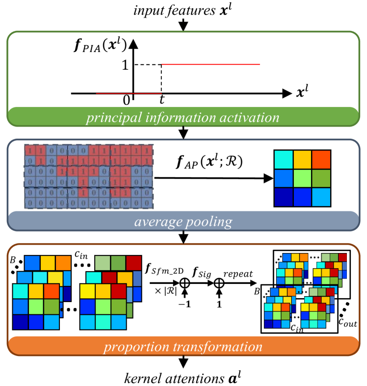
Figure 3: The pipeline of contextual attention generation module $\boldsymbol{f}_{CAG}$ in IKM, which is designed to generate kernel attention weights by inferring the global contextual information of feature map.

Different from the channel attention and spatial attention, IKM needs a 2D matrix of the same size as the kernel. Thus we generate the attention weights $\{\boldsymbol{a}_{j,i}\}$ by using a Contextual Attention Generation module (CAG) $\boldsymbol{f}_{CAG}(\cdot)$, as

$$\boldsymbol{a}^{l}=\boldsymbol{f}^{l}_{CAG}(\boldsymbol{x}^{l})=\boldsymbol{f}^{l}_{PT}(\boldsymbol{f}^{l}_{AP}(\boldsymbol{f}^{l}_{PIA}(\boldsymbol{x}^{l});\mathcal{R}))$$ (9)

where, as illustrated in Fig. 3, CAG consists of three parts for different purposes, i.e.,

i) Principal information activation $\boldsymbol{f}^{l}_{PIA}$. $\boldsymbol{f}^{l}_{PIA}$ is utilized to sample the dominating pixels to represent the principal contextual information. Specifically, we exploit a hard threshold strategy for principal information marking, which is formulated as

$$\boldsymbol{f}^{l}_{PIA}(\boldsymbol{x}_{i}^{l})=\left\{\begin{matrix}1&,\boldsymbol{x}_{i}^{l}\geq t\\ 0&,\boldsymbol{x}_{i}^{l}<t\end{matrix}\right.$$ (10)

where $t$ is a predefined threshold to sample the dominating pixels, and we assign 1 on them as the principal information.

ii) Average pooling $\boldsymbol{f}^{l}_{AP}$. Since the principal information is activated by $\boldsymbol{f}^{l}_{PIA}$, we then apply the average pooling operation $\boldsymbol{f}^{l}_{AP}(\boldsymbol{f}^{l}_{PIA}(\boldsymbol{x}^{l});\mathcal{R})$ on the principal information map with output size of $\mathcal{R}$. In a sense, $\boldsymbol{f}^{l}_{AP}$ here is exploited to calculate the proportion of the dominating pixels in each local patch as in Fig. 3.

iii) Proportion transformation $\boldsymbol{f}^{l}_{PT}$. As Eq. (8), we need a group of attention weights $\boldsymbol{a}\in\mathbb{R}^{c_{out}\times c_{in}\times\mathcal{R}}$, then there are two conditions that need meet: (a) the attention weights should be at the size of ${c_{out}\times c_{in}\times\mathcal{R}}$; (b) the attention weights should be adapted into reasonable values to avoid gradient exploding. For these conditions, we then introduce the proportion transformation module $\boldsymbol{f}^{l}_{PT}$, which can be formulated as

$$\boldsymbol{a}^{l}=\boldsymbol{f}^{l}_{PT}(\boldsymbol{\hat{x}}^{l})=1+\boldsymbol{f}^{l}_{Sig}({|\mathcal{R}|}\boldsymbol{f}^{l}_{Sfm\_2D}(\boldsymbol{\hat{x}}^{l})-1)$$ (11)

where $\boldsymbol{\hat{x}}=\boldsymbol{f}^{l}_{AP}(\boldsymbol{f}^{l}_{PIA}(\boldsymbol{x}^{l});\mathcal{R})$. To meet the condition (b), we utilize the 2D Softmax function $\boldsymbol{f}^{l}_{Sfm\_2D}$ and Sigmoid transformation function $\boldsymbol{f}^{l}_{Sig}$ to generate reasonable values of attention. Furthermore, to meet condition (a), we repeat $\boldsymbol{f}^{l}_{PT}(\mathbf{\hat{x}}^{l})$ for $c^{l}_{out}$ times to match the size of $\{\boldsymbol{w}^{l}_{j,i}\}$, namely, $\boldsymbol{a}_{1,i}^{l}=\boldsymbol{a}_{2,i}^{l}=...=\boldsymbol{a}_{{{c}_{out}},i}^{l}$. Note that, as Eq. (11), $\boldsymbol{f}^{l}_{AP}$ is acting in a residual learning fashion, which is more feasible for optimization empirically.

Compared with the existing channel and spatial attention mechanisms, our IKM utilizes the global contextual information to generate a group of attention weights $\boldsymbol{a}$, and adaptively modulates the kernels for feature self-enhancement in local receptive field and input channels. In a sense, IKM is equipped with the superiorities of both spatial and channel attention.

Algorithm 1 IsO Algorithm in Mini-Batch Training
// Image-specific Optimization (IsO) on $l$-th layer
Input: $B$ features/images in a mini-batch $\{\boldsymbol{x}^{l}_{1},\boldsymbol{x}^{l}_{2},...,\boldsymbol{x}^{l}_{B}\}$, general convolutional weights $\boldsymbol{w}^{l}$, contextual attention generation module $\boldsymbol{f}^{l}_{CAG}$;
Output: optimized general convolutional weights $\boldsymbol{w}^{l}$, output features/images $\{\boldsymbol{y}^{l}_{1},\boldsymbol{y}^{l}_{2},...,\boldsymbol{y}^{l}_{B}\}$.
// Forward propagation
1. Generating image-specific attentions $\boldsymbol{a}^{l}$ as Eq.(9); 2. Repeat $\boldsymbol{a}^{l}$ as $[\boldsymbol{a}^{l},\boldsymbol{a}^{l},...,\boldsymbol{a}^{l}]_{c^{l}_{out}}$ of size $(B\times c^{l}_{out})\times c^{l}_{in}\times\mathcal{R}^{l}$; 3. Repeat $\boldsymbol{w}^{l}$ as $[\boldsymbol{w}^{l},\boldsymbol{w}^{l},...,\boldsymbol{w}^{l}]_{B}$ of size $(B\times c^{l}_{out})\times c^{l}_{in}\times\mathcal{R}^{l}$; 4. Modulate kernel weights as $$\boldsymbol{\hat{w}}^{l}=\boldsymbol{a}^{l}\cdot\boldsymbol{w}^{l}$$ (12) and $\boldsymbol{\hat{w}}^{l}$ is of size $(B\times c^{l}_{out})\times c^{l}_{in}\times\mathcal{R}^{l}$; 5. Output features/images using group convolutions as $$\boldsymbol{y}^{l}=GroupConv(\boldsymbol{x}^{l};\boldsymbol{\hat{w}}^{l},groups=B)$$ (13)
// Backward propagation
1. Under the guidance of objective function $\boldsymbol{\mathcal{L}}$, the gradient in $l$-th layer should be $$g^{l}=\frac{\partial\boldsymbol{\mathcal{L}}}{\partial\boldsymbol{x}^{l}}\frac{\partial\boldsymbol{x}^{l}}{\partial{\boldsymbol{\hat{w}}}^{l}}$$ (14) but it is infeasible to use $\frac{\partial\boldsymbol{x}^{l}}{\partial{\boldsymbol{\hat{w}}}^{l}}\in\mathbb{R}^{(B\times c^{l}_{out})\times c^{l}_{in}\times\mathcal{R}^{l}}$ to optimize the parameter ${\boldsymbol{w}}^{l}\in\mathbb{R}^{c^{l}_{out}\times c^{l}_{in}\times\mathcal{R}^{l}}$. Then 2. Unfold $\frac{\partial\boldsymbol{x}^{l}}{\partial{\boldsymbol{\hat{w}}}^{l}}$ as $\frac{\partial\boldsymbol{x}^{l}}{\partial{\boldsymbol{\hat{w}}}^{l}}\in\mathbb{R}^{B\times c^{l}_{out}\times c^{l}_{in}\times\mathcal{R}^{l}}$; 3. Calculate the gradients as $$g^{l}=\frac{\partial\boldsymbol{\mathcal{L}}}{\partial\boldsymbol{x}^{l}}\sum_{b=1}^{B}(\frac{\partial\boldsymbol{x}^{l}}{\partial{\boldsymbol{\hat{w}}}^{l}})_{b}$$ (15) 4. Optimize the parameters $\boldsymbol{w}^{l}$ using $g^{l}$.

III-B Image-specific optimization

As aforementioned, each image should generate its specific contextual attention to adaptively modulate the kernels. However, in mini-batch training, the kernel weights $\{\boldsymbol{w}^{l}\}$ is of size $c^{l}_{out}\times c^{l}_{in}\times\mathcal{R}^{l}$ and independent of batch-wise dimension, but the attention $\{\boldsymbol{a}^{l}\}$ from Eq. (11) is of size $B\times c^{l}_{out}\times c^{l}_{in}\times\mathcal{R}^{l}$ where $B$ denotes the batch size.Thus, it is infeasible to backward the gradient in general mini-batch optimization, e.g., stochastic gradient descent (SGD). Therefore, in Algorithm 1, we propose an image-specific optimization (IsO) algorithm for mini-batch training, which is feasible to implement the optimization of modulated kernels and effectively backward propagate the image-specific attention weights, both of which positively guide the optimization of our IKM model.

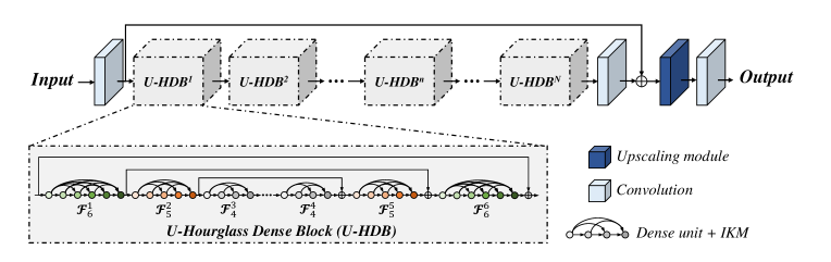
Figure 4: The framework of the proposed U-HDN backbone, which stacks a chain of U-hourglass dense blocks (U-HDB).

III-C U-Hourglass Dense Network

Since the attentions are repeated $c_{out}$ times to expand into the size of the kernel, the output channel should be lower to avoid reducing the diversity of attentions. Therefore, in this section, we mainly introduce an effective U-hourglass dense network (U-HDN) to utmost improve the effectiveness of IKM.

As a solution, dense connection has been demonstrated to be an excellent strategy to improve the information flow between layers with concatenated features, as in DenseNet [16]:

$${{\boldsymbol{x}}^{l+1}}=\boldsymbol{f}^{l}_{Composite}([{{\boldsymbol{x}}^{0}},{{\boldsymbol{x}}^{1}},...,{{\boldsymbol{x}}^{l}}])$$ (16)

where $\boldsymbol{f}^{l}_{Composite}(\cdot)$ indicates the $l$-th composite function which consists of a $3\times 3$ convolution and ReLU. Since the number of parameters increases by a large margin with the accumulated inputs, the growth rate $g$ is then applied to reduce the dimension of feature maps. Besides, a transition layer $\boldsymbol{f}_{Transition}(\cdot)$ is applied in the tail of dense unit for reducing the accumulated information flows to a single tensor $y$ with $c$ channels by a $1\times 1$ convolution layer without ReLU:

$${\boldsymbol{y}}=\boldsymbol{f}_{Transition}([{{\boldsymbol{x}}^{0}},{{\boldsymbol{x}}^{1}},...,{{\boldsymbol{x}}^{l}},{{\boldsymbol{x}}^{l+1}}])$$ (17)

As considered that the dimension in output channel $c_{out}$ should be lower to avoid reducing the diversity of attention, it is better to rich the input features and reduce the output features for more informative attention. Therefore, the dense unit is expected to be an appropriate architecture to improve the effectiveness of IKM.

Furthermore, to improve the effectiveness of dense connection, we then design a U-hourglass dense network (U-HDN) by stacking $N$ U-hourglass dense blocks as illustrated in Fig. 4. Particularly, different from the conventional dense blocks in DenseNet [16], we design the U-hourglass dense block (U-HDB) with two major amelioration:

III-C1 U-style residual learning

Residual learning [15] has been widely applied to facilitate training very deep networks, and has been demonstrated to be effective with dense connection by building the residual dense block (RDB) [26]. However, from Eq.(17), information flow in each layer is fed into the transition layer as identity, then

$${\boldsymbol{y}_{j}} =\sum\limits_{i=1}^{c+(l+1)\cdot g}{{{\boldsymbol{x}}_{i}}\cdot{{\boldsymbol{w}}_{j,i}}}=\sum\limits_{i=1}^{c}{{{\boldsymbol{x}}_{i}}\cdot{{\boldsymbol{w}}_{j,i}}}+\sum\limits_{i=c+1}^{c+(l+1)\cdot g}{{{\boldsymbol{x}}_{i}}\cdot{{\boldsymbol{w}}_{j,i}}}$$ (18)

$$={\boldsymbol{x}^{0}}\otimes{\boldsymbol{w}_{j,1:c}}+[{\boldsymbol{x}^{1}},{\boldsymbol{x}^{2}},...,{\boldsymbol{x}^{l+1}}]\otimes{\boldsymbol{w}_{j,c+1:c+(l+1)\cdot g}}$$

where $\{\boldsymbol{x}_{i}\}$ indicates the accumulated information flows and is formulated as $\{\boldsymbol{x}_{i}\}=[\boldsymbol{x}^{0}_{i},\boldsymbol{x}^{1}_{i},...,\boldsymbol{x}^{l+1}_{i}]$, $\{\boldsymbol{w}_{j,i}\}$ denotes $1\times 1$ kernel weight of transition layer $\boldsymbol{f}_{Transition}$.

Then, the vanilla input feature $\boldsymbol{x}^{0}$ is straightly propagated as a part of output without any non-linear transformation, in a sense, every single dense unit could be seen as a single layer on part of channels. Then if we directly introduce the residual learning for a single dense unit as residual dense block (RDB) (as illustrated in Fig. 7), the ability of non-linear representation in the dense unit would be largely discounted.

Therefore, we suggest each residual branch has to stack more than two dense units for powerful non-linear representation, and design a more effective U-style residual learning by stacking two symmetric dense units as in Fig. 4 and Fig. 7.

III-C2 Hourglass dense block learning

As illustrated in Fig. 4, we utilize an hourglass structure in the residual branch. We denote each dense unit by $\boldsymbol{\mathcal{F}}^{m}_{d_{m}}(\cdot)$, where $m$ and $d_{m}$ represent the $m$-th dense unit and the corresponding depth respectively, then the feed-forward procedure could be formulated as

$$\boldsymbol{y}=\boldsymbol{x}+\boldsymbol{\mathcal{F}}_{{{d}_{M}}}^{M}(\boldsymbol{\mathcal{F}}_{{{d}_{1}}}^{1}(\boldsymbol{x})+\boldsymbol{\mathcal{F}}_{{{d}_{M-1}}}^{M-1}(\boldsymbol{\mathcal{F}}_{{{d}_{2}}}^{2}(\boldsymbol{\mathcal{F}}_{{{d}_{1}}}^{1}(\boldsymbol{x}))+...))$$ (19)

in this case, the information flow of head unit $\boldsymbol{\mathcal{F}}_{{{d}_{1}}}^{1}(\boldsymbol{x})$ is transmitted straightly into tail unit $\boldsymbol{\mathcal{F}}_{{{d}_{M}}}^{M}$ through the residual branch, and also partly into the other intermediate units through dense connection as illustrated in Eq. (18). Besides, intuitively, the whole information flow of the tail unit works as the residues in such residual learning. In a sense, for a U-HDB with $M$ dense units, the desired residual features largely depend on the head unit $\boldsymbol{\mathcal{F}}_{{{d}_{1}}}^{1}$ and the tail unit $\boldsymbol{\mathcal{F}}_{{{d}_{M}}}^{M}$. Moreover, in Eq.(17), the deeper dense unit, the more accumulated features to make more informative outputs.

Therefore, deeper head and tail units are of great advantages to generate informative residues. Then, it is feasible to compress the computational complexities in the intermediate parts of U-HDB to get improvement with relatively fewer parameters. Therefore, as in Fig. 4, we set $d_{M-i+1}=d_{i}$ and $d_{j}>d_{i}$ for $i=1,2,...,M/2,j<i$ in hourglass dense block learning, which is symmetric as an hourglass.

TABLE I:
Quantitative comparisons with the state-of-the-art lightweight (#Params$\leq$2.0M or #FLOPs$\leq$100G) SISR methods.

Scale	Method	#Params	#FLOPs	Set5	Set14	BSD100	Urban100	Manga109
		(K)	(G)	PSNR/SSIM	PSNR/SSIM	PSNR/SSIM	PSNR/SSIM	PSNR/SSIM
$\times 2$	Bicubic	-	-	33.64 / 0.9292	30.22 / 0.8683	29.55 / 0.8425	26.87 / 0.8397	30.80 / 0.9339
	SRCNN [19]	8.0	1.4	36.66 / 0.9542	32.47 / 0.9069	31.37 / 0.8879	29.52 / 0.8947	35.73 / 0.9675
	VDSR [20]	664.7	115.1	37.53 / 0.9587	33.05 / 0.9127	31.90 / 0.8960	30.77 / 0.9141	37.37 / 0.9737
	LapSRN [49]	435.3	18.9	37.52 / 0.9591	32.99 / 0.9124	31.80 / 0.8949	30.41 / 0.9101	37.27 / 0.9740
	DRRN [22]	297.2	1275.5	37.74 / 0.9591	33.25 / 0.9137	32.05 / 0.8973	31.23 / 0.9188	37.88 / 0.9750
	IDN [45]	715.3	31.0	37.83 / 0.9600	33.30 / 0.9148	32.08 / 0.8985	31.27 / 0.9196	38.02 / 0.9749
	CARN [47]	1592.1	41.9	37.90 / 0.9602	33.58 / 0.9175	32.12 / 0.8987	31.95 / 0.9265	38.11 / 0.9764
	IMDN [51]	694.4	29.9	38.00 / 0.9605	33.63 / 0.9177	32.19 / 0.8996	32.13 / 0.9282	38.87 / 0.9774
	CFSRCNN [52]	1310.4	87.1	37.93 / 0.9603	33.63 / 0.9176	32.15 / 0.8997	32.13 / 0.9283	38.33 / 0.9765
	DeFiANS [36]	1027.6	44.2	38.03 / 0.9605	33.63 / 0.9181	32.20 / 0.8997	32.20 / 0.9286	38.91 / 0.9775
	U-HDN+IKM(Ours)	1390.9	60.3	38.06 / 0.9607	33.77 / 0.9191	32.24 / 0.9004	32.32 / 0.9301	39.09 / 0.9780
$\times 3$	Bicubic	-	-	30.40 / 0.8686	27.54 / 0.7741	27.21 / 0.7389	24.46 / 0.7349	26.95 / 0.8565
	SRCNN [19]	8.0	1.4	32.75 / 0.9090	29.29 / 0.8215	28.41 / 0.7863	26.24 / 0.7991	30.56 / 0.9125
	VDSR [20]	664.7	115.1	33.66 / 0.9213	29.78 / 0.8318	28.83 / 0.7976	27.14 / 0.8279	32.13 / 0.9348
	LapSRN [49]	435.3	8.5	33.82 / 0.9227	29.79 / 0.8320	28.82 / 0.7973	27.07 / 0.8271	32.21 / 0.9344
	DRRN [22]	297.2	1275.5	34.02 / 0.9244	29.98 / 0.8350	28.95 / 0.8004	27.54 / 0.8378	32.72 / 0.9380
	IDN [45]	715.3	13.8	34.12 / 0.9253	29.99 / 0.8356	28.95 / 0.8013	27.42 / 0.8360	32.71 / 0.9379
	CARN [47]	1592.1	22.3	34.33 / 0.9267	30.30 / 0.8416	29.07 / 0.8044	28.05 / 0.8499	33.32 / 0.9436
	IMDN [51]	703.1	13.5	34.36 / 0.9270	30.32 / 0.8417	29.09 / 0.8046	28.17 / 0.8519	33.61 / 0.9445
	CFSRCNN [52]	1495.0	63.7	34.32 / 0.9269	30.35 / 0.8423	29.07 / 0.8046	28.08 / 0.8507	33.44 / 0.9436
	DeFiANS [36]	1073.7	20.6	34.42 / 0.9273	30.34 / 0.8410	29.12 / 0.8053	28.20 / 0.8528	33.72 / 0.9447
	U-HDN+IKM(Ours)	1402.4	27.2	34.43 / 0.9273	30.39 / 0.8424	29.14 / 0.8060	28.19 / 0.8537	33.85 / 0.9459
$\times 4$	Bicubic	-	-	28.42 / 0.8101	25.99 / 0.7023	25.96 / 0.6672	23.14 / 0.6573	24.89 / 0.7866
	SRCNN [19]	8.0	1.4	30.49 / 0.8629	27.51 / 0.7519	26.91 / 0.7104	24.53 / 0.7230	27.66 / 0.8566
	VDSR [20]	664.7	115.1	31.35 / 0.8838	28.02 / 0.7678	27.29 / 0.7252	25.18 / 0.7525	28.87 / 0.8865
	LapSRN [49]	435.3	4.8	31.52 / 0.8854	28.09 / 0.7687	27.31 / 0.7255	25.21 / 0.7545	29.08 / 0.8883
	DRRN [22]	297.2	1275.5	31.67 / 0.8888	28.22 / 0.7721	27.38 / 0.7284	25.45 / 0.7639	29.44 / 0.8943
	IDN [45]	715.3	7.7	31.81 / 0.8903	28.25 / 0.7731	27.41 / 0.7295	25.41 / 0.7630	29.42 / 0.8939
	CARN [47]	1592.1	17.1	32.15 / 0.8948	28.58 / 0.7813	27.58 / 0.7360	26.03 / 0.7840	30.34 / 0.9079
	IMDN [51]	715.2	7.7	32.21 / 0.8946	28.58 / 0.7804	27.56 / 0.7352	26.04 / 0.7838	30.45 / 0.9072
	MS3-Conv [48]	1300.0	21.6	32.09 / 0.8945	28.61 / 0.7821	27.59 / 0.7368	26.09 / 0.7859	- / -
	CFSRCNN [52]	1458.1	58.7	32.10 / 0.8932	28.63 / 0.7814	27.55 / 0.7346	26.06 / 0.7836	30.43 / 0.9068
	DeFiANS [36]	1064.5	12.8	32.16 / 0.8942	28.63 / 0.7810	27.58 / 0.7363	26.10 / 0.7862	30.59 / 0.9084
	U-HDN+IKM(Ours)	1400.1	15.7	32.29 / 0.8955	28.68 / 0.7826	27.62 / 0.7373	26.17 / 0.7880	30.85 / 0.9110

IV Experiments

IV-A Datasets and Evaluation

Following the existing single image SR researches, we implement our experiments on several benchmark datasets for evaluation: Set5 [53], Set14 [6], BSD100 [54] and Manga109 [49] datasets. And in the training phase, 3450 high-quality images from DIV2K and Flickr2K [55] dataset are considered and down-sampled using Bicubic algorithm to generate the HR-LR pairs. In detail, we use the $48\times 48$ RGB patches from the low-resolution training set as input and the corresponding $48s\times 48s$ high-resolution patches as ground-truth for $\times s$ upscaling, and augment these LR-HR pairs with randomly horizontal flips and 90 rotations. Particularly, all the LR and HR images are pre-processed by subtracting the mean RGB value of the training sets.

To evaluate the SR performance, we apply two full-reference image quality assessment (IQA) criteria: Peak Signal-to-Noise Ratio (PSNR) and Structural SIMilarity (SSIM). And following the convention of SR, only the luminance channel is selected for full-reference image quality assessment because the intensity of image is more sensitive to human vision than the chroma channels. Moreover, we use two criteria to represent the computational complexities: #Params (space complexity) denotes the number of parameters, and #FLOPs (time complexity) indicates the number of operations by Multi-Adds which is the number of composite multiply-accumulate operations for generating a $480\times 360\times 3$ output.

IV-B Implementation Details

IV-B1 Hyperparameters

As illustrated in Section III-C, we stack $N$=$4$ U-HDBs to build a lightweight U-HDN with only 1.4M parameters. And in each U-HDB, by applying U-style residual learning and hourglass dense block learning, $M$=$6$ dense units are stacked with symmetric depth of $[6,5,4,4,5,6]$, where the growth rate $g$=$12$ and input channel in head layer $C$=$64$. Furthermore, IKM is applied into each layer of U-HDN except for the transition layers, and the threshold of $\boldsymbol{f}_{PIA}$ is set to $t$=$0$. Besides, we utilize the sub-pixel convolutions [30] for feature upscaling in the upscaling module as in Fig. 4.

IV-B2 Optimization

All of our models are optimized via minimizing the mean absolute error (MAE) between the super-resolved image $\boldsymbol{f}_{model}(\boldsymbol{x})$ and the corresponding ground-truth HR $\boldsymbol{y}$. Therefore, given a training dataset $\{\boldsymbol{x}^{b},\boldsymbol{y}^{b}\}^{B}_{b=1}$, where $B$ is the batch size and $\{\boldsymbol{x}^{b},\boldsymbol{y}^{b}\}$ are the $b$-th LR and HR patch pairs. Then, the objective function is formulated as

$$\boldsymbol{\mathcal{L}}(\Theta)=\sum_{b=1}^{B}\left\|\boldsymbol{y}^{b}-\boldsymbol{f}_{model}(\boldsymbol{x}^{b};\Theta)\right\|_{1}$$ (20)

where $\Theta$ denotes the trainable parameters of models, which are optimized by using the Adam optimizer [56] with mini-batches of size $B=16$, with the learning rate being initialized to ${{10}^{-4}}$ and halved for every $10^{5}$ mini-batch updates. Each of the final models will get convergence after $3\times 10^{5}$ updates on the PyTorch framework and a 32GB NVIDIA Tesla V100 GPU.

IV-C Comparison with State-of-the-art Methods

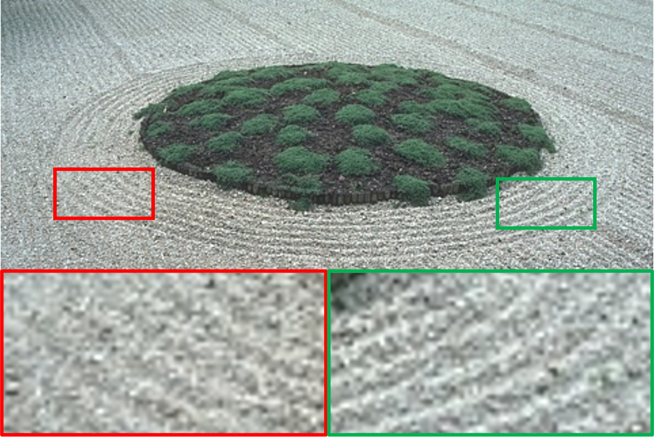
(a) HR Ground-truth
PSNR / SSIM

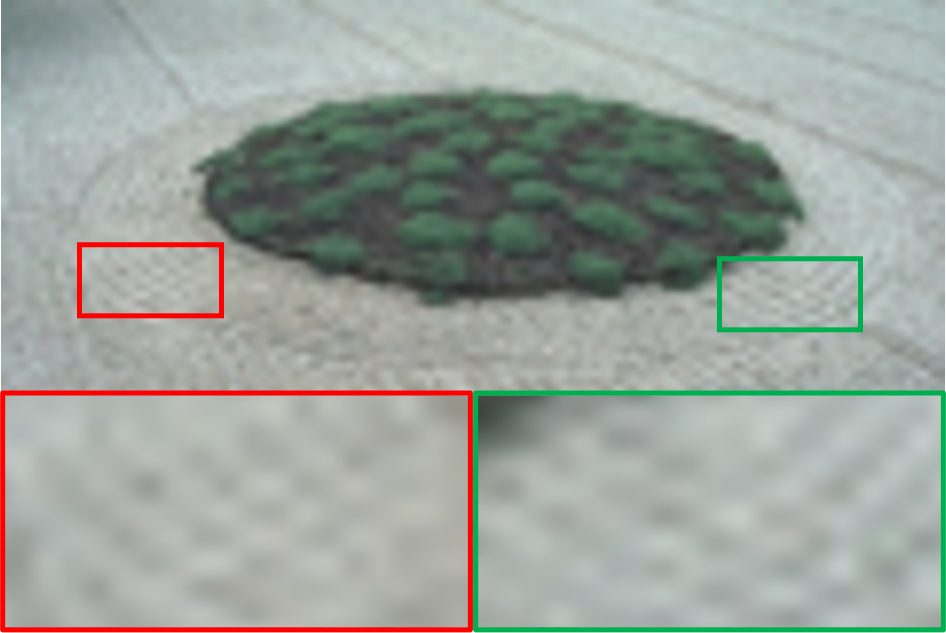
(b) Bicubic
21.78 / 0.2696

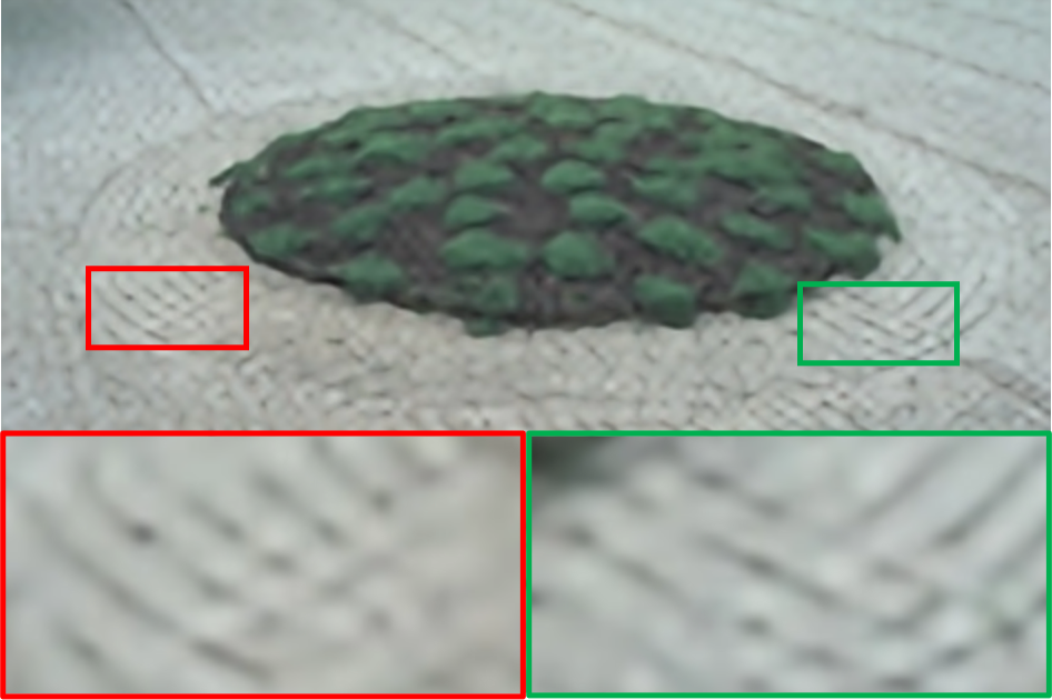
(c) SRCNN [19]
21.87 / 0.3051

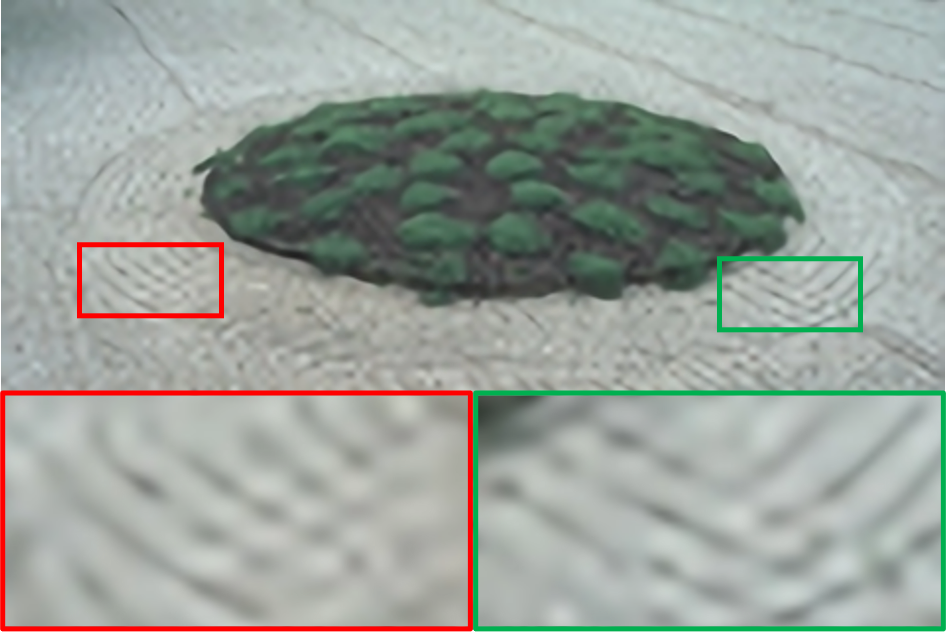
(d) VDSR [20]
21.90 / 0.3115

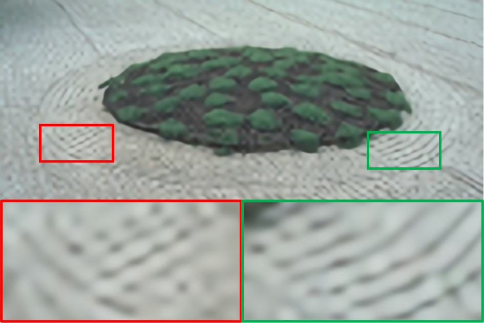
(e) CARN [47]
21.90 / 0.3136

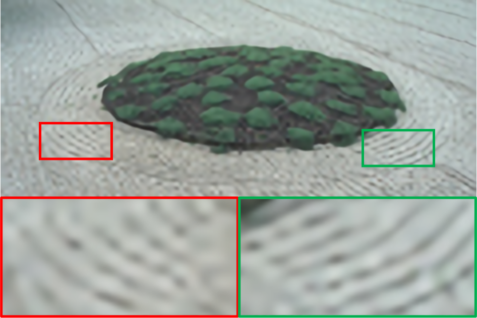
(f) U-HDN+IKM (Ours)
21.94 / 0.3176

Figure 5: Subjective quality assessment for $\times 4$ upscaling on image: “86016” from BSD100 dataset. Obviously, the global composition of this image is lying on the center region with lower illuminance, so the IKM attention weight seems as an “isotropic Laplace operator” and keeps the edges well-preserved.

(a) HR Ground-truth
PSNR / SSIM

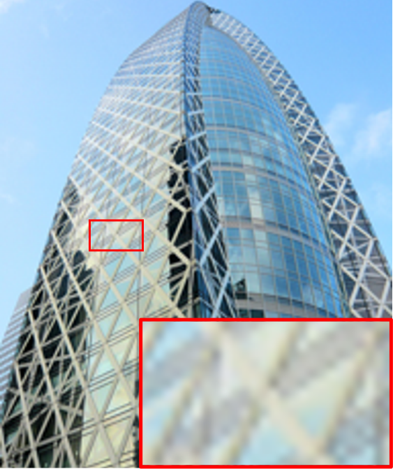
(b) Bicubic
20.86 / 0.5794

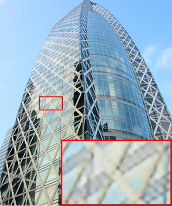
(c) SRCNN [19]
21.69 / 0.6464

(d) VDSR [20]
22.26 / 0.6874

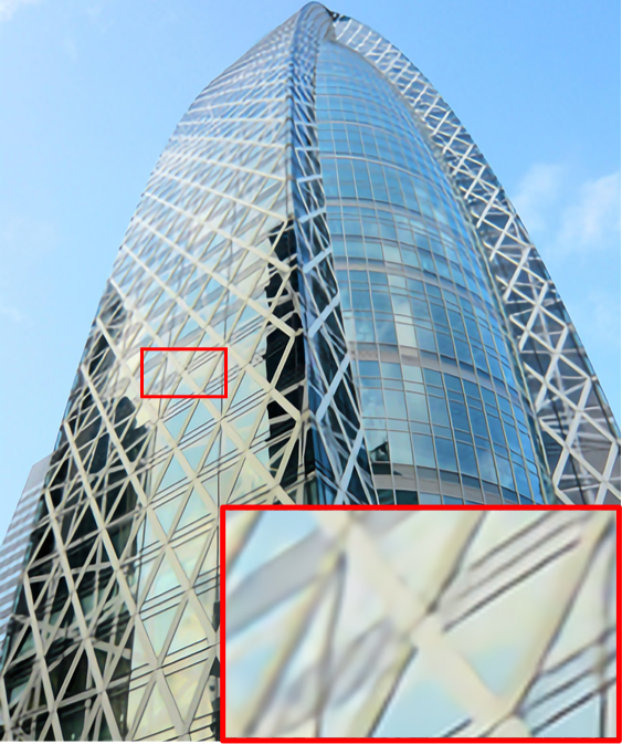
(e) CARN [47]
23.18 / 0.7482

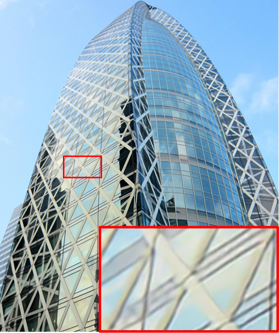
(f) U-HDN+IKM(Ours)
23.23 / 0.7535

Figure 6: Subjective quality assessment for $\times 4$ upscaling on image: “img039” from Urban100 dataset. Obviously, the global composition of this image shows higher contrasts in the vertical direction, so the IKM attention weight seems as an “horizontal Prewitt operator”, which suppresses the distortions and keeps the vertical edges well-preserved.

TABLE II:
Quantitative comparisons with the state-of-the-art high-fidelity SISR methods for $\times 2$ upscaling.

Method	#Params	#FLOPs	Set5	Set14	BSD100	Urban100	Manga109
	(M)	(G)	PSNR/SSIM	PSNR/SSIM	PSNR/SSIM	PSNR/SSIM	PSNR/SSIM
Bicubic	-	-	33.64 / 0.9292	30.22 / 0.8683	29.55 / 0.8425	26.87 / 0.8397	30.80 / 0.9339
U-HDN+IKM(Ours)	1.39	60.3	38.06 / 0.9607	33.77 / 0.9191	32.24 / 0.9004	32.32 / 0.9301	39.09 / 0.9780
EDSR [23]	40.7	1760.0	38.11 / 0.9600	33.82 / 0.9189	32.33 / 0.9011	32.94 / 0.9351	39.10 / 0.9773
RDN [26]	5.62	243.0	38.16 / 0.9603	33.88 / 0.9199	32.31 / 0.9009	32.89 / 0.9353	39.09 / 0.9771
RCAN [31]	15.4	663.5	38.18 / 0.9604	34.00 / 0.9203	32.37 / 0.9016	33.14 / 0.9364	39.34 / 0.9777
OISR-RK3 [57]	44.3	1812.1	38.13 / 0.9602	33.81 / 0.9194	32.34 / 0.9011	33.00 / 0.9357	39.13 / 0.9773
CSFM [33]	12.1	519.9	38.17 / 0.9605	33.94 / 0.9200	32.34 / 0.9013	33.08 / 0.9358	39.30 / 0.9775
U-HDNL+IKM(Ours)	10.9	471.5	38.23 / 0.9614	34.03 / 0.9217	32.35 / 0.9018	32.84 / 0.9346	39.46 / 0.9788

IV-C1 Comparison of full models

As described in Section IV-B1, the default settings are defined for lightweight applications, then several state-of-the-art lightweight (#Params$\leq$2.0M or #FLOPs$\leq$100G) SR methods (e.g., SRCNN [19], VDSR [20], LapSRN [49], DRRN [22], IDN [45], CARN [47], IMDN [51], MS³-Conv [48], CFSRCNN [52] and DeFiAN_S [36]) are selected to compare with our “UHDN+IKM”. Besides, based on the default settings in Section IV-B1, we also build a larger model “UHDN_L+IKM” by resetting $N$=$8$, $g$=$24$ and $C$=$128$ for high-fidelity application, and compare it with the state-of-the-art high-fidelity SR methods (e.g., EDSR [23], RDN [26], RCAN [31], OISR-RK3 [57] and CSFM [33]).

To evaluate the pixel-wise information fidelity and the computational complexities, we conduct the experimental comparisons on the proposed method and other state-of-the-art SISR methods, and the quantitative full-reference IQA results are reported in TABLE I and TABLE II. Particularly, since no additional parameters need to be optimized in IKM, both of the lightweight “U-HDN+IKM” and high-fidelity “U-HDN_L+IKM” achieve relative best performances with lower computational complexities against other state-of-the-art SISR methods. Moreover, we also post up the super-resolved results in chromatic format for subjective quality assessment as Fig. 5 and Fig. 6 show. By introducing the image-specific attentions to modulate the convolutional kernels, our methods are adaptive to reconstruct different images with the corresponding specific kernels. Particularly, in Fig. 5, the global contextual composition of the image is lying on the center with lower illuminance, so the IKM attention weight acts as an “isotropic Laplace operator” and keeps the edges well-preserved. And in Fig. 6, the composition of the image shows higher contrasts in vertical directions, so the IKM attention weight acts as an “horizontal Prewitt operator”, which suppresses the distortions and keeps the vertical edges well-preserved.

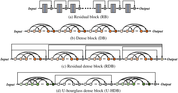
Figure 7: Comparison of U-hourglass dense block (U-HDB) and other state-of-the-art architectures, including: (a) residual block (RB) in EDSR [23]; (b) dense block (DB) in SRDenseNet [24] and MemNet [25]; (c) residual dense block (RDB) in RDN [26].

IV-C2 Comparison of architectures

Aiming at demonstrating the effectiveness of the proposed architectures (U-HDN and IKM), we apply several state-of-the-art architectures into the same backbone by stacking $N=1$ blocks, and then train these models with $5\times 10^{4}$ mini-batch updates. The architectures are shown in Fig. 7 and specified as following:

TABLE III:
Comparisons with state-of-the-art
architectures for $\times 2$ upscaling on Set5 dataset.

Architectures		#Params (K)		#FLOPs (G)		PSNR / SSIM
RB[23]	-	362.1	+0	15.8	+0	37.47 / 0.9584
	+CA[31]		+19.4		+$\approx$0	37.53 / 0.9586
	+SA[33]		+9.62		+0.42	37.52 / 0.9586
	+IKM (Ours)		+0		+$\approx$0	37.52 / 0.9586
DB[24]	-	382.3	+0	16.7	+0	37.44 / 0.9583
	+CA[31]		+2.61		+$\approx$0	37.46 / 0.9585
	+SA[33]		+1.29		+0.06	37.48 / 0.9585
	+IKM (Ours)		+0		+$\approx$0	37.52 / 0.9586
RDB[26]	-	411.0	+0	18.0	+0	37.48 / 0.9584
	+CA[31]		+2.61		+$\approx$0	37.48 / 0.9586
	+SA[33]		+1.29		+0.06	37.53 / 0.9586
	+IKM (Ours)		+0		+$\approx$0	37.55 / 0.9587
U-HDB (Ours)	-	384.9	+0	16.9	+0	37.48 / 0.9585
	+CA[31]		+2.61		+$\approx$0	37.47 / 0.9585
	+SA[33]		+1.29		+0.06	37.52 / 0.9586
	+IKM (Ours)		+0		+$\approx$0	37.57 / 0.9588

i) Residual block (RB). To train very deep networks, residual learning is introduced for image classification in ResNet [15] and extended for image super-resolution (SR) in EDSR [23] and DRRN [22]. In this section, we stack $M=8$ enhanced residual block (RB) with $C=48$ in each residual block to build a deep but relatively lightweight network to compare with our U-HDB.

ii) Dense block (DB). To improve the feature diversity, the dense connection is proposed for visual classification in DenseNet [16] and extended for SR in SRDenseNet [24]. Similar to SRDenseNet but with some modifications, we apply a group of dense units with the same depth $d$=5 in each block of backbone, and set the growth rate $g$=12 as our U-HDN.

iii) Residual dense block (RDB). To exploit both characteristics of residual learning and dense connection, Zhang et al. [26] propose the residual dense network with RDBs, which achieves the state-of-the-art performance. Different from SRDenseNet, RDN embeds the dense unit into the residual learning structure, and then utilizes the global feature fusion module (implemented as the transition layer $\boldsymbol{f}_{Transition}(\cdot)$ in DenseNet) in the tail of network for intermediate features fusion. For a fair comparison, we apply the backbone of RDN in each block and set the growth gate $g$=12.

iv) U-hourglass dense block (U-HDB). Aiming at further improving the feature diversity, we propose the U-HDB by stacking symmetrically hourglass dense units with U-style residual learning, which is expected to be an appropriate architecture for utmost improvement of utilizing IKM theoretically and achieves the state-of-the-art performance against the prior methods as illustrated in the paper.

As in TABLE III, even using the vanilla conventional convolution, the proposed U-HDB reaches relatively better performance than the other state-of-the-art architectures, and by further applying the IKM, all the architectures achieve relatively higher improvements than applying channel attention (CA) or spatial attention (SA).

IV-D Model Analysis

In this subsection, we mainly conduct some ablation studies and model analysis with experimental demonstrations. Specifically, the models in this section are trained with $5\times 10^{4}$ mini-batch updates on DIV2K datasets under the settings as $N=4$, $M=6$ with depth of $[6,5,4,4,5,6]$, $C=64$, $g=12$, unless otherwise specified.

IV-D1 Effect of model size

As illustrated in Section IV-B1, our U-HDN (w/ IKM) is designed under several hyperparameters, including the number of U-HDBs $N$, the number of dense units in each U-HDB $M$, and the input channel in the head of dense unit $C$. We then conduct the model analysis on different settings of hyperparameters as in Fig. 8. In detail, the symmetric depths of U-HDBs are set to $[6,5,4,4,5,6]$ when $M=6$ or $[6,4,4,6]$ when $M=4$.

As shown in Fig. 8, we find that, as the model size increases (i.e., larger $N$, $M$, $C$ and symmetric depth of each U-HDB), the performance gets a large margin of improvement but reaches the bottleneck when the model size reaches a peak level. Therefore, we choose an appropriate setting of hyperparameter as described in Section IV-B1, which achieves excellent performance with relatively lower computational complexities.

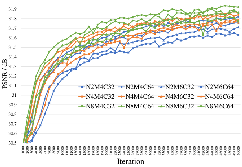
Figure 8: Effect of model size with different hyperparameters: average PSNR on BSD100 dataset for $\times 2$ upscaling. Note that, “N4M6C64” represents the U-HDN (w/ IKM) with $N=4$ U-HDBs, in each U-HDB, $M=6$ dense units are stacked with depthes of $[6,5,4,4,5,6]$ and the number of channels are $C=64$.

IV-D2 Effect of IKM

As illustrated in Section III-A, IKM is regarded as enhancing the input features with the modulated kernels as in Eqs. (8-9), we then conduct several investigations on the effects of the whole IKM module, the attention generation module $\boldsymbol{f}_{CAG}$, and the size of receptive field $\mathcal{R}$.

i) Investigations on performance. To demonstrate the effect of the proposed IKM, we apply the vanilla convolution, the variants with channel attention (CA), spatial attention (SA), or IKM into several architectures in Fig. 7. As reported in TABLE III, by applying our IKM, although without any additional parameters, the models possess a large margin of improvement for all the implemented architectures over the vanilla convolution, and achieve comparable performance with relatively lower complexity against the variants with channel attention and spatial attention. Particularly, as aforementioned in Section III-C, dense connection should be expected to be more appropriate for utmost improvement of utilizing IKM. We find the larger margin of improvements are arisen on the dense connections, i.e., 0.05dB for RB, but 0.08dB for DB, 0.07dB for RDB, and 0.09dB for U-HDB.

ii) Investigation on $\boldsymbol{f}_{CAG}$. To generate the image-specific layout of features, we introduce a layout generation module $\boldsymbol{f}_{CAG}$ into each IKM. So we also conduct investigations on the setting of $\boldsymbol{f}_{CAG}$, specifically, on the threshold in $\boldsymbol{f}_{PIA}$. As in Eq. (10) and Fig. 3, a hard threshold function is applied to sample the principal information of feature. Since the whole U-HDN model and U-HDBs work in a residual learning manner as in Fig. 4 and Fig. 7, most values in residual features are likely to be zero as described in [20]. So we suggest $t=0$ as the threshold to activate the principal information and next to sample them. And to demonstrate this assumption, we conduct some investigations on choosing an appropriate threshold as in Fig. 9. Specifically and intuitively, the median value of feature should be more appropriate than 0, however, median operation $torch.median()$ need to sort all atoms in each location of feature map, and is inefficient in parallel computing with GPUs especially for large patches.

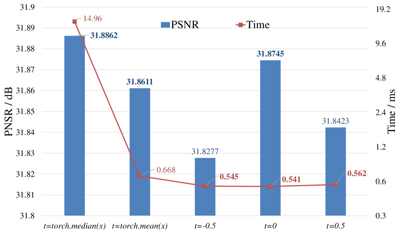
Figure 9: Investigation on threshold $t$ of $\boldsymbol{f}_{PIA}$: average PSNR and execution time of $\boldsymbol{f}_{PIA}$ on BSD100 dataset for $\times 2$ upscaling.

TABLE IV:
Investigation on local receptive field $\mathcal{R}$
for $\times 2$ upscaling on BSD100 dataset.

Kernel	Dilation	$\mathcal{R}$	IKM	#Params	PSNR	SSIM
(K)	(D)
$3\times 3$	$1\times 1$	$3\times 3$	$\times$	1390.9	31.80	0.8951
			✓	1390.9	31.87	0.8960
$3\times 3$	$2\times 2$	$5\times 5$	$\times$	1390.0	31.72	0.8945
			✓	1390.0	31.79	0.8954
$3\times 3$	$3\times 3$	$7\times 7$	$\times$	1390.0	31.61	0.8927
			✓	1390.9	31.71	0.8942
$5\times 5$	$1\times 1$	$5\times 5$	$\times$	3436.7	31.82	0.8952
			✓	3436.7	31.91	0.8968
$5\times 5$	$2\times 2$	$9\times 9$	$\times$	3436.7	31.69	0.8936
			✓	3436.7	31.83	0.8954
*$\mathcal{R}=K+(K-1)*(D-1)$.

iii) Investigation on local receptive field $\mathcal{R}$. As illustrated in Section III-A and Eq. (8), IKM is equivalent to introducing attentions to act on the local receptive fields of feature, we then investigate several settings of local receptive field while with or without IKM. In addition, in deep full convolutional networks, the receptive field depends on the settings of convolutional kernel (e.g., “kernel size”, “dilation”) and is calculated as $\mathcal{R}=K+(K-1)*(D-1)$ [58]. As reported in TABLE IV, with the local receptive field increases, IKM achieves higher gains on both PSNR and SSIM, e.g., when $\mathcal{R}=9\times 9$, the gain reaches 0.14dB on PSNR.

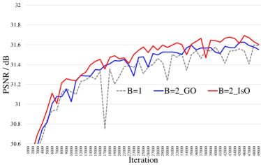
(a) B=2

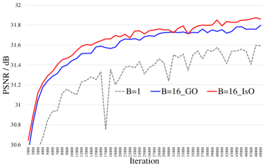
(b) B=16

Figure 10: Effect of IsO algorithm in mini-batch training: average PSNR on BSD100 dataset for $\times 2$ upscaling. As batch size increases, IsO shows higher superiority to general optimization (GO).

TABLE V:
Ablation study on U-HDN for $\times 2$ upscaling.

U-style residual learning		$\times$	✓	$\times$	✓
Hourglass dense block		$\times$	$\times$	✓	✓
Complexities	#Params(M)	1380.3	1380.3	1390.9	1390.9
	#FLOPs(G)	60.0	60.0	60.3	60.3
Set5	PSNR	37.50	37.61	37.54	37.65
	SSIM	0.9584	0.9588	0.9587	0.9590
BSD100	PSNR	31.80	31.84	31.82	31.87
	SSIM	0.8950	0.8956	0.8955	0.8960

IV-D3 Effect of IsO algorithm

As illustrated in Section III-A, each image should generate its specific contextual attention to adaptively recalibrate the kernel weights. We then introduce the image-specific optimization (IsO) in mini-batch training phase as described in Algorithm 1, which is a feasible algorithm to optimize kernel weights and effectively backward the image-specific layout attentions, both of which positively guide the optimization of model. To demonstrate the effectiveness of our IsO algorithm, we conduct several experiments on optimization with different mini-batches using IsO algorithm or general optimization (GO) algorithm.

As shown in Fig. 10, as the batch size increases, our IsO algorithm shows higher superiorities to general optimization. The main reason is that, in general optimization, when the batch size increases and the generated attentions are averaged into $\boldsymbol{a}\in\mathbb{R}^{c_{out}\times c_{in}\times\mathcal{R}}$, then the averaged attentions have lost the ability to represent the image-specific contextual information and only play a part on channel-wise recalibration as channel attention mechanism.

IV-D4 Investigation on U-HDN

As aforementioned in Section III-C, we design a new backbone U-HDN by stacking $N$=4 U-HDBs, which is a variant of dense block [16, 24] with two major amelioration: U-style residual learning and hourglass dense block. To investigate their effect, we conduct the ablation study on the U-HDB structure and report the comparative results in TABLE V and find that, both of the U-style residual learning and hourglass dense block play significant roles in improving the performances.

Furthermore, from Eq. (18), the output information flows (features) of each block have higher relevance to the head and tail dense units in the U-style residual learning, then it is better to rich these units with deeper structure, e.g., the depths in each block are set symmetrically as $[6,5,4,4,5,6]$. To demonstrate this assumption, we keep the U-style residual learning and design some variants of hourglass dense block with comparable parameters, including:

• “U-HDN” where the depthes in each block are symmetric as $[6,5,4,4,5,6]$ and the computational complexities are #Params=1390.9K and #FLOPs=60.3G;

• “U-HDN_V1” where the depthes in each block are symmetric as $[4,5,6,6,5,4]$ and the computational complexities are #Params=1390.9K and #FLOPs=60.3G;

• “U-HDN_V2” where the depthes in each block are ascending as $[2,3,4,5,6,7]$ and the computational complexities are #Params=1401.3K and #FLOPs=60.8G;

• “U-HDN_V3” where the depthes in each block are descending as $[7,6,5,4,3,2]$ and the computational complexities are #Params=1401.3K and #FLOPs=60.8G.

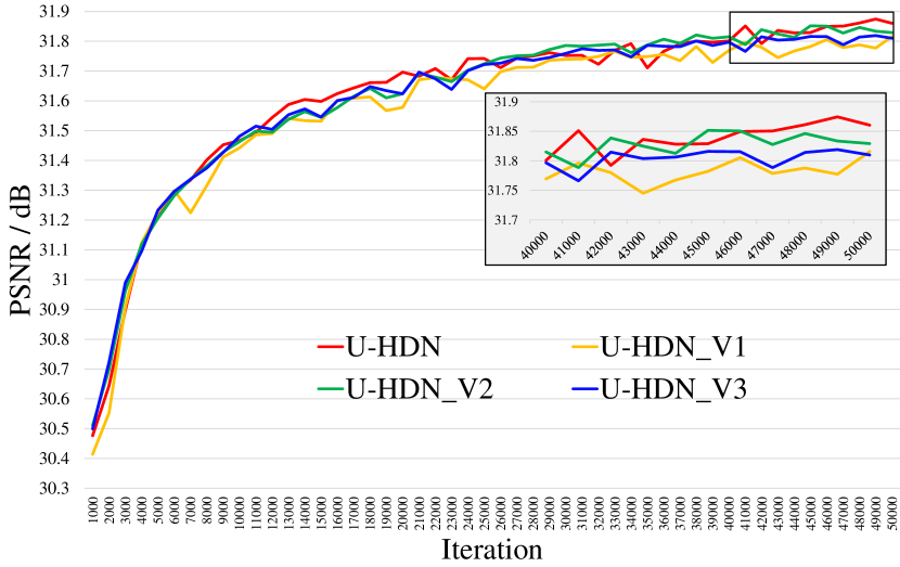
Figure 11: Effect of hourglass block learning in residual networks: average PSNR on BSD100 dataset for $\times 2$ upscaling. By increasing the capacity of head or/and tail units, model achieves better performance, i.e., “U-HDN”$>$“U-HDN_V2”$\approx$“U-HDN_V3”$>$“U-HDN_V1”.

As shown in Fig. 11, with comparable computational complexities, U-HDN shows superiority to other variants. Hence the assumption of hourglass dense block learning that “the desired residual features largely depend on the head and tail units” is experimentally demonstrated, and is promising to be exploited into other applications where use dense connection. For example, by increasing the capacity of the tail unit, “U-HDN_V2” and “U-HDN_V3” perform better than “U-HDN_V1” but worse than “U-HDN”.

IV-E Discussions

As mentioned above, since the IKM is an image-specific method to adaptively modulate the convolutional kernels in deep CNNs, we should use the IsO algorithm to optimize the model in mini-batch training, and utilize the group convolutions to infer the forward propagation as illustrated in Algorithm 1. However, the existing implementation of group convolutions is less efficient than general convolution. Therefore, in spite of no additional parameters, a model with IKM runs slower than the one without it. So it is expected to exploit an efficient variant of group convolutions to accelerate the forward propagation of IKM.

Additionally, as illustrated in Eq. (8), the image-specific attention weights $\boldsymbol{a}$ needs a 2D matrix at same size as kernel $\boldsymbol{w}$. There also exists a large range of choosing an appropriate strategy to generate such attention weight, so it is expected to exploit more types of image-specific attention weight.

V Conclusions

In this paper, to bridge the gap between the data-driven and image-specific SR methods, an image-specific convolutional kernel modulation (IKM) is proposed to adaptively modulate the convolutional kernels without any additional parameters, which achieves excellent performances against the vanilla convolution and several attention mechanisms, e.g., channel attention. Furthermore, on the optimization of IKM in mini-batch training, an image-specific optimization (IsO) algorithm is proposed and shows superiority to the general SGD optimization experimentally. Meanwhile, a U-hourglass dense network (U-HDN) is designed by utilizing U-style residual leaning and hourglass dense block learning, which are demonstrated to be appropriate architectures for utmost improving the effectiveness of IKM theoretically. Theoretical analysis and extensive experiments demonstrate the effectiveness and superiorities of the proposed methods.

References

- [1] R. Keys, “Cubic convolution interpolation for digital image processing,” IEEE Trans. Acoustics, Speech, and Signal Process., vol. 29, no. 6, pp. 1153–1160, 1981.
- [2] L. Zhang and X. Wu, “An edge-guided image interpolation algorithm via directional filtering and data fusion,” IEEE Trans. Image Process., vol. 15, no. 8, pp. 2226–2238, 2006.
- [3] A. Marquina and S. Osher, “Image super-resolution by tv-regularization and bregman iteration,” J. Sci. Comput., vol. 37, no. 3, pp. 367–382, Dec. 2008.
- [4] W. Dong, L. Zhang, G. Shi, and X. Wu, “Image deblurring and super-resolution by adaptive sparse domain selection and adaptive regularization,” IEEE Trans. Image Process., vol. 20, no. 7, pp. 1838–1857, Jul. 2011.
- [5] J. Yang, J. Wright, T. S. Huang, and Y. Ma, “Image super-resolution via sparse representation,” IEEE Trans. Image Process., vol. 19, no. 11, pp. 2861–2873, 2010.
- [6] R. Zeyde, M. Elad, and M. Protter, “On single image scale-up using sparse-representations,” in Curves and Surfaces, 2010.
- [7] R. Timofte, V. D. Smet, and L. V. Gool, “A+: Adjusted anchored neighborhood regression for fast super-resolution,” in Asian Conf. Comput. Vis., 2014, pp. 111–126.
- [8] Z. Zhu, F. Guo, H. Yu, and C. Chen, “Fast single image super-resolution via self-example learning and sparse representation,” IEEE Trans. Multimedia, vol. 16, no. 8, pp. 2178–2190, 2014.
- [9] Y. Hu, N. Wang, D. Tao, X. Gao, and X. Li, “Serf: A simple, effective, robust, and fast image super-resolver from cascaded linear regression,” IEEE Trans. Image Process., vol. 25, no. 9, pp. 4091–4102, 2016.
- [10] Y. Huang, J. Li, X. Gao, L. He, and W. Lu, “Single image super-resolution via multiple mixture prior models,” IEEE Trans. Image Process., vol. 27, no. 12, pp. 5904–5917, 2018.
- [11] Y. Lecun, L. Bottou, Y. Bengio, and P. Haffner, “Gradient-based learning applied to document recognition,” Proceedings of the IEEE, vol. 86, no. 11, pp. 2278–2324, Nov 1998.
- [12] A. Krizhevsky, I. Sutskever, and G. E. Hinton, “Imagenet classification with deep convolutional neural networks,” in Adv. Neural Inform. Process. Syst., 2012, pp. 1097–1105.
- [13] K. Simonyan and A. Zisserman, “Very deep convolutional networks for large-scale image recognition,” in Int. Conf. Learn. Represent., 2015.
- [14] C. Szegedy, W. Liu, Y. Jia, P. Sermanet, S. Reed, D. Anguelov, D. Erhan, V. Vanhoucke, and A. Rabinovich, “Going deeper with convolutions,” in IEEE Conf. Comput. Vis. Pattern Recog., 2015, pp. 1–9.
- [15] K. He, X. Zhang, S. Ren, and J. Sun, “Deep residual learning for image recognition,” in IEEE Conf. Comput. Vis. Pattern Recog., 2016, pp. 1063–6919.
- [16] G. Huang, Z. Liu, L. van der Maaten, and K. Q. Weinberger, “Densely connected convolutional networks,” in IEEE Conf. Comput. Vis. Pattern Recog., 2017, pp. 2261–2269.
- [17] J. Hu, L. Shen, and G. Sun, “Squeeze-and-excitation networks,” in IEEE Conf. Comput. Vis. Pattern Recog., 2018, pp. 7132–7141.
- [18] C. Dong, C. C. Loy, K. He, and X. Tang, “Learning a deep convolutional network for image super-resolution,” in Eur. Conf. Comput. Vis., 2014, pp. 184–199.
- [19] C. Dong, C. C. Loy, K. He and X. Tang, “Image super-resolution using deep convolutional networks,” IEEE Trans. Pattern Anal. Mach. Intell., vol. 38, no. 2, pp. 295–307, 2016.
- [20] J. Kim, J. K. Lee, and K. M. Lee, “Accurate image super-resolution using very deep convolutional networks,” in IEEE Conf. Comput. Vis. Pattern Recog., 2016, pp. 1646–1654.
- [21] C. Ledig, L. Theis, F. Huszár, J. Caballero, A. P. Aitken, A. Tejani, J. Totz, Z. Wang, and W. Shi, “Photo-realistic single image super-resolution using a generative adversarial network,” in IEEE Conf. Comput. Vis. Pattern Recog., Jul. 2017, pp. 105–114.
- [22] Y. Tai, J. Yang, and X. Liu, “Image super-resolution via deep recursive residual network,” in IEEE Conf. Comput. Vis. Pattern Recog., 2017, pp. 3147–3155.
- [23] B. Lim, S. Son, H. Kim, S. Nah, and K. M. Lee, “Enhanced deep residual networks for single image super-resolution,” in IEEE Conf. Comput. Vis. Pattern Recog. Worksh., 2017, pp. 136–144.
- [24] T. Tong, G. Li, X. Liu, and Q. Gao, “Image super-resolution using dense skip connections,” in Int. Conf. Comput. Vis., 2017, pp. 4799–4807.
- [25] Y. Tai, J. Yang, X. Liu, and C. Xu, “Memnet: A persistent memory network for image restoration,” in Int. Conf. Comput. Vis., 2017, pp. 4549–4557.
- [26] Y. Zhang, Y. Tian, Y. Kong, B. Zhong, and Y. Fu, “Residual dense network for image super-resolution,” in IEEE Conf. Comput. Vis. Pattern Recog., 2018, pp. 2472–2481.
- [27] Y. Zhang, Y. Tian, Y. Kong, B. Zhong, and Y. Fu, “Residual dense network for image restoration,” IEEE Trans. Pattern Anal. Mach. Intell., vol. 43, no. 7, pp. 2480–2495, 2021.
- [28] X. Zhang, P. Gao, S. Liu, K. Zhao, G. Li, L. Yin, and C. W. Chen, “Accurate and efficient image super-resolution via global-local adjusting dense network,” IEEE Trans. Multimedia, vol. 23, pp. 1924–1937, 2021.
- [29] C. Dong, C. C. Loy, and X. Tang, “Accelerating the super-resolution convolutional neural network,” in Eur. Conf. Comput. Vis., 2016, pp. 391–407.
- [30] W. Shi, J. Caballero, F. Huszár, J. Totz, A. P. Aitken, R. Bishop, D. Rueckert, and Z. Wang, “Real-time single image and video super-resolution using an efficient sub-pixel convolutional neural network,” in IEEE Conf. Comput. Vis. Pattern Recog., 2016, pp. 1874–1883.
- [31] Y. Zhang, K. Li, K. Li, L. Wang, B. Zhong, and Y. Fu, “Image super-resolution using very deep residual channel attention networks,” in Eur. Conf. Comput. Vis., 2018, pp. 294–310.
- [32] S. Woo, J. Park, J.-Y. Lee, and I. S. Kweon, “Cbam: Convolutional block attention module,” in Eur. Conf. Comput. Vis., 2018, pp. 3–19.
- [33] Y. Hu, J. Li, Y. Huang, and X. Gao, “Channel-wise and spatial feature modulation network for single image super-resolution,” IEEE Trans. Circuit Syst. Video Technol., vol. 30, no. 11, pp. 3911–3927, 2020.
- [34] X. Wang, K. Yu, C. Dong, and C. C. Loy, “Recovering realistic texture in image super-resolution by deep spatial feature transform,” in IEEE Conf. Comput. Vis. Pattern Recog., 2018, pp. 7794–7803.
- [35] Y. Zhang, K. Li, K. Li, L. Wang, B. Zhong, and Y. Fu, “Residual non-local attention networks for image restoration,” in Int. Conf. Learn. Represent., 2019.
- [36] Y. Huang, J. Li, X. Gao, Y. Hu, and W. Lu, “Interpretable detail-fidelity attention network for single image super-resolution,” IEEE Trans. Image Process., vol. 30, pp. 2325–2339, 2021.
- [37] A. Shocher, N. Cohen, and M. Irani, “Zero-shot super-resolution using deep internal learning,” in IEEE Conf. Comput. Vis. Pattern Recog., 2018, pp. 3118–3126.
- [38] D. Ulyanov, A. Vedaldi, and V. Lempitsky, “Deep image prior,” in IEEE Conf. Comput. Vis. Pattern Recog., 2017, pp. 9446–9454.
- [39] L. Chen, H. Zhang, J. Xiao, L. Nie, J. Shao, and T.-S. Chua, “Sca-cnn: Spatial and channel-wise attention in convolutional networks for image captioning,” in IEEE Conf. Comput. Vis. Pattern Recog., 2017, pp. 6298–6306.
- [40] K. Xu, J. Ba, R. Kiros, A. Courville, R. Salakhutdinov, R. Zemel, and Y. Bengio, “Show, attend and tell: Neural image caption generation with visual attention,” in Int. Conf. Mach. Learn., 2015, pp. 2048–2057.
- [41] X. Wang, K. Yu, C. Dong, and C. C. Loy, “Recovering realistic texture in image super-resolution by deep spatial feature transform,” in IEEE Conf. Comput. Vis. Pattern Recog., 2018, pp. 606–615.
- [42] S. Jetley, N. A. Lord, N. Lee, and P. H. S. Torr, “Learn to pay attention,” in Int. Conf. Learn. Represent., 2018.
- [43] J. Zhang, S. A. Bargal, Z. Lin, J. Brandt, X. Shen, and S. Sclaroff, “Top-down neural attention by excitation backprop,” Int. J. Comput. Vis., vol. 2018, no. 126, pp. 1084–1102, Dec 2018.
- [44] J. Kim, J. K. Lee, and K. M. Lee, “Deeply-recursive convolutional network for image super-resolution,” in IEEE Conf. Comput. Vis. Pattern Recog., 2016, pp. 1637–1645.
- [45] Z. Hui, X. Wang, and X. Gao, “Fast and accurate single image super-resolution via information distillation network,” in IEEE Conf. Comput. Vis. Pattern Recog., 2018, pp. 723–731.
- [46] J. Li, F. Fang, K. Mei, and G. Zhang, “Multi-scale residual network for image super-resolution,” in Eur. Conf. Comput. Vis., 2018, pp. 527–542.
- [47] N. Ahn, B. Kang, and K.-A. Sohn, “Fast, accurate, and lightweight super-resolution with cascading residual network,” in Eur. Conf. Comput. Vis., 2018, pp. 256–272.
- [48] R. Feng, W. Guan, Y. Qiao, and C. Dong, “Exploring multi-scale feature propagation and communication for image super resolution,” Eur. Conf. Comput. Vis., 2020.
- [49] W.-S. Lai, J.-B. Huang, N. Ahuja, and M.-H. Yang, “Fast and accurate image super-resolution with deep laplacian pyramid networks,” IEEE Trans. Pattern Anal. Mach. Intell., vol. 41, no. 11, pp. 2599–2613, 2019.
- [50] D. Zhang, J. Shao, Z. Liang, L. Gao, and H. T. Shen, “Large factor image super-resolution with cascaded convolutional neural networks,” IEEE Trans. Multimedia, vol. 23, pp. 2172–2184, 2021.
- [51] Z. Hui, X. Gao, Y. Yang, and X. Wang, “Lightweight image super-resolution with information multi-distillation network,” in ACM Int. Conf. Multimedia, 2019, pp. 2024–2032.
- [52] C. Tian, Y. Xu, W. Zuo, B. Zhang, L. Fei, and C.-W. Lin, “Coarse-to-fine cnn for image super-resolution,” IEEE Trans. Multimedia, vol. 23, pp. 1489–1502, 2021.
- [53] M. Bevilacqua, A. Roumy, C. Guillemot, and M.-L. A. Morel, “Low-complexity single-image super-resolution based on nonnegative neighbor embedding,” in Brit. Mach. Vis. Conf., 2012.
- [54] P. Arbeláez, M. Maire, C. C. Fowlkes, and J. Malik, “Contour detection and hierarchical image segmentation,” IEEE Trans. Pattern Anal. Mach. Intell., vol. 33, no. 5, pp. 898–916, 2011.
- [55] R. Timofte, E. Agustsson, L. V. Gool, M.-H. Yang, L. Zhang, and et al, “Ntire 2017 challenge on single image super-resolution: Methods and results,” in IEEE Conf. Comput. Vis. Pattern Recog. Worksh., 2017, pp. 1110–1121.
- [56] D. P. Kingma and J. Ba, “Adam: A method for stochastic optimization,” in Int. Conf. Learn. Represent., 2014.
- [57] X. He, Z. Mo, P. Wang, Y. Liu, M. Yang, and J. Cheng, “Ode-inspired network design for single image super-resolution,” in IEEE Conf. Comput. Vis. Pattern Recog., 2019, pp. 1732–1741.
- [58] F. Yu and V. Koltun, “Multi-scale context aggregation by dilated convolutions,” in Int. Conf. Learn. Represent., 2016.