11institutetext: Technical University of Munich, Department of Mathematics, Munich, Germany 22institutetext: Munich Data Science Institute, Munich, Germany 33institutetext: Simula Research Laboratory, Department of Numerical Analysis and Scientific Computing, Oslo, Norway

Convergence of Anisotropic Consensus-Based Optimization in Mean-Field Law

Massimo Fornasier 1122    Timo Klock 33    Konstantin Riedl 11
Abstract

In this paper we study anisotropic consensus-based optimization (CBO), a multi-agent metaheuristic derivative-free optimization method capable of globally minimizing nonconvex and nonsmooth functions in high dimensions. CBO is based on stochastic swarm intelligence, and inspired by consensus dynamics and opinion formation. Compared to other metaheuristic algorithms like particle swarm optimization, CBO is of a simpler nature and therefore more amenable to theoretical analysis. By adapting a recently established proof technique, we show that anisotropic CBO converges globally with a dimension-independent rate for a rich class of objective functions under minimal assumptions on the initialization of the method. Moreover, the proof technique reveals that CBO performs a convexification of the optimization problem as the number of agents goes to infinity, thus providing an insight into the internal CBO mechanisms responsible for the success of the method. To motivate anisotropic CBO from a practical perspective, we further test the method on a complicated high-dimensional benchmark problem, which is well understood in the machine learning literature.

Keywords:
high-dimensional global optimization metaheuristics consensus-based optimization mean-field limit anisotropy

1 Introduction

Several problems arising throughout all quantitative disciplines are concerned with the global unconstrained optimization of a problem-dependent objective function :d:superscript𝑑{\cal E}:\mathbb{R}^{d}\rightarrow\mathbb{R} and the search for the associated minimizing argument

v=argminvd(v),superscript𝑣subscriptargmin𝑣superscript𝑑𝑣v^{*}=\operatorname*{arg\,min}_{v\in\mathbb{R}^{d}}{\cal E}(v),

which is assumed to exist and be unique in what follows. Because of nowadays data deluge such optimization problems are usually high-dimensional. In machine learning, for instance, one is interested in finding the optimal parameters of a neural network (NN) to accomplish various tasks, such as clustering, classification, and regression. The availability of huge amounts of training data for various real-world applications allows practitioners to work with models involving a large number of trainable parameters aiming for a high expressive power and accuracy of the trained model. This makes the resulting optimization process a high-dimensional problem. Since typical model architectures consist of many layers with a large amount of neurons, and include nonlinear and potentially nonsmooth activation functions, the training process is in general a high-dimensional nonconvex optimization problem and therefore a particularly hard task.

Metaheuristics have a long history as state-of-the-art methods when it comes to tackling hard optimization problems. Inspired by self-organization and collective behavior in nature or human society, such as the swarming of flocks of birds or schools of fish [3], or opinion formation [18], they orchestrate an interplay between locally confined procedures and global strategies, randomness and deterministic decisions, to ensure a robust search for the global minimizer. Some prominent examples are Random Search [17], Evolutionary Programming [6], Genetic Algorithms [10], Ant Colony Optimization [5], Particle Swarm Optimization [12] and Simulated Annealing [1].

CBO follows those guiding principles, but is of much simpler nature and more amenable to theoretical analysis. The method uses N𝑁N agents V1,,VNsuperscript𝑉1superscript𝑉𝑁V^{1},\ldots,V^{N}, which are initialized independently according to some law ρ0𝒫(d)subscript𝜌0𝒫superscript𝑑\rho_{0}\in{\cal P}(\mathbb{R}^{d}), to explore the domain and to form a global consensus about the minimizer vsuperscript𝑣v^{*} as time passes. For parameters α,λ,σ>0𝛼𝜆𝜎0\alpha,\lambda,\sigma>0 the dynamics of each agent is given by

dVti=λ(Vtivα(ρ^tN))dt+σD(Vtivα(ρ^tN))dBti,𝑑superscriptsubscript𝑉𝑡𝑖𝜆superscriptsubscript𝑉𝑡𝑖subscript𝑣𝛼superscriptsubscript^𝜌𝑡𝑁𝑑𝑡𝜎𝐷superscriptsubscript𝑉𝑡𝑖subscript𝑣𝛼superscriptsubscript^𝜌𝑡𝑁𝑑subscriptsuperscript𝐵𝑖𝑡dV_{t}^{i}=-\lambda\left(V_{t}^{i}-v_{\alpha}({\widehat{\rho}_{t}^{N}})\right)dt+\sigma D\!\left(V_{t}^{i}-v_{\alpha}({\widehat{\rho}_{t}^{N}})\right)dB^{i}_{t}, (1)

where ρ^tNsuperscriptsubscript^𝜌𝑡𝑁\widehat{\rho}_{t}^{N} denotes the empirical measure of the agents. The first term in (1) is a drift term dragging the respective agent towards the momentaneous consensus point, a weighted average of the agents’ positions, computed as

vα(ρ^tN):=vωα(v)ωαL1(ρ^tN)𝑑ρ^tN(v),withωα(v):=exp(α(v))formulae-sequenceassignsubscript𝑣𝛼superscriptsubscript^𝜌𝑡𝑁𝑣subscript𝜔𝛼𝑣subscriptnormsubscript𝜔𝛼subscript𝐿1superscriptsubscript^𝜌𝑡𝑁differential-dsuperscriptsubscript^𝜌𝑡𝑁𝑣withassignsubscript𝜔𝛼𝑣𝛼𝑣\displaystyle v_{\alpha}({\widehat{\rho}_{t}^{N}}):=\int v\frac{\omega_{\alpha}(v)}{\left\|{\omega_{\alpha}}\right\|_{L_{1}(\widehat{\rho}_{t}^{N})}}\,d\widehat{\rho}_{t}^{N}(v),\quad\textrm{with}\quad\omega_{\alpha}(v):=\exp(-\alpha{\cal E}(v))

and motivated by vα(ρ^tN)argmini=1,,N(Vti)subscript𝑣𝛼superscriptsubscript^𝜌𝑡𝑁subscriptargmin𝑖1𝑁superscriptsubscript𝑉𝑡𝑖v_{\alpha}({\widehat{\rho}_{t}^{N}})\approx\operatorname*{arg\,min}_{i=1,\dots,N}{\cal E}(V_{t}^{i}) as α𝛼\alpha\rightarrow\infty under reasonable assumptions. To feature the exploration of the energy landscape of {\cal E}, the second term in (1) is a diffusion injecting randomness into the dynamics through independent standard Brownian motions ((Bti)t0)i=1,,Nsubscriptsubscriptsuperscriptsubscript𝐵𝑡𝑖𝑡0𝑖1𝑁((B_{t}^{i})_{t\geq 0})_{i=1,\dots,N}. The two commonly studied diffusion types are isotropic [16, 2, 8] and anisotropic [4] diffusion with

D(Vtivα(ρ^tN))={Vtivα(ρ^tN)2Id, for isotropic diffusion,diag(Vtivα(ρ^tN)), for anisotropic diffusion,𝐷superscriptsubscript𝑉𝑡𝑖subscript𝑣𝛼superscriptsubscript^𝜌𝑡𝑁casessubscriptnormsuperscriptsubscript𝑉𝑡𝑖subscript𝑣𝛼superscriptsubscript^𝜌𝑡𝑁2Id for isotropic diffusion,diagsuperscriptsubscript𝑉𝑡𝑖subscript𝑣𝛼superscriptsubscript^𝜌𝑡𝑁 for anisotropic diffusionD\!\left(V_{t}^{i}-v_{\alpha}({\widehat{\rho}_{t}^{N}})\right)=\begin{cases}\left\|{V_{t}^{i}-v_{\alpha}({\widehat{\rho}_{t}^{N}})}\right\|_{2}\mathrm{Id},&\textrm{ for isotropic diffusion,}\\ \textrm{diag}\left(V_{t}^{i}-v_{\alpha}({\widehat{\rho}_{t}^{N}})\right)\!,&\textrm{ for anisotropic diffusion},\end{cases}

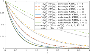
where Idd×dIdsuperscript𝑑𝑑\mathrm{Id}\in\mathbb{R}^{d\times d} is the identity matrix and diag:dd×d:diagsuperscript𝑑superscript𝑑𝑑\textrm{diag}:\mathbb{R}^{d}\rightarrow\mathbb{R}^{d\times d} the operator mapping a vector onto a diagonal matrix with the vector as its diagonal. The term’s scaling encourages in particular agents far from vα(ρ^tN)subscript𝑣𝛼superscriptsubscript^𝜌𝑡𝑁v_{\alpha}({\widehat{\rho}_{t}^{N}}) to explore larger regions. The coordinate-dependent scaling of anisotropic diffusion has proven to be particularly beneficial for high-dimensional optimization problems by yielding dimension-independent convergence rates (see Figure 1) and therefore improving both computational complexity and success probability of the algorithm [4, 7].

A theoretical convergence analysis of the CBO dynamics is possible either on the microscopic level (1) or by analyzing the macroscopic behavior of the particle density through a mean-field limit. In the large particle limit an agent is not influenced by individual particles but only by the average behavior of all particles. As shown in [11], the empirical random agent measure ρ^Nsuperscript^𝜌𝑁\widehat{\rho}^{N} converges in law to the deterministic agent density ρ𝒞([0,T],𝒫(d))𝜌𝒞0𝑇𝒫superscript𝑑\rho\in{\cal C}([0,T],{\cal P}(\mathbb{R}^{d})), which weakly (see Definition 1) satisfies the non-linear Fokker-Planck equation

tρt=λdiv((vvα(ρt))ρt)+σ22k=1dkk(D(Vtivα(ρ^tN))kk2ρt).subscript𝑡subscript𝜌𝑡𝜆div𝑣subscript𝑣𝛼subscript𝜌𝑡subscript𝜌𝑡superscript𝜎22superscriptsubscript𝑘1𝑑subscript𝑘𝑘𝐷superscriptsubscriptsuperscriptsubscript𝑉𝑡𝑖subscript𝑣𝛼superscriptsubscript^𝜌𝑡𝑁𝑘𝑘2subscript𝜌𝑡\displaystyle\partial_{t}\rho_{t}=\lambda\textrm{div}\big{(}\!\left(v-v_{\alpha}({\rho_{t}})\right)\rho_{t}\big{)}+\frac{\sigma^{2}}{2}\sum_{k=1}^{d}\partial_{kk}\left(D\!\left(V_{t}^{i}-v_{\alpha}({\widehat{\rho}_{t}^{N}})\right)_{kk}^{2}\rho_{t}\right). (2)

A quantitative analysis of the convergence rate remains, on non-compact domains, an open problem, see, e.g., [8, Remark 2]. Analyzing a mean-field limit such as (2) allows for establishing strong qualitative theoretical guarantees about CBO methods, paving the way to understand the internal mechanisms at play.

1.0.1 Prior Arts.

The original CBO work [16] proposes the dynamics (1) with isotropic diffusion, which is analyzed in the mean-field sense in [2]. Under a stringent well-preparedness condition about ρ0subscript𝜌0\rho_{0} and 𝒞2superscript𝒞2{\cal C}^{2} regularity of {\cal E} the authors show consensus formation of the particles at some v~~𝑣\widetilde{v} close to vsuperscript𝑣v^{*} by first establishing exponential decay of the variance Var(ρt)Varsubscript𝜌𝑡\operatorname{Var}\left({\rho_{t}}\right) and consecutively showing v~v~𝑣superscript𝑣\widetilde{v}\approx v^{*} as a consequence of the Laplace principle [15]. This analysis is extended to the anisotropic case in [4].

Motivated by the surprising phenomenon that, on average, individual agents of the CBO dynamics follow the gradient flow of vvv22maps-to𝑣superscriptsubscriptnorm𝑣superscript𝑣22v\!\mapsto\!\left\|{v-v^{*}}\right\|_{2}^{2}, see [8, Figure 1b], the authors of [8] develop a novel proof technique for showing global convergence of isotropic CBO in mean-field law to vsuperscript𝑣v^{*} under minimal assumptions. Following [8, Definition 1], we speak of convergence in mean-field law to vsuperscript𝑣v^{*} for the interacting particle dynamics (1), if the solution ρtsubscript𝜌𝑡\rho_{t} to the associated mean-field limit dynamics (2) converges narrowly to the Dirac delta δvsubscript𝛿superscript𝑣\delta_{v^{*}} at vsuperscript𝑣v^{*} for t𝑡t\rightarrow\infty. The proof is based on showing an exponential decay of the energy functional 𝒱:𝒫(d)0:𝒱𝒫superscript𝑑subscriptabsent0{\cal V}:{\cal P}(\mathbb{R}^{d})\!\rightarrow\!\mathbb{R}_{\geq 0}, given by

𝒱(ρt):=12vv22𝑑ρt(v).assign𝒱subscript𝜌𝑡12superscriptsubscriptnorm𝑣superscript𝑣22differential-dsubscript𝜌𝑡𝑣{\cal V}(\rho_{t}):=\frac{1}{2}\int\left\|{v-v^{*}}\right\|_{2}^{2}d\rho_{t}(v). (3)

This simultaneously ensures consensus formation and convergence of ρtsubscript𝜌𝑡\rho_{t} to δvsubscript𝛿superscript𝑣\delta_{v^{*}}.

1.0.2 Contribution.

In view of the effectiveness and efficiency of CBO methods with anisotropic diffusion for high-dimensional optimization problems, a thorough understanding is of considerable interest.
Refer to caption
(a) The Rastrigin function in one coordinate direction
Refer to caption
(b) Evolution of 𝒱(ρ^tN)𝒱superscriptsubscript^𝜌𝑡𝑁{\cal V}(\widehat{\rho}_{t}^{N}) for isotropic and anisotropic CBO for different dimensions
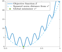
Figure 1: A demonstration of the benefit of using anisotropic diffusion in CBO. For the Rastrigin function (v)=k=1dvk2+52(1cos(2πvk))𝑣superscriptsubscript𝑘1𝑑superscriptsubscript𝑣𝑘25212𝜋subscript𝑣𝑘{\cal E}(v)\!=\!\sum_{k=1}^{d}\!v_{k}^{2}\!+\!\frac{5}{2}(1\!-\!\cos(2\pi v_{k})) with v=0superscript𝑣0v^{*}\!=\!0 and spurious local minima (see (a)), we evolve the discretized system of isotropic and anisotropic CBO using N=320000𝑁320000N=320000 agents, discrete time step size Δt=0.01Δ𝑡0.01\Delta t=0.01 and α=1015𝛼superscript1015\alpha=10^{15}, λ=1𝜆1\lambda=1, and σ=0.32𝜎0.32\sigma=0.32 for different dimensions d{4,8,12,16}𝑑481216d\in\{4,8,12,16\}.
We observe in (b) that the convergence rate of the energy functional 𝒱(ρ^tN)𝒱superscriptsubscript^𝜌𝑡𝑁{\cal V}(\widehat{\rho}_{t}^{N}) for isotropic CBO (dashed lines) is affected by the ambient dimension d𝑑d, whereas anisotropic CBO (solid lines) converges independently from d𝑑d with rate (2λσ2)2𝜆superscript𝜎2(2\lambda-\sigma^{2}).

As we illustrate in Figure 1, anisotropic CBO [4] converges with a dimension-independent rate as opposed to isotropic CBO [16, 2, 8], making it a particularly interesting choice for problems in high-dimensional spaces, e.g., from signal processing and machine learning applications. In this work we extend the analysis of [8] from isotropic CBO to CBO with anisotropic diffusion. More precisely, we show global convergence of the anisotropic CBO dynamics in mean-field law to the global minimizer vsuperscript𝑣v^{*} under minimal assumptions about the initial measure ρ0subscript𝜌0\rho_{0} and for a rich class of objectives {\cal E}. Furthermore, utilizing some tweaks in the implementation of anisotropic CBO, such as a random mini-batch idea and a cooling strategy of the parameters as proposed in [4, 9], we show that CBO performs well, in fact, almost on par with state-of-the-art gradient based methods, on a long-studied machine learning benchmark in 2000 dimensions, despite using just 1000 particles and no gradient information. This encourages the use and further investigation of CBO as a training algorithm for challenging machine learning tasks.

1.0.3 Organization.

In Section 2 we first recall details about the well-posedness of the mean-field dynamics (2) in the case of anisotropic diffusion before we present the main theoretical result about the convergence of anisotropic CBO in mean-field law. The proof then follows in Section 3. Section 4 illustrates the practicability of the optimization method on a benchmark problem and Section 5 concludes the paper. For the sake of reproducible research, in the GitHub repository https://github.com/KonstantinRiedl/CBOGlobalConvergenceAnalysis we provide the Matlab code implementing the CBO algorithm used in this work.

1.0.4 Notation.

Br(u)subscriptsuperscript𝐵𝑟𝑢B^{\infty}_{r}(u) is a closed superscript\ell^{\infty} ball in dsuperscript𝑑\mathbb{R}^{d} with center u𝑢u and radius r𝑟r. For the space of continuous functions f:XY:𝑓𝑋𝑌f:X\rightarrow Y we write 𝒞(X,Y)𝒞𝑋𝑌{\cal C}(X,Y), with Xn𝑋superscript𝑛X\subset\mathbb{R}^{n}, n𝑛n\in\mathbb{N}, and a suitable topological space Y𝑌Y. For Xn𝑋superscript𝑛X\subset\mathbb{R}^{n} open and for Y=m𝑌superscript𝑚Y=\mathbb{R}^{m}, m𝑚m\in\mathbb{N}, the function space 𝒞ck(X,Y)subscriptsuperscript𝒞𝑘𝑐𝑋𝑌{\cal C}^{k}_{c}(X,Y) contains functions f𝒞(X,Y)𝑓𝒞𝑋𝑌f\in{\cal C}(X,Y) that are k𝑘k-times continuously differentiable and compactly supported. Y𝑌Y is omitted if Y=𝑌Y=\mathbb{R}.

The objects of study are laws of stochastic processes, ρ𝒞([0,T],𝒫(d))𝜌𝒞0𝑇𝒫superscript𝑑\rho\in{\cal C}([0,T],{\cal P}(\mathbb{R}^{d})), where 𝒫(d)𝒫superscript𝑑{\cal P}(\mathbb{R}^{d}) contains all Borel probability measures over dsuperscript𝑑\mathbb{R}^{d}. ρt𝒫(d)subscript𝜌𝑡𝒫superscript𝑑\rho_{t}\in{\cal P}(\mathbb{R}^{d}) is a snapshot of such law at time t𝑡t and ϱitalic-ϱ\varrho some fixed distribution. Measures ϱ𝒫(d)italic-ϱ𝒫superscript𝑑\varrho\in{\cal P}(\mathbb{R}^{d}) with finite p𝑝p-th moment are collected in 𝒫p(d)subscript𝒫𝑝superscript𝑑{\cal P}_{p}(\mathbb{R}^{d}). For any 1p<1𝑝1\leq p<\infty, Wpsubscript𝑊𝑝W_{p} denotes the Wasserstein-p𝑝p distance. 𝔼(ϱ)𝔼italic-ϱ\mathbb{E}(\varrho) is the expectation of a probability measure ϱitalic-ϱ\varrho.

2 Global Convergence in Mean-Field Law

In this section we first recite a well-posedness result about the Fokker-Planck equation (2) and then present the main result about global convergence.

2.1 Definition of Weak Solutions and Well-Posedness

We begin by defining weak solutions of the Fokker-Planck equation (2).

Definition 1

Let ρ0𝒫(d)subscript𝜌0𝒫superscript𝑑\rho_{0}\in{\cal P}(\mathbb{R}^{d}), T>0𝑇0T>0. We say ρ𝒞([0,T],𝒫(d))𝜌𝒞0𝑇𝒫superscript𝑑\rho\in{\cal C}([0,T],{\cal P}(\mathbb{R}^{d})) satisfies the Fokker-Planck equation (2) with initial condition ρ0subscript𝜌0\rho_{0} in the weak sense in the time interval [0,T]0𝑇[0,T], if we have for all ϕ𝒞c(d)italic-ϕsuperscriptsubscript𝒞𝑐superscript𝑑\phi\in{\cal C}_{c}^{\infty}(\mathbb{R}^{d}) and all t(0,T)𝑡0𝑇t\in(0,T)

ddtϕ(v)𝑑ρt(v)=𝑑𝑑𝑡italic-ϕ𝑣differential-dsubscript𝜌𝑡𝑣absent\displaystyle\frac{d}{dt}\int\phi(v)\,d\rho_{t}(v)= λk=1d(vvα(ρt))kkϕ(v)dρt(v)𝜆superscriptsubscript𝑘1𝑑subscript𝑣subscript𝑣𝛼subscript𝜌𝑡𝑘subscript𝑘italic-ϕ𝑣𝑑subscript𝜌𝑡𝑣\displaystyle-\lambda\int\sum_{k=1}^{d}(v-v_{\alpha}({\rho_{t}}))_{k}\partial_{k}\phi(v)\,d\rho_{t}(v) (4)
+σ22k=1dD(Vtivα(ρ^tN))kk2kk2ϕ(v)dρt(v)superscript𝜎22superscriptsubscript𝑘1𝑑𝐷superscriptsubscriptsuperscriptsubscript𝑉𝑡𝑖subscript𝑣𝛼superscriptsubscript^𝜌𝑡𝑁𝑘𝑘2subscriptsuperscript2𝑘𝑘italic-ϕ𝑣𝑑subscript𝜌𝑡𝑣\displaystyle+\frac{\sigma^{2}}{2}\int\sum_{k=1}^{d}D\!\left(V_{t}^{i}-v_{\alpha}({\widehat{\rho}_{t}^{N}})\right)_{kk}^{2}\partial^{2}_{kk}\phi(v)\,d\rho_{t}(v)

and limt0ρt=ρ0subscript𝑡0subscript𝜌𝑡subscript𝜌0\lim_{t\rightarrow 0}\rho_{t}=\rho_{0} pointwise.

In what follows the case of CBO with anisotropic diffusion is considered, i.e., D(Vtivα(ρ^tN))=diag(Vtivα(ρ^tN))𝐷superscriptsubscript𝑉𝑡𝑖subscript𝑣𝛼superscriptsubscript^𝜌𝑡𝑁diagsuperscriptsubscript𝑉𝑡𝑖subscript𝑣𝛼superscriptsubscript^𝜌𝑡𝑁D\!\left(V_{t}^{i}-v_{\alpha}({\widehat{\rho}_{t}^{N}})\right)=\textrm{diag}\left(V_{t}^{i}-v_{\alpha}({\widehat{\rho}_{t}^{N}})\right) in Equations (1), (2) and (4).

Analogously to the well-posedness results [2, Theorems 3.1, 3.2] for CBO with isotropic diffusion, we can obtain well-posedness of (2) for anisotropic CBO.

Theorem 2.1

Let T>0𝑇0T>0, ρ0𝒫4(d)subscript𝜌0subscript𝒫4superscript𝑑\rho_{0}\in{\cal P}_{4}(\mathbb{R}^{d}) and consider :d:superscript𝑑{\cal E}:\mathbb{R}^{d}\rightarrow\mathbb{R} with ¯:=(v)>assign¯superscript𝑣\mkern 1.5mu\underline{\mkern-1.5mu{\cal E}\mkern-1.5mu}\mkern 1.5mu:={\cal E}(v^{*})>-\infty, which, for some constants C1,C2>0subscript𝐶1subscript𝐶20C_{1},C_{2}>0, satisfies

|(v)(w)|𝑣𝑤\displaystyle\left|{{\cal E}(v)-{\cal E}(w)}\right| C1(v2+w2)vw2,for all v,wd,formulae-sequenceabsentsubscript𝐶1subscriptnorm𝑣2subscriptnorm𝑤2subscriptnorm𝑣𝑤2for all 𝑣𝑤superscript𝑑\displaystyle\leq C_{1}(\left\|{v}\right\|_{2}+\left\|{w}\right\|_{2})\left\|{v-w}\right\|_{2},\quad\textrm{for all }v,w\in\mathbb{R}^{d},
(v)¯𝑣¯\displaystyle{\cal E}(v)-\mkern 1.5mu\underline{\mkern-1.5mu{\cal E}\mkern-1.5mu}\mkern 1.5mu C2(1+v22),for all vd.formulae-sequenceabsentsubscript𝐶21superscriptsubscriptnorm𝑣22for all 𝑣superscript𝑑\displaystyle\leq C_{2}\big{(}1+\left\|{v}\right\|_{2}^{2}\big{)},\quad\textrm{for all }v\in\mathbb{R}^{d}.

If in addition, either supvd(v)<subscriptsupremum𝑣superscript𝑑𝑣\sup_{v\in\mathbb{R}^{d}}{\cal E}(v)<\infty, or, for some C3,C4>0subscript𝐶3subscript𝐶40C_{3},C_{4}>0, {\cal E} satisfies

(v)¯C3v22,for all v2C4,formulae-sequence𝑣¯subscript𝐶3superscriptsubscriptnorm𝑣22for all subscriptnorm𝑣2subscript𝐶4\displaystyle{\cal E}(v)-\mkern 1.5mu\underline{\mkern-1.5mu{\cal E}\mkern-1.5mu}\mkern 1.5mu\geq C_{3}\left\|{v}\right\|_{2}^{2},\quad\textrm{for all }\left\|{v}\right\|_{2}\geq C_{4},

then there exists a law ρ𝒞([0,T],𝒫4(d))𝜌𝒞0𝑇subscript𝒫4superscript𝑑\rho\in{\cal C}([0,T],{\cal P}_{4}(\mathbb{R}^{d})) weakly satisfying Equation (2).

Proof

The proof follows the lines of the ones provided for [2, Theorems 3.1, 3.2].

Remark 1

As discussed in [8, Remark 7], the proof of Theorem 2.1 justifies an extension of the test function space 𝒞c(d)subscriptsuperscript𝒞𝑐superscript𝑑{\cal C}^{\infty}_{c}(\mathbb{R}^{d}) in Definition 1 to

𝒞2(d):={ϕ𝒞2(d):|kϕ(v)|c(1+|vk|) and kk2ϕ< for all k{1,,d} and some constant c>0}.assignsubscriptsuperscript𝒞2superscript𝑑conditional-setitalic-ϕsuperscript𝒞2superscript𝑑subscript𝑘italic-ϕ𝑣𝑐1subscript𝑣𝑘 and subscriptdelimited-∥∥subscriptsuperscript2𝑘𝑘italic-ϕ for all 𝑘1𝑑 and some constant 𝑐0\begin{split}{\cal C}^{2}_{*}(\mathbb{R}^{d}):=\big{\{}\phi\in{\cal C}^{2}(\mathbb{R}^{d}):&\left|{\partial_{k}\phi(v)}\right|\leq c(1+\left|{v_{k}}\right|)\text{ and }\|{\partial^{2}_{kk}\phi}\|_{\infty}<\infty\\ &\text{ for all }k\in\{1,\dots,d\}\text{ and some constant }c>0\big{\}}.\end{split}

2.2 Main Results

We now present the main result about global convergence in mean-field law for objective functions that satisfy the following conditions.

Definition 2 (Assumptions)

We consider functions 𝒞(d)𝒞superscript𝑑{\cal E}\in{\cal C}(\mathbb{R}^{d}), for which

  1. A1

    there exists vdsuperscript𝑣superscript𝑑v^{*}\in\mathbb{R}^{d} such that (v)=infvd(v)=:¯{\cal E}(v^{*})=\inf_{v\in\mathbb{R}^{d}}{\cal E}(v)=:\mkern 1.5mu\underline{\mkern-1.5mu{\cal E}\mkern-1.5mu}\mkern 1.5mu, and

  2. A2

    there exist ,R0,η>0subscriptsubscript𝑅0𝜂0{\cal E}_{\infty},R_{0},\eta>0, and ν(0,1/2]𝜈012\nu\in(0,1/2] such that

    vvsubscriptnorm𝑣superscript𝑣\displaystyle\|{v-v^{*}}\|_{\infty} 1η((v)¯)ν for all vBR0(v),formulae-sequenceabsent1𝜂superscript𝑣¯𝜈 for all 𝑣subscriptsuperscript𝐵subscript𝑅0superscript𝑣\displaystyle\leq\frac{1}{\eta}\big{(}{\cal E}(v)-\mkern 1.5mu\underline{\mkern-1.5mu{\cal E}\mkern-1.5mu}\mkern 1.5mu\big{)}^{\nu}\quad\textrm{ for all }v\in B^{\infty}_{R_{0}}(v^{*}), (5)
    subscript\displaystyle{\cal E}_{\infty} <(v)¯ for all v(BR0(v))c.formulae-sequenceabsent𝑣¯ for all 𝑣superscriptsubscriptsuperscript𝐵subscript𝑅0superscript𝑣𝑐\displaystyle<{\cal E}(v)-\mkern 1.5mu\underline{\mkern-1.5mu{\cal E}\mkern-1.5mu}\mkern 1.5mu\quad\textrm{ for all }v\in\big{(}B^{\infty}_{R_{0}}(v^{*})\big{)}^{c}. (6)

Assumption A2 can be regarded as a tractability condition of the energy landscape around the minimizer and in the farfield. Equation (5) requires the local coercivity of {\cal E}, whereas (6) prevents that (v)¯𝑣¯{\cal E}(v)\approx\mkern 1.5mu\underline{\mkern-1.5mu{\cal E}\mkern-1.5mu}\mkern 1.5mu far away from vsuperscript𝑣v^{*}.

Definition 2 covers a wide range of function classes, including for instance the Rastrigin function, see Figure 1(a), and objectives related to various machine learning tasks, see, e.g., [9].

For more detailed information we refer to the discussion after [8, Definition 9].

Theorem 2.2

Let {\cal E} be as in Definition 2. Moreover, let ρ0𝒫4(d)subscript𝜌0subscript𝒫4superscript𝑑\rho_{0}\in{\cal P}_{\!4}(\mathbb{R}^{d}) be such that

ρ0(Br(v))>0for allr>0.formulae-sequencesubscript𝜌0subscriptsuperscript𝐵𝑟superscript𝑣0for all𝑟0\displaystyle\rho_{0}(B^{\infty}_{r}(v^{*}))>0\quad\textrm{for all}\quad r>0. (7)

Define 𝒱(ρt):=1/2vv22𝑑ρt(v)assign𝒱subscript𝜌𝑡12superscriptsubscriptnorm𝑣superscript𝑣22differential-dsubscript𝜌𝑡𝑣{\cal V}(\rho_{t}):=1/2\int\left\|{v-v^{*}}\right\|_{2}^{2}d\rho_{t}(v). Fix any ε(0,𝒱(ρ0))𝜀0𝒱subscript𝜌0\varepsilon\in(0,{\cal V}(\rho_{0})) and τ(0,1)𝜏01\tau\in(0,1), parameters λ,σ>0𝜆𝜎0\lambda,\sigma>0 with 2λ>σ22𝜆superscript𝜎22\lambda>\sigma^{2}, and the time horizon

T:=1(1τ)(2λσ2)log(𝒱(ρ0)ε).assignsuperscript𝑇11𝜏2𝜆superscript𝜎2𝒱subscript𝜌0𝜀\displaystyle T^{*}:=\frac{1}{(1-\tau)\left(2\lambda-\sigma^{2}\right)}\log\left(\frac{{\cal V}(\rho_{0})}{\varepsilon}\right). (8)

Then there exists α0>0subscript𝛼00\alpha_{0}>0, which depends (among problem dependent quantities) on ε𝜀\varepsilon and τ𝜏\tau, such that for all α>α0𝛼subscript𝛼0\alpha>\alpha_{0}, if ρ𝒞([0,T],𝒫4(d))𝜌𝒞0superscript𝑇subscript𝒫4superscript𝑑\rho\in{\cal C}([0,T^{*}],{\cal P}_{4}(\mathbb{R}^{d})) is a weak solution to the Fokker-Planck equation (2) on the time interval [0,T]0superscript𝑇[0,T^{*}] with initial condition ρ0subscript𝜌0\rho_{0}, we have mint[0,T]𝒱(t)εsubscript𝑡0superscript𝑇𝒱𝑡𝜀\min_{t\in[0,T^{*}]}{\cal V}(t)\leq\varepsilon. Furthermore, until 𝒱(ρt)𝒱subscript𝜌𝑡{\cal V}(\rho_{t}) reaches the prescribed accuracy ε𝜀\varepsilon, we have the exponential decay

𝒱(ρt)𝒱(ρ0)exp((1τ)(2λσ2)t)𝒱subscript𝜌𝑡𝒱subscript𝜌01𝜏2𝜆superscript𝜎2𝑡{\cal V}(\rho_{t})\leq{\cal V}(\rho_{0})\exp\left(-(1-\tau)\left(2\lambda-\sigma^{2}\right)t\right)

and, up to a constant, the same behavior for W22(ρt,δv)superscriptsubscript𝑊22subscript𝜌𝑡subscript𝛿superscript𝑣W_{2}^{2}(\rho_{t},\delta_{v^{*}}).

The rate of convergence (2λσ2)2𝜆superscript𝜎2(2\lambda-\sigma^{2}) obtained in Theorem 2.2 is confirmed numerically by the experiments depicted in Figure 1. We emphasize the dimension-independent convergence of CBO with anisotropic diffusion, contrasting the dimension-dependent rate (2λdσ2)2𝜆𝑑superscript𝜎2(2\lambda-d\sigma^{2}) of isotropic CBO, cf. [8, Theorem 12].

3 Proof of Theorem 2.2

This section provides the proof details for Theorem 2.2, starting with a sketch in Section 3.1. Sections 3.23.4 present statements, which are needed in the proof and may be of independent interest. Section 3.5 completes the proof.

Remark 2

Without loss of generality we assume ¯=0¯0\mkern 1.5mu\underline{\mkern-1.5mu{\cal E}\mkern-1.5mu}\mkern 1.5mu=0 throughout the proof.

3.1 Proof Sketch

The main idea is to show that 𝒱(ρt)𝒱subscript𝜌𝑡{\cal V}(\rho_{t}) satisfies the differential inequality

ddt𝒱(ρt)(1τ)(2λσ2)𝒱(ρt)𝑑𝑑𝑡𝒱subscript𝜌𝑡1𝜏2𝜆superscript𝜎2𝒱subscript𝜌𝑡\displaystyle\frac{d}{dt}{\cal V}(\rho_{t})\leq-(1-\tau)\left(2\lambda-\sigma^{2}\right){\cal V}(\rho_{t}) (9)

until 𝒱(ρT)ε𝒱subscript𝜌𝑇𝜀{\cal V}(\rho_{T})\leq\varepsilon. The first step towards (9) is to derive a differential inequality for 𝒱(ρt)𝒱subscript𝜌𝑡{\cal V}(\rho_{t}) using the dynamics of ρ𝜌\rho, which is done in Lemma 1. In order to control the appearing quantity vα(ρt)v2subscriptnormsubscript𝑣𝛼subscript𝜌𝑡superscript𝑣2\left\|{v_{\alpha}({\rho_{t}})-v^{*}}\right\|_{2}, we establish a quantitative Laplace principle. Namely, under the inverse continuity property A2, Proposition 1 shows

vα(ρt)v2(r)+dexp(αr)ρt(Br(v)),for sufficiently small r>0,formulae-sequenceless-than-or-similar-tosubscriptnormsubscript𝑣𝛼subscript𝜌𝑡superscript𝑣2𝑟𝑑𝛼𝑟subscript𝜌𝑡subscriptsuperscript𝐵𝑟superscript𝑣for sufficiently small 𝑟0\displaystyle\left\|{v_{\alpha}({\rho_{t}})-v^{*}}\right\|_{2}\lesssim\ell(r)+\frac{\sqrt{d}\exp(-\alpha r)}{\rho_{t}(B^{\infty}_{r}(v^{*}))},\quad\textrm{for sufficiently small }r>0,

where \ell is decreasing with (r)0+𝑟superscript0\ell(r)\rightarrow 0^{+} as r0𝑟0r\rightarrow 0. Thus, vα(ρt)v2subscriptnormsubscript𝑣𝛼subscript𝜌𝑡superscript𝑣2\left\|{v_{\alpha}({\rho_{t}})-v^{*}}\right\|_{2} can be made arbitrarily small by suitable choices of r1much-less-than𝑟1r\ll 1 and α1much-greater-than𝛼1\alpha\gg 1, as long as we can guarantee ρt(Br(v))>0subscript𝜌𝑡subscriptsuperscript𝐵𝑟superscript𝑣0\rho_{t}(B^{\infty}_{r}(v^{*}))>0 for all r>0𝑟0r>0 and at all times t[0,T]𝑡0𝑇t\in[0,T]. The latter requires non-zero initial mass ρ0(Br(v))subscript𝜌0subscriptsuperscript𝐵𝑟superscript𝑣\rho_{0}(B^{\infty}_{r}(v^{*})) as well as an active Brownian motion, as made rigorous in Proposition 2.

3.2 Evolution of the Mean-Field Limit

We now derive the evolution inequality of the energy functional 𝒱(ρt)𝒱subscript𝜌𝑡{\cal V}(\rho_{t}).

Lemma 1

Let :d:superscript𝑑{\cal E}:\mathbb{R}^{d}\rightarrow\mathbb{R}, and fix α,λ,σ>0𝛼𝜆𝜎0\alpha,\lambda,\sigma>0. Moreover, let T>0𝑇0T>0 and let ρ𝒞([0,T],𝒫4(d))𝜌𝒞0𝑇subscript𝒫4superscript𝑑\rho\in{\cal C}([0,T],{\cal P}_{4}(\mathbb{R}^{d})) be a weak solution to Equation (2). Then 𝒱(ρt)𝒱subscript𝜌𝑡{\cal V}(\rho_{t}) satisfies

ddt𝒱(ρt)𝑑𝑑𝑡𝒱subscript𝜌𝑡absent\displaystyle\frac{d}{dt}{\cal V}(\rho_{t})\leq (2λσ2)𝒱(ρt)+2(λ+σ2)𝒱(ρt)vα(ρt)v22𝜆superscript𝜎2𝒱subscript𝜌𝑡2𝜆superscript𝜎2𝒱subscript𝜌𝑡subscriptnormsubscript𝑣𝛼subscript𝜌𝑡superscript𝑣2\displaystyle\,-\left(2\lambda-\sigma^{2}\right){\cal V}(\rho_{t})+\sqrt{2}\left(\lambda+\sigma^{2}\right)\sqrt{{\cal V}(\rho_{t})}\left\|{v_{\alpha}({\rho_{t}})-v^{*}}\right\|_{2}
+σ22vα(ρt)v22.superscript𝜎22superscriptsubscriptnormsubscript𝑣𝛼subscript𝜌𝑡superscript𝑣22\displaystyle\,+\frac{\sigma^{2}}{2}\left\|{v_{\alpha}({\rho_{t}})-v^{*}}\right\|_{2}^{2}.
Proof

Noting that ϕ(v)=1/2vv22italic-ϕ𝑣12superscriptsubscriptnorm𝑣superscript𝑣22\phi(v)=1/2\left\|{v-v^{*}}\right\|_{2}^{2} is in 𝒞2(d)superscriptsubscript𝒞2superscript𝑑{\cal C}_{*}^{2}(\mathbb{R}^{d}) and recalling that ρ𝜌\rho satisfies the identity (4) for all test functions in 𝒞2(d)superscriptsubscript𝒞2superscript𝑑{\cal C}_{*}^{2}(\mathbb{R}^{d}), see Remark 1, we obtain

ddt𝒱(ρt)=λvv,vvα(ρt)𝑑ρt(v)+σ22vvα(ρt)22𝑑ρt(v),𝑑𝑑𝑡𝒱subscript𝜌𝑡𝜆𝑣superscript𝑣𝑣subscript𝑣𝛼subscript𝜌𝑡differential-dsubscript𝜌𝑡𝑣superscript𝜎22superscriptsubscriptnorm𝑣subscript𝑣𝛼subscript𝜌𝑡22differential-dsubscript𝜌𝑡𝑣\displaystyle\frac{d}{dt}{\cal V}(\rho_{t})=-\lambda\int\langle v-v^{*},v-v_{\alpha}({\rho_{t}})\rangle\,d\rho_{t}(v)+\frac{\sigma^{2}}{2}\int\left\|{v-v_{\alpha}({\rho_{t}})}\right\|_{2}^{2}d\rho_{t}(v),

where we used kϕ(v)=(vv)ksubscript𝑘italic-ϕ𝑣subscript𝑣superscript𝑣𝑘\partial_{k}\phi(v)=\left(v-v^{*}\right)_{k} and kk2ϕ(v)=1subscriptsuperscript2𝑘𝑘italic-ϕ𝑣1\partial^{2}_{kk}\phi(v)=1 for all k{1,,d}𝑘1𝑑k\in\{1,\dots,d\}. Following the steps taken in [8, Lemma 14] yields the statement. \square

3.3 Quantitative Laplace Principle

The Laplace principle asserts that log(ωαL1(ϱ))/α¯subscriptnormsubscript𝜔𝛼subscript𝐿1italic-ϱ𝛼¯-\log(\|{\omega_{\alpha}}\|_{L_{1}(\varrho)})/\alpha\rightarrow\mkern 1.5mu\underline{\mkern-1.5mu{\cal E}\mkern-1.5mu}\mkern 1.5mu as α𝛼\alpha\rightarrow\infty as long as the global minimizer vsuperscript𝑣v^{*} is in the support of ϱitalic-ϱ\varrho. Under the assumption of the inverse continuity property this can be used to qualitatively characterize the proximity of vα(ϱ)subscript𝑣𝛼italic-ϱv_{\alpha}({\varrho}) to the global minimizer vsuperscript𝑣v^{*}. However, as it neither allows to quantify this proximity nor gives a suggestion on how to choose α𝛼\alpha to reach a certain approximation quality, we introduced a quantitative version in [8, Proposition 17], which we now adapt suitably to satisfy the anisotropic setting.

Proposition 1

Let ¯=0¯0\mkern 1.5mu\underline{\mkern-1.5mu{\cal E}\mkern-1.5mu}\mkern 1.5mu=0, ϱ𝒫(d)italic-ϱ𝒫superscript𝑑\varrho\in{\cal P}(\mathbb{R}^{d}) and fix α>0𝛼0\alpha>0. For any r>0𝑟0r>0 we define r:=supvBr(v)(v)assignsubscript𝑟subscriptsupremum𝑣subscriptsuperscript𝐵𝑟superscript𝑣𝑣{\cal E}_{r}:=\sup_{v\in B^{\infty}_{r}(v^{*})}{\cal E}(v). Then, under the inverse continuity property A2, for any r(0,R0]𝑟0subscript𝑅0r\in(0,R_{0}] and q>0𝑞0q>0 such that q+r𝑞subscript𝑟subscriptq+{\cal E}_{r}\leq{\cal E}_{\infty}, we have

vα(ϱ)v2d(q+r)νη+dexp(αq)ϱ(Br(v))vv2𝑑ϱ(v).subscriptnormsubscript𝑣𝛼italic-ϱsuperscript𝑣2𝑑superscript𝑞subscript𝑟𝜈𝜂𝑑𝛼𝑞italic-ϱsubscriptsuperscript𝐵𝑟superscript𝑣subscriptnorm𝑣superscript𝑣2differential-ditalic-ϱ𝑣\displaystyle\left\|{v_{\alpha}({\varrho})-v^{*}}\right\|_{2}\leq\frac{\sqrt{d}(q+{\cal E}_{r})^{\nu}}{\eta}+\frac{\sqrt{d}\exp(-\alpha q)}{\varrho(B^{\infty}_{r}(v^{*}))}\int\left\|{v-v^{*}}\right\|_{2}d\varrho(v).
Proof

Following the lines of the proof of [8, Proposition 17] but replacing all 2superscript2\ell^{2} balls and norms by superscript\ell^{\infty} balls and norms, respectively, we obtain

vα(ϱ)v(q+r)νη+exp(αq)ϱ(Br(v))vv𝑑ϱ(v).subscriptnormsubscript𝑣𝛼italic-ϱsuperscript𝑣superscript𝑞subscript𝑟𝜈𝜂𝛼𝑞italic-ϱsubscriptsuperscript𝐵𝑟superscript𝑣subscriptnorm𝑣superscript𝑣differential-ditalic-ϱ𝑣\displaystyle\left\|{v_{\alpha}({\varrho})-v^{*}}\right\|_{\infty}\leq\frac{(q+{\cal E}_{r})^{\nu}}{\eta}+\frac{\exp\left(-\alpha q\right)}{\varrho(B^{\infty}_{r}(v^{*}))}\int\left\|{v-v^{*}}\right\|_{\infty}d\varrho(v).

The statement now follows noting that 2d\left\|{\cdot}\right\|_{\infty}\leq\left\|{\cdot}\right\|_{2}\leq\sqrt{d}\left\|{\cdot}\right\|_{\infty}. \square

3.4 A Lower Bound for the Probability Mass around vsuperscript𝑣v^{*}

In this section we provide a lower bound for the probability mass of ρt(Br(v))subscript𝜌𝑡subscriptsuperscript𝐵𝑟superscript𝑣\rho_{t}(B^{\infty}_{r}(v^{*})), where r>0𝑟0r>0 is a small radius. This is achieved by defining a mollifier ϕrsubscriptitalic-ϕ𝑟\phi_{r} so that ρt(Br(v))ϕr(v)𝑑ρt(v)subscript𝜌𝑡subscriptsuperscript𝐵𝑟superscript𝑣subscriptitalic-ϕ𝑟𝑣differential-dsubscript𝜌𝑡𝑣\rho_{t}(B^{\infty}_{r}(v^{*}))\geq\int\phi_{r}(v)\,d\rho_{t}(v) and studying the evolution of the right-hand side.

Lemma 2

For r>0𝑟0r>0 we define the mollifier ϕr:d:subscriptitalic-ϕ𝑟superscript𝑑\phi_{r}:\mathbb{R}^{d}\rightarrow\mathbb{R} by

ϕr(v):={k=1dexp(1r2r2(vv)k2), if vv<r,0, else.assignsubscriptitalic-ϕ𝑟𝑣casessuperscriptsubscriptproduct𝑘1𝑑1superscript𝑟2superscript𝑟2superscriptsubscript𝑣superscript𝑣𝑘2 if subscriptnorm𝑣superscript𝑣𝑟0 else.\displaystyle\phi_{r}(v):=\begin{cases}\prod_{k=1}^{d}\exp\left(1-\frac{r^{2}}{r^{2}-\left(v-v^{*}\right)_{k}^{2}}\right),&\textrm{ if }\left\|{v-v^{*}}\right\|_{\infty}<r,\\ 0,&\textrm{ else.}\end{cases} (10)

We have Im(ϕr)=[0,1]Imsubscriptitalic-ϕ𝑟01\operatorname{Im}(\phi_{r})=[0,1], supp(ϕr)=Br(v)suppsubscriptitalic-ϕ𝑟subscriptsuperscript𝐵𝑟superscript𝑣\operatorname{supp}(\phi_{r})=B^{\infty}_{r}(v^{*}), ϕr𝒞c(d)subscriptitalic-ϕ𝑟superscriptsubscript𝒞𝑐superscript𝑑\phi_{r}\in{\cal C}_{c}^{\infty}(\mathbb{R}^{d}) and

kϕr(v)subscript𝑘subscriptitalic-ϕ𝑟𝑣\displaystyle\partial_{k}\phi_{r}(v) =2r2(vv)k(r2(vv)k2)2ϕr(v),absent2superscript𝑟2subscript𝑣superscript𝑣𝑘superscriptsuperscript𝑟2subscriptsuperscript𝑣superscript𝑣2𝑘2subscriptitalic-ϕ𝑟𝑣\displaystyle=-2r^{2}\frac{\left(v-v^{*}\right)_{k}}{\left(r^{2}-\left(v-v^{*}\right)^{2}_{k}\right)^{2}}\phi_{r}(v),
kk2ϕr(v)subscriptsuperscript2𝑘𝑘subscriptitalic-ϕ𝑟𝑣\displaystyle\partial^{2}_{kk}\phi_{r}(v) =2r2(2(2(vv)k2r2)(vv)k2(r2(vv)k2)2(r2(vv)k2)4)ϕr(v).absent2superscript𝑟222subscriptsuperscript𝑣superscript𝑣2𝑘superscript𝑟2superscriptsubscript𝑣superscript𝑣𝑘2superscriptsuperscript𝑟2subscriptsuperscript𝑣superscript𝑣2𝑘2superscriptsuperscript𝑟2subscriptsuperscript𝑣superscript𝑣2𝑘4subscriptitalic-ϕ𝑟𝑣\displaystyle=2r^{2}\left(\frac{2\left(2\left(v-v^{*}\right)^{2}_{k}-r^{2}\right)\left(v-v^{*}\right)_{k}^{2}-\left(r^{2}-\left(v-v^{*}\right)^{2}_{k}\right)^{2}}{\left(r^{2}-\left(v-v^{*}\right)^{2}_{k}\right)^{4}}\right)\phi_{r}(v).
Proof

ϕrsubscriptitalic-ϕ𝑟\phi_{r} is a tensor product of classical well-studied mollifiers. \square

Proposition 2

Let T>0𝑇0T>0, r>0𝑟0r>0, and fix parameters α,λ,σ>0𝛼𝜆𝜎0\alpha,\lambda,\sigma>0. Assume ρ𝒞([0,T],𝒫(d))𝜌𝒞0𝑇𝒫superscript𝑑\rho\in{\cal C}([0,T],{\cal P}(\mathbb{R}^{d})) weakly solves the Fokker-Planck equation (2) in the sense of Definition 1 with initial condition ρ0𝒫(d)subscript𝜌0𝒫superscript𝑑\rho_{0}\in{\cal P}(\mathbb{R}^{d}) and for t[0,T]𝑡0𝑇t\in[0,T]. Furthermore, denote B:=supt[0,T]vα(ρt)vassign𝐵subscriptsupremum𝑡0𝑇subscriptnormsubscript𝑣𝛼subscript𝜌𝑡superscript𝑣B:=\sup_{t\in[0,T]}\left\|{v_{\alpha}({\rho_{t}})-v^{*}}\right\|_{\infty}. Then, for all t[0,T]𝑡0𝑇t\in[0,T] we have

ρt(Br(v))(ϕr(v)𝑑ρ0(v))exp(qt),forq:=2dmax{λ(cr+Bc)(1c)2r+σ2(cr2+B2)(2c+1)(1c)4r2,2λ2(2c1)σ2},subscript𝜌𝑡subscriptsuperscript𝐵𝑟superscript𝑣absentsubscriptitalic-ϕ𝑟𝑣differential-dsubscript𝜌0𝑣𝑞𝑡for𝑞assignabsent2𝑑𝜆𝑐𝑟𝐵𝑐superscript1𝑐2𝑟superscript𝜎2𝑐superscript𝑟2superscript𝐵22𝑐1superscript1𝑐4superscript𝑟22superscript𝜆22𝑐1superscript𝜎2\displaystyle\begin{aligned} \rho_{t}\left(B^{\infty}_{r}(v^{*})\right)&\geq\left(\int\phi_{r}(v)\,d\rho_{0}(v)\right)\exp\left(-qt\right),\\ \qquad\textrm{for}\quad q&:=2d\max\left\{\frac{\lambda(cr\!+\!B\sqrt{c})}{(1\!-\!c)^{2}r}\!+\!\frac{\sigma^{2}(cr^{2}\!+\!B^{2})(2c\!+\!1)}{(1\!-\!c)^{4}r^{2}},\frac{2\lambda^{2}}{(2c\!-\!1)\sigma^{2}}\right\}\!,\end{aligned} (11)

where c(1/2,1)𝑐121c\in(1/2,1) can be any constant that satisfies (1c)2(2c1)csuperscript1𝑐22𝑐1𝑐(1-c)^{2}\leq(2c-1)c.

Remark 3

In order to ensure a finite decay rate q<𝑞q<\infty in Proposition 2 it is crucial to have a non-vanishing diffusion σ>0𝜎0\sigma>0.

Proof (Proposition 2)

By the properties of the mollifier in Lemma 2 we have

ρt(Br(v))ϕr(v)𝑑ρt(v).subscript𝜌𝑡subscriptsuperscript𝐵𝑟superscript𝑣subscriptitalic-ϕ𝑟𝑣differential-dsubscript𝜌𝑡𝑣\displaystyle\rho_{t}\left(B^{\infty}_{r}(v^{*})\right)\geq\int\phi_{r}(v)\,d\rho_{t}(v).

Our strategy is to derive a lower bound for the right-hand side of this inequality. Using the weak solution property of ρ𝜌\rho and the fact that ϕr𝒞c(d)subscriptitalic-ϕ𝑟subscriptsuperscript𝒞𝑐superscript𝑑\phi_{r}\in{\cal C}^{\infty}_{c}(\mathbb{R}^{d}), we obtain

ddtϕr(v)𝑑ρt(v)𝑑𝑑𝑡subscriptitalic-ϕ𝑟𝑣differential-dsubscript𝜌𝑡𝑣\displaystyle\frac{d}{dt}\int\phi_{r}(v)\,d\rho_{t}(v) =k=1d(T1k(v)+T2k(v))𝑑ρt(v)absentsuperscriptsubscript𝑘1𝑑subscript𝑇1𝑘𝑣subscript𝑇2𝑘𝑣differential-dsubscript𝜌𝑡𝑣\displaystyle=\sum_{k=1}^{d}\int\big{(}T_{1k}(v)+T_{2k}(v)\big{)}\,d\rho_{t}(v) (12)
withT1k(v)withsubscript𝑇1𝑘𝑣\displaystyle\textrm{with}\quad T_{1k}(v) :=λ(vvα(ρt))kkϕr(v)assignabsent𝜆subscript𝑣subscript𝑣𝛼subscript𝜌𝑡𝑘subscript𝑘subscriptitalic-ϕ𝑟𝑣\displaystyle:=-\lambda\left(v-v_{\alpha}({\rho_{t}})\right)_{k}\partial_{k}\phi_{r}(v)
andT2k(v)andsubscript𝑇2𝑘𝑣\displaystyle\textrm{and}\quad T_{2k}(v) :=σ22(vvα(ρt))k2kk2ϕr(v)assignabsentsuperscript𝜎22superscriptsubscript𝑣subscript𝑣𝛼subscript𝜌𝑡𝑘2subscriptsuperscript2𝑘𝑘subscriptitalic-ϕ𝑟𝑣\displaystyle:=\frac{\sigma^{2}}{2}\left(v-v_{\alpha}({\rho_{t}})\right)_{k}^{2}\partial^{2}_{kk}\phi_{r}(v)

for k{1,,d}𝑘1𝑑k\in\{1,\dots,d\}. We now aim for showing T1k(v)+T2k(v)qϕr(v)subscript𝑇1𝑘𝑣subscript𝑇2𝑘𝑣𝑞subscriptitalic-ϕ𝑟𝑣T_{1k}(v)+T_{2k}(v)\geq-q\phi_{r}(v) uniformly on dsuperscript𝑑\mathbb{R}^{d} individually for each k𝑘k and for q>0𝑞0q>0 as in the statement. Since the mollifier ϕrsubscriptitalic-ϕ𝑟\phi_{r} and its derivatives vanish outside of Ωr:={vd:vv<r}assignsubscriptΩ𝑟conditional-set𝑣superscript𝑑subscriptnorm𝑣superscript𝑣𝑟\Omega_{r}:=\{v\in\mathbb{R}^{d}:\left\|{v-v^{*}}\right\|_{\infty}<r\} we restrict our attention to the open superscript\ell^{\infty}-ball ΩrsubscriptΩ𝑟\Omega_{r}. To achieve the lower bound over ΩrsubscriptΩ𝑟\Omega_{r}, we introduce for each k{1,,d}𝑘1𝑑k\in\{1,\dots,d\} the subsets

K1ksubscript𝐾1𝑘\displaystyle K_{1k} :={vd:|(vv)k|>cr}assignabsentconditional-set𝑣superscript𝑑subscript𝑣superscript𝑣𝑘𝑐𝑟\displaystyle:=\left\{v\in\mathbb{R}^{d}:\left|{\left(v-v^{*}\right)_{k}}\right|>\sqrt{c}r\right\} (13)

and

K2k:={vd:λ(vvα(ρt))k(vv)k(r2(vv)k2)2>c~r2σ22(vvα(ρt))k2(vv)k2},\displaystyle\begin{aligned} &K_{2k}:=\bigg{\{}v\in\mathbb{R}^{d}:-\lambda\left(v-v_{\alpha}({\rho_{t}})\right)_{k}\left(v-v^{*}\right)_{k}\left(r^{2}-\left(v-v^{*}\right)_{k}^{2}\right)^{2}\\ &\qquad\qquad\qquad\qquad\qquad\quad>\tilde{c}r^{2}\frac{\sigma^{2}}{2}\left(v-v_{\alpha}({\rho_{t}})\right)_{k}^{2}\left(v-v^{*}\right)_{k}^{2}\bigg{\}},\end{aligned} (14)

where c~:=2c1(0,1)assign~𝑐2𝑐101\tilde{c}:=2c-1\in(0,1). For fixed k𝑘k we now decompose ΩrsubscriptΩ𝑟\Omega_{r} according to

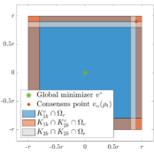
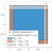
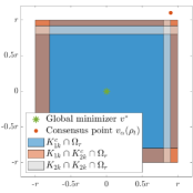
Ωr=(K1kcΩr)(K1kK2kcΩr)(K1kK2kΩr),subscriptΩ𝑟superscriptsubscript𝐾1𝑘𝑐subscriptΩ𝑟subscript𝐾1𝑘superscriptsubscript𝐾2𝑘𝑐subscriptΩ𝑟subscript𝐾1𝑘subscript𝐾2𝑘subscriptΩ𝑟\displaystyle\Omega_{r}=\left(K_{1k}^{c}\cap\Omega_{r}\right)\cup\left(K_{1k}\cap K_{2k}^{c}\cap\Omega_{r}\right)\cup\left(K_{1k}\cap K_{2k}\cap\Omega_{r}\right), (15)

which is illustrated in Figure 2 for different positions of vα(ρt)subscript𝑣𝛼subscript𝜌𝑡v_{\alpha}({\rho_{t}}) and values of σ𝜎\sigma.

Refer to caption
(a) vα(ρt)Ωrsubscript𝑣𝛼subscript𝜌𝑡subscriptΩ𝑟v_{\alpha}({\rho_{t}})\in\Omega_{r}, σ=0.2𝜎0.2\sigma=0.2
Refer to caption
(b) vα(ρt)Ωrsubscript𝑣𝛼subscript𝜌𝑡subscriptΩ𝑟v_{\alpha}({\rho_{t}})\not\in\Omega_{r}, σ=0.2𝜎0.2\sigma=0.2
Refer to caption
(c) vα(ρt)Ωrsubscript𝑣𝛼subscript𝜌𝑡subscriptΩ𝑟v_{\alpha}({\rho_{t}})\not\in\Omega_{r}, σ=1𝜎1\sigma=1
Figure 2: Visualization of the decomposition of ΩrsubscriptΩ𝑟\Omega_{r} as in (15) for different positions of vα(ρt)subscript𝑣𝛼subscript𝜌𝑡v_{\alpha}({\rho_{t}}) and values of σ𝜎\sigma.

In the following we treat each of these three subsets separately.

Subset K1kcΩrsuperscriptsubscript𝐾1𝑘𝑐subscriptΩ𝑟K_{1k}^{c}\cap\Omega_{r}: We have |(vv)k|crsubscript𝑣superscript𝑣𝑘𝑐𝑟\left|{\left(v-v^{*}\right)_{k}}\right|\leq\sqrt{c}r for each vK1kc𝑣superscriptsubscript𝐾1𝑘𝑐v\in K_{1k}^{c}, which can be used to independently derive lower bounds for both terms T1ksubscript𝑇1𝑘T_{1k} and T2ksubscript𝑇2𝑘T_{2k}. For T1ksubscript𝑇1𝑘T_{1k}, we insert the expression for kϕrsubscript𝑘subscriptitalic-ϕ𝑟\partial_{k}\phi_{r} from Lemma 2 to get

T1k(v)subscript𝑇1𝑘𝑣\displaystyle T_{1k}(v) =2r2λ(vvα(ρt))k(vv)k(r2(vv)k2)2ϕr(v)absent2superscript𝑟2𝜆subscript𝑣subscript𝑣𝛼subscript𝜌𝑡𝑘subscript𝑣superscript𝑣𝑘superscriptsuperscript𝑟2subscriptsuperscript𝑣superscript𝑣2𝑘2subscriptitalic-ϕ𝑟𝑣\displaystyle=2r^{2}\lambda\left(v-v_{\alpha}({\rho_{t}})\right)_{k}\frac{\left(v-v^{*}\right)_{k}}{\left(r^{2}-\left(v-v^{*}\right)^{2}_{k}\right)^{2}}\phi_{r}(v)
2r2λ|(vvα(ρt))k||(vv)k|(r2(vv)k2)2ϕr(v)2λ(cr+B)c(1c)2rϕr(v)absent2superscript𝑟2𝜆subscript𝑣subscript𝑣𝛼subscript𝜌𝑡𝑘subscript𝑣superscript𝑣𝑘superscriptsuperscript𝑟2subscriptsuperscript𝑣superscript𝑣2𝑘2subscriptitalic-ϕ𝑟𝑣2𝜆𝑐𝑟𝐵𝑐superscript1𝑐2𝑟subscriptitalic-ϕ𝑟𝑣\displaystyle\geq-2r^{2}\!\lambda\frac{\left|{\left(v-v_{\alpha}({\rho_{t}})\right)_{k}}\right|\!\left|{\left(v-v^{*}\right)_{k}}\right|}{\left(r^{2}-\left(v-v^{*}\right)^{2}_{k}\right)^{2}}\phi_{r}(v)\geq-\frac{2\lambda(\sqrt{c}r+B)\sqrt{c}}{(1-c)^{2}r}\phi_{r}(v)
=:q1ϕr(v),\displaystyle=:-q_{1}\phi_{r}(v),

where |(vvα(ρt))k||(vv)k|+|(vvα(ρt))k|cr+Bsubscript𝑣subscript𝑣𝛼subscript𝜌𝑡𝑘subscript𝑣superscript𝑣𝑘subscriptsuperscript𝑣subscript𝑣𝛼subscript𝜌𝑡𝑘𝑐𝑟𝐵\left|{(v-v_{\alpha}({\rho_{t}}))_{k}}\right|\leq\left|{(v-v^{*})_{k}}\right|+\left|{(v^{*}-v_{\alpha}({\rho_{t}}))_{k}}\right|\leq\sqrt{c}r+B is used in the last inequality. For T2subscript𝑇2T_{2} we insert the expression for kk2ϕrsubscriptsuperscript2𝑘𝑘subscriptitalic-ϕ𝑟\partial^{2}_{kk}\phi_{r} from Lemma 2 to obtain

T2k(v)subscript𝑇2𝑘𝑣\displaystyle T_{2k}(v) =σ2r2(vvα(ρt))k22(2(vv)k2r2)(vv)k2(r2(vv)k2)2(r2(vv)k2)4ϕr(v)absentsuperscript𝜎2superscript𝑟2superscriptsubscript𝑣subscript𝑣𝛼subscript𝜌𝑡𝑘222subscriptsuperscript𝑣superscript𝑣2𝑘superscript𝑟2superscriptsubscript𝑣superscript𝑣𝑘2superscriptsuperscript𝑟2subscriptsuperscript𝑣superscript𝑣2𝑘2superscriptsuperscript𝑟2subscriptsuperscript𝑣superscript𝑣2𝑘4subscriptitalic-ϕ𝑟𝑣\displaystyle=\sigma^{2}r^{2}\left(v\!-\!v_{\alpha}({\rho_{t}})\right)_{k}^{2}\frac{2\left(2\left(v\!-\!v^{*}\right)^{2}_{k}\!-\!r^{2}\right)\left(v\!-\!v^{*}\right)_{k}^{2}\!-\!\left(r^{2}\!-\!\left(v\!-\!v^{*}\right)^{2}_{k}\right)^{2}}{\left(r^{2}\!-\!\left(v\!-\!v^{*}\right)^{2}_{k}\right)^{4}}\phi_{r}(v)
2σ2(cr2+B2)(2c+1)(1c)4r2ϕr(v)=:q2ϕr(v),\displaystyle\geq-\frac{2\sigma^{2}(cr^{2}\!+\!B^{2})(2c\!+\!1)}{(1\!-\!c)^{4}r^{2}}\phi_{r}(v)=:-q_{2}\phi_{r}(v),

where the last inequality uses (vvα(ρt))k2(cr+B)22(cr2+B2)superscriptsubscript𝑣subscript𝑣𝛼subscript𝜌𝑡𝑘2superscript𝑐𝑟𝐵22𝑐superscript𝑟2superscript𝐵2(v-v_{\alpha}({\rho_{t}}))_{k}^{2}\leq\left(\sqrt{c}r+B\right)^{2}\leq 2(cr^{2}+B^{2}).

Subset K1kK2kcΩrsubscript𝐾1𝑘superscriptsubscript𝐾2𝑘𝑐subscriptΩ𝑟K_{1k}\cap K_{2k}^{c}\cap\Omega_{r}: As vK1k𝑣subscript𝐾1𝑘v\in K_{1k} we have |(vv)k|2>crsubscriptsubscript𝑣superscript𝑣𝑘2𝑐𝑟\left|{\left(v-v^{*}\right)_{k}}\right|_{2}>\sqrt{c}r. We observe that T1k(v)+T2k(v)0subscript𝑇1𝑘𝑣subscript𝑇2𝑘𝑣0T_{1k}(v)+T_{2k}(v)\geq 0 for all v𝑣v in this subset whenever

(λ(vvα(ρt))k(vv)k+σ22(vvα(ρt))k2)(r2(vv)k2)2𝜆subscript𝑣subscript𝑣𝛼subscript𝜌𝑡𝑘subscript𝑣superscript𝑣𝑘superscript𝜎22superscriptsubscript𝑣subscript𝑣𝛼subscript𝜌𝑡𝑘2superscriptsuperscript𝑟2subscriptsuperscript𝑣superscript𝑣2𝑘2\displaystyle\left(-\lambda\left(v-v_{\alpha}({\rho_{t}})\right)_{k}\left(v-v^{*}\right)_{k}+\frac{\sigma^{2}}{2}\left(v-v_{\alpha}({\rho_{t}})\right)_{k}^{2}\right)\left(r^{2}-\left(v-v^{*}\right)^{2}_{k}\right)^{2} (16)
σ2(vvα(ρt))k2(2(vv)k2r2)(vv)k2.absentsuperscript𝜎2superscriptsubscript𝑣subscript𝑣𝛼subscript𝜌𝑡𝑘22subscriptsuperscript𝑣superscript𝑣2𝑘superscript𝑟2superscriptsubscript𝑣superscript𝑣𝑘2\displaystyle\qquad\qquad\qquad\qquad\qquad\,\leq\sigma^{2}\left(v-v_{\alpha}({\rho_{t}})\right)_{k}^{2}\left(2\left(v-v^{*}\right)^{2}_{k}-r^{2}\right)\left(v-v^{*}\right)_{k}^{2}.

The first term on the left-hand side in (16) can be bounded from above exploiting that vK2kc𝑣superscriptsubscript𝐾2𝑘𝑐v\in K_{2k}^{c} and by using the relation c~=2c1~𝑐2𝑐1\tilde{c}=2c-1. More precisely, we have

λ(vvα(ρt))k(vv)k(r2(vv)k2)2c~r2σ22(vvα(ρt))k2(vv)k2𝜆subscript𝑣subscript𝑣𝛼subscript𝜌𝑡𝑘subscript𝑣superscript𝑣𝑘superscriptsuperscript𝑟2subscriptsuperscript𝑣superscript𝑣2𝑘2~𝑐superscript𝑟2superscript𝜎22superscriptsubscript𝑣subscript𝑣𝛼subscript𝜌𝑡𝑘2superscriptsubscript𝑣superscript𝑣𝑘2\displaystyle\!-\!\lambda\!\left(v\!-\!v_{\alpha}({\rho_{t}})\right)_{k}\!\left(v\!-\!v^{*}\right)_{k}\!\left(r^{2}\!-\!\left(v\!-\!v^{*}\right)^{2}_{k}\right)^{2}\!\!\leq\tilde{c}r^{2}\frac{\sigma^{2}}{2}\!\left(v\!-\!v_{\alpha}({\rho_{t}})\right)_{k}^{2}\!\left(v\!-\!v^{*}\right)_{k}^{2}
=(2c1)r2σ22(vvα(ρt))k2(vv)k2(2(vv)k2r2)σ22(vvα(ρt))k2(vv)k2,absent2𝑐1superscript𝑟2superscript𝜎22superscriptsubscript𝑣subscript𝑣𝛼subscript𝜌𝑡𝑘2superscriptsubscript𝑣superscript𝑣𝑘22superscriptsubscript𝑣superscript𝑣𝑘2superscript𝑟2superscript𝜎22superscriptsubscript𝑣subscript𝑣𝛼subscript𝜌𝑡𝑘2superscriptsubscript𝑣superscript𝑣𝑘2\displaystyle\ \ =\!(2c\!-\!1)r^{2}\frac{\sigma^{2}}{2}\!\left(v\!-\!v_{\alpha}({\rho_{t}})\right)_{k}^{2}\!\left(v\!-\!v^{*}\right)_{k}^{2}\!\leq\!\left(2\left(v\!-\!v^{*}\right)_{k}^{2}\!-\!r^{2}\right)\!\frac{\sigma^{2}}{2}\!\left(v\!-\!v_{\alpha}({\rho_{t}})\right)_{k}^{2}\!\left(v\!-\!v^{*}\right)_{k}^{2}\!,

where the last inequality follows since vK1k𝑣subscript𝐾1𝑘v\in K_{1k}. For the second term on the left-hand side in (16) we can use (1c)2(2c1)csuperscript1𝑐22𝑐1𝑐(1-c)^{2}\leq(2c-1)c as per assumption, to get

σ22(vvα(ρt))k2(r2(vv)k2)2σ22(vvα(ρt))k2(1c)2r4superscript𝜎22superscriptsubscript𝑣subscript𝑣𝛼subscript𝜌𝑡𝑘2superscriptsuperscript𝑟2superscriptsubscript𝑣superscript𝑣𝑘22superscript𝜎22superscriptsubscript𝑣subscript𝑣𝛼subscript𝜌𝑡𝑘2superscript1𝑐2superscript𝑟4\displaystyle\frac{\sigma^{2}}{2}\left(v\!-\!v_{\alpha}({\rho_{t}})\right)_{k}^{2}\left(r^{2}\!-\!\left(v\!-\!v^{*}\right)_{k}^{2}\right)^{2}\leq\frac{\sigma^{2}}{2}\left(v\!-\!v_{\alpha}({\rho_{t}})\right)_{k}^{2}(1\!-\!c)^{2}r^{4}
σ22(vvα(ρt))k2(2c1)r2cr2σ22(vvα(ρt))k2(2(vv)k2r2)(vv)k2.absentsuperscript𝜎22superscriptsubscript𝑣subscript𝑣𝛼subscript𝜌𝑡𝑘22𝑐1superscript𝑟2𝑐superscript𝑟2superscript𝜎22superscriptsubscript𝑣subscript𝑣𝛼subscript𝜌𝑡𝑘22superscriptsubscript𝑣superscript𝑣𝑘2superscript𝑟2superscriptsubscript𝑣superscript𝑣𝑘2\displaystyle\,\quad\leq\frac{\sigma^{2}}{2}\!\left(v\!-\!v_{\alpha}({\rho_{t}})\right)_{k}^{2}(2c\!-\!1)r^{2}cr^{2}\leq\frac{\sigma^{2}}{2}\!\left(v\!-\!v_{\alpha}({\rho_{t}})\right)_{k}^{2}\left(2\left(v\!-\!v^{*}\right)_{k}^{2}\!-\!r^{2}\right)\left(v\!-\!v^{*}\right)_{k}^{2}.

Hence, (16) holds and we have T1k(v)+T2k(v)0subscript𝑇1𝑘𝑣subscript𝑇2𝑘𝑣0T_{1k}(v)+T_{2k}(v)\geq 0 uniformly on this subset.

Subset K1kK2kΩrsubscript𝐾1𝑘subscript𝐾2𝑘subscriptΩ𝑟K_{1k}\cap K_{2k}\cap\Omega_{r}: As vK1k𝑣subscript𝐾1𝑘v\in K_{1k} we have |(vv)k|2>crsubscriptsubscript𝑣superscript𝑣𝑘2𝑐𝑟\left|{\left(v-v^{*}\right)_{k}}\right|_{2}>\sqrt{c}r. We first note that T1k(v)=0subscript𝑇1𝑘𝑣0T_{1k}(v)=0 whenever σ2(vvα(ρt))k2=0superscript𝜎2superscriptsubscript𝑣subscript𝑣𝛼subscript𝜌𝑡𝑘20\sigma^{2}\left(v-v_{\alpha}({\rho_{t}})\right)_{k}^{2}=0, provided σ>0𝜎0\sigma>0, so nothing needs to be done if vk=(vα(ρt))ksubscript𝑣𝑘subscriptsubscript𝑣𝛼subscript𝜌𝑡𝑘v_{k}=\left(v_{\alpha}({\rho_{t}})\right)_{k}. Otherwise, if σ2(vvα(ρt))k2>0superscript𝜎2superscriptsubscript𝑣subscript𝑣𝛼subscript𝜌𝑡𝑘20\sigma^{2}\left(v-v_{\alpha}({\rho_{t}})\right)_{k}^{2}>0, we exploit vK2k𝑣subscript𝐾2𝑘v\in K_{2k} to get

(vvα(ρt))k(vv)k(r2(vv)k2)2|(vvα(ρt))k||(vv)k|(r2(vv)k2)2>2λ(vvα(ρt))k(vv)kc~r2σ2|(vvα(ρt))k||(vv)k|2λc~r2σ2.subscript𝑣subscript𝑣𝛼subscript𝜌𝑡𝑘subscript𝑣superscript𝑣𝑘superscriptsuperscript𝑟2superscriptsubscript𝑣superscript𝑣𝑘22subscript𝑣subscript𝑣𝛼subscript𝜌𝑡𝑘subscript𝑣superscript𝑣𝑘superscriptsuperscript𝑟2superscriptsubscript𝑣superscript𝑣𝑘222𝜆subscript𝑣subscript𝑣𝛼subscript𝜌𝑡𝑘subscript𝑣superscript𝑣𝑘~𝑐superscript𝑟2superscript𝜎2subscript𝑣subscript𝑣𝛼subscript𝜌𝑡𝑘subscript𝑣superscript𝑣𝑘2𝜆~𝑐superscript𝑟2superscript𝜎2\begin{split}\frac{\left(v-v_{\alpha}({\rho_{t}})\right)_{k}\left(v-v^{*}\right)_{k}}{\left(r^{2}-\left(v-v^{*}\right)_{k}^{2}\right)^{2}}&\geq\frac{-\left|{\left(v-v_{\alpha}({\rho_{t}})\right)_{k}}\right|\left|{\left(v-v^{*}\right)_{k}}\right|}{\left(r^{2}-\left(v-v^{*}\right)_{k}^{2}\right)^{2}}\\ &>\frac{2\lambda\left(v-v_{\alpha}({\rho_{t}})\right)_{k}\left(v-v^{*}\right)_{k}}{\tilde{c}r^{2}\sigma^{2}\left|{\left(v-v_{\alpha}({\rho_{t}})\right)_{k}}\right|\left|{\left(v-v^{*}\right)_{k}}\right|}\geq-\frac{2\lambda}{\tilde{c}r^{2}\sigma^{2}}.\end{split}

Using this, T1ksubscript𝑇1𝑘T_{1k} can be bounded from below by

T1k(v)subscript𝑇1𝑘𝑣\displaystyle T_{1k}(v) =2r2λ(vvα(ρt))k(vv)k(r2(vv)k2)2ϕr(v)4λ2c~σ2ϕr(v)=:q3ϕr(v).\displaystyle=2r^{2}\lambda\left(v-v_{\alpha}({\rho_{t}})\right)_{k}\frac{\left(v-v^{*}\right)_{k}}{\left(r^{2}-\left(v-v^{*}\right)^{2}_{k}\right)^{2}}\phi_{r}(v)\geq-\frac{4\lambda^{2}}{\tilde{c}\sigma^{2}}\phi_{r}(v)=:-q_{3}\phi_{r}(v).

For T2ksubscript𝑇2𝑘T_{2k}, the nonnegativity of σ2(vvα(ρt))k2superscript𝜎2superscriptsubscript𝑣subscript𝑣𝛼subscript𝜌𝑡𝑘2\sigma^{2}\left(v-v_{\alpha}({\rho_{t}})\right)_{k}^{2} implies T2k(v)0subscript𝑇2𝑘𝑣0T_{2k}(v)\geq 0, whenever

2(2(vv)k2r2)(vv)k2(r2(vv)k2)2.22subscriptsuperscript𝑣superscript𝑣2𝑘superscript𝑟2superscriptsubscript𝑣superscript𝑣𝑘2superscriptsuperscript𝑟2subscriptsuperscript𝑣superscript𝑣2𝑘22\left(2\left(v-v^{*}\right)^{2}_{k}-r^{2}\right)\left(v-v^{*}\right)_{k}^{2}\geq\left(r^{2}-\left(v-v^{*}\right)^{2}_{k}\right)^{2}.

This holds for vK1k𝑣subscript𝐾1𝑘v\in K_{1k}, if 2(2c1)c(1c)222𝑐1𝑐superscript1𝑐22(2c-1)c\geq(1-c)^{2} as implied by the assumption.

Concluding the proof: Using the evolution of ϕrsubscriptitalic-ϕ𝑟\phi_{r} as in (12) and the individual decompositions of ΩrsubscriptΩ𝑟\Omega_{r} for the terms T1k+T2ksubscript𝑇1𝑘subscript𝑇2𝑘T_{1k}+T_{2k}, we now get

ddtϕr(v)dρt(v)=k=1d(K1kK2kcΩr(T1k(v)+T2k(v))0dρt(v)+K1kK2kΩr(T1k(v)+T2k(v))q3ϕr(v)dρt(v)+K1kcΩr(T1k(v)+T2k(v))(q1+q2)ϕr(v)dρt(v))dmax{q1+q2,q3}ϕr(v)𝑑ρt(v)=qϕr(v)𝑑ρt(v).𝑑𝑑𝑡subscriptitalic-ϕ𝑟𝑣𝑑subscript𝜌𝑡𝑣superscriptsubscript𝑘1𝑑subscriptsubscript𝐾1𝑘superscriptsubscript𝐾2𝑘𝑐subscriptΩ𝑟subscriptsubscript𝑇1𝑘𝑣subscript𝑇2𝑘𝑣absent0𝑑subscript𝜌𝑡𝑣subscriptsubscript𝐾1𝑘subscript𝐾2𝑘subscriptΩ𝑟subscriptsubscript𝑇1𝑘𝑣subscript𝑇2𝑘𝑣absentsubscript𝑞3subscriptitalic-ϕ𝑟𝑣𝑑subscript𝜌𝑡𝑣subscriptsuperscriptsubscript𝐾1𝑘𝑐subscriptΩ𝑟subscriptsubscript𝑇1𝑘𝑣subscript𝑇2𝑘𝑣absentsubscript𝑞1subscript𝑞2subscriptitalic-ϕ𝑟𝑣𝑑subscript𝜌𝑡𝑣𝑑subscript𝑞1subscript𝑞2subscript𝑞3subscriptitalic-ϕ𝑟𝑣differential-dsubscript𝜌𝑡𝑣𝑞subscriptitalic-ϕ𝑟𝑣differential-dsubscript𝜌𝑡𝑣\begin{split}&\frac{d}{dt}\int\!\phi_{r}(v)\,d\rho_{t}(v)=\sum_{k=1}^{d}\!\Bigg{(}\!\int_{K_{1k}\cap K_{2k}^{c}\cap\Omega_{r}}\!\underbrace{(T_{1k}(v)+T_{2k}(v))}_{\geq 0}\,d\rho_{t}(v)\\ &\qquad+\!\int_{K_{1k}\cap K_{2k}\cap\Omega_{r}}\!\underbrace{(T_{1k}(v)+T_{2k}(v))}_{\geq-q_{3}\phi_{r}(v)}\,d\rho_{t}(v)+\!\int_{K_{1k}^{c}\cap\Omega_{r}}\!\underbrace{(T_{1k}(v)+T_{2k}(v))}_{\geq-(q_{1}+q_{2})\phi_{r}(v)}d\rho_{t}(v)\!\Bigg{)}\\ &\quad\geq-d\max\left\{q_{1}+q_{2},q_{3}\right\}\int\phi_{r}(v)\,d\rho_{t}(v)=-q\int\phi_{r}(v)\,d\rho_{t}(v).\end{split}

An application of Grönwall’s inequality concludes the proof. \square

3.5 Proof of Theorem 2.2

We now have all necessary tools to conclude the global convergence proof.

Proof (Theorem 2.2)

Lemma 1 provides a bound for the time derivative of 𝒱(ρt)𝒱subscript𝜌𝑡{\cal V}(\rho_{t}), given by

ddt𝒱(ρt)𝑑𝑑𝑡𝒱subscript𝜌𝑡absent\displaystyle\frac{d}{dt}{\cal V}(\rho_{t})\leq (2λσ2)𝒱(ρt)+2(λ+σ2)𝒱(ρt)vα(ρt)v22𝜆superscript𝜎2𝒱subscript𝜌𝑡2𝜆superscript𝜎2𝒱subscript𝜌𝑡subscriptnormsubscript𝑣𝛼subscript𝜌𝑡superscript𝑣2\displaystyle\,-\left(2\lambda-\sigma^{2}\right){\cal V}(\rho_{t})+\sqrt{2}(\lambda+\sigma^{2})\sqrt{{\cal V}(\rho_{t})}\left\|{v_{\alpha}({\rho_{t}})-v^{*}}\right\|_{2} (17)
+σ22vα(ρt)v22.superscript𝜎22superscriptsubscriptnormsubscript𝑣𝛼subscript𝜌𝑡superscript𝑣22\displaystyle\,+\frac{\sigma^{2}}{2}\left\|{v_{\alpha}({\rho_{t}})-v^{*}}\right\|_{2}^{2}.

Now we define the time T0𝑇0T\geq 0 by

T:=sup{t0:𝒱(ρt)>ε and vα(ρt)v2<C(t) for all t[0,t]},assign𝑇supremumconditional-set𝑡0𝒱subscript𝜌superscript𝑡𝜀 and subscriptnormsubscript𝑣𝛼subscript𝜌superscript𝑡superscript𝑣2𝐶superscript𝑡 for all superscript𝑡0𝑡\displaystyle T:=\sup\big{\{}t\geq 0:{\cal V}(\rho_{t^{\prime}\!})>\varepsilon\text{ and }\!\left\|{v_{\alpha}({\rho_{t^{\prime}\!}})-v^{*}}\right\|_{2}\!<C(t^{\prime})\,\text{ for all }t^{\prime}\!\in[0,t]\big{\}}, (18)

where

C(t):=min{τ2(2λσ2)2(λ+σ2),τ(2λσ2)σ2}𝒱(ρt).assign𝐶𝑡𝜏22𝜆superscript𝜎22𝜆superscript𝜎2𝜏2𝜆superscript𝜎2superscript𝜎2𝒱subscript𝜌𝑡\displaystyle C(t):=\min\left\{\frac{\tau}{2}\frac{\left(2\lambda-\sigma^{2}\right)}{\sqrt{2}(\lambda+\sigma^{2})},\sqrt{\tau\frac{\left(2\lambda-\sigma^{2}\right)}{\sigma^{2}}}\right\}\sqrt{{\cal V}(\rho_{t})}.

Combining (17) with (18), we have by construction for all t(0,T)𝑡0𝑇t\in(0,T)

ddt𝒱(ρt)(1τ)(2λσ2)𝒱(ρt).𝑑𝑑𝑡𝒱subscript𝜌𝑡1𝜏2𝜆superscript𝜎2𝒱subscript𝜌𝑡\displaystyle\frac{d}{dt}{\cal V}(\rho_{t})\leq-(1-\tau)\left(2\lambda-\sigma^{2}\right){\cal V}(\rho_{t}).

Grönwall’s inequality implies the upper bound

𝒱(ρt)𝒱(ρ0)exp((1τ)(2λσ2)t), for t[0,T].formulae-sequence𝒱subscript𝜌𝑡𝒱subscript𝜌01𝜏2𝜆superscript𝜎2𝑡 for 𝑡0𝑇\displaystyle{\cal V}(\rho_{t})\leq{\cal V}(\rho_{0})\exp\left(-(1-\tau)\left(2\lambda-\sigma^{2}\right)t\right),\quad\textrm{ for }t\in[0,T]. (19)

Accordingly, we note that 𝒱(ρt)𝒱subscript𝜌𝑡{\cal V}(\rho_{t}) is a decreasing function in t𝑡t, which implies the decay of the auxiliary function C(t)𝐶𝑡C(t) as well. Hence, we may bound

maxt[0,T]vα(ρt)v2subscript𝑡0𝑇subscriptnormsubscript𝑣𝛼subscript𝜌𝑡superscript𝑣2\displaystyle\max_{t\in[0,T]}\left\|{v_{\alpha}({\rho_{t}})-v^{*}}\right\|_{2} maxt[0,T]C(t)C(0),absentsubscript𝑡0𝑇𝐶𝑡𝐶0\displaystyle\leq\max_{t\in[0,T]}C(t)\leq C(0), (20)
maxt[0,T]vv2𝑑ρt(v)subscript𝑡0𝑇subscriptnorm𝑣superscript𝑣2differential-dsubscript𝜌𝑡𝑣\displaystyle\max_{t\in[0,T]}\int\left\|{v-v^{*}}\right\|_{2}d\rho_{t}(v) maxt[0,T]2𝒱(ρt)2𝒱(ρ0).absentsubscript𝑡0𝑇2𝒱subscript𝜌𝑡2𝒱subscript𝜌0\displaystyle\leq\max_{t\in[0,T]}\sqrt{2{\cal V}(\rho_{t})}\leq\sqrt{2{\cal V}(\rho_{0})}. (21)

To conclude that 𝒱(ρT)ε𝒱subscript𝜌𝑇𝜀{\cal V}(\rho_{T})\leq\varepsilon, it now remains to check three different cases.

Case TT𝑇superscript𝑇T\geq T^{*}: If TT𝑇superscript𝑇T\geq T^{*}, we can use the definition of Tsuperscript𝑇T^{*} in (8) and the time-evolution bound of 𝒱(ρt)𝒱subscript𝜌𝑡{\cal V}(\rho_{t}) in (19) to conclude that 𝒱(ρT)ε𝒱subscript𝜌superscript𝑇𝜀{\cal V}(\rho_{T^{*}})\leq\varepsilon. Hence, by definition of T𝑇T in (18), we find 𝒱(ρT)=ε𝒱subscript𝜌𝑇𝜀{\cal V}(\rho_{T})=\varepsilon and T=T𝑇superscript𝑇T=T^{*}.

Case T<T𝑇superscript𝑇T<T^{*} and 𝒱(ρT)=ε𝒱subscript𝜌𝑇𝜀{\cal V}(\rho_{T})=\varepsilon: Nothing needs to be discussed in this case.

Case T<T𝑇superscript𝑇T<T^{*}, 𝒱(ρT)>ε𝒱subscript𝜌𝑇𝜀{\cal V}(\rho_{T})>\varepsilon, and vα(ρT)v2C(T)subscriptnormsubscript𝑣𝛼subscript𝜌𝑇superscript𝑣2𝐶𝑇\left\|{v_{\alpha}({\rho_{T}})-v^{*}}\right\|_{2}\geq C(T): We shall show that there exists α0>0subscript𝛼00\alpha_{0}>0 so that for any αα0𝛼subscript𝛼0\alpha\geq\alpha_{0} we have vα(ρT)v2<C(T)subscriptnormsubscript𝑣𝛼subscript𝜌𝑇superscript𝑣2𝐶𝑇\left\|{v_{\alpha}({\rho_{T}})-v^{*}}\right\|_{2}<C(T), a contradiction, which proves that the case never occurs. To do so, we define

q:=min{(ηC(T)/(2d))1/ν,}/2 and r:=maxs[0,R0]{maxvBs(v)(v)q}.formulae-sequenceassign𝑞superscript𝜂𝐶𝑇2𝑑1𝜈subscript2 and assign𝑟subscript𝑠0subscript𝑅0subscript𝑣subscriptsuperscript𝐵𝑠superscript𝑣𝑣𝑞q:=\min\Big{\{}\big{(}\eta C(T)/(2\sqrt{d})\big{)}^{1/\nu},{\cal E}_{\infty}\Big{\}}/2\ \ \ \textrm{ and }\ \ \ r:=\!\!\max_{s\in[0,R_{0}]}\!\left\{\max_{v\in B^{\infty}_{s}(v^{*})}{\cal E}(v)\leq q\right\}.

By construction, rR0𝑟subscript𝑅0r\leq R_{0} and q+r=q+supvBr(v)(v)2q𝑞subscript𝑟𝑞subscriptsupremum𝑣subscriptsuperscript𝐵𝑟superscript𝑣𝑣2𝑞subscriptq+{\cal E}_{r}=q+\sup_{v\in B^{\infty}_{r}(v^{*})}{\cal E}(v)\leq 2q\leq{\cal E}_{\infty}. Furthermore, we note that q>0𝑞0q>0 since C(T)>0𝐶𝑇0C(T)>0. By continuity of {\cal E} there exists sq>0subscript𝑠𝑞0s_{q}>0 such that (v)q𝑣𝑞{\cal E}(v)\leq q for all vBsq(v)𝑣subscriptsuperscript𝐵subscript𝑠𝑞superscript𝑣v\in B^{\infty}_{s_{q}}(v^{*}), thus yielding also r>0𝑟0r>0. Therefore, we can apply Proposition 1 with q𝑞q and r𝑟r as above together with (21) to get

vα(ρT)v2subscriptnormsubscript𝑣𝛼subscript𝜌𝑇superscript𝑣2\displaystyle\left\|{v_{\alpha}({\rho_{T}})-v^{*}}\right\|_{2} 12C(T)+dexp(αq)ρT(Br(v))2𝒱(ρ0).absent12𝐶𝑇𝑑𝛼𝑞subscript𝜌𝑇subscriptsuperscript𝐵𝑟superscript𝑣2𝒱subscript𝜌0\displaystyle\leq\frac{1}{2}C(T)+\frac{\sqrt{d}\exp\left(-\alpha q\right)}{\rho_{T}(B^{\infty}_{r}(v^{*}))}\sqrt{2{\cal V}(\rho_{0})}. (22)

Furthermore, by (20) we have maxt[0,T]vα(ρt)v2C(0)subscript𝑡0𝑇subscriptnormsubscript𝑣𝛼subscript𝜌𝑡superscript𝑣2𝐶0\max_{t\in[0,T]}\left\|{v_{\alpha}({\rho_{t}})-v^{*}}\right\|_{2}\leq C(0), implying that all assumptions of Proposition 2 hold. Therefore, there exists a>0𝑎0a>0 so that

ρT(Br(v))ϕr(v)𝑑ρ0(v)exp(aT)>0,subscript𝜌𝑇subscriptsuperscript𝐵𝑟superscript𝑣subscriptitalic-ϕ𝑟𝑣differential-dsubscript𝜌0𝑣𝑎𝑇0\displaystyle\rho_{T}(B^{\infty}_{r}(v^{*}))\geq\int\phi_{r}(v)\,d\rho_{0}(v)\exp(-aT)>0,

where we used (7) for bounding the initial mass ρ0subscript𝜌0\rho_{0}, and the fact that ϕrsubscriptitalic-ϕ𝑟\phi_{r} is bounded from below on Bcr(v)subscriptsuperscript𝐵𝑐𝑟superscript𝑣B^{\infty}_{cr}(v^{*}) for any c<1𝑐1c<1. Then, by using any α>α0𝛼subscript𝛼0\alpha>\alpha_{0} with

α0=12q(logd2logρT(Br(v))+log(𝒱(ρ0)𝒱(ρT))+2log(λ+σ2τ(2λσ2))),subscript𝛼012𝑞𝑑2subscript𝜌𝑇subscriptsuperscript𝐵𝑟superscript𝑣𝒱subscript𝜌0𝒱subscript𝜌𝑇2𝜆superscript𝜎2𝜏2𝜆superscript𝜎2\alpha_{0}=\frac{1}{2q}\left(\log d-2\log\rho_{T}(B^{\infty}_{r}(v^{*}))+\log\left(\frac{{\cal V}(\rho_{0})}{{\cal V}(\rho_{T})}\right)+2\log\left(\frac{\lambda+\sigma^{2}}{\tau(2\lambda-\sigma^{2})}\right)\right),

(22) is strictly smaller than C(T)𝐶𝑇C(T), giving the desired contradiction. \square

4 A Machine Learning Example

In this section, we showcase the practicability of the implementation of anisotropic CBO as described in [4, Algorithm 2.1] for problems appearing in machine learning by training a shallow and a convolutional NN (CNN) classifier for the MNIST dataset of handwritten digits [14]. Let us emphasize that it is not our aim to challenge the state of the art for this task by employing the most sophisticated model or intricate data preprocessing. We merely believe that this is a well-understood, complex, high-dimensional benchmark to demonstrate that CBO achieves good results already with limited computational capacities.

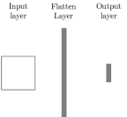
Let us now describe the NN architectures used in our numerical experiment, see also Figure 3.
Refer to caption
(a) Shallow NN with one dense layer.
Refer to caption
(b) Convolutional NN (LeNet-1) with two convolutional and two pooling layers, and one dense layer.
Figure 3: Architectures of the NNs used in the experiments of Section 4.

Each input image is a matrix of dimension 28×28282828\times 28 with entries valued between 00 and 111 depending on the grayscale of the respective pixel. For the shallow neural net (see Figure 3(a)) the image is first reshaped to a vector x728𝑥superscript728x\in\mathbb{R}^{728} before being passed through a dense layer of the form ReLU(Wx+b)ReLU𝑊𝑥𝑏\operatorname*{ReLU}(Wx+b) with weight matrix W10×728𝑊superscript10728W\in\mathbb{R}^{10\times 728} and bias b10𝑏superscript10b\in\mathbb{R}^{10}. The CNN architecture (see Figure 3(b)) is similar to the one of the LeNet-1, cf. [13, Section III.C.7]. Its first convolution layer has four kernels of size 5×5555\times 5 with zero padding and ReLUReLU\operatorname*{ReLU} activation and is followed by the first max pooling layer with 2×2222\times 2 kernel size and stride 222. The second convolution layer, again with ReLUReLU\operatorname*{ReLU} activation, has three convolution kernels of size 5×5555\times 5 with zero padding, where each kernel is applied to each of the four channels from the previous layer. It is followed by a max pooling layer of the same type as before. The resulting tensor of size 12×4×4124412\times 4\times 4 is then flattened and passed through a dense layer with ReLUReLU\operatorname*{ReLU} activation. For both networks we include a batch normalization step after the activation, which entails a considerably faster training process. Moreover, in the final layers a softmax activation function s𝑠s with (s())k=exp(()k)/=09exp(())subscript𝑠𝑘subscript𝑘superscriptsubscript09subscript(s(\cdot))_{k}=\exp((\cdot)_{k})/\sum_{\ell=0}^{9}\exp((\cdot)_{\ell}) is applied so that the 101010-dimensional output vector can be interpreted as the probability of the associated digit. In total, the number of unknowns to be trained in case of the shallow NN is 785078507850, which compares to 211221122112 free parameters for the CNN. We denote the parameters of the NN by θ𝜃\theta and its forward pass by fθsubscript𝑓𝜃f_{\theta}.

As a loss function during training we use the categorical crossentropy loss (y^,y)=k=09yklog(y^k)^𝑦𝑦superscriptsubscript𝑘09subscript𝑦𝑘subscript^𝑦𝑘\ell(\widehat{y},y)=-\sum_{k=0}^{9}y_{k}\log\left(\widehat{y}_{k}\right) with y^=fθ(x)^𝑦subscript𝑓𝜃𝑥\widehat{y}=f_{\theta}(x) denoting the output of the NN for a training sample (x,y)𝑥𝑦(x,y) consisting of image and label. This gives rise to the objective function (θ)=1Mm=1M(fθ(xm),ym)𝜃1𝑀superscriptsubscript𝑚1𝑀subscript𝑓𝜃superscript𝑥𝑚superscript𝑦𝑚{\cal E}(\theta)=\frac{1}{M}\sum_{m=1}^{M}\ell(f_{\theta}(x^{m}),y^{m}) when (xm,ym)m=1Msuperscriptsubscriptsuperscript𝑥𝑚superscript𝑦𝑚𝑚1𝑀(x^{m},y^{m})_{m=1}^{M} denote the training samples. When evaluating the performance of the NN we evaluate the accuracy on a test set by counting the number of successful predictions.

The used implementation of anisotropic CBO combines ideas presented in [9, Section 2.2] with the algorithm proposed in [4]. More precisely, it employs random mini-batch ideas when evaluating the objective function {\cal E} and when computing the consensus point vαsubscript𝑣𝛼v_{\alpha}, meaning that {\cal E} is only evaluated on a random subset of size nsubscript𝑛n_{\cal E} of the training dataset and vαsubscript𝑣𝛼v_{\alpha} is only computed from a random subset of size nNsubscript𝑛𝑁n_{N} of all agents. While this reduces the computational complexity, it simultaneously increases the stochasticity, which enhances the ability to escape from local optima. Furthermore, inspired by Simulated Annealing, a cooling strategy for the parameters α𝛼\alpha and σ𝜎\sigma is used as well as a variance-based particle reduction technique similar to ideas from genetic algorithms. More specifically, α𝛼\alpha is multiplied by 222 after each epoch, while the diffusion parameter σ𝜎\sigma follows the schedule σepoch=σ0/log2(epoch+2)subscript𝜎𝑒𝑝𝑜𝑐subscript𝜎0subscript2𝑒𝑝𝑜𝑐2\sigma_{epoch}=\sigma_{0}/\log_{2}(epoch+2). For our experiments we choose the parameters λ=1𝜆1\lambda=1, σ0=0.4subscript𝜎00.4\sigma_{0}=\sqrt{0.4} and αinitial=50subscript𝛼𝑖𝑛𝑖𝑡𝑖𝑎𝑙50\alpha_{initial}=50, and discrete time step size Δt=0.1Δ𝑡0.1\Delta t=0.1 for training both the shallow and convolutional NN. We use N=1000𝑁1000N=1000 agents, which are initialized according to 𝒩((0,,0)T,Id)𝒩superscript00𝑇Id{\cal N}\big{(}(0,\dots,0)^{T},\mathrm{Id}\big{)}. The mini-batch sizes are n=60subscript𝑛60n_{\cal E}=60 and nN=100subscript𝑛𝑁100n_{N}=100 and despite vαsubscript𝑣𝛼v_{\alpha} being computed only on a basis of nNsubscript𝑛𝑁n_{N} particles, all N𝑁N particles are updated in every time step, referred to as the full update in [4]. We emphasize that hyperparameters have not been tuned extensively.

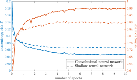
In Figure 4 we report the results of our experiment.
Refer to caption
Figure 4: Comparison of the performances of a shallow (dashed lines) and convolutional (solid lines) NN with architectures as described in Figures 3(a) and 3(b), when trained with a discretized version of the anisotropic CBO dynamics (1). Depicted are the accuracies on a test dataset (orange lines) and the values of the objective function {\cal E} (blue lines), which was chosen to be the categorical crossentropy loss on a random sample of the training set.

While achieving a test accuracy of about 89%percent8989\% for the shallow NN after as few as 444 epochs, we obtain almost 97%percent9797\% accuracy with the CNN. For comparison, when trained with backpropagation with finely tuned parameters, a comparable CNN achieves 98.3%percent98.398.3\% accuracy, cf. [13, Figure 9]. In view of these results, CBO can be regarded as a successful optimizer for machine learning tasks, which performs comparably to the state of the art. At the same time it is worth highlighting that CBO is extremely versatile and customizable, does not require gradient information or substantial hyperparameter tuning and has the potential to be parallelized.

5 Conclusion

In this paper we establish the global convergence of anisotropic consensus-based optimization (CBO) to the global minimizer in mean-field law with dimension-independent convergence rate by adapting the proof technique developed in [8]. It is based on the insight that the dynamics of individual agents follow, on average, the gradient flow dynamics of the map vvv22maps-to𝑣subscriptsuperscriptnorm𝑣superscript𝑣22v\mapsto\left\|{v-v^{*}}\right\|^{2}_{2}. Furthermore, by utilizing the implementation of anisotropic CBO suggested in [4], we demonstrate the practicability of the method by training the well-known LeNet-1 on the MNIST data set, achieving 97% accuracy after few epochs with just 1000 particles. In subsequent work we plan to extend our theoretical understanding to the finite particle regime, and aim to provide extensive numerical studies in the future.

5.0.1 Acknowledgements.

MF acknowledges the support of the DFG Project “Identification of Energies from Observations of Evolutions” and the DFG SPP 1962 “Non-smooth and Complementarity-Based Distributed Parameter Systems: Simulation and Hierarchical Optimization”. KR acknowledges the financial support from the Technical University of Munich – Institute for Ethics in Artificial Intelligence (IEAI).

References

  • [1] Aarts, E., Korst, J.: Simulated annealing and Boltzmann machines. A stochastic approach to combinatorial optimization and neural computing. Wiley-Interscience Series in Discrete Mathematics and Optimization, John Wiley & Sons, Ltd., Chichester (1989)
  • [2] Carrillo, J.A., Choi, Y.P., Totzeck, C., Tse, O.: An analytical framework for consensus-based global optimization method. Math. Models Methods Appl. Sci. 28(6), 1037–1066 (2018)
  • [3] Carrillo, J.A., Fornasier, M., Toscani, G., Vecil, F.: Particle, kinetic, and hydrodynamic models of swarming. In: Mathematical modeling of collective behavior in socio-economic and life sciences, pp. 297–336. Model. Simul. Sci. Eng. Technol., Birkhäuser Boston, Boston, MA (2010)
  • [4] Carrillo, J.A., Jin, S., Li, L., Zhu, Y.: A consensus-based global optimization method for high dimensional machine learning problems. ESAIM Control Optim. Calc. Var. 27(suppl.), Paper No. S5, 22 (2021)
  • [5] Dorigo, M., Blum, C.: Ant colony optimization theory: a survey. Theoret. Comput. Sci. 344(2-3), 243–278 (2005)
  • [6] Fogel, D.B.: Evolutionary computation. Toward a new philosophy of machine intelligence. IEEE Press, Piscataway, NJ, second edn. (2000)
  • [7] Fornasier, M., Huang, H., Pareschi, L., Sünnen, P.: Anisotropic diffusion in consensus-based optimization on the sphere. arXiv preprint arXiv:2104.00420 (2021)
  • [8] Fornasier, M., Klock, T., Riedl, K.: Consensus-based optimization methods converge globally in mean-field law. arXiv preprint arXiv:2103.15130 (2021)
  • [9] Fornasier, M., Pareschi, L., Huang, H., Sünnen, P.: Consensus-based optimization on the sphere: Convergence to global minimizers and machine learning. Journal of Machine Learning Research 22(237), 1–55 (2021)
  • [10] Holland, J.H.: Adaptation in natural and artificial systems. An introductory analysis with applications to biology, control, and artificial intelligence. University of Michigan Press, Ann Arbor, Mich. (1975)
  • [11] Huang, H., Qiu, J.: On the mean-field limit for the consensus-based optimization. arXiv preprint arXiv:2105.12919 (2021)
  • [12] Kennedy, J., Eberhart, R.: Particle swarm optimization. In: Proceedings of ICNN’95 - International Conference on Neural Networks. vol. 4, pp. 1942–1948. IEEE (1995)
  • [13] LeCun, Y., Bottou, L., Bengio, Y., Haffner, P.: Gradient-based learning applied to document recognition. Proceedings of the IEEE 86(11), 2278–2324 (1998)
  • [14] LeCun, Y., Cortes, C., Burges, C.: MNIST handwritten digit database. http://yann.lecun.com/exdb/mnist/ (2010)
  • [15] Miller, P.D.: Applied asymptotic analysis, Graduate Studies in Mathematics, vol. 75. American Mathematical Society, Providence, RI (2006)
  • [16] Pinnau, R., Totzeck, C., Tse, O., Martin, S.: A consensus-based model for global optimization and its mean-field limit. Math. Models Methods Appl. Sci. 27(1), 183–204 (2017)
  • [17] Rastrigin, L.: The convergence of the random search method in the extremal control of a many parameter system. Automaton & Remote Control 24, 1337–1342 (1963)
  • [18] Toscani, G.: Kinetic models of opinion formation. Commun. Math. Sci. 4(3), 481–496 (2006)