An Unsupervised Deep Unfolding Framework for Robust Symbol Level Precoding

Abdullahi Mohammad,  Christos Masouros,  and Yiannis Andreopoulos
Abstract

Symbol Level Precoding (SLP) has attracted significant research interest due to its ability to exploit interference for energy-efficient transmission. This paper proposes an unsupervised deep-neural network (DNN) based SLP framework. Instead of naively training a DNN architecture for SLP without considering the specifics of the optimization objective of the SLP domain, our proposal unfolds a power minimization SLP formulation based on the interior point method (IPM) proximal ‘log’ barrier function. Furthermore, we extend our proposal to a robust precoding design under channel state information (CSI) uncertainty. The results show that our proposed learning framework provides near-optimal performance while reducing the computational cost from \mathbcalO(n7.5)\mathbcal𝑂superscript𝑛7.5\mathbcal{O}(n^{7.5}) to \mathbcalO(n3)\mathbcal𝑂superscript𝑛3\mathbcal{O}(n^{3}) for the symmetrical system case where n=number of transmit antennas=number of users𝑛number of transmit antennasnumber of usersn=\text{number of transmit antennas}=\text{number of users}. This significant complexity reduction is also reflected in a proportional decrease in the proposed approach’s execution time compared to the SLP optimization-based solution.

Index Terms:
Symbol level precoding, Constructive Interference, downlink beamforming, power minimization, Deep Neural Networks.

I Introduction

Interference has been known to yield a decrease in the throughput and communication reliability of a downlink multi-user multiple-input single-output (MU-MISO) wireless system. Traditionally, interference is regarded as the limiting factor against the ever-increasing needs for transmission rates and quality of service (QoS) in fifth-generation (5G) wireless communication systems and beyond [1, 2, 3]. However, recent studies on interference exploitation have transformed the traditional paradigm in which known inferences are effectively managed [1, 2, 4, 3, 5]. Consequently, transmit beamforming techniques for the downlink channels for power minimization problems under specific QoS become imperative for high-throughput systems under interference.

The idea of exploiting interference was first introduced by Masouros and Alsusa [6], where instantaneous interference was classified into constructive and destructive. Initial suboptimal approaches to exploit constructive interference (CI) were first introduced by Masouros et al. [7][8]. The first form of optimization-based CI precoding was introduced in the context of vector perturbation precoding through a quadratic optimization approach [9]. A convex optimization-based CI scheme termed symbol-level-precoding technique was proposed first with strict phase constraints on the received constellation point [10], and with a robust relaxed-angle formulation [2]. We refer to recent work [9, 10, 11, 12, 13] for more details on the optimization-based CI precoding techniques.

As a result of the performance gains over conventional block-level-precoding (BLP) schemes, the idea of CI has been applied in many domains, such as vector perturbation [14], wireless information and power transfer [15], mutual coupling exploitation [16], multiuser MISO downlink channel [17], directional modulation [18], relay and cognitive radio [1, 19]. Despite the superior performance offered by CI-based precoding methods, their increased computational complexity can hinder their practical application when performed on a symbol-by-symbol basis. To address this, Li and Masouros [20] proposed an iterative closed-form precoding design with optimal performance for CI exploitation in the MISO downlink by driving the optimal precoder’s mathematical Lagrangian expression and Karush–Kuhn–Tucker conditions for optimization with both strict and relaxed phase rotations.

Lately, there is growing interest in using deep neural networks (DNNs) for wireless physical layer design [21, 22, 23]. More relevant to this work are the learning-based precoding schemes for MU-MISO downlink transmission [24, 25, 26, 27, 28]. The benefit of using DNNs is that the computational burden of the learning algorithm can be controlled via online training, and a variety of loss functions can be used for each optimization objective. One of the earliest attempts of using DNNs models for beamforming design was the work of Alkhateeb et al. [22], where a learning-based coordinated beamforming technique was proposed for link reliability and frequent poor hand-off between base stations (BSs) in millimeter-wave (mmWave) communications. Kerret and Gesbert [29] introduced DNNs precoding scheme to address the “Team Decision problems” for a decentralized decision making in multiple-input-multiple-output (MIMO) settings. Huang et al. [24] proposed a fast beamforming design based on unsupervised learning that yielded performance close to that of the weighted minimum mean-squared error (WMMSE) algorithm. A DNN-based precoding strategy that utilized a heuristic solution structure of the downlink beamforming was proposed by Huang et al. [27]. Furthermore, Xia et al. [26] developed deep convolutional neural networks (CNNs) framework for downlink beamforming optimization. The framework exploits expert knowledge based on the known structure of optimal iterative solutions for sum-rate maximization, power minimization, and SINR balancing problems.

DNN methods are typically used for unconstrained optimization problems. Therefore, most of the DNN-based strategies for wireless physical layer designs are based on supervised learning to approximate the optimal solutions. Using such approaches, the constraints are implicitly contained in the training dataset obtained from conventional optimization solutions. However, if obtaining optimal solutions via traditional optimization methods is very computationally expensive (or infeasible), using supervised learning methods for DNN-based method may not be practical.

Furthermore, the common approach for solving constrained optimization with DNN for wireless physical layer design is via function approximation. It involves solving the problem, first using iterative algorithms or convex optimization techniques, and finally approximating the optimal solution with a DNN architecture [25, 27, 26]. Accordingly, the major drawback of these proposals is that the efficacy of supervised learning is bounded by the assumptions and accuracy of the optimal solutions obtained from the structural optimization algorithm.

This work proposes an unsupervised learning-based approach for precoding design by exploiting known interference in MU-MISO systems for the power minimization problem under SINR constraints. The learning framework is designed by unfolding an interior point method (IPM) iterative algorithm via ‘log’ barrier function. The proposed learning-based precoding scheme does not require generating the training dataset from the conventional optimization solutions, thereby saving considerable computational effort and time. Our contributions are summarized below:

  • We introduce an unsupervised DNN-based power minimization SLP scheme for MU-MISO downlink transmission. The proposed framework is designed by unfolding an IPM algorithm via a ‘log’ barrier function that exploits the convexity associated with the SLP inequality constraints. The learning framework utilizes the domain knowledge to derive the Lagrange function of the original SLP optimization as a loss function. This is used to train the network in an unsupervised mode to learn a set of Lagrangian multipliers that directly minimize the objective function to satisfy the constraints. A regularization parameter is added to the Lagrange function to aid the training convergence, and we provide detailed formulations leading to the unfolded unsupervised learning architecture for constrained optimization problems.

  • We extend the formulation to design a robust learning-based precoder where the uncertainty in channel estimation is considered.

  • We derive analytic expressions for the computational complexity of various SLP and the proposed unsupervised learning precoding schemes. Our analysis demonstrates that the proposed deep unfolding (DU) framework offers a theoretical, computational complexity reduction from \mathbcalO(n7.5)\mathbcal𝑂superscript𝑛7.5\mathbcal{O}(n^{7.5}) to \mathbcalO(n3)\mathbcal𝑂superscript𝑛3\mathbcal{O}(n^{3}) for the symmetrical system case where n𝑛n = number of transmit antennas = number of users This is reflected in a commensurate decrease in the execution time as compared to the SLP optimization-based method.

The remainder of the paper is organized as follows: The system model and the methods for traditional precoding and SLP optimization-based for downlink MU-MISO system are presented in Section II. The proposed unsupervised DU-based precoding designs under perfect channel condition for power minimization are introduced in Section III and extension to a robust precoding design under uncertainty channel condition is described in Section IV. Section V presents detailed analytic computational complexity evaluation of the proposed precoding schemes. Simulations and results are presented in Section VI. Finally, Section VII summarizes and concludes the paper.

Notations: We use bold uppercase symbols for matrices, bold lowercase symbols for vectors and lowercase symbols for scalars. The \mathbcall2\mathbcalsubscript𝑙2\mathbcal{l}_{2}-norm and \mathbcall1\mathbcalsubscript𝑙1\mathbcal{l}_{1}-norm are denoted by 2subscriptdelimited-∥∥2\left\lVert\cdot\right\rVert_{2} and 1subscriptdelimited-∥∥1\left\lVert\cdot\right\rVert_{1}, respectively. The |||\cdot| represents the absolute value and 𝜽isubscript𝜽𝑖\bm{\theta}_{i} is the i-th trainable parameter associated with DNN layers. Operators Re()(\cdot) and Im()(\cdot) represent real and imaginary parts of a complex vector, respectively. Finally, notations \mathbcalL()\mathbcal𝐿\mathbcal{L}(\cdot) and \mathbcalH()\mathbcal𝐻\mathbcal{H}(\cdot) are reserved for the loss and parameter update functions, respectively.

II System Model and Problem Description

II-A Conventional Block Level Precoding for Power Minimization

Consider a signle-cell downlink channel with Ntsubscript𝑁𝑡N_{t} transmit antennas at the BS transmitting to K𝐾K single-antenna users. Assume a quasi-static flat-fading channel between the BS and the users, denoted by 𝐡iNt×1subscript𝐡𝑖superscriptsubscript𝑁𝑡1\mathbf{h}_{i}\in\mathbb{C}^{{N}_{t}\times 1}. The received signal at user i𝑖i is given by

yi=𝐡iTk=1K𝐰ksk+vi=𝐡iTk=1K𝐰kej(φkφi)si+visubscript𝑦𝑖subscriptsuperscript𝐡𝑇𝑖subscriptsuperscript𝐾𝑘1subscript𝐰𝑘subscript𝑠𝑘subscript𝑣𝑖subscriptsuperscript𝐡𝑇𝑖superscriptsubscript𝑘1𝐾subscript𝐰𝑘superscript𝑒𝑗subscript𝜑𝑘subscript𝜑𝑖subscript𝑠𝑖subscript𝑣𝑖\begin{split}y_{i}&=\mathbf{h}^{T}_{i}\sum\limits^{K}_{k=1}\mathbf{w}_{k}{s}_{k}+v_{i}\\ &=\mathbf{h}^{T}_{i}\sum_{k=1}^{K}\mathbf{w}_{k}e^{j(\varphi_{k}-\varphi_{i})}{s}_{i}+v_{i}\end{split} (1)

where 𝐡isubscript𝐡𝑖\mathbf{h}_{i}, 𝐰isubscript𝐰𝑖\mathbf{w}_{i}, sisubscript𝑠𝑖{s}_{i}, visubscript𝑣𝑖{v}_{i} and φisubscript𝜑𝑖\varphi_{i} represent the channel vector, precoding vector, data symbol, received noise and phase rotation for the i-th user. Conventionally, the power minimization problem seeks to minimize the average transmit power by treating all interference as detrimental subject to QoS constraints as defined below [30]

min{𝐰𝐢}subscript𝐰𝐢min\displaystyle\underset{\mathbf{\{w_{i}\}}}{\text{min}} i=1K𝐰k22superscriptsubscript𝑖1𝐾superscriptsubscriptdelimited-∥∥subscript𝐰𝑘22\displaystyle{\sum_{i=1}^{K}\left\lVert\mathbf{w}_{k}\right\rVert_{2}^{2}} (2)
s.t. |𝐡iT𝐰i|2k=1,ki|𝐡iT𝐰k|2+v0Γi,i.superscriptsuperscriptsubscript𝐡𝑖𝑇subscript𝐰𝑖2subscriptformulae-sequence𝑘1𝑘𝑖superscriptsuperscriptsubscript𝐡𝑖𝑇subscript𝐰𝑘2subscript𝑣0subscriptΓ𝑖for-all𝑖\displaystyle\frac{|\mathbf{h}_{i}^{T}\mathbf{w}_{i}|^{2}}{\sum_{k=1,k\neq i}|\mathbf{h}_{i}^{T}\mathbf{w}_{k}|^{2}+{v}_{0}}\geq\Gamma_{i}\ ,\ \forall{i}.

where ΓisubscriptΓ𝑖\Gamma_{i} is the SINR threshold of the i-th user. It has been proven that problem (2) is suboptimal from an instantaneous point of view, as it does not take into account the fact that interference can constructively enhance the received signal power [8].
Refer to caption
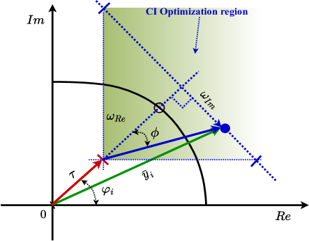
Figure 1: Generic geometrical optimization regions for interference exploitation for Precoding design in 𝕄𝕄\mathbb{M}-PSK [2].

II-B Power Minimization via Symbol-Level Precoding

With the aim of utilizing the instantaneous interference in a multi-user downlink channel scenario, the interference can be categorized into constructive and destructive based on the known standards described [31]. Based on this, CI is defined as the interference that nudges the received symbols off the modulated-symbol constellation’s decision thresholds [2]. Fig. 1 shows the generic geometrical representation of the CI, where the received signal is expressed as 𝐲¯i𝐡iTk=1K𝐰kej(φkφ1)subscript¯𝐲𝑖superscriptsubscript𝐡𝑖𝑇superscriptsubscript𝑘1𝐾subscript𝐰𝑘superscript𝑒𝑗subscript𝜑𝑘subscript𝜑1\bar{\mathbf{y}}_{i}\triangleq\mathbf{h}_{i}^{T}\sum_{k=1}^{K}\mathbf{w}_{k}{e}^{j(\varphi_{k}-\varphi_{1})}. From the received symbol expression, the real and imaginary parts are respectively given by: 𝝎Re=Re(𝐲¯i)subscript𝝎𝑅𝑒Resubscript¯𝐲𝑖\bm{\omega}_{Re}=\text{Re}({\bar{\mathbf{y}}_{i}}) and 𝝎Im=Im(𝐲¯i)subscript𝝎𝐼𝑚Imsubscript¯𝐲𝑖\bm{\omega}_{Im}=\text{Im}({\bar{\mathbf{y}}_{i}}). In Fig. 1, we show an indicative example corresponding to the constellation point 1+j1𝑗1+j in the QPSK constellation, where the green shaded area represents the constructive region of the constellation, based on the minimum distance (τ)𝜏(\tau) from the decision boundaries. The value of τ𝜏\tau is determined by the SNR constraints. In line with the preceding description, problem (2) is adjusted to include CI in the power minimization formulation. This allows the interfering signals to align with the symbol of interest constructively through precoding, contributing to the desired signal. Therefore, for 𝕄𝕄\mathbb{M}-PSK, the power minimization SLP can be reformulated based on the constructive/destructive interference classification criteria [32]. The maximum phase shift in the CI region is given by ϕ=±π𝕄italic-ϕplus-or-minus𝜋𝕄\phi=\pm\frac{\pi}{\mathbb{M}}, where 𝕄𝕄\mathbb{M} is the modulation order. Therefore, the SLP optimization is given by [2]

min{𝐰𝐢}k=1K𝐰kej(φkφ1)22s.t.|Im(𝐡iTk=1K𝐰kej(φkφi))|(Re(𝐡iTk=1K𝐰kej(φkφi))Γiv0)tanϕ,i.missing-subexpressionsubscript𝐰𝐢minmissing-subexpressionsuperscriptsubscriptdelimited-∥∥superscriptsubscript𝑘1𝐾subscript𝐰𝑘superscript𝑒𝑗subscript𝜑𝑘subscript𝜑122missing-subexpressions.t.missing-subexpressionImsuperscriptsubscript𝐡𝑖𝑇superscriptsubscript𝑘1𝐾subscript𝐰𝑘superscript𝑒𝑗subscript𝜑𝑘subscript𝜑𝑖absentmissing-subexpressionmissing-subexpressionmissing-subexpressionResuperscriptsubscript𝐡𝑖𝑇superscriptsubscript𝑘1𝐾subscript𝐰𝑘superscript𝑒𝑗subscript𝜑𝑘subscript𝜑𝑖subscriptΓ𝑖subscript𝑣0tanitalic-ϕfor-all𝑖\begin{aligned} &\underset{\mathbf{\{w_{i}\}}}{\text{min}}&&{\left\lVert\sum_{k=1}^{K}\mathbf{w}_{k}{e}^{j(\varphi_{k}-\varphi_{1})}\right\rVert_{2}^{2}}\\ &\text{s.t.}&&\left|\text{Im}{\left(\mathbf{h}_{i}^{T}\sum_{k=1}^{K}\mathbf{w}_{k}e^{j(\varphi_{k}-\varphi_{i})}\right)}\right|\leq\\ &&&\left(\text{Re}{\left(\mathbf{h}_{i}^{T}\sum_{k=1}^{K}\mathbf{w}_{k}e^{j(\varphi_{k}-\varphi_{i})}\right)-\sqrt{\Gamma_{i}v_{0}}}\right)\text{tan}\phi\ ,\ \forall{i}.\end{aligned}

(3)

III Learning-Based Power minimization for SLP

This section presents the formulation of a learning-based CI power minimization problem for SLP. Throughout this section, we assume a perfect CSI known at the BS.

Motivated by the recent adoption of an IPM for image restoration [33], we propose an unsupervised learning framework that unfolds a constrained optimization problem into a sequence of learning layers/iterations for a multi-user MISO beamforming. We first convert (3) into a standard IPM formulation containing a slack variable, where necessary. The measure of the fidelity of the solution to (3) is determined by learning a set of penalty parameters in the form of Lagrange multipliers associated with the constraints. From (3), we define the following

𝐡^i=𝐡ik=1Kej(φkφi)subscript^𝐡𝑖subscript𝐡𝑖superscriptsubscript𝑘1𝐾superscript𝑒𝑗subscript𝜑𝑘subscript𝜑𝑖\hat{\mathbf{h}}_{i}=\mathbf{h}_{i}\sum_{k=1}^{K}e^{j(\varphi_{k}-\varphi_{i})} (4)
𝐰=k=1K𝐰k.𝐰superscriptsubscript𝑘1𝐾subscript𝐰𝑘{\mathbf{w}}=\sum_{k=1}^{K}\mathbf{w}_{k}. (5)

Accordingly, to ease the analysis, we partition the complex rotations into the real and imaginary parts as follows

𝐡^isubscript^𝐡𝑖\displaystyle\hat{\mathbf{h}}_{i} =𝐡^Ri+j𝐡^Iiabsentsubscript^𝐡𝑅𝑖𝑗subscript^𝐡𝐼𝑖\displaystyle=\hat{\mathbf{h}}_{Ri}+j\hat{\mathbf{h}}_{Ii} (6a)
𝐰𝐰\displaystyle\mathbf{w} =𝐰R+j𝐰Iabsentsubscript𝐰𝑅𝑗subscript𝐰𝐼\displaystyle=\mathbf{w}_{R}+j\mathbf{w}_{I} (6b)

where 𝐡^Ri=Re(𝐡^i)subscript^𝐡𝑅𝑖Resubscript^𝐡𝑖\hat{\mathbf{h}}_{Ri}=\text{Re}(\hat{\mathbf{h}}_{i}), 𝐡^Ii=Im(𝐡^i)subscript^𝐡𝐼𝑖Imsubscript^𝐡𝑖\hat{\mathbf{h}}_{Ii}=\text{Im}(\hat{\mathbf{h}}_{i}), 𝐰R=Re(𝐰)subscript𝐰𝑅Re𝐰\mathbf{w}_{R}=\text{Re}(\mathbf{w}) and 𝐰I=Im(𝐰)subscript𝐰𝐼Im𝐰\mathbf{w}_{I}=\text{Im}(\mathbf{w}).

The product of complex rotations of (6a) and (6b) can be written as

𝐡^i𝐰=(𝐡^Ri+j𝐡^Ii)(𝐰R+j𝐰I).subscript^𝐡𝑖𝐰subscript^𝐡𝑅𝑖𝑗subscript^𝐡𝐼𝑖subscript𝐰𝑅𝑗subscript𝐰𝐼\hat{\mathbf{h}}_{i}\mathbf{w}=(\hat{\mathbf{h}}_{Ri}+j\hat{\mathbf{h}}_{Ii})(\mathbf{w}_{R}+j\mathbf{w}_{I}). (7)

Using (6), the real and imaginary parts of (7) can be written in vector forms as follows

Re(𝐡^i𝐰)Resubscript^𝐡𝑖𝐰\displaystyle\text{Re}(\hat{\mathbf{h}}_{i}\mathbf{w}) =[𝐡^Ri𝐡^Ii][𝐰R𝐰I]absentmatrixsubscript^𝐡𝑅𝑖subscript^𝐡𝐼𝑖matrixsubscript𝐰𝑅subscript𝐰𝐼\displaystyle=\begin{bmatrix}\hat{\mathbf{h}}_{Ri}\ \ \hat{\mathbf{h}}_{Ii}\ \end{bmatrix}\begin{bmatrix}\mathbf{w}_{R}\\ -\mathbf{w}_{I}\ \end{bmatrix} (8a)
Im(𝐡^i𝐰)Imsubscript^𝐡𝑖𝐰\displaystyle\text{Im}(\hat{\mathbf{h}}_{i}\mathbf{w}) =[𝐡^Ri𝐡^Ii][𝐰I𝐰R]absentmatrixsubscript^𝐡𝑅𝑖subscript^𝐡𝐼𝑖matrixsubscript𝐰𝐼subscript𝐰𝑅\displaystyle=\begin{bmatrix}\hat{\mathbf{h}}_{Ri}\ \ \hat{\mathbf{h}}_{Ii}\ \end{bmatrix}\begin{bmatrix}\mathbf{w}_{I}\\ \mathbf{w}_{R}\ \end{bmatrix} (8b)

Let 𝚲=[𝐡^Ri𝐡^Ii]T𝚲superscriptsubscript^𝐡𝑅𝑖subscript^𝐡𝐼𝑖𝑇\bm{\Lambda}=[\hat{\mathbf{h}}_{Ri}\ \ \hat{\mathbf{h}}_{Ii}]^{T}, 𝐰1=[𝐰R𝐰I]Tsubscript𝐰1superscriptdelimited-[]subscript𝐰𝑅subscript𝐰𝐼𝑇\mathbf{w}_{1}=[\mathbf{w}_{R}\ -\mathbf{w}_{I}]^{T} and 𝐰2=[𝐰I𝐰R]Tsubscript𝐰2superscriptsubscript𝐰𝐼subscript𝐰𝑅𝑇\mathbf{w}_{2}=[\mathbf{w}_{I}\ \ \mathbf{w}_{R}]^{T}

Re(𝐡^iT𝐰)=𝚲iT𝐰1andIm(𝐡^iT𝐰)=𝚲iT𝚷𝐰1Resuperscriptsubscript^𝐡𝑖𝑇𝐰superscriptsubscript𝚲𝑖𝑇subscript𝐰1andImsuperscriptsubscript^𝐡𝑖𝑇𝐰superscriptsubscript𝚲𝑖𝑇𝚷subscript𝐰1\text{Re}(\hat{\mathbf{h}}_{i}^{T}\mathbf{w})=\bm{\Lambda}_{i}^{T}\mathbf{w}_{1}\ \text{and}\ \text{Im}(\hat{\mathbf{h}}_{i}^{T}\mathbf{w})=\bm{\Lambda}_{i}^{T}\bm{\Pi}\mathbf{w}_{1} (9)

where

𝐰2=𝚷𝐰1and𝚷=[𝐎Nt𝐈Nt𝐈Nt𝐎Nt];2Nt×2Nt,{\mathbf{w}_{2}=\bm{\Pi}}\mathbf{w}_{1}\ \text{and}\ \bm{\Pi}=\begin{bmatrix}\mathbf{O}_{N_{t}}&-\mathbf{I}_{N_{t}}\\ \mathbf{I}_{N_{t}}&\mathbf{O}_{N_{t}}\end{bmatrix};\ \in\mathbb{R}^{2N_{t}\times 2N_{t}}, (10)

Note that 𝐈Ntsubscript𝐈subscript𝑁𝑡\mathbf{I}_{N_{t}} is the identity matrix and 𝐎Ntsubscript𝐎subscript𝑁𝑡\mathbf{O}_{N_{t}} the matrix of zeros, respectively. Using the above definitions, problem (3) can be recast into its mutlicast formulation [2]

min{𝐰𝟏}subscript𝐰1min\displaystyle\underset{\mathbf{\{w_{1}\}}}{\text{min}} 𝐰122superscriptsubscriptdelimited-∥∥subscript𝐰122\displaystyle{\left\lVert\mathbf{w}_{1}\right\rVert_{2}^{2}} (11)
s.t. |𝚲iT𝚷𝐰1|(𝚲iT𝐰1Γiv0)tanϕ,isuperscriptsubscript𝚲𝑖𝑇𝚷subscript𝐰1superscriptsubscript𝚲𝑖𝑇subscript𝐰1subscriptΓ𝑖subscript𝑣0tanitalic-ϕfor-all𝑖\displaystyle\left|{\bm{\Lambda}_{i}^{T}\bm{\Pi}\mathbf{w}_{1}}\right|\leq\left(\bm{\Lambda}_{i}^{T}\mathbf{w}_{1}-\sqrt{\Gamma_{i}v_{0}}\right)\text{tan}\phi\ ,\ \forall{i}

III-A Interior Point Method

Consider a general form of a nonlinear constrained optimization of the form [34]

min𝐱𝐍𝐱superscript𝐍min\displaystyle\underset{\mathbf{x\in{\mathbb{R}^{N}}}}{\text{min}} f(𝐱)𝑓𝐱\displaystyle{f(\mathbf{x})} (12)
s.t. g(𝐱)0𝑔𝐱0\displaystyle g(\mathbf{x})\geq 0
C(𝐱)=0,𝐶𝐱0\displaystyle\left.\begin{aligned} C(\mathbf{x})=0\end{aligned}\right.,

The rationale of adopting IPM is to substitute the initial constrained optimization problem by a chain of unconstrained sub-problems of the form

min𝐱𝐍f(𝐱)+λC(𝐱)+μB(𝐱).𝐱superscript𝐍min𝑓𝐱𝜆𝐶𝐱𝜇𝐵𝐱\displaystyle\underset{\mathbf{x\in{\mathbb{R}^{N}}}}{\text{min}}f(\mathbf{x})+\lambda{{C(\mathbf{x})}}+\mu{{B(\mathbf{x})}}. (13)

where B()ln()𝐵{B}(\cdot)\triangleq-\sum\ln{(\cdot)} is the logarithmic barrier function associated with inequality constraint with unbounded derivative at the boundary of the feasible domain, C()𝐶{C}(\cdot) is a function associated with equality constraint, μ𝜇\mu and λ𝜆\lambda are the Lagrangian multipliers for inequality and equality constraints, respectively. For K𝐾K users, we define a vector 𝝁[μ1,,μK]𝝁subscript𝜇1subscript𝜇𝐾\bm{\mu}\triangleq[\mu_{1},\cdots,\mu_{K}].

Following the above line of argument, the unconstrained sequence of (11) per user can be written as

min𝐰𝟐𝐍𝐭×𝟏f(𝐰1)+μB(𝐰1),𝐰superscript2subscript𝐍𝐭1min𝑓subscript𝐰1𝜇𝐵subscript𝐰1\displaystyle\underset{\mathbf{w\in{\mathbb{R}^{2N_{t}\times 1}}}}{\text{min}}f(\mathbf{w}_{1})+{\mu}{{B(\mathbf{w}_{1})}}, (14)

To facilitate the solution of (11) , we introduce additional notations. For every inequality constraint, γ{0,+}𝛾0\gamma\in\{0,+\infty\} and 𝐰12Nt×1subscript𝐰1superscript2subscript𝑁𝑡1\mathbf{w}_{1}\in\mathbb{R}^{2N_{t}\times 1}, we define the proximity function as in [34] with respect to (14), which we shall later use to compute the projected gradient descent as

proxγμB(𝐰1)=subscriptprox𝛾𝜇𝐵subscript𝐰1absent\displaystyle\text{prox}_{\gamma{\mu}{B}}{(\mathbf{w}_{1})}= argmin𝐰𝟏𝟐𝐍𝐭×𝟏subscript𝐰1superscript2subscript𝐍𝐭1argmin\displaystyle\underset{\mathbf{w_{1}\in{\mathbb{R}^{2N_{t}\times{1}}}}}{\text{argmin}} 12𝐰0𝐰122+γμB(𝐰1),12superscriptsubscriptdelimited-∥∥subscript𝐰0subscript𝐰122𝛾𝜇𝐵subscript𝐰1\displaystyle{\frac{1}{2}\left\lVert\mathbf{w}_{0}-\mathbf{w}_{1}\right\rVert}_{2}^{2}+\gamma{\mu}{B}({\mathbf{w}_{1}}), (15)

where γ𝛾\gamma is the step-size for computing the gradients and 𝐰0subscript𝐰0\mathbf{w}_{0} is the initial value of the precoding vector. To convert (3) into its equivalent barrier function problem, we integrate the inequality constraint into the objective by translating it into a barrier term as follows [35]

min𝐰𝟏subscript𝐰1min\displaystyle\underset{\mathbf{w_{1}}}{\text{min}} f(𝐰1)μi=1pln(g(𝐰1i))𝑓subscript𝐰1𝜇superscriptsubscript𝑖1𝑝𝑔subscript𝐰1𝑖\displaystyle{f(\mathbf{w}_{1})}-{\mu}\sum_{i=1}^{p}{\ln{\left(g({\mathbf{w}}_{1i})\right)}} (16)
s.t. C(𝐰1)=0𝐶subscript𝐰10\displaystyle{{C(\mathbf{w}_{1})}=0}

where g(𝐰1)=(𝚲iT𝐰1Γiv0)tanϕ|𝚲iT𝚷𝐰1|𝑔subscript𝐰1superscriptsubscript𝚲𝑖𝑇subscript𝐰1subscriptΓ𝑖subscript𝑣0tanitalic-ϕsuperscriptsubscript𝚲𝑖𝑇𝚷subscript𝐰1g({\mathbf{w}}_{1})=\left(\bm{\Lambda}_{i}^{T}\mathbf{w}_{1}-\sqrt{\Gamma_{i}v_{0}}\right)\text{tan}\phi-\left|{\bm{\Lambda}_{i}^{T}\bm{\Pi}\mathbf{w}_{1}}\right| and p𝑝p is the number of the optimization variables.

Going back to our initial SPL optimization to apply this framework, first we rewrite the constraint of (11) as

a𝚲iT𝚷𝐰1b,𝑎superscriptsubscript𝚲𝑖𝑇𝚷subscript𝐰1𝑏{a}\leq{\bm{\Lambda}_{i}^{T}\bm{\Pi}\mathbf{w}_{1}}\leq{b}, (17)

where

a𝑎\displaystyle{a} =(𝚲iT𝚷𝐰1Γiv0)tanϕ,absentsuperscriptsubscript𝚲𝑖𝑇𝚷subscript𝐰1subscriptΓ𝑖subscript𝑣0tanitalic-ϕ\displaystyle=-\left(\bm{\Lambda}_{i}^{T}\bm{\Pi}\mathbf{w}_{1}-\sqrt{\Gamma_{i}v_{0}}\right){\text{tan}{\phi}}, (18a)
b𝑏\displaystyle{b} =(𝚲iT𝚷𝐰1Γiv0)tanϕ.absentsuperscriptsubscript𝚲𝑖𝑇𝚷subscript𝐰1subscriptΓ𝑖subscript𝑣0tanitalic-ϕ\displaystyle=\left(\bm{\Lambda}_{i}^{T}\bm{\Pi}\mathbf{w}_{1}-\sqrt{\Gamma_{i}v_{0}}\right){\text{tan}{\phi}}. (18b)

Therefore, the original problem (11) becomes

min{𝐰𝟏}subscript𝐰1min\displaystyle\underset{\mathbf{\{w_{1}\}}}{\text{min}} 𝐰122superscriptsubscriptdelimited-∥∥subscript𝐰122\displaystyle{\left\lVert\mathbf{w}_{1}\right\rVert_{2}^{2}} (19)
s.t. a𝚲iT𝚷𝐰1b,i.formulae-sequence𝑎superscriptsubscript𝚲𝑖𝑇𝚷subscript𝐰1𝑏for-all𝑖\displaystyle{a}\leq{\bm{\Lambda}_{i}^{T}\bm{\Pi}\mathbf{w}_{1}}\leq{b}\ ,\ \forall{i}.

It is apparent that the constraint of (19) is contained within a hyperslab [36].

III-A1 Hyperslab Constraints

Given the constraint in (19), the precoding vector 𝐰1subscript𝐰1\mathbf{w}_{1} is contained within a set of hyperslab 𝒞𝒞\mathcal{C} and also bounded by {a,b}𝑎𝑏\{{a},\ {b}\}. Therefore, 𝒞𝒞\mathcal{C} is defined as follows

\mathbcalC={𝐰1Nt×1}|a𝚲T𝚷𝐰1b.\mathbcal𝐶evaluated-atsubscript𝐰1superscriptsubscript𝑁𝑡1𝑎superscript𝚲𝑇𝚷subscript𝐰1𝑏\mathbcal{C}=\{\mathbf{w}_{1}\in\mathbb{R}^{N_{t}\times 1}\}|_{{a}\leq\bm{\Lambda}^{T}\bm{\Pi}\mathbf{w}_{1}\leq{b}}. (20)

For all γ>0𝛾0\gamma>0 and μ>0𝜇0{\mu}>0, a proximity barrier function related to (20) is given by

B(𝐰1)={ln(bw^1)ln(a+w^1),ifaw^1b+,otherwise\begin{array}[]{ll}{B}({\mathbf{w}}_{1})=\left\{\begin{aligned} &-\ln{\left({b}-\hat{{w}}_{1}\right)}-\ln{\left(-{a}+\hat{{w}}_{1}\right)},&&\text{if}\ -{a}\leq\hat{{w}}_{1}\leq{b}\\ &+\infty,&&\text{otherwise}\end{aligned}\right.\end{array}

(21)

where for convenience, we let w^1=𝚲iT𝚷𝐰1subscript^𝑤1superscriptsubscript𝚲𝑖𝑇𝚷subscript𝐰1\hat{{w}}_{1}=\bm{\Lambda}_{i}^{T}{\bm{\Pi}}{\mathbf{w}_{1}}.

III-B Proximity Operator for the SLP Formulation

To unfold (19) into learning framework using IPM, we use its equivalent proximity ‘log’ barrier function (21) and the proximal operator of γμB(𝐰1)𝛾𝜇𝐵subscript𝐰1\gamma{\mu}B(\mathbf{w}_{1}) for every 𝐰1subscript𝐰1\mathbf{w}_{1} defined as

Φ(𝐰1,γ,μ)=proxγ𝝁B(𝐰1)=𝐰1+X(𝐰1,γ,μ)𝚲iT𝐰1𝚲i22𝚲iΦsubscript𝐰1𝛾𝜇subscriptprox𝛾𝝁𝐵subscript𝐰1subscript𝐰1𝑋subscript𝐰1𝛾𝜇superscriptsubscript𝚲𝑖𝑇subscript𝐰1superscriptsubscriptnormsubscript𝚲𝑖22subscript𝚲𝑖\Phi(\mathbf{w}_{1},\gamma,{\mu})=\text{prox}_{\gamma\bm{\mu}{{B}}}{(\mathbf{w}_{1})}=\mathbf{w}_{1}+\frac{X(\mathbf{w}_{1},\gamma,{\mu})-\bm{\Lambda}_{i}^{T}\mathbf{w}_{1}}{\|\bm{\Lambda}_{i}\|_{2}^{2}}{\bm{\Lambda}_{i}} (22)

where X𝑋{X} is a typical solution of the following cubic equation of the form

x3(b+a+𝚲T𝐰1)x2+(ba+𝚲T𝐰1(b+a)2γμ𝚲22)x+(ba𝚲T𝐰1+γμ(b+a)𝚲22)=0.superscript𝑥3𝑏𝑎superscript𝚲𝑇subscript𝐰1superscript𝑥2𝑏𝑎superscript𝚲𝑇subscript𝐰1𝑏𝑎2𝛾𝜇superscriptsubscriptdelimited-∥∥𝚲22𝑥𝑏𝑎superscript𝚲𝑇subscript𝐰1𝛾𝜇𝑏𝑎superscriptsubscriptdelimited-∥∥𝚲220{x}^{3}-\left({b}+{a}+\bm{\Lambda}^{T}\mathbf{w}_{1}\right){x}^{2}+\\ \left({b}{a}+\bm{\Lambda}^{T}\mathbf{w}_{1}({b}+{a})-2\gamma{{\mu}}\|\bm{\Lambda}\|_{2}^{2}\right){x}\\ +\left(-{b}{a}\bm{\Lambda}^{T}\mathbf{w}_{1}+\gamma{\mu}\left({b}+{a}\right)\|\bm{\Lambda}\|_{2}^{2}\right)=0. (23)

It is important to note that the solution to (23) is obtained using the analytic solution of the cubic equation. To build the structure of the learning framework, as detailed in [33], we need to obtain the Jacobian matrix of Φ(𝐰1,γ,μ)Φsubscript𝐰1𝛾𝜇\Phi(\mathbf{w}_{1},\gamma,{\mu}) with respect to 𝐰1subscript𝐰1\mathbf{w}_{1} and the derivatives with respect to γ𝛾\gamma and μ𝜇\mu as follows

𝒥Φ(𝐰1)=𝐈2Nt+1𝚲i22×((bX(𝐰1,γ,μ))(aX(𝐰1,γ,μ))Υ(𝐰1,γ,μ)1)𝚲𝒊𝚲𝒊𝑻evaluated-atsubscript𝒥Φsubscript𝐰1subscript𝐈2subscript𝑁𝑡1superscriptsubscriptdelimited-∥∥subscript𝚲𝑖22𝑏𝑋subscript𝐰1𝛾𝜇𝑎𝑋subscript𝐰1𝛾𝜇Υsubscript𝐰1𝛾𝜇1subscript𝚲𝒊superscriptsubscript𝚲𝒊𝑻\mathcal{J}_{{\Phi}}\mid_{(\mathbf{w}_{1})}=\mathbf{I}_{2N_{t}}+\frac{1}{\left\lVert\bm{\Lambda}_{i}\right\rVert_{2}^{2}}\ \times\\ \left(\frac{\left({b}-X(\mathbf{w}_{1},\gamma,{\mu})\right)\left({a}-X(\mathbf{w}_{1},\gamma,{\mu})\right)}{\Upsilon(\mathbf{w}_{1},\gamma,{\mu})}-1\right)\bm{\Lambda_{i}\Lambda_{i}^{T}} (24)
ΔΦ(μ)=γ(b+a2X(𝐰1,γ,μ))Υ(𝐰1,γ,μ)𝚲𝒊evaluated-atsubscriptΔΦ𝜇𝛾𝑏𝑎2𝑋subscript𝐰1𝛾𝜇Υsubscript𝐰1𝛾𝜇subscript𝚲𝒊\Delta_{{\Phi}}\mid_{({{\mu}})}=\frac{{-\gamma}\left({b}+{a}-2X(\mathbf{w}_{1},\gamma,{\mu})\right)}{\Upsilon(\mathbf{w}_{1},\gamma,{\mu})}\bm{\Lambda_{i}} (25)
ΔΦ(γ)=μ(b+a2X(𝐰1,γ,μ))Υ(𝐰1,γ,μ)𝚲𝒊,evaluated-atsubscriptΔΦ𝛾𝜇𝑏𝑎2𝑋subscript𝐰1𝛾𝜇Υsubscript𝐰1𝛾𝜇subscript𝚲𝒊\Delta_{{\Phi}}\mid_{({\gamma})}=\frac{{-{\mu}}\left({b}+{a}-2X(\mathbf{w}_{1},\gamma,{\mu})\right)}{\Upsilon(\mathbf{w}_{1},\gamma,{\mu})}\bm{\Lambda_{i}}, (26)

where 𝐈2Nt2Nt×2Ntsubscript𝐈2subscript𝑁𝑡superscript2subscript𝑁𝑡2subscript𝑁𝑡\mathbf{I}_{2N_{t}}\in\mathbb{R}^{2N_{t}\times 2N_{t}}. For hyperslab constraints, 𝚼()𝚼\bm{\Upsilon}(\cdotp) is the derivative of (23) with respect to x𝑥{x}. Finally, using similar abstraction as in subsection III-A, the SLP formulation can be expressed as a succession of sub-problems with respect to the inequality constraint

min𝐰𝟏𝟐𝐍𝐭×𝟏subscript𝐰1superscript2subscript𝐍𝐭1min\displaystyle\underset{\mathbf{w_{1}\in{\mathbb{R}}^{2N_{t}\times 1}}}{\text{min}} 𝐰122+λ𝐰1+μB(𝐰1).superscriptsubscriptdelimited-∥∥subscript𝐰122𝜆subscript𝐰1𝜇𝐵subscript𝐰1\displaystyle{\left\lVert\mathbf{w}_{1}\right\rVert}_{2}^{2}+\lambda{\mathbf{w}_{1}}+{\mu}{{B}(\mathbf{w}_{1})}. (27)

It is important to note that the original problem (11) does not have an equality constraint. However, the term λ𝐰1𝜆subscript𝐰1\lambda\mathbf{w}_{1} introduced in (27) is to provide additional stability to the network. Using the proximity operator of the barrier, the update rule for every iteration is given by

𝐰1[r+1]=proxγ[r]𝝁[r]B(𝐰1[r]γ[r]ΔD(𝐰1[r],λ[r]))superscriptsubscript𝐰1delimited-[]𝑟1subscriptproxsuperscript𝛾delimited-[]𝑟superscript𝝁delimited-[]𝑟𝐵superscriptsubscript𝐰1delimited-[]𝑟superscript𝛾delimited-[]𝑟Δ𝐷superscriptsubscript𝐰1delimited-[]𝑟superscript𝜆delimited-[]𝑟\mathbf{w}_{1}^{[r+1]}=\text{prox}_{\gamma^{[r]}\bm{\mu}^{[r]}B}\left(\mathbf{w}_{1}^{[r]}-\gamma^{[r]}\Delta{{D}(\mathbf{w}_{1}^{[r]},\lambda^{[r]})}\right) (28)

where

D(𝐰1[r],λ[r])=𝐰122+λ𝐰1,𝐷superscriptsubscript𝐰1delimited-[]𝑟superscript𝜆delimited-[]𝑟superscriptsubscriptdelimited-∥∥subscript𝐰122𝜆subscript𝐰1{D}(\mathbf{w}_{1}^{[r]},\lambda^{[r]})={\left\lVert\mathbf{w}_{1}\right\rVert}_{2}^{2}+\lambda{\mathbf{w}_{1}}, (29)

and Δ=D(𝐰1[r],λ[r])𝐰1[r]Δ𝐷superscriptsubscript𝐰1delimited-[]𝑟superscript𝜆delimited-[]𝑟superscriptsubscript𝐰1delimited-[]𝑟\Delta=\frac{\partial{{D}(\mathbf{w}_{1}^{[r]},\lambda^{[r]})}}{\partial{\mathbf{w}_{1}^{[r]}}}.

III-C Deep SLP Network (SLP-DNet)

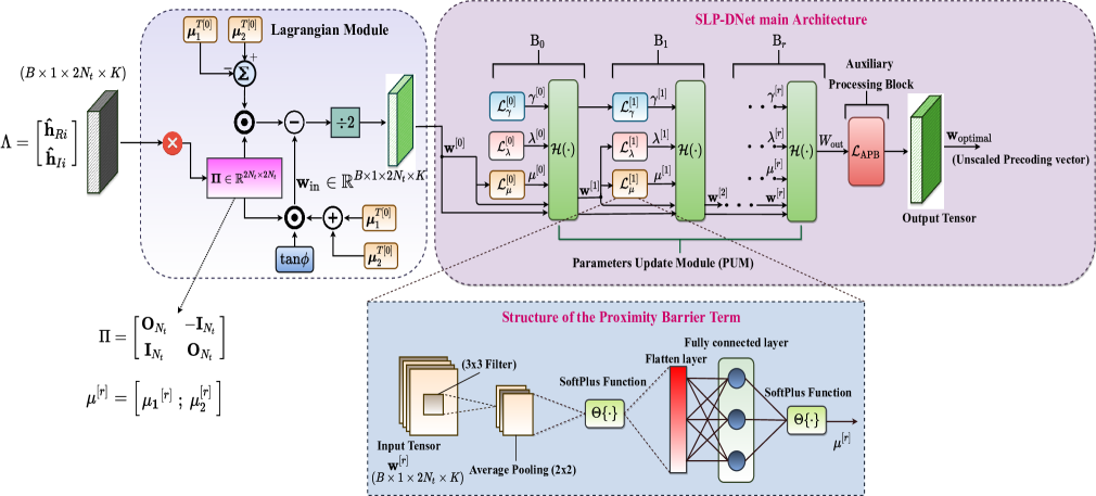
To build the proposed learning-based SLP architecture, we combine an IPM with a proximal forward-backward procedure as shown in Algorithm 1 and transform it into an NN structure represented by the proximity barrier term (see Fig. 2). The learning architecture strictly follows the formulation (28). We show a striking similarity between our proposal and the feed-forward. Intuitively, we form cascade layers of NN from (28) as follows

𝐰1[r+1]=proxγ[r]μ[r]B[(𝐈Nt2γ[r])𝐰1[r]+γ[r]λ[r]1T].superscriptsubscript𝐰1delimited-[]𝑟1subscriptproxsuperscript𝛾delimited-[]𝑟superscript𝜇delimited-[]𝑟𝐵delimited-[]subscript𝐈subscript𝑁𝑡2superscript𝛾delimited-[]𝑟superscriptsubscript𝐰1delimited-[]𝑟superscript𝛾delimited-[]𝑟superscript𝜆delimited-[]𝑟superscript1𝑇\mathbf{w}_{1}^{[r+1]}=\text{prox}_{\gamma^{[r]}{\mu}^{[r]}{B}}\left[\left(\mathbf{I}_{N_{t}}-2\gamma^{[r]}\right)\mathbf{w}_{1}^{[r]}+\gamma^{[r]}\lambda^{[r]}\textbf{1}^{T}\right]. (30)

where 11×2Nt1superscript12subscript𝑁𝑡\textbf{1}\in\mathbb{R}^{1\times 2N_{t}} is a vector of ones. By letting 𝐖r=𝐈2Nt2γ[r]subscript𝐖𝑟subscript𝐈2subscript𝑁𝑡2superscript𝛾delimited-[]𝑟\mathbf{W}_{r}=\mathbf{I}_{2N_{t}}-2\gamma^{[r]}, 𝐛r=γ[r]λ[r]1Tsubscript𝐛𝑟superscript𝛾delimited-[]𝑟superscript𝜆delimited-[]𝑟superscript1𝑇\mathbf{b}_{r}=\gamma^{[r]}\lambda^{[r]}\textbf{1}^{T} and 𝚯r=proxγ[r]μ[r]Bsubscript𝚯𝑟subscriptproxsuperscript𝛾delimited-[]𝑟superscript𝜇delimited-[]𝑟𝐵\bm{\Theta}_{r}=\text{prox}_{\gamma^{[r]}{\mu}^{[r]}{B}}, the r-layer network [r1][0]superscriptdelimited-[]𝑟1superscriptdelimited-[]0\mathcal{L}^{[r-1]}\cdots\mathcal{L}^{[0]} will correspond to the following

𝚯0(𝐖0+𝐛0),,𝚯r(𝐖r+𝐛r)subscript𝚯0subscript𝐖0subscript𝐛0subscript𝚯𝑟subscript𝐖𝑟subscript𝐛𝑟\bm{\Theta}_{0}\left(\mathbf{W}_{0}+\mathbf{b}_{0}\right),\cdots,\bm{\Theta}_{r}\left(\mathbf{W}_{r}+\mathbf{b}_{r}\right) (31)

where 𝐖rsubscript𝐖𝑟\mathbf{W}_{r} and 𝐛rsubscript𝐛𝑟\mathbf{b}_{r} are described as weight and bias parameters respectively. The nonlinear activation functions are defined by 𝚯rsubscript𝚯𝑟\bm{\Theta}_{r}.

In the SLP-DNet design, the Lagrange multiplier associated with the equality constraint is wired across the network to provide additional flexibility. It is important to note that the architectures are the same for both non-robust and robust power minimization problems described in Sections III and IV but differ in proximity barrier functions (PBFs). Therefore, to simplify our exposition, we build the structure of the learning framework based on (28) and the DU framework described in [33], which gives rise to Algorithm 1.

Algorithm 1 Feed-forward-Backward Proximal IPM
0:  𝐰1[0]superscriptsubscript𝐰1delimited-[]0\mathbf{w}_{1}^{[0]}, γ[0]superscript𝛾delimited-[]0{\gamma}^{[0]}, λ[0]superscript𝜆delimited-[]0{\lambda}^{[0]} and μ[0]superscript𝜇delimited-[]0{\mu}^{[0]}
0:  𝐰1subscript𝐰1\mathbf{w}_{1} Initialization :
1:  randomly initialize 𝐰1[0]2Nt×1superscriptsubscript𝐰1delimited-[]0superscript2subscript𝑁𝑡1\mathbf{w}_{1}^{[0]}\in{\mathbb{R}^{2N_{t}\times 1}}, μ[0]>0superscript𝜇delimited-[]00{\mu}^{[0]}>0, λ[0]>0superscript𝜆delimited-[]00\lambda^{[0]}>0 and γ[0]>0superscript𝛾delimited-[]00\gamma^{[0]}>0 i=1,,Kfor-all𝑖1𝐾\forall\ {i}=1,\ \cdots,\ K
2:  for r=0𝑟0r=0 to L𝐿L do
3:     𝐰1[r+1]=proxγ[r]μ[r]B(𝐰1[r]γ[r]ΔD(𝐰1[r],λ[r])).superscriptsubscript𝐰1delimited-[]𝑟1subscriptproxsuperscript𝛾delimited-[]𝑟superscript𝜇delimited-[]𝑟𝐵superscriptsubscript𝐰1delimited-[]𝑟superscript𝛾delimited-[]𝑟Δ𝐷superscriptsubscript𝐰1delimited-[]𝑟superscript𝜆delimited-[]𝑟\mathbf{w}_{1}^{[r+1]}=\text{prox}_{\gamma^{[r]}{\mu}^{[r]}B}\left(\mathbf{w}_{1}^{[r]}-\gamma^{[r]}\Delta{{D}(\mathbf{w}_{1}^{[r]},\ \lambda^{[r]})}\right).
4:  end for
5:  return  𝐰1subscript𝐰1\mathbf{w}_{1}
Algorithm 2 Proximity Barrier Operator of a Nonrobust SLP-DNet
0:  𝐡Risubscript𝐡𝑅𝑖\mathbf{h}_{Ri}, 𝐡Iisubscript𝐡𝐼𝑖\mathbf{h}_{Ii}, ΓisubscriptΓ𝑖\Gamma_{i} and w0(noise power)subscript𝑤0noise power{w}_{0}\ (\text{noise power})
0:  𝐰1subscript𝐰1\mathbf{w}_{1}, γ𝛾\gamma, μ𝜇{\mu} and λ𝜆\lambda Initialization :
1:  randomly initialize 𝐰02Nt×1subscript𝐰0superscript2subscript𝑁𝑡1\mathbf{w}_{0}\in{\mathbb{R}^{2N_{t}\times 1}}, μ[0]>0superscript𝜇delimited-[]00{\mu}^{[0]}>0, λ[0]>0superscript𝜆delimited-[]00\lambda^{[0]}>0 and γ[0]>0superscript𝛾delimited-[]00\gamma^{[0]}>0 i=1,,Kfor-all𝑖1𝐾\forall\ {i}=1,\ \cdots,\ K.
2:  Find the solution to (23) using Cardano formula.
3:  For every solution in step 2, compute its corresponding Barrier function using (21).
4:  Compute the Proximity Operator of the Barrier at 𝐰0subscript𝐰0\mathbf{w}_{0} using (15), where Φ(𝐰1,γ,μ)=proxγμB(𝐰1).Φsubscript𝐰1𝛾𝜇subscriptprox𝛾𝜇𝐵subscript𝐰1\Phi(\mathbf{w}_{1},\ \gamma,{\mu})=\text{prox}_{\gamma{\mu}{{B}}}{(\mathbf{w}_{1})}.
5:  Compute the derivatives of the Proximity Operator w.r.t 𝐰1subscript𝐰1\mathbf{w}_{1}, μ𝜇{\mu} and γ𝛾\gamma using (24), (25) and (26).
6:  Update the training variables as follows:
  1. (a)

    μ[r+1]=μ[r]ηΦ(𝐰1[r],γ[r],μ[r])μ[r]superscript𝜇delimited-[]𝑟1superscript𝜇delimited-[]𝑟𝜂Φsuperscriptsubscript𝐰1delimited-[]𝑟superscript𝛾delimited-[]𝑟superscript𝜇delimited-[]𝑟superscript𝜇delimited-[]𝑟{\mu}^{[r+1]}={\mu}^{[r]}-\eta\frac{\partial{\Phi}(\mathbf{w}_{1}^{[r]},\ \gamma^{[r]},\ {\mu}^{[r]})}{\partial{{\mu}^{[r]}}}

  2. (b)

    γ[r+1]=γ[r]ηΦ(𝐰1[r],γ[r],μ[r])γ[r]superscript𝛾delimited-[]𝑟1superscript𝛾delimited-[]𝑟𝜂Φsuperscriptsubscript𝐰1delimited-[]𝑟superscript𝛾delimited-[]𝑟superscript𝜇delimited-[]𝑟superscript𝛾delimited-[]𝑟\gamma^{[r+1]}=\gamma^{[r]}-\eta\frac{\partial{\Phi}(\mathbf{w}_{1}^{[r]},\ \gamma^{[r]},\ {\mu}^{[r]})}{\partial{\gamma^{[r]}}}

  3. (c)

    λ[r+1]=λ[r]ηD(𝐰1[r],λ[r])λ[r]superscript𝜆delimited-[]𝑟1superscript𝜆delimited-[]𝑟𝜂𝐷superscriptsubscript𝐰1delimited-[]𝑟superscript𝜆delimited-[]𝑟superscript𝜆delimited-[]𝑟\lambda^{[r+1]}=\lambda^{[r]}-\eta\frac{\partial{{D}(\mathbf{w}_{1}^{[r]},\ \lambda^{[r]})}}{\partial{\lambda^{[r]}}} using (29)

where η𝜂\eta is the learning rate.
7:  Use the results in step 6 and the Algorithm 1 to obtain the optimal precoding tensor.

As shown in Fig. 2, SLP-DNet has two main units; the parameter update module (PUM) and the auxiliary processing block (APB). The PUM has three core components associated with Lagrangian multipliers (equality and inequality constraints) and the training step-size, which are updated according to the following

(𝐰1,μ,γ,λ)=proxγ[r]μ[r]B(𝐰1[r]γ[r]ΔD(𝐰1[r],λ[r])).subscript𝐰1𝜇𝛾𝜆subscriptproxsuperscript𝛾delimited-[]𝑟superscript𝜇delimited-[]𝑟𝐵superscriptsubscript𝐰1delimited-[]𝑟superscript𝛾delimited-[]𝑟Δ𝐷superscriptsubscript𝐰1delimited-[]𝑟superscript𝜆delimited-[]𝑟\mathcal{H}(\mathbf{w}_{1},{\mu},\gamma,\lambda)=\text{prox}_{\gamma^{[r]}{\mu}^{[r]}B}\left(\mathbf{w}_{1}^{[r]}-\gamma^{[r]}\Delta{{D}(\mathbf{w}_{1}^{[r]},\lambda^{[r]})}\right). (32)

Furthermore, the component that forms the barrier term is constructed with one convolutional layer, an average pooling layer, a fully connected layer, and a Softplus layer to curb the output to a positive real value to satisfy the inequality constraint. The APB unit is connected to the last r-th block of the PUM in the form of a deep CNN to convert the output of the last parameter update block into a target transmit precoding vector. The APB architecture is made up of 3 convolution layers and 2 activation layers. In addition, a Batch Normalization layer is added between each convolutional layer and the activation layer to stabilize the mismatch in the distribution of the inputs caused by the internal covariate shift [37]. For every r block (r-th layer), there are three core components; μ[r]superscriptsubscript𝜇delimited-[]𝑟\mathcal{L}_{{\mu}}^{[r]}, γ[r]superscriptsubscript𝛾delimited-[]𝑟\mathcal{L}_{\gamma}^{[r]} and λ[r]superscriptsubscript𝜆delimited-[]𝑟\mathcal{L}_{\lambda}^{[r]} associated with the learnable parameters (μ𝜇{\mu}, γ𝛾\gamma and λ𝜆\lambda), respectively as shown in Fig. 2. These components form a learning block for computing the barrier parameter (μ𝜇{\mu}) associated with the inequality constraint, the step-size (γ𝛾\gamma) and the equality constraint (λ𝜆\lambda), if exists. To ensure that the constraints remain positive, a Softplus-sign function [38], Softplus(z)=ln(1+exp(z))Softplus𝑧1exp𝑧\text{Softplus}(z)=\ln{(1+\text{exp}(z))} is used.

Refer to caption
Figure 2: Complete SLP-DNet Architecture, showing the parameter update mouule, the auxiliary processing block.

The Softplus-sign function is a smooth approximation of the rectified linear unit (ReLu) activation function; and unlike the ReLu its gradient is never exactly equal to zero [38], which imposes an update on γ𝛾\gamma, μ𝜇{\mu} and λ𝜆\lambda during the backward propagation. The PBF for nonrobust SLP formulation is summarized in Algorithm 2 below. A similar algorithm can also be adopted for a robust PBF using a robust formulation. Finally, the output from the auxiliary processing block is the precoding vector in the real domain. The relation: 𝐰1=[𝐰R𝐰I]Tsubscript𝐰1superscriptdelimited-[]subscript𝐰𝑅subscript𝐰𝐼𝑇\mathbf{w}_{1}=[\mathbf{w}_{R}\ -\mathbf{w}_{I}]^{T} is used to convert it to its equivalent complex domain for every SINR value of the i-th user.

III-C1 Duality and Loss Function of the SLP Formulation

In order to ease the formulation of the dual-problem of the original problem (11), the left-hand-side of the inequality constraint is split into its equivalent positive and negative parts as follows

min{𝐰𝟏}subscript𝐰1min\displaystyle\underset{\mathbf{\{w_{1}\}}}{\text{min}} 𝐰122superscriptsubscriptdelimited-∥∥subscript𝐰122\displaystyle{\left\lVert\mathbf{w}_{1}\right\rVert_{2}^{2}} (33)
s.t. 𝚲iT𝚷𝐰1(𝚲iT𝚷𝐰1Γiv0)tanϕ,isuperscriptsubscript𝚲𝑖𝑇𝚷subscript𝐰1superscriptsubscript𝚲𝑖𝑇𝚷subscript𝐰1subscriptΓ𝑖subscript𝑣0tanitalic-ϕfor-all𝑖\displaystyle\bm{\Lambda}_{i}^{T}\bm{\Pi}\mathbf{w}_{1}\leq\left(\bm{\Lambda}_{i}^{T}\bm{\Pi}\mathbf{w}_{1}-\sqrt{\Gamma_{i}v_{0}}\right){\text{tan}{\phi}},\ \forall{i}
𝚲iT𝚷𝐰1(𝚲iT𝚷𝐰1Γiv0)tanϕ,i.superscriptsubscript𝚲𝑖𝑇𝚷subscript𝐰1superscriptsubscript𝚲𝑖𝑇𝚷subscript𝐰1subscriptΓ𝑖subscript𝑣0tanitalic-ϕfor-all𝑖\displaystyle-\bm{\Lambda}_{i}^{T}\bm{\Pi}\mathbf{w}_{1}\leq\left(\bm{\Lambda}_{i}^{T}\bm{\Pi}\mathbf{w}_{1}-\sqrt{\Gamma_{i}v_{0}}\right){\text{tan}{\phi}},\ \forall{i}.

The Lagrangian of (33) is defined as

rl(𝐰1,𝝁1,𝝁2)=𝐰122+𝝁1(𝚲iT𝚷𝐰1𝚲iT𝐰1tanϕ+Γiv0)𝝁2(𝚲iT𝚷𝐰1+𝚲iT𝐰1tanϕΓiv0),subscriptrlsubscript𝐰1subscript𝝁1subscript𝝁2superscriptsubscriptdelimited-∥∥subscript𝐰122subscript𝝁1subscriptsuperscript𝚲𝑇𝑖𝚷subscript𝐰1superscriptsubscript𝚲𝑖𝑇subscript𝐰1tanitalic-ϕsubscriptΓ𝑖subscript𝑣0subscript𝝁2subscriptsuperscript𝚲𝑇𝑖𝚷subscript𝐰1superscriptsubscript𝚲𝑖𝑇subscript𝐰1tanitalic-ϕsubscriptΓ𝑖subscript𝑣0\mathcal{L}_{\text{rl}}(\mathbf{w}_{1},\ \bm{\mu}_{1},\ \bm{\mu}_{2})=\left\lVert\mathbf{w}_{1}\right\rVert_{2}^{2}\\ +\bm{\mu}_{1}\left(\bm{\Lambda}^{T}_{i}\bm{\Pi}\mathbf{w}_{1}-\bm{\Lambda}_{i}^{T}\mathbf{w}_{1}\text{tan}{\phi}+\sqrt{\Gamma_{i}v_{0}}\right)\\ -\bm{\mu}_{2}\left(\bm{\Lambda}^{T}_{i}\bm{\Pi}\mathbf{w}_{1}+\bm{\Lambda}_{i}^{T}\mathbf{w}_{1}\text{tan}{\phi}-\sqrt{\Gamma_{i}v_{0}}\right), (34)

where 𝝁1subscript𝝁1\bm{\mu}_{1} and 𝝁2subscript𝝁2\bm{\mu}_{2} are the Lagrangian multipliers associated with the constraints and are related to the proximity barrier. The subscript ‘rl’ stands for relaxed phase rotation. It can be easily proven that the lower bound (LB) of (34) is \mathbcalLrl(𝐰1,𝝁1,𝝁2)𝝁1Λi(Πtanϕ)𝝁2Λi(Π+tanϕ)\mathbcalsubscript𝐿rlsubscript𝐰1subscript𝝁1subscript𝝁2subscript𝝁1subscriptΛ𝑖Πtanitalic-ϕsubscript𝝁2subscriptΛ𝑖Πtanitalic-ϕ\mathbcal{L}_{\text{rl}}(\mathbf{w}_{1},\bm{\mu}_{1},\bm{\mu}_{2})\geq\bm{\mu}_{1}\Lambda_{i}\left(\Pi-\text{tan}{\phi}\right)-\bm{\mu}_{2}\Lambda_{i}\left(\Pi+\text{tan}{\phi}\right). From (34), the optimal precoder is obtained by differentiating rl()subscriptrl\mathcal{L}_{\text{rl}}(\cdotp) w.r.t 𝐰1subscript𝐰1\mathbf{w}_{1} and equating to zero. By doing so, the optimal precoder can be found as

𝐰1=(𝝁𝟏T+𝝁𝟐T)𝚲itanϕ(𝝁𝟏T𝝁𝟐T)𝚷𝑻𝚲i2.subscript𝐰1superscriptsubscript𝝁1𝑇superscriptsubscript𝝁2𝑇subscript𝚲𝑖tanitalic-ϕsuperscriptsubscript𝝁1𝑇superscriptsubscript𝝁2𝑇superscript𝚷𝑻subscript𝚲𝑖2\mathbf{w}_{1}=\frac{\left(\bm{\mu_{1}}^{T}+\bm{\mu_{2}}^{T}\right)\cdotp\bm{\Lambda}_{i}\text{tan}{\phi}-\left(\bm{\mu_{1}}^{T}-\bm{\mu_{2}}^{T}\right)\cdotp\bm{\Pi^{T}}\bm{\Lambda}_{i}}{2}. (35)

In the sequel, we show that (35) is used to generate the training input (precoding vector) by randomly initializing the Lagrangian multipliers (𝝁1subscript𝝁1\bm{\mu}_{1} and 𝝁2subscript𝝁2\bm{\mu}_{2}) and then train the network to learn their values that minimize the loss function (Lagrangian function). The loss function is modified by adding \mathbcall2\mathbcalsubscript𝑙2\mathbcal{l}_{2}-norm regularization over the weights to calibrate the learning coefficients in order to adjust the learning process. It should be noted that the regularization here is not aimed at addressing the problem of overfitting as in the case of supervised learning. However, regularization in an unsupervised learning is used to normalize and moderate weights attached to a neuron to help stabilize the learning algorithm [39]. The loss function (34) over N𝑁N training samples is thus expressed as

rl(𝐰1,𝝁1,𝝁2)=1Ni=1N𝐰122+1Ni=1N(𝝁1(𝚲iT𝚷𝐰1𝚲iT𝐰1tanϕ+Γiv0))1Ni=1N(𝝁2(𝚲iT𝚷𝐰1+𝚲iT𝐰1tanϕΓiv0))+ϑNLi=1Ni=1L𝜽i22,subscriptrlsubscript𝐰1subscript𝝁1subscript𝝁21𝑁subscriptsuperscript𝑁𝑖1superscriptsubscriptdelimited-∥∥subscript𝐰1221𝑁subscriptsuperscript𝑁𝑖1subscript𝝁1subscriptsuperscript𝚲𝑇𝑖𝚷subscript𝐰1superscriptsubscript𝚲𝑖𝑇subscript𝐰1tanitalic-ϕsubscriptΓ𝑖subscript𝑣01𝑁subscriptsuperscript𝑁𝑖1subscript𝝁2subscriptsuperscript𝚲𝑇𝑖𝚷subscript𝐰1superscriptsubscript𝚲𝑖𝑇subscript𝐰1tanitalic-ϕsubscriptΓ𝑖subscript𝑣0italic-ϑ𝑁𝐿subscriptsuperscript𝑁𝑖1superscriptsubscript𝑖1𝐿superscriptsubscriptdelimited-∥∥subscript𝜽𝑖22\mathcal{L}_{\text{rl}}(\mathbf{w}_{1},\ \bm{\mu}_{1},\ \bm{\mu}_{2})=\frac{1}{N}\sum^{N}_{i=1}\|\mathbf{w}_{1}\|_{2}^{2}\\ +\frac{1}{N}\sum^{N}_{i=1}\left(\bm{\mu}_{1}\left(\bm{\Lambda}^{T}_{i}\bm{\Pi}\mathbf{w}_{1}-\bm{\Lambda}_{i}^{T}\mathbf{w}_{1}\text{tan}{\phi}+\sqrt{\Gamma_{i}v_{0}}\right)\right)\\ -\frac{1}{N}\sum^{N}_{i=1}\left(\bm{\mu}_{2}\left(\bm{\Lambda}^{T}_{i}\bm{\Pi}\mathbf{w}_{1}+\bm{\Lambda}_{i}^{T}\mathbf{w}_{1}\text{tan}{\phi}-\sqrt{\Gamma_{i}v_{0}}\right)\right)\\ +\frac{\vartheta}{NL}\sum^{N}_{i=1}\sum_{i=1}^{L}\|\bm{\theta}_{i}\|_{2}^{2}, (36)

where 𝜽isubscript𝜽𝑖\bm{\theta}_{i} are the trainable parameters of the i-th layers associated with the weights and biases, and ϑ>0italic-ϑ0\vartheta>0 is the penalty parameter that controls the bias and variance of the trainable coefficients, N𝑁N, L𝐿L is the number of training samples (batch size or the number of channel realization) and the number of layers, respectively.

III-D Learning-Based SLP for Strict Angle Rotation

In the previous subsection, we have presented SLP-DNet based on relaxed angle formulation. In this subsection, we provide a formulation for strict phase angle rotation where all the interfering signals align exactly to the phase the signal of interest (i.e. ϕ=0italic-ϕ0\phi=0 in Fig. 1), the optimization problem is [2]

min{𝐰𝟏}subscript𝐰1min\displaystyle\underset{\mathbf{\{w_{1}\}}}{\text{min}} 𝐰12superscriptdelimited-∥∥subscript𝐰12\displaystyle{\left\lVert\mathbf{w}_{1}\right\rVert^{2}} (37)
s.t. 𝚲iT𝚷𝐰1=0,isuperscriptsubscript𝚲𝑖𝑇𝚷subscript𝐰10for-all𝑖\displaystyle{\bm{\Lambda}_{i}^{T}\bm{\Pi}\mathbf{w}_{1}=0}\ ,\ \forall{i}
𝚲iT𝐰1Γiv0,i.superscriptsubscript𝚲𝑖𝑇subscript𝐰1subscriptΓ𝑖subscript𝑣0for-all𝑖\displaystyle\bm{\Lambda}_{i}^{T}\mathbf{w}_{1}\geq\sqrt{\Gamma_{i}v_{0}}\ ,\ \forall{i}.

We observe that the inequality constraint in (37) is affine. Based on this, the proximal barrier function for the strict phase rotation is

Bst(𝐰1)={ln(𝚲iT𝐰1Γiv0),if𝚲iT𝐰1Γiv0+,otherwise.B_{\text{st}}(\mathbf{w}_{1})=\left\{\begin{aligned} &-\ln{\left(\bm{\Lambda}_{i}^{T}\mathbf{w}_{1}-\sqrt{{\Gamma}_{i}v_{0}}\right)},&&\text{if}\ \bm{\Lambda}_{i}^{T}\mathbf{w}_{1}\geq\sqrt{{\Gamma}_{i}v_{0}}\\ &+\infty,&&\text{otherwise.}\end{aligned}\right. (38)

The subscript ‘st’ represents strict phase rotation. Therefore, for every precoding vector 𝐰12Nt×1subscript𝐰1superscript2subscript𝑁𝑡1\mathbf{w}_{1}\in\mathbb{R}^{2N_{t}\times 1}, the proximity operator of μγBst𝜇𝛾subscript𝐵st{\mu}\gamma{B}_{\text{st}} at 𝐰1subscript𝐰1\mathbf{w}_{1} is given by

Φst(𝐰1,μ,γ)=𝐰1+𝚲𝒊T𝐰1Γiv0(𝚲iT𝐰1Γiv0)2+4γμ𝚲iT222𝚲i22𝚲i.subscriptΦstsubscript𝐰1𝜇𝛾subscript𝐰1superscriptsubscript𝚲𝒊𝑇subscript𝐰1subscriptΓ𝑖subscript𝑣0superscriptsuperscriptsubscript𝚲𝑖𝑇subscript𝐰1subscriptΓ𝑖subscript𝑣024𝛾𝜇superscriptsubscriptdelimited-∥∥superscriptsubscript𝚲𝑖𝑇222superscriptsubscriptdelimited-∥∥subscript𝚲𝑖22subscript𝚲𝑖\Phi_{\text{st}}(\mathbf{w}_{1},{\mu},\gamma)=\mathbf{w}_{1}+\\ \frac{\bm{\Lambda_{i}}^{T}\mathbf{w}_{1}-\sqrt{\Gamma_{i}v_{0}}-\sqrt{(\bm{\Lambda}_{i}^{T}\mathbf{w}_{1}-\sqrt{\Gamma_{i}v_{0}})^{2}+4\gamma{\mu}\left\lVert\bm{\Lambda}_{i}^{T}\right\rVert_{2}^{2}}}{{{2\left\lVert\bm{\Lambda}_{i}\right\rVert_{2}^{2}}}}\bm{\Lambda}_{i}. (39)

Similar to the steps in subsection III-B, the learning-based framework for SLP strict phase rotation is designed by finding the Jacobian matrix of Φ(𝐰1,μ,γ)Φsubscript𝐰1𝜇𝛾\Phi(\mathbf{w}_{1},{\mu},\gamma) with respect to 𝐰1subscript𝐰1\mathbf{w}_{1}, and the derivatives of Φ(𝐰1,μ,γ)Φsubscript𝐰1𝜇𝛾\Phi(\mathbf{w}_{1},{\mu},\gamma) with respect to γ𝛾\gamma and μ𝜇\mu can be easily obtained from (39). The loss function over N𝑁N training batches is given by

st(𝐰1,𝝀,𝝁)=1Ni=1N(𝐰122+𝝀𝚲iT𝚷𝐯1)+1Ni=1N(𝝁(Γiv0𝚲iT𝐰1))+ϑNLi=1Ni=1L𝜽i22,subscriptstsubscript𝐰1𝝀𝝁1𝑁subscriptsuperscript𝑁𝑖1superscriptsubscriptdelimited-∥∥subscript𝐰122𝝀subscriptsuperscript𝚲𝑇𝑖𝚷subscript𝐯11𝑁subscriptsuperscript𝑁𝑖1𝝁subscriptΓ𝑖subscript𝑣0subscriptsuperscript𝚲𝑇𝑖subscript𝐰1italic-ϑ𝑁𝐿subscriptsuperscript𝑁𝑖1superscriptsubscript𝑖1𝐿superscriptsubscriptdelimited-∥∥subscript𝜽𝑖22\mathcal{L}_{\text{st}}(\mathbf{w}_{1},\bm{\lambda},\ \bm{\mu})=\frac{1}{N}\sum^{N}_{i=1}\left(\|\mathbf{w}_{1}\|_{2}^{2}+\bm{\lambda}\bm{\Lambda}^{T}_{i}\bm{\Pi}\mathbf{v}_{1}\right)+\\ \frac{1}{N}\sum^{N}_{i=1}\left(\bm{\mu}\left(\sqrt{\Gamma_{i}v_{0}}-\bm{\Lambda}^{T}_{i}\mathbf{w}_{1}\right)\right)+\frac{\vartheta}{NL}\sum^{N}_{i=1}\sum_{i=1}^{L}\|\bm{\theta}_{i}\|_{2}^{2}, (40)

where 𝝁𝝁\bm{\mu} and 𝝀𝝀\bm{\lambda} are the Lagrangian multipliers for inequality and equality constraints, respectively. Finally, minimizing (40) with respect to 𝐰1subscript𝐰1\mathbf{w}_{1} (differentiating st()subscriptst\mathcal{L}_{\text{st}}(\cdotp) w.r.t 𝐰1subscript𝐰1\mathbf{w}_{1}), gives the optimal precoder as

𝐰1=𝝁T𝚲i𝝀T𝚷𝚲i2.subscript𝐰1superscript𝝁𝑇subscript𝚲𝑖superscript𝝀𝑇𝚷subscript𝚲𝑖2\mathbf{w}_{1}=\frac{\bm{\mu}^{T}\cdotp\bm{\Lambda}_{i}-\bm{\lambda}^{T}\cdotp\bm{\Pi}\bm{\Lambda}_{i}}{2}. (41)

IV Learning-Based Robust Power Minimization SLP with Channel Uncertainty

IV-A Channel Uncertainty and Channel error Model

So far, we have derived the unsupervised learning scheme in which the uncertainty in estimating the channel coefficients is not considered. The exact CSI is often unobtainable in practice. To model the user’s actual channel in the uncertainty region, we consider an ellipsoid ξ𝜉\xi such that

𝐡^i=𝐡¯i+𝒆¯ik,subscript^𝐡𝑖subscript¯𝐡𝑖subscript¯𝒆𝑖for-all𝑘\hat{\mathbf{h}}_{i}=\bar{\mathbf{h}}_{i}+\bar{\bm{e}}_{i}\ \forall{k}, (42)

where 𝐡¯isubscript¯𝐡𝑖\bar{\mathbf{h}}_{i} is the known CSI estimates at the BS and 𝒆¯isubscript¯𝒆𝑖\bar{\bm{e}}_{i} denotes the channel error within the uncertainty region of the ellipsoid (i.e 𝐡^iξsubscript^𝐡𝑖𝜉\hat{\mathbf{h}}_{i}\in\xi). The model of the uncertainty ellipsoid with the center 𝐡¯isubscript¯𝐡𝑖\bar{\mathbf{h}}_{i} is expressed as

ξ={𝐡¯i+𝐞¯i|𝐞¯i1}.\xi=\left\{\bar{\mathbf{h}}_{i}+\bar{\mathbf{e}}_{i}|_{\|\bar{\mathbf{e}}_{i}\leq 1\|}\right\}. (43)

As shown in [2], the channel error is given by {𝐞¯i:𝐞¯i22ςi2}conditional-setsubscript¯𝐞𝑖superscriptsubscriptdelimited-∥∥subscript¯𝐞𝑖22subscriptsuperscript𝜍2𝑖\left\{\bar{\mathbf{e}}_{i}:\left\lVert\bar{\mathbf{e}}_{i}\right\rVert_{2}^{2}\leq{\varsigma}^{2}_{i}\right\}. It is important to note that the BS is assumed to have the knowledge about the channel error, excluding its corresponding error bound ςi2subscriptsuperscript𝜍2𝑖{\varsigma}^{2}_{i}. For details and formulation of the conventional robust BLP, we refer the reader to [40].

IV-B Robust Optimization-Based SLP Formulation

The multi-cast constructive interference formulation of the power minimization problem for the worst-case CSI error is given by [40]

min{𝐰}𝐰min\displaystyle\underset{\mathbf{\{w\}}}{\text{min}} 𝐰22superscriptsubscriptdelimited-∥∥𝐰22\displaystyle{\left\lVert\mathbf{w}\right\rVert_{2}^{2}} (44)
s.t. |Im(𝐡^iT𝐰)|(Re(𝐡^iT𝐰)Γiv0)tanϕ0,\displaystyle\Bigl{|}{\text{Im}\left(\hat{\mathbf{h}}_{i}^{T}\mathbf{w}\right)\Bigl{|}}-\left({\text{Re}\left(\hat{\mathbf{h}}_{i}^{T}\mathbf{w}\right)}-\sqrt{\Gamma_{i}v_{0}}\right)\text{tan}{\phi}\leq 0,
𝐞¯i2ςi2,i.for-allsuperscriptdelimited-∥∥subscript¯𝐞𝑖2superscriptsubscript𝜍𝑖2for-all𝑖\displaystyle\forall\left\lVert\bar{\mathbf{e}}_{i}\right\rVert^{2}\leq{\varsigma}_{i}^{2},\ \forall{i}.

The intractability of the constraint in (44) can be effectively handled using convex optimization methods. Therefore, to guarantee that the robust constraint in (44) is satisfied, it is modified as follows [2]

maxe¯i2ςi2(|Im(𝐡^T𝐰)|(Re(𝐡^T𝐰)Γv0)tanϕ)0.\max_{\|\bar{e}_{i}\|^{2}\leq\varsigma^{2}_{i}}\left(\Bigl{|}\text{Im}\left(\hat{\mathbf{h}}^{T}\mathbf{w}\right)\Bigl{|}-\left(\text{Re}\left(\hat{\mathbf{h}}^{T}\mathbf{w}\right)-\sqrt{\Gamma v_{0}}\right)\text{tan}\phi\right)\leq 0. (45)

It is worth noting that the subscripts in (45) are ignored in order to simplify the problem formulation. By defining the equivalent real-valued channel and channel error vectors, the real and imaginary parts in the constraint can be decomposed into two separate constraints as explained in Section III (see (8a) and (8b)). Thus the robust formulation of the constraint is equivalent to two separate real-valued constraints as follows

𝚲T𝐰1𝚲T𝐰2tanϕ+ς𝐰1𝐰2tanϕ2+Γv0tanϕ0,superscript𝚲𝑇subscript𝐰1superscript𝚲𝑇subscript𝐰2tanitalic-ϕ𝜍subscriptdelimited-∥∥subscript𝐰1subscript𝐰2tanitalic-ϕ2Γsubscript𝑣0tanitalic-ϕ0\bm{\Lambda}^{T}\mathbf{w}_{1}-\bm{\Lambda}^{T}\mathbf{w}_{2}\text{tan}{\phi}+\varsigma\left\lVert\mathbf{w}_{1}-\mathbf{w}_{2}\text{tan}{\phi}\right\rVert_{2}+\sqrt{\Gamma v_{0}}\text{tan}\phi\leq 0, (46)
𝚲T𝐰1𝚲T𝐰2tanϕ+ς𝐰1+𝐰2tanϕ2+Γv0tanϕ0,superscript𝚲𝑇subscript𝐰1superscript𝚲𝑇subscript𝐰2tanitalic-ϕ𝜍subscriptdelimited-∥∥subscript𝐰1subscript𝐰2tanitalic-ϕ2Γsubscript𝑣0tanitalic-ϕ0-\bm{\Lambda}^{T}\mathbf{w}_{1}-\bm{\Lambda}^{T}\mathbf{w}_{2}\text{tan}{\phi}+\varsigma\left\lVert\mathbf{w}_{1}+\mathbf{w}_{2}\text{tan}{\phi}\right\rVert_{2}+\sqrt{\Gamma v_{0}}\text{tan}\phi\leq 0, (47)

where 𝚲=[𝐡¯R𝐡¯I]T𝚲superscriptmatrixsubscript¯𝐡𝑅subscript¯𝐡𝐼𝑇\bm{\Lambda}=\begin{bmatrix}\bar{\mathbf{h}}_{R}&\bar{\mathbf{h}}_{I}\end{bmatrix}^{T}, 𝐞=Δ[𝐞¯R𝐞¯I]T𝐞Δsuperscriptmatrixsubscript¯𝐞𝑅subscript¯𝐞𝐼𝑇\mathbf{e}\overset{\Delta}{=}\begin{bmatrix}\bar{\mathbf{e}}_{R}&\bar{\mathbf{e}}_{I}\end{bmatrix}^{T} and 𝐡^=𝐡¯R+j𝐡¯I+𝐞¯R+j𝐞¯I^𝐡subscript¯𝐡𝑅𝑗subscript¯𝐡𝐼subscript¯𝐞𝑅𝑗subscript¯𝐞𝐼\hat{\mathbf{h}}=\bar{\mathbf{h}}_{R}+j\bar{\mathbf{h}}_{I}+\bar{\mathbf{e}}_{R}+j\bar{\mathbf{e}}_{I}. Finally, the robust CI formulation for power minimization problem becomes

min{𝐰𝟏,𝐰𝟐}subscript𝐰1subscript𝐰2min\displaystyle\underset{\mathbf{\{w_{1},w_{2}\}}}{\text{min}} 𝐰122superscriptsubscriptdelimited-∥∥subscript𝐰122\displaystyle{\left\lVert\mathbf{w}_{1}\right\rVert_{2}^{2}} (48)
s.t. Constraints(46)and(47),iConstraints46and47for-all𝑖\displaystyle\text{Constraints}\ (\ref{robust_constraint1})\ \text{and}\ (\ref{robust_constraint2}),\ \forall{i}
where𝐰1=𝚷𝐰2.wheresubscript𝐰1𝚷subscript𝐰2\displaystyle\text{where}\ \ \mathbf{w}_{1}=\bm{\Pi}\mathbf{w}_{2}.

IV-C Proposed Unsupervised Learning-Based Robust SLP

In this subsection, we extend our proposed unsupervised learning formulation to a worst-case CSI-error to design a robust precoding scheme for the power minimization problem. As an extension of the previous formulations in subsection III-B, the focus here is to derive a PBF for the robust learning-based precoding scheme. Substituting for 𝐰1subscript𝐰1\mathbf{w}_{1} in (48), we have

(𝚲T𝚷𝚲Ttanϕ)𝐰2+ς(𝚷tanϕ)𝐰22+Γv0tanϕ0,superscript𝚲𝑇𝚷superscript𝚲𝑇tanitalic-ϕsubscript𝐰2𝜍subscriptdelimited-∥∥𝚷tanitalic-ϕsubscript𝐰22Γsubscript𝑣0tanitalic-ϕ0\left(\bm{\Lambda}^{T}\bm{\Pi}-\bm{\Lambda}^{T}\text{tan}{\phi}\right)\mathbf{w}_{2}+\varsigma\left\lVert\left(\bm{\Pi}-\text{tan}{\phi}\right)\mathbf{w}_{2}\right\rVert_{2}\\ +\sqrt{\Gamma v_{0}}\text{tan}\phi\leq 0, (49)
(𝚲T𝚷+𝚲Ttanϕ)𝐰2+ς(𝚷+tanϕ)𝐰22+Γv0tanϕ0.superscript𝚲𝑇𝚷superscript𝚲𝑇tanitalic-ϕsubscript𝐰2𝜍subscriptdelimited-∥∥𝚷tanitalic-ϕsubscript𝐰22Γsubscript𝑣0tanitalic-ϕ0-\left(\bm{\Lambda}^{T}\bm{\Pi}+\bm{\Lambda}^{T}\text{tan}{\phi}\right)\mathbf{w}_{2}+\varsigma\left\lVert\left(\bm{\Pi}+\text{tan}{\phi}\right)\mathbf{w}_{2}\right\rVert_{2}\\ +\sqrt{\Gamma v_{0}}\text{tan}\phi\leq 0. (50)

Apparently, the constraints (49) and (50) are bounded by the 𝓁2subscript𝓁2\mathcal{l}_{2}-norm. Therefore, problem (48) is rewritten as

min{𝐰𝟐}subscript𝐰2min\displaystyle\underset{\mathbf{\{w_{2}\}}}{\text{min}} 𝐰222superscriptsubscriptdelimited-∥∥subscript𝐰222\displaystyle{\left\lVert\mathbf{w}_{2}\right\rVert_{2}^{2}} (51)
s.t. Constraints(49)and(50),i.Constraints49and50for-all𝑖\displaystyle\text{Constraints}\ (\ref{robust_constraint12})\ \text{and}\ (\ref{robust_constraint22}),\ \forall{i}.

The resulting barrier function of the corresponding constraints of (51) is the sum of the individual barrier functions associated with the two inequality constraints. We begin by introducing the feasible set of solutions bounded by the Euclidean ball.

IV-C1 Bounded Euclidean ball Constraint

Suppose a problem whose set of feasible solutions is bounded by the Euclidean ball [41]

\mathbcalC={𝐳n|𝐳𝐱2β},\mathbcal𝐶conditional-set𝐳superscript𝑛subscriptdelimited-∥∥𝐳𝐱2𝛽\mathbcal{C}=\{\mathbf{z}\in\mathbb{R}^{n}\big{|}\left\lVert\mathbf{z}-\mathbf{x}\right\rVert_{2}\leq\beta\}, (52)

where β>0𝛽0\beta>0 and 𝐱n𝐱superscript𝑛\mathbf{x}\in\mathbb{R}^{n}. Let γ>0𝛾0\gamma>0 and μ>0𝜇0\mu>0 be the step-size and the Lagrange multiplier associated with the inequality constraint, respectively. Then the barrier function is expressed as [41]

B(𝐳)={ln(β𝐳𝐱2),if𝐳𝐱2<β,+,otherwise{B(\mathbf{z})}=\left\{\begin{aligned} &-\ln{\left(\beta-\left\lVert\mathbf{z}-\mathbf{x}\right\rVert_{2}\right)},&&\text{if}\ \left\lVert\mathbf{z}-\mathbf{x}\right\rVert_{2}<\beta,\\ &+\infty,&&\text{otherwise}\end{aligned}\right. (53)

For simplicity, we let 𝐐1=(𝚷𝐈2Nttanϕ)subscript𝐐1𝚷subscript𝐈2subscript𝑁𝑡tanitalic-ϕ\mathbf{Q}_{1}=\left(\bm{\Pi}-\mathbf{I}_{2N_{t}}\text{tan}{\phi}\right) and 𝐐2=(𝚷+𝐈2Nttanϕ)subscript𝐐2𝚷subscript𝐈2subscript𝑁𝑡tanitalic-ϕ\mathbf{Q}_{2}=\left(\bm{\Pi}+\mathbf{I}_{2N_{t}}\text{tan}{\phi}\right). Based on (53), the barrier function corresponding to the constraint (49) is written at the bottom of the page.


B1(𝐰2)={ln(Γv0tanϕ(𝚲T𝐐1𝐰2+ς𝐐1𝐰22)),if𝚲T𝐐1𝐰2+ς𝐐1𝐰22<Γv0tanϕ+otherwise{B_{1}(\mathbf{w}_{2})}=\left\{\begin{aligned} &-\ln{\left(-\sqrt{\Gamma v_{0}}\text{tan}{\phi}-\left(\bm{\Lambda}^{T}\mathbf{Q}_{1}\mathbf{w}_{2}+\varsigma\left\lVert\mathbf{Q}_{1}\mathbf{w}_{2}\right\rVert_{2}\right)\right)},&&\text{if}\ \bm{\Lambda}^{T}\mathbf{Q}_{1}\mathbf{w}_{2}+\varsigma\left\lVert\mathbf{Q}_{1}\mathbf{w}_{2}\right\rVert_{2}<-\sqrt{\Gamma v_{0}}\text{tan}{\phi}\\ &+\infty&&\text{otherwise}\end{aligned}\right. (54)

In the case of constraint (50), similar expression is also written for B2(𝐰2)subscript𝐵2subscript𝐰2{B_{2}(\mathbf{w}_{2})} using 𝐐2subscript𝐐2\mathbf{Q}_{2}. The resulting barrier function is thus

Brobust(𝐰2)=B1(𝐰2)+B2(𝐰2)subscript𝐵robustsubscript𝐰2subscript𝐵1subscript𝐰2subscript𝐵2subscript𝐰2{B}_{\text{robust}}(\mathbf{w}_{2})={B_{1}(\mathbf{w}_{2})}+{B_{2}(\mathbf{w}_{2})} (55)

Without loss of generality, the constraints (49) and (50) can be further written as

𝚲T𝐐1𝐰2+ς𝐐1𝐰22+Γv0tanϕ0,superscript𝚲𝑇subscript𝐐1subscript𝐰2𝜍subscriptdelimited-∥∥subscript𝐐1subscript𝐰22Γsubscript𝑣0tanitalic-ϕ0\bm{\Lambda}^{T}\mathbf{Q}_{1}\mathbf{w}_{2}+\varsigma\left\lVert\mathbf{Q}_{1}\mathbf{w}_{2}\right\rVert_{2}+\sqrt{\Gamma v_{0}}\text{tan}{\phi}\leq 0, (56)
𝚲T𝐐2𝐰2+ς𝐐2𝐰22+Γv0tanϕ0.superscript𝚲𝑇subscript𝐐2subscript𝐰2𝜍subscriptdelimited-∥∥subscript𝐐2subscript𝐰22Γsubscript𝑣0tanitalic-ϕ0\bm{\Lambda}^{T}\mathbf{Q}_{2}\mathbf{w}_{2}+\varsigma\left\lVert\mathbf{Q}_{2}\mathbf{w}_{2}\right\rVert_{2}+\sqrt{\Gamma v_{0}}\text{tan}{\phi}\leq 0. (57)

It can be seen that the upper bound of the two constraints (56) and (57) is zero, Therefore, the effective proximity operator of (55) is obtained the by squaring (56) and (57) and adding the results. Following similar steps presented in subsection III-B, we obtain the proximity operator of the barrier for the robust SLP-DNet (see Appendix A for details).

IV-C2 Loss Function of the Robust Power Minimization Problem

The training loss function is the Lagrangian of (51), and can be written as

min{𝐰𝟐}𝐰222s.t.𝚲T𝐐1𝐰2+ς𝐐1𝐰22+Γv0tanϕ0i𝚲T𝐐2𝐰2+ς𝐐2𝐰22+Γv0tanϕ0i.missing-subexpressionsubscript𝐰2minmissing-subexpressionsuperscriptsubscriptdelimited-∥∥subscript𝐰222missing-subexpressions.t.missing-subexpressionsuperscript𝚲𝑇subscript𝐐1subscript𝐰2𝜍subscriptdelimited-∥∥subscript𝐐1subscript𝐰22Γsubscript𝑣0tanitalic-ϕ0for-all𝑖missing-subexpressionmissing-subexpressionmissing-subexpressionsuperscript𝚲𝑇subscript𝐐2subscript𝐰2𝜍subscriptdelimited-∥∥subscript𝐐2subscript𝐰22Γsubscript𝑣0tanitalic-ϕ0for-all𝑖\begin{aligned} &\underset{\mathbf{\{w_{2}\}}}{\text{min}}&&{\left\lVert\mathbf{w}_{2}\right\rVert_{2}^{2}}\\ &\text{s.t.}&&\bm{\Lambda}^{T}\mathbf{Q}_{1}\mathbf{w}_{2}+\varsigma\left\lVert\mathbf{Q}_{1}\mathbf{w}_{2}\right\rVert_{2}+\sqrt{\Gamma v_{0}}\text{tan}{\phi}\leq 0\ \forall{i}\\ &&&\bm{\Lambda}^{T}\mathbf{Q}_{2}\mathbf{w}_{2}+\varsigma\left\lVert\mathbf{Q}_{2}\mathbf{w}_{2}\right\rVert_{2}+\sqrt{\Gamma v_{0}}\text{tan}{\phi}\leq 0\ \forall{i}.\end{aligned}

(58)

Therefore, the loss function of (58) is the regularized Lagrangian parameterized by 𝜽isubscript𝜽𝑖\bm{\theta}_{i} over the entire layers

robust(𝐰2,𝝁1,𝝁2)=1Ni=1N𝐰222+𝝁1Ni=1N(ς2𝐐1𝐰222(Γv0tanϕ𝚲T𝐐1𝐰2)2)+𝝁2Ni=1N(ς2𝐐2𝐰222(Γv0tanϕ𝚲T𝐐2𝐰2)2)+ϑNLi=1Ni=1L𝜽i22.subscriptrobustsubscript𝐰2subscript𝝁1subscript𝝁21𝑁subscriptsuperscript𝑁𝑖1superscriptsubscriptdelimited-∥∥subscript𝐰222subscript𝝁1𝑁subscriptsuperscript𝑁𝑖1superscript𝜍2superscriptsubscriptdelimited-∥∥subscript𝐐1subscript𝐰222superscriptΓsubscript𝑣0tanitalic-ϕsuperscript𝚲𝑇subscript𝐐1subscript𝐰22subscript𝝁2𝑁subscriptsuperscript𝑁𝑖1superscript𝜍2superscriptsubscriptdelimited-∥∥subscript𝐐2subscript𝐰222superscriptΓsubscript𝑣0tanitalic-ϕsuperscript𝚲𝑇subscript𝐐2subscript𝐰22italic-ϑ𝑁𝐿subscriptsuperscript𝑁𝑖1superscriptsubscript𝑖1𝐿superscriptsubscriptdelimited-∥∥subscript𝜽𝑖22\mathcal{L}_{\text{robust}}(\mathbf{w}_{2},\ \bm{\mu}_{1},\ \bm{\mu}_{2})=\frac{1}{N}\sum^{N}_{i=1}\|\mathbf{w}_{2}\|_{2}^{2}\\ +\frac{\bm{\mu}_{1}}{N}\sum^{N}_{i=1}\left({\varsigma}^{2}\left\lVert\mathbf{Q}_{1}\mathbf{w}_{2}\right\rVert_{2}^{2}-\left(\sqrt{\Gamma v_{0}}\text{tan}{\phi}-\bm{\Lambda}^{T}\mathbf{Q}_{1}\mathbf{w}_{2}\right)^{2}\right)\\ +\frac{\bm{\mu}_{2}}{N}\sum^{N}_{i=1}\left({\varsigma}^{2}\left\lVert\mathbf{Q}_{2}\mathbf{w}_{2}\right\rVert_{2}^{2}-\left(\sqrt{\Gamma v_{0}}\text{tan}{\phi}-\bm{\Lambda}^{T}\mathbf{Q}_{2}\mathbf{w}_{2}\right)^{2}\right)\\ +\frac{\vartheta}{NL}\sum^{N}_{i=1}\sum_{i=1}^{L}\|\bm{\theta}_{i}\|_{2}^{2}. (59)

The minimum of (59) with respect to 𝐰2subscript𝐰2\mathbf{w}_{2} by equating its derivative to zero

(1+(𝝁1𝐐122+𝝁2𝐐222)(ς2𝚲T𝚲))𝐰2=(𝝁1𝐐1+𝝁2𝐐2)𝚲Γv0tanϕ.1subscript𝝁1superscriptsubscriptdelimited-∥∥subscript𝐐122subscript𝝁2superscriptsubscriptdelimited-∥∥subscript𝐐222superscript𝜍2superscript𝚲𝑇𝚲subscript𝐰2subscript𝝁1subscript𝐐1subscript𝝁2subscript𝐐2𝚲Γsubscript𝑣0tanitalic-ϕ\left(1+\left(\bm{\mu}_{1}\left\lVert\mathbf{Q}_{1}\right\rVert_{2}^{2}+\bm{\mu}_{2}\left\lVert\mathbf{Q}_{2}\right\rVert_{2}^{2}\right)\left({\varsigma}^{2}-\bm{\Lambda}^{T}\bm{\Lambda}\right)\right){\mathbf{w}_{2}}=\\ -\left(\bm{\mu}_{1}\mathbf{Q}_{1}+\bm{\mu}_{2}\mathbf{Q}_{2}\right)\bm{\Lambda}\sqrt{\Gamma{v}_{0}\text{tan}{\phi}}. (60)

For convenience, we redefine the real matrices and vectors as [𝐐122𝐐222]=𝐪¯normmatrixsuperscriptsubscriptnormsubscript𝐐122superscriptsubscriptnormsubscript𝐐222subscript¯𝐪norm\begin{bmatrix}\|\mathbf{Q}_{1}\|_{2}^{2}&\|\mathbf{Q}_{2}\|_{2}^{2}\end{bmatrix}=\bar{\mathbf{q}}_{\text{norm}}; [𝐐1𝐐2]=𝐐¯matrixsubscript𝐐1subscript𝐐2¯𝐐\begin{bmatrix}\mathbf{Q}_{1}&\mathbf{Q}_{2}\end{bmatrix}=\bar{\mathbf{Q}} and [𝝁1𝝁2]=𝝁¯matrixsubscript𝝁1subscript𝝁2¯𝝁\begin{bmatrix}\bm{\mu}_{1}&\bm{\mu}_{2}\end{bmatrix}=\bar{\bm{\mu}}. With these new notations, (60) is simplified to

(𝐈2Nt+𝐪¯norm𝝁¯T(ς2𝚲𝑻𝚲))𝐰2=𝚲𝐐¯𝝁¯TΓw0tanϕsubscript𝐈2subscript𝑁𝑡subscript¯𝐪normsuperscriptbold-¯𝝁𝑇superscript𝜍2superscript𝚲𝑻𝚲subscript𝐰2𝚲¯𝐐superscriptbold-¯𝝁𝑇Γsubscript𝑤0tanitalic-ϕ\left(\mathbf{I}_{2N_{t}}+\mathbf{\bar{q}}_{\text{norm}}\bm{\bar{\mu}}^{T}\left({\varsigma}^{2}-\bm{\Lambda^{T}\Lambda}\right)\right){\mathbf{w}_{2}}=-\bm{\Lambda}\mathbf{\bar{Q}}{\bm{\bar{\mu}}}^{T}\sqrt{\Gamma{w}_{0}}{\text{tan}{\phi}} (61)

From (61), the optimal transmit precoder is thus

𝐰2=𝚲𝐐¯𝝁¯T𝐀1Γv0tanϕ,subscript𝐰2𝚲¯𝐐superscriptbold-¯𝝁𝑇superscript𝐀1Γsubscript𝑣0tanitalic-ϕ\mathbf{w}_{2}=-\bm{\Lambda}\mathbf{\bar{Q}}{\bm{\bar{\mu}}}^{T}{\mathbf{A}}^{-1}\sqrt{\Gamma{v}_{0}}{\text{tan}{\phi}}, (62)

where 𝐀=(𝐈2Nt+𝐪¯norm𝝁¯T(ς2𝚲𝑻𝚲))𝐀subscript𝐈2subscript𝑁𝑡subscript¯𝐪normsuperscriptbold-¯𝝁𝑇superscript𝜍2superscript𝚲𝑻𝚲{\mathbf{A}}=\left(\mathbf{I}_{2N_{t}}+\mathbf{\bar{q}}_{\text{norm}}\bm{\bar{\mu}}^{T}\left({\varsigma}^{2}-\bm{\Lambda^{T}\Lambda}\right)\right). Note that the Lagrange multipliers 𝝁1subscript𝝁1\bm{\mu}_{1} and 𝝁2subscript𝝁2\bm{\mu}_{2} are associated with the barrier term and are randomly initialized from a uniform distribution.

V Data Generation, Training and Computational Complexity

V-A Dataset Generation

The channel coefficients are used to form a dataset and are generated randomly from a normal distribution with zero mean and unit variance. The data input tensor is obtained using (4). We summarize the entire dataset preprocessing procedure in Fig. 3. It can be observed that the input dataset is normalized by the transmit data symbol so that data entries are within the nominal range, and this could potentially aid the training.
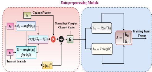
Refer to caption
Figure 3: Dataset Generating Block.

V-B SLP-DNet Training and Testing

The training of DNNs generally involves three steps: forward propagation, backward propagation, and parameter update [42]. Except where necessary, the training SINR is drawn from a random uniform distribution to enable learning over a wide range of SINR values. The PUM contains r blocks, which form a learning layer. Therefore, each block contains three core components and is trained block-wise for l number of iterations.

Similarly, the APB is trained for k iterations. It is important to note that the number of training iterations of the parameter update module may not necessarily be equal to that of the APB. We train the PUM for 15 iterations and the APB for 10 iterations. To improve the training efficiency, we modify the learning rate by a factor α+𝛼superscript\alpha\in\mathbb{R}^{+} for every training step. All the training is done with a stochastic gradient descent algorithm using Adam optimizer [42]. Since the learning is done in an unsupervised fashion, the loss function is the Lagrangian function’s statistical mean over the entire training batch samples. During the inference, a feed-forward pass is performed over the entire architecture using the learned Lagrangian multipliers to calculate the precoding vector using (35) and (62) for both SLP and robust SLP formulations, respectively. Finally, at inference, the trained model is run with different SINR values to obtain the required optimal precoding matrix.

V-C Computational Complexity Evaluation

In this subsection, we analyze and compare the computational costs of the conventional BLP, optimization-based SLP, and the proposed SLP-DNet schemes. The complexities are evaluated in terms of the number of real arithmetic operations involved. For ease of analysis, we convert the SOCP (11) into a standard linear programming (LP)

min{𝐳}𝐳min\displaystyle\underset{\mathbf{\{z\}}}{\text{min}} 𝐜T𝐳superscript𝐜𝑇𝐳\displaystyle\mathbf{c}^{T}\mathbf{z} (63)
s.t. 𝐜kT𝐳tanϕΓiv0,isuperscriptsubscript𝐜𝑘𝑇𝐳tanitalic-ϕsubscriptΓ𝑖subscript𝑣0for-all𝑖\displaystyle\mathbf{c}_{k}^{T}\mathbf{z}\leq{-\text{tan}\phi\sqrt{\Gamma_{i}v_{0}}}\ ,\ \forall{i}

where 𝐜=[𝟎𝐰𝟏𝐓]T(2Nt+1)×1𝐜superscriptmatrix0superscriptsubscript𝐰1𝐓𝑇superscript2subscript𝑁𝑡11\displaystyle\mathbf{c=\begin{bmatrix}0&\mathbf{w}_{1}^{T}\end{bmatrix}}^{T}\in\mathbb{R}^{(2N_{t}+1)\times{1}}, 𝐳=[1𝐰1]T(2Nt+1)×1𝐳superscriptmatrix1subscript𝐰1𝑇superscript2subscript𝑁𝑡11\mathbf{z}=\begin{bmatrix}1&\mathbf{w}_{1}\end{bmatrix}^{T}\in\mathbb{R}^{(2N_{t}+1)\times 1}, 𝐜k=[|𝚲iT𝚷𝐰1|𝚲iTtanϕ]T(2Nt+1)×1subscript𝐜𝑘superscriptdelimited-[]superscriptsubscript𝚲𝑖𝑇𝚷subscript𝐰1superscriptsubscript𝚲𝑖𝑇italic-ϕ𝑇superscript2subscript𝑁𝑡11\mathbf{c}_{k}=\left[\left|\bm{\Lambda}_{i}^{T}\bm{\Pi}\mathbf{w}_{1}\right|\ \bm{\Lambda}_{i}^{T}\tan\phi\right]^{T}\in\mathbb{R}^{(2N_{t}+1)\times 1} and 𝐖=[𝐰11,,𝐰1K];i=1,,Kformulae-sequence𝐖subscript𝐰11subscript𝐰1𝐾for-all𝑖1𝐾\mathbf{W}=[\mathbf{w}_{11},\cdots,\mathbf{w}_{1K}];\ \ \forall{i=1,\cdots,K}. The complexity per iteration for solving convex optimization via IPM is dominated by the formation (𝙲formsubscript𝙲form\mathtt{C}_{\text{form}}) and factorization (𝙲factsubscript𝙲fact\mathtt{C}_{\text{fact}}) of the matrix coefficients of m𝑚m linear equations in m𝑚m unknowns [43]. For generic IPMs, the complexity is expressed as [43]

𝙲total=𝙲iter(𝙲form+𝙲fact)subscript𝙲totalsubscript𝙲itersubscript𝙲formsubscript𝙲fact\mathtt{C}_{\text{total}}=\mathtt{C}_{\text{iter}}\cdot\left(\mathtt{C}_{\text{form}}+\mathtt{C}_{\text{fact}}\right) (64)

where 𝙲itersubscript𝙲iter\mathtt{C}_{\text{iter}} is the iteration complexity required to attain an optimal solution. For a given optimal target accuracy, ϵ>0italic-ϵ0\epsilon>0, 𝙲itersubscript𝙲iter\mathtt{C}_{\text{iter}} is given by

𝙲iter=j=1Nlcdj+2Nsc×ln(1ϵ)subscript𝙲itersuperscriptsubscript𝑗1subscript𝑁lcsubscript𝑑𝑗2subscript𝑁sc1italic-ϵ\mathtt{C}_{\text{iter}}=\sqrt{\sum_{j=1}^{N_{\text{lc}}}{d}_{j}+2N_{\text{sc}}}\times{\ln\left(\frac{1}{\epsilon}\right)} (65)

where d𝑑d is the dimension of the constraints, Nlcsubscript𝑁lcN_{\text{lc}} and Nscsubscript𝑁scN_{\text{sc}} are the numbers of linear inequality matrix and second order cone (SOC) constraints, respectively. The costs of formation and factorization of matrix are respectively given by [43]

𝙲form=mj=1Nlcdj3+m2j=1Nlcdj2due to Nlc+mj=1Nscdj=12due to Nsc;𝙲fact=m3.formulae-sequencesubscript𝙲formsubscript𝑚superscriptsubscript𝑗1subscript𝑁lcsuperscriptsubscript𝑑𝑗3superscript𝑚2superscriptsubscript𝑗1subscript𝑁lcsuperscriptsubscript𝑑𝑗2due to Nlcsubscript𝑚superscriptsubscript𝑗1subscript𝑁scsuperscriptsubscript𝑑𝑗12due to Nscsubscript𝙲factsuperscript𝑚3\mathtt{C}_{\text{form}}=\underbrace{m\sum_{j=1}^{N_{\text{lc}}}d_{j}^{3}+m^{2}\sum_{j=1}^{N_{\text{lc}}}d_{j}^{2}}_{\text{due to $N_{\text{lc}}$}}+\underbrace{m\sum_{j=1}^{N_{\text{sc}}}d_{j=1}^{2}}_{\text{due to $N_{\text{sc}}$}};\ \mathtt{C}_{\text{fact}}=m^{3}. (66)

Specifically, we observe that problem (63) has K𝐾K constraints with dimension 2Nt+12subscript𝑁𝑡12N_{t}+1. Therefore, using (65) and (66), the total computational complexity is thus

𝙲total=2Nt+1[m(2Nt+1)+m(2Nt+1)2+m3]ln(1ϵ)subscript𝙲total2subscript𝑁𝑡1delimited-[]𝑚2subscript𝑁𝑡1𝑚superscript2subscript𝑁𝑡12superscript𝑚31italic-ϵ\mathtt{C}_{\text{total}}=\sqrt{2N_{t}+1}\left[m(2N_{t}+1)+m(2N_{t}+1)^{2}+m^{3}\right]\ln{\left(\frac{1}{\epsilon}\right)}.

(67)

The complexity of BLP can be derived in a similar way and is shown directly in Table I. Conversely, the complexity of the proposed SLP-DNet schemes is the sum of PUM and the APB complexities. Moreover, the complexity of the PUM is dominated by the costs of computing the ‘log barrier’ and the feed-forward pass of the shallow CNN (see Table III) that makes up the barrier term associated with the inequality constraint. Similarly, the complexity of the APB is also obtained by computing the arithmetic operations involved during the forward pass of the deep CNN (see Table IV). To derive the analytical complexity of SLP-DNet, we assume a sliding window is used to perform the dominant computation of the convolution operation in the CNN and ignore the nonlinear computational overhead due to activations. Therefore, the total computational complexity is expressed as

CSLPDNet=Clog-br+2l=1Lconvnh[l1]nw[l1][Cin[l1]f[l]2+1]Cout[l]+j=1Lfc(2Min[j1]+1)Mout[i]subscript𝐶𝑆𝐿𝑃𝐷𝑁𝑒𝑡subscript𝐶log-br2subscriptsuperscriptsubscript𝐿conv𝑙1superscriptsubscript𝑛hdelimited-[]𝑙1superscriptsubscript𝑛wdelimited-[]𝑙1delimited-[]superscriptsubscript𝐶indelimited-[]𝑙1superscript𝑓delimited-[]𝑙21superscriptsubscript𝐶outdelimited-[]𝑙subscriptsuperscriptsubscript𝐿fc𝑗12superscriptsubscript𝑀indelimited-[]𝑗11superscriptsubscript𝑀outdelimited-[]𝑖C_{SLP-DNet}=C_{\text{log-br}}+\\ 2\sum^{L_{\text{conv}}}_{l=1}n_{\text{h}}^{[l-1]}n_{\text{w}}^{[l-1]}\left[C_{\text{in}}^{[l-1]}f^{[l]2}+1\right]C_{\text{out}}^{[l]}+\\ \sum^{L_{\text{fc}}}_{j=1}\left(2M_{\text{in}}^{[j-1]}+1\right)M_{\text{out}}^{[i]} (68)

where nhsubscript𝑛hn_{\text{h}}, nwsubscript𝑛wn_{\text{w}}, f𝑓f, Cinsubscript𝐶inC_{\text{in}} and Coutsubscript𝐶outC_{\text{out}} are the height, width of the input tensor, kernel size, number of input and output channels, respectively. Similarly, Lconvsubscript𝐿convL_{\text{conv}}, Lfcsubscript𝐿fcL_{\text{fc}}, Minsubscript𝑀inM_{\text{in}} and Moutsubscript𝑀outM_{\text{out}} are the number of convolution and fully connected (FC) layers, number of input and output neurons in the FC layer, respectively. Clog-brsubscript𝐶log-brC_{\text{log-br}} denotes the complexity of the ‘log-barrier’ function. Table I shows the summary of the computational complexities of our proposals and the benchmark precoding schemes. As an illustration, we consider the case of a symmetrical system (Nt=K=n)subscript𝑁𝑡𝐾𝑛(N_{t}=K=n), and show that the proposed approach has substantially reduced computational complexity of \mathbcalO(n3)\mathbcal𝑂superscript𝑛3\mathbcal{O}(n^{3}), while the optimization-based SLP approach of \mathbcalO(n6.5)\mathbcal𝑂superscript𝑛6.5\mathbcal{O}(n^{6.5}) and the conventional BLP is \mathbcalO(n7.5)\mathbcal𝑂superscript𝑛7.5\mathbcal{O}(n^{7.5}).

Table I: Complexity analysis of proposed SLP-DNet and benchmark SLP schemes.
Problem Arithmetic Operations (term; m=𝒪(2NtK)𝑚𝒪2subscript𝑁𝑡𝐾m=\mathcal{O}(2N_{t}K)) Complexity Order (n=Nt=K𝑛subscript𝑁𝑡𝐾n=N_{t}=K)
Conventional BLP (4Nt+K+2)[m(2Nt+1)+m(2Nt+1)2+m(K+1)2+m3]ln(1ϵ)4subscript𝑁𝑡𝐾2delimited-[]𝑚2subscript𝑁𝑡1𝑚superscript2subscript𝑁𝑡12𝑚superscript𝐾12superscript𝑚31italic-ϵ\sqrt{(4N_{t}+K+2)}\left[m(2N_{t}+1)+m(2N_{t}+1)^{2}+m(K+1)^{2}+m^{3}\right]\ln{\left(\frac{1}{\epsilon}\right)} 𝒪(n6.5)𝒪superscript𝑛6.5\mathcal{O}(n^{6.5})
SLP Optimization-based 2Nt+1[m(2Nt+1)+m(2Nt+1)2+m3]ln(1ϵ)2subscript𝑁𝑡1delimited-[]𝑚2subscript𝑁𝑡1𝑚superscript2subscript𝑁𝑡12superscript𝑚31italic-ϵ\sqrt{2N_{t}+1}\left[m(2N_{t}+1)+m(2N_{t}+1)^{2}+m^{3}\right]\ln{\left(\frac{1}{\epsilon}\right)} 𝒪(n6.5)𝒪superscript𝑛6.5\mathcal{O}(n^{6.5})
SLP-DNet 4K2Nt+42K2+48KNt+512K+24superscript𝐾2subscript𝑁𝑡42superscript𝐾248𝐾subscript𝑁𝑡512𝐾24K^{2}N_{t}+42K^{2}+48KN_{t}+512K+2 𝒪(n3)𝒪superscript𝑛3\mathcal{O}(n^{3})
SLP-DNet Strict 4K2Nt+39K2+46KNt+512K+24superscript𝐾2subscript𝑁𝑡39superscript𝐾246𝐾subscript𝑁𝑡512𝐾24K^{2}N_{t}+39K^{2}+46KN_{t}+512K+2 𝒪(n3)𝒪superscript𝑛3\mathcal{O}(n^{3})
Robust Conventional BLP 2K(2Nt+1)[mK(2Nt+1)3+m2K(2Nt+1)2+m3]ln(1ϵ)2𝐾2subscript𝑁𝑡1delimited-[]𝑚𝐾superscript2subscript𝑁𝑡13superscript𝑚2𝐾superscript2subscript𝑁𝑡12superscript𝑚31italic-ϵ\sqrt{2K(2N_{t}+1)}\left[mK(2N_{t}+1)^{3}+m^{2}K(2N_{t}+1)^{2}+m^{3}\right]\ln{\left(\frac{1}{\epsilon}\right)} 𝒪(n7.5)𝒪superscript𝑛7.5\mathcal{O}(n^{7.5})
Robust SLP Optimization-based 2(2Nt+1)[2mK(2Nt+1)2+m3]ln(1ϵ)22subscript𝑁𝑡1delimited-[]2𝑚𝐾superscript2subscript𝑁𝑡12superscript𝑚31italic-ϵ\sqrt{2(2N_{t}+1)}\left[2mK(2N_{t}+1)^{2}+m^{3}\right]\ln{\left(\frac{1}{\epsilon}\right)} 𝒪(n6.5)𝒪superscript𝑛6.5\mathcal{O}(n^{6.5})
Robust SLP-DNet 16KNt2+42K2+48KNt+512K16𝐾superscriptsubscript𝑁𝑡242superscript𝐾248𝐾subscript𝑁𝑡512𝐾16KN_{t}^{2}+42K^{2}+48KN_{t}+512K 𝒪(n3)𝒪superscript𝑛3\mathcal{O}(n^{3})

VI Simulation, Results and Discussion

VI-A Simulation Set-up

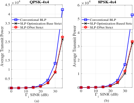
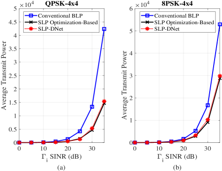
We consider a single-cell MISO downlink in which the BS is equipped with four antennas (Nt=4subscript𝑁𝑡4N_{t}=4) that serve K=4𝐾4K=4 single users. We generate 50,000 training and 2000 test samples of Rayleigh fading channel coefficients, respectively drawn from the same statistical distribution. The transmit data symbols are modulated using QPSK and 8PSK modulation schemes. The training SINR is randomly drawn from uniform distribution Γtrain𝒰(Γlow,Γhigh)similar-tosubscriptΓtrain𝒰subscriptΓlowsubscriptΓhigh\Gamma_{\text{train}}\sim\mathcal{U}(\Gamma_{\text{low}},\,\Gamma_{\text{high}}). Adam optimizer [42] is used for stochastic gradient descent algorithm with Lagrangian function as a loss metric.

Furthermore, a parametric rectified linear unit (PReLu) activation function is used for both convolutional and fully connected layers instead of the traditional ReLu function. The reason for this is to address the problem of dying gradient [42]. The learning rate is reduced by a factor α=0.65𝛼0.65\alpha=0.65 after every iteration to aid the learning algorithm to converge faster. The learning models are implemented in Pytorch 1.7.1 and Python 3.7.8 on a computer with the following specifications: Intel(R) Core (TM) i7-6700 CPU Core, 32.0GB of RAM. Table II summarizes the simulation parameters, while Tables III and IV depict the NN component settings of the SLP-DNet.

Table II: Simulation settings
Parameters Values
Training Samples 50000
Batch Size (B) 200
Test Samples 2000
Training SINR range 0.0dB - 45.0dB
Test SINR range (i-th user SINR) 0.0dB - 35.0dB
Optimizer SGD with Adam
Initial Learning Rate η𝜂\eta 0.001
Learning Rate decay factor α𝛼\alpha 0.65
Weight Initializer Xavier Initializer
Number of blocks in the parameter
update unit Br=2subscript𝐵𝑟2B_{r}=2
Training Iterations for each block
of the parameter update unit 15
Training iterations for the auxiliary unit 10
Table III: Proximity Barrier Function NN Layout
Layer Parameter, kernel size=3×3kernel size33\text{kernel size}=3\times 3
Input Layer Input size (B, 1, 2Nt,K)B12subscript𝑁𝑡𝐾(\text{B},\ 1,\ 2N_{t},\ K)
Layer 1: Convolutional Size (B,1,K,20)B1𝐾20(\text{B},1,K,20); zero padding
Layer 2: Average Pooling Size ((1, 1),stride=(1, 1))11stride11((1,\ 1),\ \text{stride}=(1,\ 1))
Layer 3: Activation Soft-Plus
Layer 4: Flat Size (B×20×K2)B20superscript𝐾2(\text{B}\times 20\times K^{2})
Layer : Fully-connected Size(B×20×K2, 1)B20superscript𝐾21(\text{B}\times 20\times K^{2},\ 1)
Layer 5: Activation Soft-Plus function
Table IV: Auxiliary Processing Block (APB) NN Structure
Layer Parameter, kernel size=3×3kernel size33\text{kernel size}=3\times 3
Input Layer Input size (B, 1, 2Nt,K)B12subscript𝑁𝑡𝐾(\text{B},\ 1,\ 2N_{t},\ K)
Layer 1: Convolutional Size (B, 1,K, 64)B1𝐾64(\text{B},\ 1,\ K,\ 64),
dilation=1dilation1\text{dilation}=1 and unit padding
Layer 2: Batch Normalization eps=106epssuperscript106\text{eps}=10^{-6}, momentum=0.1momentum0.1\text{momentum}=0.1
Layer 3: Activation PReLu
Layer 4: Convolutional Size (B, 1, 64, 2NtK)B1642subscript𝑁𝑡𝐾(\text{B},\ 1,\ 64,\ 2N_{t}K),
dilation=1dilation1\text{dilation}=1 and unit padding
Layer 5: Batch Normalization eps=106epssuperscript106\text{eps}=10^{-6}, momentum=0.1momentum0.1\text{momentum}=0.1
Layer 6: Activation PReLu
Layer 7: Convolutional Size (B, 1, 2NtK, 1)B12subscript𝑁𝑡𝐾1(\text{B},\ 1,\ 2N_{t}K,\ 1),
dilation=1dilation1\text{dilation}=1 and unit padding

VI-B Performance Evaluation of Non-Robust SLP-DNet

In this subsection, we evaluate the performance of our proposed unsupervised learning framework for nonrobust scenario against the benchmark algorithms [30, 2, 40] for both strict and relaxed angle rotations.

Firstly, we compare the average transmit power of the conventional BLP (2), the SLP optimization-based problems (3), (11) and the SLP-DNet precoding scheme based on (28) and Algorithm 2. The performances of SLP-DNet and the benchmark schemes (conventional BLP and SLP optimization-based) for strict angle rotation are shown in Fig. 4. It can be observed that the transmit power of the proposed SLP-DNet closely matches the optimisation based SLP, both with significant gains against BLP.

Similarly, we discern the same trend in Fig. 5 for the relaxed angle scenario as observed in Fig. 4. Accordingly, we find from Fig. 5 that the relaxed angle formulation offers significant power savings over the strict angle formulation and is therefore adopted in the subsequent experiments. Furthermore, at 30dB, the performance of SLP-DNet is within 5% of the SLP optimization-based solution. Thus, while the SLP optimization-based offers a slightly lower transmit power at SINR above 30dB, the proposed learning-based model’s performance is within 96%98%percent96percent9896\%-98\% of the optimization-based solution.

Refer to caption
Figure 4: Transmit Power vs SINR averaged over 2000 test samples for conventional BLP, SLP optimization-based and nonrobust SLP-DNet schemes for 𝕄𝕄\mathbb{M}-PSK modulation with Nt=4subscript𝑁𝑡4N_{t}=4, K=4𝐾4K=4 under strict angle rotation.
Refer to caption
Figure 5: Transmit Power vs SINR averaged over 2000 test samples for conventional BLP, SLP optimization-based and nonrobust SLP-DNet schemes for 𝕄𝕄\mathbb{M}-PSK modulation with Nt=4subscript𝑁𝑡4N_{t}=4, K=4𝐾4K=4 under relaxed angle rotation.

VI-C Performance Evaluation of Robust SLP-DNet

In this subsection, we evaluate the performance of the robust SLP-DNet against the robust SLP optimization-based and conventional precoding algorithms.

Figs. 6 and 7 compare the performance of the proposed robust SLP-DNet with the traditional robust block-level precoder [40] and robust SLP precoder [2] for the 4×4444\times 4 MISO system evaluated at ς2=104superscript𝜍2superscript104\varsigma^{2}={10}^{-4}. For simplicity, we use QPSK modulation scheme. Fig. 6 depicts how the average transmit power increases with the SINR thresholds, for CSI error bounds ς2=104superscript𝜍2superscript104\varsigma^{2}={10}^{-4}. The SLP optimization-based precoding scheme is observed to show a significant power savings of more than 60% compared to the conventional optimization solution. Similarly, the proposed unsupervised learning-based precoder portrays a similar transmit power reduction trend. They show considerable power savings of 40%58%percent40percent5840\%-58\% against the conventional BLP.

Furthermore, we investigate the effect of the CSI error bounds on the transmit power at 30dB. Fig. 7 depicts the transmit power variation with increasing CSI error bounds. Moreover, a significant increase in transmit power can be observed where the channel uncertainty lies within the region of CSI error bounds of ς2=103superscript𝜍2superscript103\varsigma^{2}=10^{-3}. Interestingly, like the SLP optimization-based algorithm, the proposed SLP-DNet also shows a descent or moderate increase in transmit power by exploiting the constructive interference.
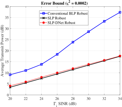
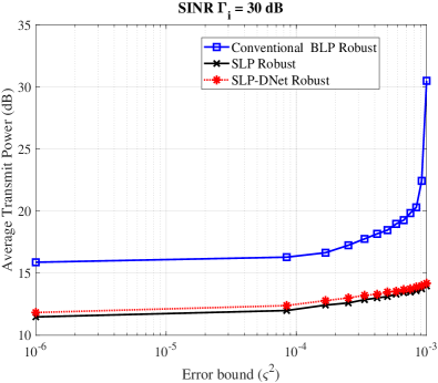
Refer to caption
Figure 6: Transmit Power vs SINR averaged over 2000 test samples for robust conventional, SLP optimization-based and SLP-DNet solutions with Nt=4subscript𝑁𝑡4N_{t}=4, K=4𝐾4K=4 and ς2=0.0002superscript𝜍20.0002\varsigma^{2}=0.0002.
Refer to caption
Figure 7: Transmit Power vs Error-bound for robust conventional BLP, SLP optimization-based and SLP-DNet solutions with Nt=4subscript𝑁𝑡4N_{t}=4, K=4𝐾4K=4.

Figs. 8(a) and 8(b) depict the execution times for nonrobust and robust formulations. It can be seen that both SLP optimization-based algorithm and the proposed learning schemes are feasible for all sets of Ntsubscript𝑁𝑡N_{t} BS antenna and K𝐾K mobile users. However, for conventional BLP, the solution is only feasible for NtKsubscript𝑁𝑡𝐾N_{t}\geq K.

Fig. 8(a) shows the average execution time of the proposed unsupervised learning solutions per symbol averaged over 2000 test samples for nonrobust formulations. The SLP-DNet is observed to be significantly faster than the SLP optimization-based. For example, the theoretical complexity is polynomial order-3 and polynomial order-6.5 or order-7.5 for SLP-DNet and conventional methods, respectively. This is shown in the execution times, where there is a significantly steeper increase in run-time as the number of users increases. The decrease in computational cost is because the dominant operations involved in SLP-DNet at the inference are simple matrix-matrix or vector-matrix convolution. The same trend is also observed in the case of a robust channel scenario, as shown in Fig. 8(b). Therefore, the results in Figs. 8(a) and 8(b) demonstrate that the proposed unsupervised learning-based precoding solutions offer a good trade-off between the performance and computational complexity. Moreover, as per the results obtained, SLP-DNet’s performance is within the range of 89%99%percent89percent9989\%-99\% of the optimal SLP optimization-based precoding solution. Thus, our proposals demonstrate a favorable tradeoff between the performance and the computational complexity involved.
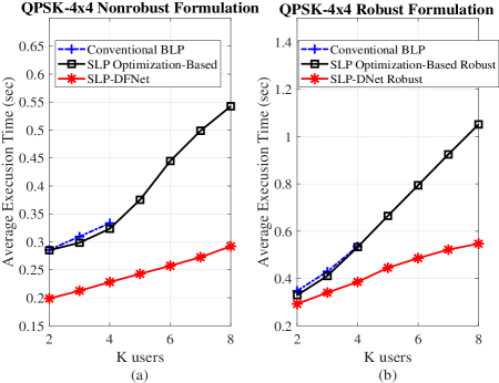
Refer to caption
Figure 8: Comparison of average execution time per sample averaged over 200 test samples for conventional BLP, optimization-based and SLP-DNet solutions with Nt=4subscript𝑁𝑡4N_{t}=4 and K𝐾K users (2,,8)28(2,\cdots,8).

VII Conclusion

This paper proposes an unsupervised learning-based precoding framework for a multi-user downlink MISO system. The proposed learning technique exploits the constructive interference for the power minimization problem so that for given QoS constraints, the transmit power available for transmission is minimized. We use domain knowledge to design unsupervised learning architectures by unfolding the proximal interior point method barrier ‘log’ function. The proposed learning scheme is then extended to robust precoding designs with imperfect CSI bounded by CSI errors. We demonstrate that our proposal is computationally efficient and allows for feasible solutions to be obtained for problems where traditional numerical optimization like IPM and brute-force maximum likelihood solvers would not converge or would be prohibitively costly.

Appendix A Proximity operator barrier for Robust SLP

For every transmit precoding vector 𝐰22Nt×1subscript𝐰2superscript2subscript𝑁𝑡1\mathbf{w}_{2}\in\mathbb{R}^{2N_{t}\times 1}, the proximity operator of the barrier γμBrobust(𝐰2)𝛾𝜇subscript𝐵robustsubscript𝐰2\gamma\mu{B}_{\text{robust}}(\mathbf{w}_{2}) is given by

Φrb(𝐰2,γ,μ)=2Γv0tan2ϕX(𝐰2,γ,μ)22Γv0tan2ϕX(𝐰2,γ,μ)2+2γμ𝐰2subscriptΦrbsubscript𝐰2𝛾𝜇2Γsubscript𝑣0superscripttan2italic-ϕ𝑋superscriptsubscript𝐰2𝛾𝜇22Γsubscript𝑣0superscripttan2italic-ϕ𝑋superscriptsubscript𝐰2𝛾𝜇22𝛾𝜇subscript𝐰2\Phi_{\text{rb}}(\mathbf{w}_{2},\gamma,\mu)=\frac{2\Gamma{v}_{0}\text{tan}^{2}{\phi}-X(\mathbf{w}_{2},\gamma,\mu)^{2}}{2\Gamma{v}_{0}\text{tan}^{2}{\phi}-X(\mathbf{w}_{2},\gamma,\mu)^{2}+2\gamma\mu}{\mathbf{w}_{2}} (69)

where X(𝐰2,γ,μ)𝑋subscript𝐰2𝛾𝜇X(\mathbf{w}_{2},\gamma,\mu) is the unique solution of the cubic equation expressed as [33]

x3((ς2𝚲T𝚲)𝐰22+4𝚲T𝐰2tanϕΓv0)x2+(2Γv0tan2ϕ+2γμ)x+2Γv0tan2ϕ((ς2𝚲T𝚲)𝐰22+4𝚲T𝐰2tanϕΓv0)=0.superscript𝑥3superscript𝜍2superscript𝚲𝑇𝚲subscriptdelimited-∥∥subscript𝐰224superscript𝚲𝑇subscript𝐰2tanitalic-ϕΓsubscript𝑣0superscript𝑥2missing-subexpressionlimit-from2Γsubscript𝑣0superscripttan2italic-ϕ2𝛾𝜇𝑥missing-subexpression2Γsubscript𝑣0superscripttan2italic-ϕsuperscript𝜍2superscript𝚲𝑇𝚲subscriptdelimited-∥∥subscript𝐰224superscript𝚲𝑇subscript𝐰2tanitalic-ϕΓsubscript𝑣00missing-subexpression\leavevmode\resizebox{446.2658pt}{}{$\begin{array}[]{ll}{x}^{3}-\left(\left(\varsigma^{2}-\bm{\Lambda}^{T}\bm{\Lambda}\right)\left\lVert\mathbf{w}_{2}\right\rVert_{2}+4\bm{\Lambda}^{T}\mathbf{w}_{2}\text{tan}{\phi}\sqrt{\Gamma{v}_{0}}\right){x}^{2}\\ +\left(2\Gamma{v}_{0}\text{tan}^{2}{\phi}+2\gamma\mu\right){{x}}+\\ 2\Gamma{v}_{0}\text{tan}^{2}{\phi}\left(\left(\varsigma^{2}-\bm{\Lambda}^{T}\bm{\Lambda}\right)\left\lVert\mathbf{w}_{2}\right\rVert_{2}+4\bm{\Lambda}^{T}\mathbf{w}_{2}\text{tan}{\phi}\sqrt{\Gamma{v}_{0}}\right)=0.\end{array}$} (70)

It can be observed that (70) is a cubic equation and can be solved analytically. In the final analysis, following similar steps as in (22)-(26), the robust deep-unfolded model is obtained by finding the Jacobean matrix of (69) with respect to the optimization variable 𝐰2subscript𝐰2\mathbf{w}_{2}, and the derivatives with respect to the step-size γ>0𝛾0\gamma>0 and the Lagrange multiplier associated with the inequality constraint μ>0𝜇0\mu>0. We use similar concepts presented in subsection III-B to formulate the learning algorithm of the robust SLP as a series of sub-problems with respect to the combined effect of the two inequality constraints as follows

min𝐰𝟐𝟐𝐍𝐭×𝟏subscript𝐰2superscript2subscript𝐍𝐭1min\displaystyle\underset{\mathbf{w_{2}\in{\mathbb{R}}^{2N_{t}\times 1}}}{\text{min}} 𝐰222+λ𝐰2+μBrobust(𝐰2).superscriptsubscriptdelimited-∥∥subscript𝐰222𝜆subscript𝐰2𝜇subscript𝐵robustsubscript𝐰2\displaystyle{\left\lVert\mathbf{w}_{2}\right\rVert}_{2}^{2}+\lambda{\mathbf{w}_{2}}+{\mu}{{B}_{\text{robust}}(\mathbf{w}_{2})}. (71)

Similar to a nonrobust SLP-DNet, the update rule for every iteration is expressed as

𝐰2[r+1]=proxγ[r]μ[r]Brobust(𝐰2[r]γ[r]ΔDrobust(𝐰2[r],λ[r]))superscriptsubscript𝐰2delimited-[]𝑟1subscriptproxsuperscript𝛾delimited-[]𝑟superscript𝜇delimited-[]𝑟subscript𝐵robustsuperscriptsubscript𝐰2delimited-[]𝑟superscript𝛾delimited-[]𝑟Δsubscript𝐷robustsuperscriptsubscript𝐰2delimited-[]𝑟superscript𝜆delimited-[]𝑟\mathbf{w}_{2}^{[r+1]}=\text{prox}_{\gamma^{[r]}{\mu}^{[r]}B_{\text{robust}}}\left(\mathbf{w}_{2}^{[r]}-\gamma^{[r]}\Delta{{D}_{\text{robust}}(\mathbf{w}_{2}^{[r]},\lambda^{[r]})}\right) (72)

where

Drobust(𝐰2[r],λ[r])=𝐰222+λ𝐰2.subscript𝐷robustsuperscriptsubscript𝐰2delimited-[]𝑟superscript𝜆delimited-[]𝑟superscriptsubscriptdelimited-∥∥subscript𝐰222𝜆subscript𝐰2{D}_{\text{robust}}(\mathbf{w}_{2}^{[r]},\lambda^{[r]})={\left\lVert\mathbf{w}_{2}\right\rVert}_{2}^{2}+\lambda{\mathbf{w}_{2}}. (73)

References

  • [1] C. Masouros and T. Ratnarajah, “Interference as a source of green signal power in cognitive relay assisted co-existing mimo wireless transmissions,” IEEE Transactions on Communications, vol. 60, no. 2, pp. 525–536, 2011.
  • [2] C. Masouros and G. Zheng, “Exploiting known interference as green signal power for downlink beamforming optimization,” IEEE Transactions on Signal processing, vol. 63, no. 14, pp. 3628–3640, 2015.
  • [3] C. Masouros, “Harvesting signal power from constructive interference in multiuser downlinks,” in Wireless Information and Power Transfer: A New Paradigm for Green Communications.   Springer, 2018, pp. 87–122.
  • [4] Y. Ni, S. Jin, W. Xu, Y. Wang, M. Matthaiou, and H. Zhu, “Beamforming and interference cancellation for d2d communication underlaying cellular networks,” IEEE Transactions on Communications, vol. 64, no. 2, pp. 832–846, 2015.
  • [5] S. Hong, J. Brand, J. I. Choi, M. Jain, J. Mehlman, S. Katti, and P. Levis, “Applications of self-interference cancellation in 5g and beyond,” IEEE Communications Magazine, vol. 52, no. 2, pp. 114–121, 2014.
  • [6] C. Masouros and E. Alsusa, “A novel transmitter-based selective-precoding technique for ds/cdma systems,” in 2007 IEEE International Conference on Communications.   IEEE, 2007, pp. 2829–2834.
  • [7] C. Masouros and E. Alsusa, “Dynamic linear precoding for the exploitation of known interference in mimo broadcast systems,” IEEE Transactions on Wireless Communications, vol. 8, no. 3, pp. 1396–1404, 2009.
  • [8] C. Masouros, “Correlation rotation linear precoding for mimo broadcast communications,” IEEE Transactions on Signal Processing, vol. 59, no. 1, pp. 252–262, 2010.
  • [9] C. Masouros, M. Sellathurai, and T. Ratnarajah, “Vector perturbation based on symbol scaling for limited feedback miso downlinks,” IEEE Transactions on Signal Processing, vol. 62, no. 3, pp. 562–571, 2014.
  • [10] M. Alodeh, S. Chatzinotas, and B. Ottersten, “Constructive multiuser interference in symbol level precoding for the miso downlink channel,” IEEE Transactions on Signal processing, vol. 63, no. 9, pp. 2239–2252, 2015.
  • [11] P. V. Amadori and C. Masouros, “Constant envelope precoding by interference exploitation in phase shift keying-modulated multiuser transmission,” IEEE Transactions on Wireless Communications, vol. 16, no. 1, pp. 538–550, 2016.
  • [12] M. Alodeh, S. Chatzinotas, and B. Ottersten, “Symbol-level multiuser miso precoding for multi-level adaptive modulation,” IEEE Transactions on Wireless Communications, vol. 16, no. 8, pp. 5511–5524, 2017.
  • [13] A. Li, C. Masouros, F. Liu, and A. L. Swindlehurst, “Massive mimo 1-bit dac transmission: A low-complexity symbol scaling approach,” IEEE Transactions on Wireless Communications, vol. 17, no. 11, pp. 7559–7575, 2018.
  • [14] A. Li and C. Masouros, “A two-stage vector perturbation scheme for adaptive modulation in downlink mu-mimo,” IEEE Transactions on Vehicular Technology, vol. 65, no. 9, pp. 7785–7791, 2015.
  • [15] S. Timotheou, G. Zheng, C. Masouros, and I. Krikidis, “Exploiting constructive interference for simultaneous wireless information and power transfer in multiuser downlink systems,” IEEE Journal on Selected Areas in Communications, vol. 34, no. 5, pp. 1772–1784, 2016.
  • [16] A. Li and C. Masouros, “Exploiting constructive mutual coupling in p2p mimo by analog-digital phase alignment,” IEEE Transactions on Wireless Communications, vol. 16, no. 3, pp. 1948–1962, 2017.
  • [17] D. Spano, M. Alodeh, S. Chatzinotas, and B. Ottersten, “Symbol-level precoding for the nonlinear multiuser miso downlink channel,” IEEE Transactions on Signal Processing, vol. 66, no. 5, pp. 1331–1345, 2017.
  • [18] A. Kalantari, C. Tsinos, M. Soltanalian, S. Chatzinotas, W.-K. Ma, and B. Ottersten, “Spatial peak power minimization for relaxed phase m-psk mimo directional modulation transmitter,” in 2017 25th European Signal Processing Conference (EUSIPCO).   IEEE, 2017, pp. 2011–2015.
  • [19] K. L. Law, C. Masouros, and M. Pesavento, “Transmit precoding for interference exploitation in the underlay cognitive radio z-channel,” IEEE Transactions on Signal Processing, vol. 65, no. 14, pp. 3617–3631, 2017.
  • [20] A. Li and C. Masouros, “Interference exploitation precoding made practical: Optimal closed-form solutions for psk modulations,” IEEE Transactions on Wireless Communications, vol. 17, no. 11, pp. 7661–7676, 2018.
  • [21] A. Mohammad, C. Masouros, and Y. Andreopoulos, “Complexity-scalable neural-network-based mimo detection with learnable weight scaling,” IEEE Transactions on Communications, vol. 68, no. 10, pp. 6101–6113, 2020.
  • [22] A. Alkhateeb, S. Alex, P. Varkey, Y. Li, Q. Qu, and D. Tujkovic, “Deep learning coordinated beamforming for highly-mobile millimeter wave systems,” IEEE Access, vol. 6, pp. 37 328–37 348, 2018.
  • [23] A. Mohammad, C. Masouros, and Y. Andreopoulos, “Accelerated learning-based mimo detection through weighted neural network design,” in ICC 2020-2020 IEEE International Conference on Communications (ICC).   IEEE, 2020, pp. 1–6.
  • [24] H. Huang, W. Xia, J. Xiong, J. Yang, G. Zheng, and X. Zhu, “Unsupervised learning-based fast beamforming design for downlink mimo,” IEEE Access, vol. 7, pp. 7599–7605, 2018.
  • [25] H. Sun, X. Chen, Q. Shi, M. Hong, X. Fu, and N. D. Sidiropoulos, “Learning to optimize: Training deep neural networks for interference management,” IEEE Transactions on Signal Processing, vol. 66, no. 20, pp. 5438–5453, 2018.
  • [26] W. Xia, G. Zheng, Y. Zhu, J. Zhang, J. Wang, and A. P. Petropulu, “A deep learning framework for optimization of miso downlink beamforming,” IEEE Transactions on Communications, vol. 68, no. 3, pp. 1866–1880, 2019.
  • [27] H. Huang, Y. Peng, J. Yang, W. Xia, and G. Gui, “Fast beamforming design via deep learning,” IEEE Transactions on Vehicular Technology, vol. 69, no. 1, pp. 1065–1069, 2019.
  • [28] Z. Lei, X. Liao, Z. Gao, and A. Li, “Ci-nn: A model-driven deep learning based constructive interference precoding scheme,” IEEE Communications Letters, 2021.
  • [29] P. de Kerret and D. Gesbert, “Robust decentralized joint precoding using team deep neural network,” in 2018 15th International Symposium on Wireless Communication Systems (ISWCS).   IEEE, 2018, pp. 1–5.
  • [30] E. Björnson, M. Bengtsson, and B. Ottersten, “Optimal multiuser transmit beamforming: A difficult problem with a simple solution structure [lecture notes],” IEEE Signal Processing Magazine, vol. 31, no. 4, pp. 142–148, 2014.
  • [31] C. Masouros, T. Ratnarajah, M. Sellathurai, C. Papadias, and A. Shukla, “Known interference in wireless communications: a limiting factor or a potential source of green signal power?” IEEE Comms. Mag, vol. 51, no. 10, pp. 162–171, 2013.
  • [32] A. Li, D. Spano, J. Krivochiza, S. Domouchtsidis, C. G. Tsinos, C. Masouros, S. Chatzinotas, Y. Li, B. Vucetic, and B. Ottersten, “A tutorial on interference exploitation via symbol-level precoding: Overview, state-of-the-art and future directions,” IEEE Communications Surveys & Tutorials, vol. 22, no. 2, pp. 796–839, 2020.
  • [33] C. Bertocchi, E. Chouzenoux, M.-C. Corbineau, J.-C. Pesquet, and M. Prato, “Deep unfolding of a proximal interior point method for image restoration,” Inverse Problems, vol. 36, no. 3, p. 034005, 2020.
  • [34] R. Hauser, “Interior-point methods for inequality constrained optimization,” 2007.
  • [35] N. Pustelnik and L. Condat, “Proximity operator of a sum of functions; application to depth map estimation,” IEEE Signal Processing Letters, vol. 24, no. 12, pp. 1827–1831, 2017.
  • [36] S. Boyd, S. P. Boyd, and L. Vandenberghe, Convex optimization.   Cambridge university press, 2004.
  • [37] S. Ioffe and C. Szegedy, “Batch normalization: Accelerating deep network training by reducing internal covariate shift,” in International conference on machine learning.   PMLR, 2015, pp. 448–456.
  • [38] H. Zheng, Z. Yang, W. Liu, J. Liang, and Y. Li, “Improving deep neural networks using softplus units,” in 2015 International Joint Conference on Neural Networks (IJCNN).   IEEE, 2015, pp. 1–4.
  • [39] B. Wang and D. Klabjan, “Regularization for unsupervised deep neural nets,” in Proceedings of the Thirty-First AAAI Conference on Artificial Intelligence, 2017, pp. 2681–2681.
  • [40] G. Zheng, K.-K. Wong, and T.-S. Ng, “Robust linear mimo in the downlink: A worst-case optimization with ellipsoidal uncertainty regions,” EURASIP Journal on Advances in Signal Processing, vol. 2008, pp. 1–15, 2008.
  • [41] N. Parikh and S. Boyd, “Proximal algorithms,” Foundations and Trends in optimization, vol. 1, no. 3, pp. 127–239, 2014.
  • [42] S. Shalev-Shwartz and S. Ben-David, Understanding machine learning: From theory to algorithms.   Cambridge university press, 2014.
  • [43] K.-Y. Wang, A. M.-C. So, T.-H. Chang, W.-K. Ma, and C.-Y. Chi, “Outage constrained robust transmit optimization for multiuser miso downlinks: Tractable approximations by conic optimization,” IEEE Transactions on Signal Processing, vol. 62, no. 21, pp. 5690–5705, 2014.