A Family of Multi-Asset Automated Market Makers
Abstract
We present a family of multi-asset automated market makers whose liquidity curves are derived from the financial principles of self financing transactions and rebalancing. The constant product market maker emerges as a special case.
1 Introduction
To fix notation, we consider asset tokens in a pool with denoting the price of token at time and denoting the number of token in the pool at time so that
is the value of token at time . In addition, we require the existence of a token specific to each pool that acts both as a liability and a numeraire to the other asset tokens so that all asset tokens are priced in terms of the pool token. We assign the index to the pool token so that the total value of the pool is given by
where we used the fact that since the pool token is the numeraire, its price (in terms of itself) is always . Furthermore, we require the total value of the pool to be zero so that the pool token is a liability with value given by
From this point, the derivation of the new liquidity curves follows from assuming:
-
•
All transactions are self financing.
-
•
The pool has a specified rebalancing strategy.
2 Self Financing
For any variable relating to token at time , let
denote its change from time to time and let
denote a weighted average of the value between time and time with weight . A discrete product rule can be written as
The right-hand side of the above is independent of the choice of , which merely specifies different decompositions of the product rule.
With this discrete product rule, the change in value of a token in the pool can then be expressed as
This can be decomposed into a change of value due to trading activity
and a change in value due to price movements
A pool of tokens is self financing if the total change in value due to trading activity is zero, i.e.
so that
| (1) |
It follows that the total value due to market movement is also zero because we assumed the total value of the pool is always zero, i.e.
so that
where the sum starts at because for all so that
3 Rebalancing Strategies
The final ingredient needed to derive the liquidity curve is to require a specified rebalancing strategy for the pool. The weight of an asset token in the pool at time is the ratio of its value to the total value of all asset tokens in the pool, i.e.
for ranging over asset tokens to so that
A rebalancing strategy is a specification of all weights at time given information no later than time . For a given rebalancing strategy, the price of a token at time is given by
| (2) |
4 Liquidity Curves
A liquidity curve is the foundation of an automated market maker (AMM) and represents a constraint among token number growths (and hence price changes) in an -asset pool
where
is the token number growth factor for token from time to .
To derive the liquidity curves, we simply combine the self financing formula (1) with the price formula (2) from the rebalancing strategy, i.e.
The above can be rewritten as a one-parameter family of liquidity curves given by
| (3) |
If we assume equal weights so that , then we have the liquidity curves
| (4) |
5 Asset Swaps
Consider an equally-weighted pool with asset tokens and we wish to swap the first two. It follows that and the liquidity curve becomes
| (5) |
which is notably independent of When , the liquidity curve simplifies further to
which is equivalent to the familiar constant product market maker
| (6) |
as originally used by Uniswap [1] for and Balancer [2] for .
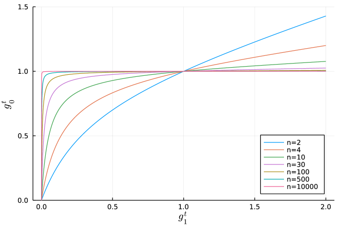
Liquidity curves for various values of are illustrated in Figure 1.
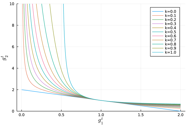
All curves are bounded below by with liquidity curve
| (7) |
and above by with liquidity curve
| (8) |
with the constant product curve in between.
The lowest liquidity curve corresponding to does not produce a practical market maker since the constraint is linear even when all of one token is swapped out of the pool. However, for all we get the desired nonlinearities and letting approach 0 shifts the nonlinearity closer to as illustrated in Figure 2.
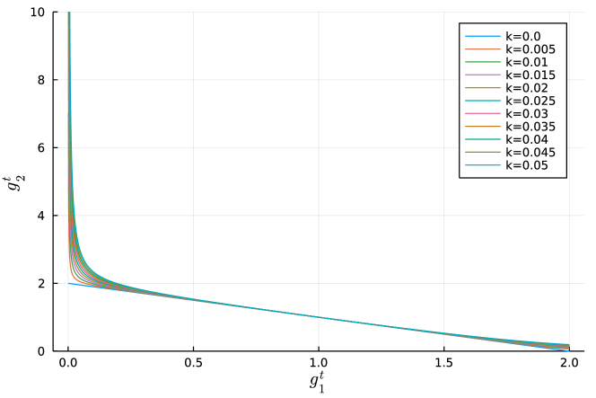
These liquidity curves near are most appropriate for swaps between liquid stablecoins referencing the same fiat currency.
At the other extreme, when there is a discontinuity at since
| (9) |
This discontinuity represents a valid market maker, but with a restriction that no more than half the asset tokens in a pool can be swapped out in a single transaction. The liquidity curve for is a special case and for any other , the liquidity curves all spike as approaches zero, i.e. as all of asset token 1 is removed from the pool in a single transaction. Liquidity curves near are illustrated in Figure 3.
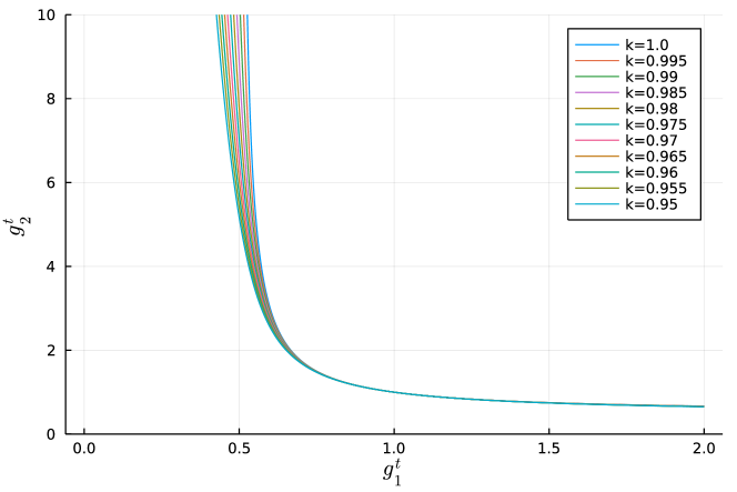
These market makers maximize the price impact of all trades and would be especially suitable for illiquid asset tokens, but remain suitable for any asset token especially when each transaction is small relative to the total size of the pool.
The constant product market maker corresponding to is a special case of the general one-parameter family of automated market makers.
6 Staking
Staking is simply a swap that involves receiving pool tokens in exchange for one or more asset tokens. There are no pool tokens in the pool per se so when asset tokens are staked, pool tokens are minted. Conversely, when asset tokens are unstaked, pool tokens are burned.
When asset tokens are staked in the same proportion, i.e. , the liquidity curve collapses trivially to
and the pool token grows in the same proportion. When and this corresponds to Uniswap and its cousins. However, when a single asset token is staked, the liquidity curve may be written as
| (10) |
and the number of pool tokens minted depends on both the number of asset tokens in the pool and the value of . Figure 4 illustrates the one-asset staking curve as a function of for a 10-asset pool.
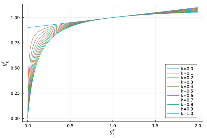
Similarly, Figure 5 illustrates the one-asset staking curve as a function of the number of asset tokens for
The case of and in Figure 5 illustrates what a version of Uniswap would look like if it allowed one-sided staking. As the number of asset tokens in the pool increases, shared liquidity among asset tokens naturally mutes the price impact, i.e. flattens the liquidity curve, when staking and unstaking.
7 Multi-Token Swaps
In the preceding analysis, we considered multi-token swaps when all asset tokens are swapped in the same proportion and we considered simple swaps between any two tokens, where a two-token swap involving the pool token represents one-sided staking. However, the proposed model facilitates more general multi-token swaps involving any number of tokens in any proportions. The equally-weighted -asset liquidity curve (4) contains degrees of freedom in the form of the token number growth factors . If we specify any growth factors, we can use the liquidity curve to solve for the remaining growth factor.
For example, if we wish to swap the first asset tokens in an -asset pool so that for and the liquidity curve becomes
| (11) |
which is a generalization of (5) and, again, is notably independent of To settle this multi-asset swap, we would need to first specify the growth factors for of the assets and use the liquidity curve (11) to solve for the remaining growth factor.
As a special case when , the general equally-weighted -asset liquidity curve (4) simplifies to
i.e. the growth in pool tokens is the average growth of the asset tokens for a single transaction. If you wished to stake any number of asset tokens in any proportion, the liquidity curve tells you how many pool tokens you would receive. Similarly, when , the liquidity curve becomes
and when which is related to Uniswap for and Balancer for , we have
In particular, when and , we have
which is valid for any arbitrary multi-asset swap, but swapping any two asset tokens and in the pool (like Uniswap / Balancer) results in
as highlighted in (6) above.
8 Conclusions and Future Work
We presented a one-parameter family of liquidity curves in (3) derived from simple financial principles assuming all trades are self financing and that the pool imposes a rebalancing strategy. These liquidity curves then form the basis for a new one-parameter family of AMMs.
When the asset token weights are equal, we saw that the liquidity curves were independent of the number of asset tokens in the pool for pure asset token swaps, but the shared liquidity among asset tokens reduces the price impact for swaps that involve the pool token when staking and unstaking.
We saw that liquidity curves near were largely insensitive to the size of the swap and are most suitable for swapping stablecoins referencing the same fiat currency. The liquidity curve for represents a special case with a restriction that no more than half of any asset token in the pool can be swapped out in a single transaction for a 2-asset swap.
The purpose of this report is simply to introduce the new family of AMMs. Subsequent reports will compare the proposed model to existing AMMs in the spirit of [3] and references therein. In particular, we plan to look at issues of capital efficiency, transaction fees and impermanent loss.
In addition to general multi-token swaps, the model also accommodates batching of trades making it particularly amenable to implementation on layer 2 rollups such as zkSync [4] or StarkNet [5].
Uniswap v3 [6] introduces a number of innovations including concentrated liquidity and flexible fees. We plan to bring those innovations and others to this family of models as well and do not foresee any difficulties in doing so.
Acknowledgement
The authors would like to thank Dan Robinson for helpful discussions during the early development of this work.
References
- [1] Hayden Adams, Noah Zinsmeister, and Dan Robinson. Uniswap v2 Core. https://uniswap.org/whitepaper.pdf, Mar 2020.
- [2] Fernando Martinelli and Nikolai Mushegian. A non-custodial portfolio manager, liquidity provider, and price sensor. https://balancer.fi/whitepaper.pdf, Sep 2019.
- [3] Leo Lau and Guangwu Xie. A Mathematical View of Automated Market Maker (AMM) Algorithms and Its Future. https://medium.com/anchordao-lab/automated-market-maker-amm-algorithms-and-its-future-f2d5e6cc624a, Sep 2021.
- [4] zkSync. https://zksync.io/.
- [5] StarkNet. https://starkware.co/starknet/.
- [6] Hayden Adams, Noah Zinsmeister, Moody Salem, River Keefer, and Dan Robinson. Uniswap v3 Core. https://uniswap.org/whitepaper-v3.pdf, Mar 2021.