Evaluating Treatment Prioritization Rules via Rank-Weighted Average Treatment Effects

Abstract

There are a number of available methods for selecting whom to prioritize for treatment, including ones based on treatment effect estimation, risk scoring, and hand-crafted rules. We propose rank-weighted average treatment effect (RATE) metrics as a simple and general family of metrics for comparing and testing the quality of treatment prioritization rules. RATE metrics are agnostic as to how the prioritization rules were derived, and only assess how well they identify individuals that benefit the most from treatment. We define a family of RATE estimators and prove a central limit theorem that enables asymptotically exact inference in a wide variety of randomized and observational study settings. RATE metrics subsume a number of existing metrics, including the Qini coefficient, and our analysis directly yields inference methods for these metrics. We showcase RATE in the context of a number of applications, including optimal targeting of aspirin to stroke patients.

1 Introduction

From medicine to marketing, algorithms are commonly used to guide decision making around personalized interventions. Some personalized intervention methods output a discrete intervention decision (often called a policy). However, the final choice of intervention for an individual is often informed both by predicted outcomes and additional considerations, such as cost or broader resource constraints. This motivates interest in approaches that output a score that ranks individuals in terms of intervention benefit, providing a “prioritization rule” which can be used by decision makers, together with other contextual information, to design a final policy.

A conceptually clear approach to developing a prioritization rule is to fit a heterogeneous treatment effect model that estimates the benefit of an intervention for each individual based on their baseline covariates, and then prioritizes individuals with the most intervention/treatment benefit. Recent methodological advances for estimating the conditional average treatment effect (CATE) that can use data from a randomized (or appropriate observational) study allow data scientists to directly identify individuals most likely to benefit from an intervention (e.g., Hill, 2011; Wager and Athey, 2018; Künzel et al., 2019). In principle, accurately estimated CATE-based rules would be the gold standard for intervention selection and prioritization (Manski, 2004). However, learning good CATE-based rules in practice requires either running a large randomized experiment or designing a comparable quasi-experimental study, both of which involve considerable expense and effort.

A popular alternative is to first estimate the baseline probability of the outcome in absence of any intervention, and then use this as a non-causal heuristic to prioritize individuals with a high baseline risk (Kent et al., 2016, 2020). There is considerable interest in understanding the extent to which risk-based rules are sufficient for making high-quality individualized intervention decisions. For example, in medical settings, this may work well for preventative treatments where the treatment reduces the risk of an event occurring, as patients with a higher baseline risk have the most potential for benefit. In such cases, the heterogeneous treatment effect is correlated with baseline risk, but the amount of data available to build such a risk score may be much larger than that available for treatment effect estimation (Kent et al., 2020), so a risk based approach may work better.

In this paper, we study rank-weighted average treatment effect (RATE) metrics, a suite of metrics that can be used to quantify, estimate and run hypothesis tests about the value of a treatment prioritization rule in a variety of statistical settings—including with survival endpoints subject to censoring, which are common in medical settings. At a high level, the RATE captures the extent to which individuals who are highly ranked by the prioritization rule are more responsive to treatment than randomly selected individuals. This approach is agnostic as to whether the rules were derived via CATE estimation or non-causal heuristics, and only considers the extent to which the rules succeed in ranking units according to how much they benefit from the intervention; thus, it can be used to compare risk-based and CATE-based rules on a level playing field.

To enhance the utility of our results and methodology, we make publicly available the code used in our experiments as well as a rank_average_treatment_effect function provided as part of the open-source grf package in R. Additional materials and information are provided as part of the grf package documentation.

1.1 Motivating Application

To illustrate the need for a simple metric that can be used for testing the benefit of generic prioritization rules, consider the case of stroke treatment using aspirin. Stroke—a medical condition in which disruption of blood flow to part of the brain leads to insufficient perfusion and brain cell death—is the third leading cause of death and disability worldwide. Stroke is becoming more common over time, with a 70% increase in stroke incidence globally from 1990 to 2019 (Feigin et al., 2021). Stroke will often lead directly to death (Saposnik et al., 2008); however, non-fatal cases can also have long-lasting debilitating impacts. More than a quarter of previously independent patients remain dependent on a caregiver to complete activities of daily living a year after their stroke incident (Ullberg et al., 2015). The global cost of stroke, including acute and long-term care, is estimated to be more than 1.12% of the global GDP (Owolabi et al., 2021). There is significant interest in both preventing stroke and improving the efficacy of treatments that mitigate its long-term consequences.

One commonly employed treatment for mitigating the long-term adverse impacts of stroke is acetylsalicylic acid, or Aspirin. Supported by randomized trial evidence that Aspirin significantly reduces the risk of death or recurrent stroke (Chen et al., 2000), current clinical guidelines recommend the use of Aspirin for all patients without serious bleeding complications who are not already taking an anticoagulant or antiplatelet at stroke onset (Powers et al., 2019). This guidance influences treatment for the majority of stroke patients, but it is not clear that the benefits of Aspirin are equally distributed. As an anti-platelet agent, aspirin can reduce platelet activation and consequently reduce the risk of clotting in the brain; however, this mechanism can also increase the risk of uncontrolled bleeding. The same trials that found aspirin to reduce the risk of death or dependence overall reported an increased risk of severe bleeding and hemorrhagic stroke (Chen et al., 1997; Group, 1997). Although aspirin reduces the risk of death or long-term dependence for stroke patients on average, are there some patients for whom the harms of aspirin outweigh the benefits? How can we run a hypothesis test to validate treatment heterogeneity in this setting?

One key source of evidence in understanding benefits of aspirin to stroke patients is the International Stroke Trial (IST) (Group, 1997). Comprising 19,435 patients across 36 countries, the IST was one of the largest randomized clinical trials ever conducted with acute stroke patients (Sandercock et al., 2011); see Section 5 for further discussion of the study. One of the headline findings of Group (1997) was that administering aspirin provided a statistically significant reduction in deaths after 6 months.

The evidence regarding treatment heterogeneity, however, is more ambiguous. A number of studies have found suggestive evidence that patients with poor initial prognosis (i.e., with high risk of death regardless of treatment) may benefit less from aspirin. In the IST trial, Group (1997) considered treatment effects (on death at 6 months) separately on subgroups stratified by an “overall prognostic index”, divided into three bins, “Good”, “Average” and “Poor”, and found a suggestive but non-statistically significant trend of poor-prognosis patients experiencing less benefit from Aspirin relative to good-prognosis patients. Chen et al. (2000) obtained similar results when merging data from the IST with a related trial, the Chinese Acute Stroke Trial. In Figure 1, we show results from our replication of this type of analysis on the IST dataset: We randomly split the data in two, trained a random forest to estimate prognosis on the first half, and report average treatment effects by quintiles of the risk score on the second half. Good prognosis groups have more beneficial (i.e., more negative) point estimates, but all confidence intervals overlap.

Figure 1: Treatment effect stratified by predicted risk within a 50% held out test set on the International Stroke Trial data (Group, 1997).

The findings of Group (1997) and Chen et al. (2000), as illustrated in Figure 1, leave us with many open questions. What is a high power way to test for treatment heterogeneity here—ideally without dividing the data into an arbitrary number of subgroups? Is a prognostic index the right way to express heterogeneity here, or could we have done better by directly estimating the CATE? Does the IST show evidence that there are some patients who benefit less from aspirin than others? In Section 5, we will revisit this setting, and argue that analysis using the RATE can help shed light on these questions. More broadly, we will show that RATE can be used as a tool in many other settings, and provide additional concrete examples in uplift modeling and antihypertensive treatment evaluation.

1.2 Related Work

Methodologically, our paper fits into a growing literature on evaluating estimators of heterogeneous treatment effects. One of the popular metrics for this purpose used in the marketing literature is the Qini curve, which plots an estimate of the cumulative gain obtained by treating a growing fraction of units (as ranked by a prioritization rule) against the fraction of units treated (Radcliffe, 2007). The Qini curve is often summarized by the area under the curve, called the Qini coefficient. Recently, Imai and Li (2023) studied statistical properties of the Qini curve under randomization inference, while Sun et al. (2021) considered analogous metrics in a setting where the cost of treating units is unknown and may vary across units. Meanwhile, in the statistics literature, Zhao et al. (2013) considered a different area-under-the-curve for evaluating treatment rules. More broadly, Chernozhukov et al. (2018b) advocate assessing treatment rules by evaluating the average treatment effects across different quantiles of estimated treatment effects.

In the context of this line of work, the main methodological contributions of our paper are as follows. First, we unify a variety of evaluation metrics under the umbrella of RATE metrics, including the Qini coefficient from Radcliffe (2007) and the one proposed by Zhao et al. (2013). Within this unified context it is easier to compare and contrast the metrics in terms of their power and other statistical properties. Second, we develop estimators for RATE metrics that can be used in a number of statistical settings, including randomized studies and observational studies under an unconfoundedness assumption (Rosenbaum and Rubin, 1983), and that can accommodate potentially censored survival endpoints. Third, we prove a central limit theorem that applies to a wide class of RATE metrics and estimators, and that can be used to justify resampling-based confidence intervals. Our formal results blend recent advances in doubly-robust estimation of heterogeneous treatment effects (Athey and Wager, 2021; Chernozhukov et al., 2018a; Kennedy, 2023; Semenova and Chernozhukov, 2021) with classical results on $L$-statistics (Shorack and Wellner, 2009). We also note that, even in the simplest setting of Qini curves in randomized trials, our results yield the first central limit theorem and associated exact Gaussian confidence intervals (Imai and Li (2023) provide bias and variance bounds under the Neyman model, but do not prove a central limit theorem).

2 The Rank-Weighted Average Treatment Effect

We assume access to $i=1,\ldots,n$ independent and identically distributed samples $(X_{i},\,Y_{i},\,W_{i})\in\mathcal{X}\times\mathbb{R}\times\left\{0,\,1\right\}$, where $W_{i}$ denotes treatment assignments, $Y_{i}$ is the outcome of interest, and the $X_{i}$ are auxiliary covariates. In some settings, we may need to consider a larger number of observed variables, e.g., censoring times for survival analysis; see Section 2.3 for further discussion. Following the Neyman–Rubin model (Imbens and Rubin, 2015), we posit potential outcomes $\left\{Y_{i}(0),\,Y_{i}(1)\right\}$ such that we observe $Y_{i}=Y_{i}(W_{i})$, and we interpret $Y_{i}(1)-Y_{i}(0)$ as the effect of the treatment on the $i$-th unit. We will frequently write the conditional average treatment effect (CATE) as

$$\tau(x)=\mathbb{E}\left[Y_{i}(1)-Y_{i}(0)\,\big{|}\,X_{i}=x\right].$$ (2.1)

where $x$ could be a scalar or vector of covariates, consistent with the dimensions of $X_{i}$. Given this notation, we now define a prioritization rule and its associated targeting operator characteristic curve, characterizing how different the average treatment effect (ATE) is in units above each quantile of the prioritization rule from the ATE in the entire population.

Definition 1.

A prioritization rule is defined in terms of a priority scoring function $S\mathrel{\mathop{\mathchar 58\relax}}\mathcal{X}\rightarrow\mathbb{R}$, such that samples $i=1,\,\ldots,\,n$ are prioritized in order $j=1,\,\ldots,\,n$ for treatment in decreasing order of $S(X_{i})$ (that is, a larger value of $S(X_{i})$ implies that the sample should be treated first). We let $i(j)$ denote the mapping from the rank $j$ to the sample index $i$.

The priority scoring function $S$ is a user-provided mapping, and our methods are agnostic to the way that it is selected: $S$ could be a learned priority rule, a learned CATE estimate, a hard-coded heuristic, or something else. Throughout our analysis, we treat the prioritization rule $S(\cdot)$ as fixed and deterministic; our $n$ samples will only be used to evaluate $S(\cdot)$ (i.e., they act as a test set). If $S(\cdot)$ is learned from data, our results should be understood as conditional on $S(\cdot)$.

Let $F_{S}(\cdot)$ be the cumulative distribution function (CDF) of $S(X_{i})$. For now, we will assume that there are no ties in the prioritization rule $S$, so that $F_{S}$ is continuous; ties can be broken by randomization, as discussed in the Supplementary Materials Section A.2.

Definition 2.

For any rule with priority score $S(\cdot)$ and any threshold $0<u\leq 1$ such that $F_{S}^{-1}(u)$ exists, the targeting operator characteristic (TOC) is

$$\operatorname{TOC}(u;\,S)\mathrel{\mathop{\mathchar 58\relax}}=\mathbb{E}\left[Y_{i}(1)-Y_{i}(0)\,\big{|}\,F_{S}(S(X_{i}))\geq 1-u\right]-\mathbb{E}\left[Y_{i}(1)-Y_{i}(0)\right].$$ (2.2)

Note if $u=1$, the first term is the average treatment effect, and so $TOC(u;\,S)=0$.

Our main proposal involves evaluating prioritization rules in terms of weighted averages of the TOC, which we refer to as rank-weighted average treatment effects (RATEs). RATEs only depend on the priority score $S(\cdot)$ via its induced priority ranking, and not via the values of $S(X_{i})$ for individual units. After defining the RATE, we show below that a number of evaluation metrics considered in the literature are in fact special cases of a RATE.

Definition 3.

For any weight function $\alpha\mathrel{\mathop{\mathchar 58\relax}}(0,\,1]\rightarrow\mathbb{R}$, the induced rank-weighted average treatment effect (RATE) of a priority score $S(\cdot)$ is $\theta_{\alpha}(S)=\int_{0}^{1}\alpha(u)\operatorname{TOC}(u;\,S)\ \operatorname{d}{u}$.

Remark 1.

Note that if $S(X_{i})\mathchoice{\mathrel{\hbox to0.0pt{$\displaystyle\perp$\hss}\mkern 2.0mu{\displaystyle\perp}}}{\mathrel{\hbox to0.0pt{$\textstyle\perp$\hss}\mkern 2.0mu{\textstyle\perp}}}{\mathrel{\hbox to0.0pt{$\scriptstyle\perp$\hss}\mkern 2.0mu{\scriptstyle\perp}}}{\mathrel{\hbox to0.0pt{$\scriptscriptstyle\perp$\hss}\mkern 2.0mu{\scriptscriptstyle\perp}}}Y_{i}(1)-Y_{i}(0)$, then both the TOC and any RATE will be identically 0. Furthermore, if a priority score is monotone predictive of treatment effects in the sense that $f(s)=\mathbb{E}[Y_{i}(1)-Y_{i}(0)\,\big{|}\,S(X_{i})=s]$ is non-decreasing in $s$, then $\operatorname{TOC}(u;\,S)$ is non-negative and non-increasing for $u\in(0,\,1)$, and any RATE with a non-negative weighting function will be non-negative.

Example 1 (high-vs-others).

A very simple way to assess the effectiveness of a prioritization rule is by comparing the ATE for the top $u$-th of units prioritized by the rule to the overall ATE. This is a RATE where $\alpha(u)$ is a point mass at $u$ and $\theta(S)=\operatorname{TOC}(u;\,S)$.

Example 2 (AUTOC).

One limitation of the high-vs-other metric is that it is focused on comparisons at a specific quantile $F_{S}^{-1}(u)$ that needs to be selected. To get a quantile-agnostic performance measure, consider the area under the TOC curve,

$$\operatorname{AUTOC}(S)=\int_{0}^{1}\operatorname{TOC}(u;\,S)\ \operatorname{d}{u}.$$

This metric was also considered in Zhao et al. (2013).

Example 3 (Qini).

The Qini coefficient is another possible “under the curve” metric. The Qini curve (Radcliffe, 2007) is defined by evaluating cumulative benefits as we increase the treatment fraction according to a prioritization rule, and the Qini coefficient measures the area under the Qini curve:

$$\operatorname{QINI}(S)=\int_{0}^{1}\mathbb{E}\left[1\left(\left\{F_{S}(S(X_{i}))\geq 1-u\right\}\right)\left(Y_{i}(1)-Y_{i}(0)\right)\right]-u\mathbb{E}\left[Y_{i}(1)-Y_{i}(0)\right]\ \operatorname{d}{u}.$$

This is a RATE with linear weight function $\alpha(u)=u$, i.e., $\operatorname{QINI}(S)=\int_{0}^{1}u\operatorname{TOC}(u;\,S)\ \operatorname{d}{u}$.

Example 4 (AUPEC).

Imai and Li (2023) proposed a modified Qini-coefficient, where no units are assigned to treatment if the priority score falls below a specified threshold $s^{*}$:

$$\operatorname{AUPEC}(S;\,s^{*})=\int_{0}^{1}\mathbb{E}\left[1\left(\left\{F_{S}(S(X_{i}))\geq\max\left\{1-u,\,F_{S}(s^{*})\right\}\right\}\right)\left(Y_{i}(1)-Y_{i}(0)\right)\right]$$

$$\hskip 142.26378pt-u\mathbb{E}\left[Y_{i}(1)-Y_{i}(0)\right]\ \operatorname{d}{u}.$$

The AUPEC with score threshold $s^{*}\not=-\infty$ is not a RATE, because it also depends on the value of $S(X_{i})$ as opposed to the induced ranking only.

2.1 Weighted ATE Representation

For analytic purposes, it is helpful to represent RATEs from Definition 3 as weighted averages of the individual treatment effects $Y_{i}(1)-Y_{i}(0)$, with weights depending on the quantile of $S(X_{i})$. For any weight function $\alpha(u)$ for a RATE metric as in Definition 3, let

$$w_{a}(t)=\int_{t}^{1}\frac{\alpha(u)}{u}\ \operatorname{d}{u}-\int_{0}^{1}\alpha(u)\ \operatorname{d}{u},$$ (2.3)

assuming that these integrals exist and are finite. Proposition 2 shows that $\theta_{\alpha}(S)$ has a natural representation as an average treatment effect weighted by $w_{\alpha}$.

Proposition 2.

Let $\alpha(u)$ be the weight function for a RATE metric as in Definition 3. Assume that $\mathbb{E}\left[Y_{i}(1)-Y_{i}(0)\,\big{|}\,X_{i}=x\right]$ is uniformly bounded. If $\alpha(u)$ is absolutely integrable on $[0,1]$ and $\alpha(u)/u$ is absolutely integrable on $[t,0]$ for any $t\in(0,1)$, then $\theta_{\alpha}(S)$ can be written equivalently as

$$\theta_{\alpha}(S)=\mathbb{E}\left[w_{\alpha}\left(1-F_{S}(S(X_{i}))\right)\left(Y_{i}(1)-Y_{i}(0)\right)\right].$$ (2.4)

This representation is valuable for a number of reasons. First, from Proposition 2, we see that the RATE metrics considered above have the following representations:

$$\begin{split}&\operatorname{AUTOC}\left(S\right)=\mathbb{E}\left[\left(-\log\left(1-F_{S}(S(X_{i}))\right)-1\right)\left(Y_{i}(1)-Y_{i}(0)\right)\right],\\ &\operatorname{QINI}\left(S\right)=\mathbb{E}\left[\left(F_{S}(S(X_{i}))-\frac{1}{2}\right)\left(Y_{i}(1)-Y_{i}(0)\right)\right].\end{split}$$ (2.5)

This gives further insight into the qualitative behavior of different RATE metrics. For example, we see that the AUTOC measure strongly upweights treatment effects for the very first units prioritized by $S(\cdot)$ (i.e., with $F_{S}(S(X_{i}))\approx 1$), whereas the Qini coefficient considers the beginning and end of the ranking given by $S(X_{i})$ symmetrically.

Second, the representation (2.4) provides a natural starting point for a unified asymptotic analysis of RATE metrics, allowing us to leverage a large and well understood set of asymptotics results for $L$-statistics (Shorack and Wellner, 2009). We can then apply these results to RATE metrics via Proposition 2.

Third, this representation gives us an alternative way to define a RATE. For any $w\mathrel{\mathop{\mathchar 58\relax}}(0,1)\to\mathbb{R}$ that satisfies appropriate regularity conditions on $w$ (a formal discussion is presented in the Supplementary Materials Section B.2, Assumptions D and E), any centered weighted ATE of the form

$$\eta_{w}(S)=\mathbb{E}\left[w\left(1-F_{S}(S(X_{i}))\right)\left(Y_{i}(1)-Y_{i}(0)\right)\right]$$ (2.6)

is also a RATE. By centered, we mean that $\int_{0}^{1}w(u)\ \operatorname{d}{u}=0$. Then, we have that the weighted ATE in (2.6) is equivalent to a RATE metric as defined in Definition 3 with weights $\alpha_{w}(\cdot)$ defined as $\eta_{w}(S)=\theta_{\alpha_{w}}(S)$ and $\alpha_{w}(t)=-tw^{\prime}(1-t)$.

2.2 Estimating the RATE

Our goal is to provide a general framework for designing RATE estimators that can be applied in a wide variety of statistical settings, including observational studies and studies with survival endpoints. To this end, we follow the approach used by Semenova and Chernozhukov (2021) and Athey and Wager (2021) for other methodological applications to provide similar generality. The main idea is to assume the existence of “scores” $\widehat{\Gamma}_{i}$ with the property that they act as nearly unbiased (but noisy) proxies for the CATE (2.1),

$$\mathbb{E}\left[\widehat{\Gamma}_{i}\,\big{|}\,X_{i}\right]\approx\tau(X_{i})=\mathbb{E}\left[Y_{i}(1)-Y_{i}(0)\,\big{|}\,X_{i}\right].$$ (2.7)

The law of iterated expectation means that we can replace $Y_{i}(1)-Y_{i}(0)$ with such a score in the TOC definition (2.2) and weighted ATE representation of RATEs (2.6), as long as the approximation in (2.7) is good. In the case of evaluating the effect of a treatment on non-survival outcomes in a randomized controlled trial with randomization probability $\pi$, one simple choice of scoring rule we could use is inverse-propensity weighting, i.e., $\widehat{\Gamma}_{i}=\frac{W_{i}Y_{i}}{\pi}-\frac{(1-W_{i})Y_{i}}{1-\pi}$. In this case (2.7) holds exactly. In more complicated settings, however, constructing scores $\widehat{\Gamma}_{i}$ requires increased care and involves estimation of nuisance components (Chernozhukov et al., 2022). We defer a discussion of how to construct scores $\widehat{\Gamma}_{i}$ and precise conditions of the type (2.7) to Section 2.3, and for now take the availability of such scores as given.

Given this setting, we estimate the TOC and RATE by sample-averaging estimators. First, for any $1/n\leq q\leq 1$, we estimate the TOC as

$$\widehat{\operatorname{TOC}}(u;\,s)=\frac{1}{\lfloor un\rfloor}\sum_{j=1}^{\lfloor un\rfloor}\widehat{\Gamma}_{i(j)}-\frac{1}{n}\sum_{i=1}^{n}\widehat{\Gamma}_{i}.$$ (2.8)

This TOC estimator implies a natural RATE estimator for smooth weight functions $\alpha(\cdot)$:

$$\hat{\theta}_{\alpha}(S)=\frac{1}{n}\sum_{j=1}^{n}\alpha\left(\frac{j}{n}\right)\widehat{\operatorname{TOC}}\left(\frac{j}{n};\,S\right).$$ (2.9)

The weighted ATE representation in (2.4) induces a natural estimator that does not require $\alpha(\cdot)$ to be smooth. In this form, we can use $\widehat{\Gamma}_{i}$ directly in the empirical estimate

$$\hat{\eta}_{w_{\alpha}}(S)=\frac{1}{n}\sum_{j=1}^{n}w\left(\frac{j}{n}\right)\widehat{\Gamma}_{i(j)}.$$ (2.10)

2.3 Score construction

One advantage of RATEs, and their estimators discussed in Section 2.2, is their generality in terms of causal estimation strategies. Deriving a score $\widehat{\Gamma}_{i}$ that approximately satisfies Eq. (2.7) is nontrivial, because individual treatment effects depend on unobserved counterfactuals. Here, we summarize some useful scores from various causal estimation strategies.

Many of the scores derived below depend on quantities that must be estimated—we refer to them as nuisance parameters—thus motivating the use of the hat $\,\widehat{\cdot}\,$ in $\widehat{\Gamma}_{i}$. It is useful to compare these scores to an oracle score where the nuisance parameters are known a priori, which we denote $\Gamma_{i}^{*}$. We assume that the oracle score satisfies the condition (2.7) exactly, $\mathbb{E}\left[\Gamma_{i}^{*}\,\big{|}\,X_{i}\right]=\tau(X_{i}).$ Then, we can quantify the score approximation error as $\delta_{i}\mathrel{\mathop{\mathchar 58\relax}}=\widehat{\Gamma}_{i}-\Gamma_{i}^{*}$. The properties of $\delta_{i}$ are useful for studying the estimation error and inference in Section 3.

Randomized Trials

As mentioned in Section 2.2, randomized trials admit a simple IPW score that satisfies the condition (2.7) exactly; however, these scores can have larger-than-necessary variance. Using an Augmented IPW (AIPW) estimator can help reduce the variance by adjusting for the baseline covariates $X_{i}$ measured at the beginning of the trial,

$$\widehat{\Gamma}_{i}=\hat{m}(X_{i},1)-\hat{m}(X_{i},0)+\frac{W_{i}-\pi}{\pi\left(1-\pi\right)}\left(Y_{i}-\hat{m}(X_{i},W_{i})\right),$$ (2.11)

where $\hat{m}(x,w)\approx\mathbb{E}[Y_{i}(w)|X_{i}=x]$ is an estimate of the nuisance parameter $m(x,w)$ representing the expected outcome given a subject’s covariates and treatment assignment $w\in\{0,1\}$. The nuisance parameter must be estimated—using an appropriate parametric model, a nonparametric / machine learning estimator, or a simple surrogate such as the lagged outcome at the time of randomization. In a randomized trial, the treated proportion $\pi$ is known, so that $\mathbb{E}[W_{i}\,\big{|}\,X_{i}]=\pi$. Therefore, the estimated score $\widehat{\Gamma}_{i}$ from (2.11) satisfies the condition (2.7) exactly whenever cross-fitting (discussed below) is used.

Observational Study with Unconfoundedness

In this context, we estimate doubly robust scores for each participant using AIPW scores (Robins et al., 1994):

$$\widehat{\Gamma}_{i}=\hat{m}(X_{i},1)-\hat{m}(X_{i},0)+\frac{W_{i}-\hat{e}(X_{i})}{\hat{e}(X_{i})\left(1-\hat{e}(X_{i})\right)}\left(Y_{i}-\hat{m}(X_{i},W_{i})\right),$$ (2.12)

$$e(x)=P[W_{i}=1|X_{i}=x],\hskip 28.45274ptm(x,w)=\mathbb{E}[Y_{i}(w)|X_{i}=x]$$

where $e(x)$ represents the probability of an individual being assigned to treatment conditioned on observables; $m(x,w)$ represents the expected outcome given a subject’s covariates and treatment assignment $w\in\{0,1\}$; and $\hat{e}(x)$, $\hat{m}(x,w)$ represent nonparametric estimates of $e(x)$ and $m(x,w)$, respectively. The oracle score would be

$$\Gamma_{i}^{*}=m(X_{i},1)-m(X_{i},0)+\frac{W_{i}-e(X_{i})}{e(X_{i})\left(1-e(X_{i})\right)}\left(Y_{i}-m(X_{i},W_{i})\right).$$ (2.13)

This satisfies the condition (2.7) exactly, because $\mathbb{E}[Y_{i}-m(X_{i},W_{i})\,\big{|}\,X_{i},W_{i}]=0$, and $\tau(X_{i})=m(X_{i},1)-m(X_{i},0).$

Time-to-event Outcomes

We discuss an AIPW score for time-to-event outcomes with right-censoring (Robins et al., 1994; Tsiatis, 2007) in the Supplementary Materials A.3, building on the presentation in Cui et al. (2023). Discussing the functional form of the scores is not possible here due to space constraints. More broadly, however, the fact that we are able to immediately generalize our results to time-to-event outcomes by drawing from existing results on doubly robust estimation in this setting highlights the power and generality of our approach.

Cross-fitting

All of the scores defined in this section require estimation of an unknown nuisance parameter function, which we will generically denote as $\eta(v)$, where $v$ is some generic set of arguments to the nuisance parameter. For example, for observational studies, $m(x,w)$ and $e(x)$ are unknown, and must be estimated. To avoid “own observation” bias when fitting these nuisance parameters, we can split the sample into two components, one for estimating the nuisance parameters, and the other for applying the score functions. To improve efficiency, Zheng and van der Laan (2011) suggested splitting the data into $k$ folds, and repeating the sample splitting estimates of the nuisance parameters on each fold. This approach is discussed extensively in Chernozhukov et al. (2018a) under the name “cross-fitting.” Using cross-fitting with the scores discussed in this section and appropriate machine learning estimators of the nuisance parameters often achieves the needed assumptions on $\delta_{i}$ in Assumption C to be introduced in Section 3.

3 Asymptotics and Inference

In order for the RATE to be a useful tool for assessing priority scoring rules, we need to be able to use RATE estimates as the basis for hypothesis tests for comparing different scoring rules. In this section, we will provide a central limit theorem for a large family of RATE estimators that will enable confidence intervals and hypothesis tests via resampling-based methods. Throughout this section, we will assume for simplicity that that $S(X_{i})$ has no ties; however, all our results extend immediately to the case with ties via the randomized tiebreaking procedure discussed in Supplementary Materials Section A.2.

In Sections 2.1 and 2.2, we discussed two representations for the RATE and their respective estimators. Except for technical issues related to regularity conditions, these representations are equivalent (see Prop. 2). It is most convenient to state regularity assumptions and prove results for statistics of the weighted ATE form (2.6). On the other hand, the estimators (2.9) and (2.10) are similar in spirit, albeit not precisely equivalent. However, both can be represented in the following generalized form of (2.10),

$$\widehat{\theta}=\frac{1}{n}\sum_{j=1}^{n}w_{n}\left(\frac{j}{n}\right)\widehat{\Gamma}_{i(j)},$$ (3.1)

where $w_{n}$ is now a sequence of empirical weight functions that depends on the sample size $n$. As long as $w_{n}$ converges to $w$, in an appropriate sense discussed below, any estimator of the form (3.1) will have similar statistical behavior to the exact plug-in estimator (2.10).

We show that the estimator $\widehat{\theta}$ is asymptotically linear under certain conditions on the data generating distribution, the weight function of the metric, and the nuisance parameter estimates used to construct $\widehat{\Gamma}_{i}$. It follows that the asymptotic distribution can be approximated via the half-sample bootstrap (subsampling without replacement) which, as discussed further in Appendix A.4, enables construction of confidence intervals and hypothesis tests. For notational convenience, we define $Q=S(X)$, $Q_{i}=S(X_{i})$, and $\overline{\tau}(q)=\mathbb{E}[\tau(X_{i})\mid Q_{i}=q]$.

We now define 3 assumptions that are important to our results: note that the constants must simultaneously satisfy the constraints of all the needed assumptions, which are separated for clarity of defining different components that contribute to the estimator $\widehat{\theta}$.

Assumption A (Weight Regularity).

There are almost surely no ties in the scores $S(X)$, so that $F_{S}(s)$ is continuous. The weights $w_{n}$ and $w$ are asymptotically similar, and each is sufficiently diffuse: $w$ and $w_{n}$ are both squared integrable on $(0,1)$, and there exists $M<\infty$ and $b<1$ satisfying the conditions of Assumption B and Assumption C, so that $|w(t)|\leq B(t)\mathrel{\mathop{\mathchar 58\relax}}=M(t(1-t))^{-b}$ for $b<1$, $\mathbb{E}\left[\frac{1}{n}\sum_{j=1}^{n}\left(w_{n}\left(j/n\right)-w(1-F_{S}(Q_{i(j)}))\right)^{2}\right]\to 0,$ and $\limsup_{n\to\infty}\sum_{j=1}^{n}\left(w_{n}\left(j/n\right)-w\left(j/n\right)\right)^{p}<\infty~{}\text{for some}~{}p>2.$

Assumption B (Data Regularity).

There exists $C_{g}<\infty$ such that ${\rm Var}(\Gamma_{i}^{\ast}\mid X_{i}=x)\leq C_{g}$. $\overline{\tau}(q)$ is of bounded variation. $\mathbb{E}[|\overline{\tau}(Q)|^{r}]<\infty$ for some $r>2$ satisfying $1/r+b<1/2$ and $1/r\leq 1-1/p$ with $b$ and $p$ defined in Assumption A.

To satisfy the variance condition for the IPW or AIPW score, a sufficient condition is that there exists $C_{v}<\infty$ such that $\sigma_{w}^{2}(x)\mathrel{\mathop{\mathchar 58\relax}}={\rm Var}(Y(w)\mid X=x)\leq C_{v}$ and ${\rm Var}(Y(w))\leq C_{v}$, and there exists $0<C_{e}<\infty$ such that $C_{e}\leq P(W=1\mid X=x)\leq 1-C_{e}$.

Assumption C (Nuisance Parameter Convergence).

(a) The $\delta_{i}$ are (uniformly) randomly partitioned into $K\in\mathbb{N}$ (independently of $n$) sets $\{I_{k}\}_{k=1}^{K}$, each containing $n/K$ items, with $\{\delta_{i}\}_{i\in S_{k}}$ independent, conditionally on $B_{k}=\{(Y_{i},W_{i},X_{i})\}_{i\not\in I_{k}}$ and an event $G_{k}$ with $P(G_{k})\to 1$. (b) The bias $\mathbb{E}[\sqrt{n}w(1-F_{S}(Q_{i}))\delta_{i}\mid G_{k},B_{k}]\to 0$, and $q\mapsto\mathbb{E}[w(1-F_{S}(Q_{i}))\delta_{i}\mid Q_{i}=q,G_{k},B_{k}]$ is of bounded variation. (c) The higher moments of $\delta_{i}$ satisfy $\mathbb{E}[(1+B^{2}(F(Q_{i}))(t(1-t))^{-2\epsilon})\delta_{i}^{2}\mid Q_{i}=q,G_{k},B_{k}]\leq\min\{\zeta_{n}v(q),C\}$ with $\epsilon>0$ for some $v$ satisfying $\mathbb{E}[v(Q_{i})]<\infty$, $\zeta_{n}\to 0$ and $C<\infty$, and finally $\mathbb{E}[\delta_{i}^{r}]<\infty$ for $r$ satisfying the same conditions as in Assumption B.

This assumption is satisfied if (i) the IPW score is used with a known propensity score (such as in a randomized experiment), or (ii) the AIPW score is used with nuisance parameters that are known or estimated with cross-fitting (Chernozhukov et al., 2018a) satisfying $\|\widehat{\pi}(\cdot)-\pi(\cdot)\|_{m,P}\max\{\|\widehat{\mu}_{1}(\cdot)-\mu_{1}(\cdot)\|_{m,P},\|\widehat{\mu}_{1}(\cdot)-\mu_{1}(\cdot)\|_{m,P}\}=o_{P}(n^{-1/2})$, and $\|\widehat{\pi}(\cdot)-0\|_{\infty}$ and $\|\widehat{\pi}(\cdot)-1\|_{\infty}$ are both bounded away from 0 with high probability. To satisfy Assumption C(c), a norm of $m=2$ is often sufficient (eg., if $w(\cdot)$ is bounded), but if the weight function $w(\cdot)$ heavily upweights certain regions of $Q$, then we may require $m>2$ (e.g., via Hölder’s inequality). Assumption C(a) is a sufficient condition to allow the approximation error terms to be uncorrelated within each partition by allowing one to condition on the nuisance parameters fit using cross-fitting, although it can be generalized so long as ${\rm Cov}(\delta_{i},\delta_{j}\mid G_{k},B_{k})=o(1/n)$ for $i,j\in I_{k}$. This allows generalization to leave-one-out cross-fitting schemes under sufficiently regular nuisance parameter estimation methods.

Under these assumptions, we give our main result, showing that the estimated RATE metric is asymptotically linear (and therefore asymptotically normal).

Theorem 3.

Under Assumptions A-C, $\sqrt{n}(\widehat{\theta}-\theta)=\frac{1}{\sqrt{n}}\sum_{i=1}^{n}\psi_{i}+o_{P}(1),$ with $\psi_{i}=w(1-F_{S}(S(X_{i})))(\Gamma^{\ast}_{i}-\overline{\tau}(S(X_{i})))+\int_{S(X_{i})}^{\infty}w(1-F_{S}(q))\operatorname{d}{\overline{\tau}(q)}-\theta$, where ${\rm Var}(\psi_{1})<\infty$. Thus,

$$\sqrt{n}(\widehat{\theta}-\theta)\stackrel{{\scriptstyle d}}{{\rightsquigarrow}}\mathsf{N}\left(0,{\rm Var}(\psi_{1})\right).$$ (3.2)

There are two key ideas in Theorem 3. The first is quantifying the variation that comes from weighting observations by estimated quantiles of the prioritization rule instead of the true quantiles. This we connect to the theory of $L$-statistics (van der Vaart, 1998; Shorack and Wellner, 2009), by noticing that $(1/n)\sum_{j=1}^{n}w_{n}\left(\frac{j}{n}\right)\overline{\tau}(Q_{i}),$ is an $L$-statistic.

The second is the use of the scores $\widehat{\Gamma}_{i}$ in place of $\overline{\tau}(Q_{i})$ in the estimator $\widehat{\theta}$. Such scores are helpful for estimating any parameter that is a linear functional of $\tau(X_{i})$. By the law of iterated expectations, the same is true for linear functionals of $\overline{\tau}(Q_{i})$, so long as the weights only depend on $Q_{i}$. The representation of RATEs in (2.4) show that RATEs satisfy this requirement. The approach for replacing $\tau(X_{i})$ with $\widehat{\Gamma}_{i}$ has been used for average treatment effect estimation (Chernozhukov et al., 2018a), conditional average treatment effect estimation (Kennedy, 2023), policy learning (Athey and Wager, 2021), and structural functions of treatment effects (Semenova and Chernozhukov, 2021). The key to the proof of Theorem 3 in the Supplementary Materials Section B.2 is extending this technique to $L$-statistics. The statistical efficiency of the estimator depends greatly on the form of the score used; we discuss the practical implications of these choices in Section 4.

The CLT implies that Wald confidence intervals based on a consistent estimator of ${\rm Var}(\psi_{1})$ would have asymptotically correct coverage. However, the variance term is cumbersome to understand and estimate in closed form. Thus, we pursue inference using resampling methods instead. Asymptotic linearity with an influence function with finite variance implies the validity of a wide variety of inference methods, such as many boostrap resampling methods for inference (Mammen, 2012). Typical proofs (eg., via Hadamard differentiability as in van der Vaart (1998)) would require additional assumptions on the weight function for RATE metrics. However, certain inference procedures based on half-sampling can be justified via asymptotic linearity alone (Chung and Romano, 2013). Building on this observation, we here show that the half-sample bootstrap (Efron, 1982; Præstgaard and Wellner, 1993) enables us to build confidence intervals for the RATE based on Theorem 3. We conjecture that the standard nonparametric bootstrap would provide valid inference as well; however due to technical challenges in the proof, we do not pursue this result here.

Lemma 4.

For some parameter $\beta$, let $\widehat{\beta}$ be an estimator from iid data $(Z_{i})_{i=1}^{n}$ that satisfies $\sqrt{n}(\widehat{\beta}-\beta)=\frac{1}{\sqrt{n}}\sum_{i=1}^{n}\psi(Z_{i})+o_{P}(1)\stackrel{{\scriptstyle d}}{{\rightsquigarrow}}Z$ for a fixed, measurable function $\psi$ such that $\mathbb{E}[\psi^{2}(Z_{i})]<\infty$ and $\mathbb{E}[\psi(Z_{i})]=0$. Let $\widehat{\beta}^{\ast}$ be the estimate using a random sample (without replacement) of $\lfloor n/2\rfloor$ of the $Z_{i}$. Then, conditionally on $(Z_{i})_{i=1}^{n}$, $\sqrt{n}(\widehat{\beta}^{\ast}-\widehat{\beta})\stackrel{{\scriptstyle d}}{{\rightsquigarrow}}Z$, as well.

Theorem 3 shows that $\widehat{\theta}$ satisfies the assumptions of Lemma 4, so we immediately get:

Corollary 5.

Under the assumptions of Theorem 3, let $V$ be the asymptotic distribution of $\sqrt{n}(\widehat{\theta}-\theta).$ Let $\widehat{\theta}^{\ast}$ be an estimate of a RATE using a random sample (without replacement) of $\lfloor n/2\rfloor$ of the observations. Under the same assumptions as Theorem 3, $\sqrt{n}(\widehat{\theta}^{\ast}-\widehat{\theta})\stackrel{{\scriptstyle d}}{{\rightsquigarrow}}V,$ conditionally on $(X_{i},Y_{i},W_{i})_{i=1}^{n}.$

From these results, we get a few corollaries justifying the asymptotic linearity of, and confidence intervals for, the previously proposed evaluation metrics. This generalizes existing results for these metrics that applied primarily to fully randomized trials. Imai and Li (2023) show results for the Qini metric under fully randomized experiments using Neyman repeated sampling techniques. Zhao et al. (2013) show consistency of the AUTOC under fully randomized experiments, but not the asymptotic distribution. We significantly generalize these results, by showing that they would hold for any CATE score $\hat{\Gamma}$ satisfying Assumption C. This allows application of our asymptotic results to observational data under unconfoundedness or using various other identification techniques.

First, we show that any weight function $w\mathrel{\mathop{\mathchar 58\relax}}[0,1]\to\mathbb{R}^{+}$ that is squared-integrable and uniformly continuous satisfies the assumptions on the weight function from Theorem 3.

Lemma 6.

Assume that $w\mathrel{\mathop{\mathchar 58\relax}}[0,1]\to\mathbb{R}^{+}$ is squared-intergrable and uniformly continuous on its range, $[0,1]$. Then, $E[\frac{1}{n}\sum_{j=1}^{n}(w(j/n)-w(1-F_{S}(S(X_{i(j)}))))^{2}]\to 0.$

See Section B.4 in the Supplementary Materials for proof. This immediately implies the following corollary for the Qini score.

Corollary 7.

The Qini coefficient, for completely randomized trials as initially described in Radcliffe (2007), or for observational data satisfying the no unobserved confounding assumption using the AIPW score, is $\sqrt{n}$-consistent and asymptotically linear, as long as the data satisfies Assumption B and the nuisance parameter estimates satisfy Assumption C.

The weight function for the AUTOC is not uniformly continuous. Nonetheless, it still satisfies Assumption A, according to the following proposition, also proved in Section B.5.

Proposition 8.

The weight function $w_{n}(t)=H_{n}-H_{\lfloor nt\rfloor+1}-1$ for the AUTOC satisfies the conditions of Assumption A with $w(t)=-\log(t)-1$. Therefore, above estimator of the AUTOC is $\sqrt{n}$-consistent and asymptotically linear, as long as the data satisfies Assumption B and the nuisance parameter estimates satisfy Assumption C with any $r>2$.

4 Choosing a RATE Metric and Score

The generality of RATE metrics and their estimators discussed in Section 2.2 mean that there are important choices that need to be made when using RATE metrics in an application. In particular, one must choose a weighting function $\alpha(\cdot)$ and a form for the score $\widehat{\Gamma}_{i}$ as in Section 2.3. These choices affect the signal-to-noise ratio of the RATE metric, therefore increasing or decreasing the power of resulting the hypothesis tests.

We begin by considering which weighting function one should use. Overall, we conclude that the RATE metric with the best signal-to-noise ratio (and thus power for testing whether the RATE for a given prioritization rule is different from $0$) depends on how the treatment effects differ across quantiles of the prioritization rule. To illustrate this, we construct simulations representing (1) a scenario in which almost all subjects exhibit a linearly varying CATE, (2) a scenario in which only a small portion of the population experiences a varying CATE, and (3) a scenario in between (1) and (2).

We draw $n=400$ samples from a standard uniform distribution $X_{i}\sim\textnormal{Unif}(0,1)$, and generate potential outcomes according to the following model:

$$\begin{cases}Y_{i}(w)=\mu_{w}(X_{i})+\varepsilon_{i}(w),~{}\text{where}\\ \mu_{0}(x)=0~{}\mbox{and}~{}\mu_{1}(x)=\max{\left(-\frac{2}{p^{2}}x+\frac{2}{p},0\right)}\end{cases}$$ (4.1)

and $\varepsilon_{i}(w)\sim\mathsf{N}{}(0,0.2)$ represents i.i.d. random noise and $p$ is a simulation-specific parameter representing the proportion of individuals for whom the CATE is non-zero. We draw the treatment assignment randomly with probability 0.5, so that $e=P\left(W_{i}=1\right)=P\left(W_{i}=0\right)=0.5$. Then, we consider the prioritization rule $S(X_{i})=1-X_{i}$, which is “perfect” in the sense that, for all $x_{i}$ and $x_{j}$ in $[0,1]$, $S(x_{i})\geq S(x_{j})$ implies $\tau(x_{i})\geq\tau(x_{j})$. When $p=1.0$, the CATE is nonzero for all subjects and varies linearly over quantiles of the prioritization rule. When $p=0.1$, only a small subset of the population has a nonzero CATE, but the treatment effect is large and changes quickly with the quantile.

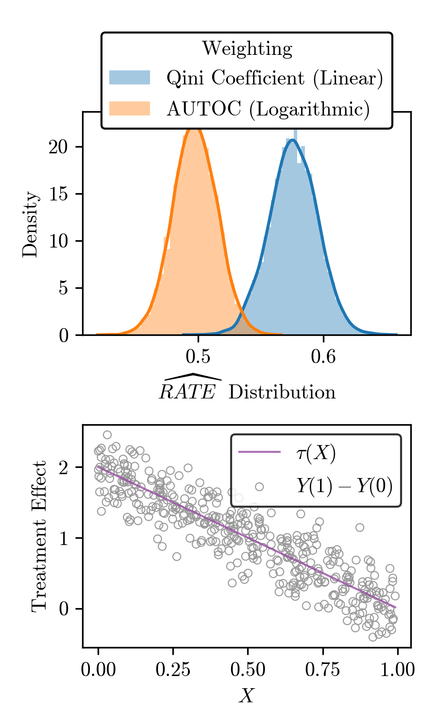
(a) 100% have $|\tau(X_{i})|>0$

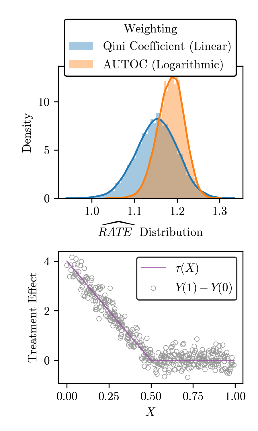
(b) 50% have $|\tau(X_{i})|>0$

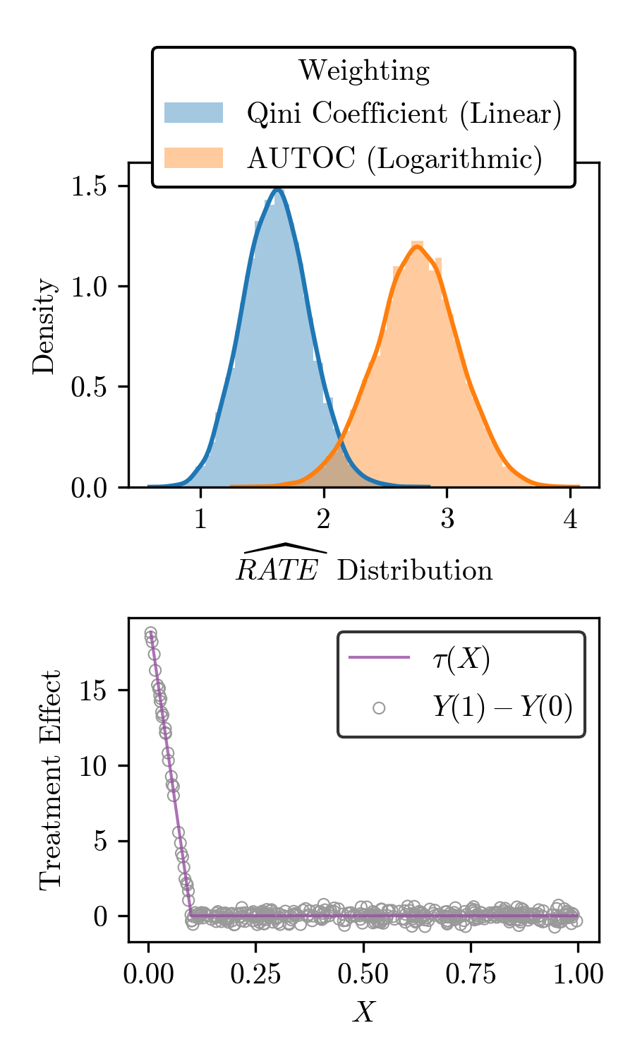
(c) 10% have $|\tau(X_{i})|>0$

Figure 2: Comparison of linear (Qini) vs. logarithmic (AUTOC) weighting functions. If treatment effects are nonzero for a significant proportion of the population (e.g., left figure) the power of the estimated RATE when using linear weighting (Qini) tends to be greater than when using logarithmic (AUTOC) weighting. Conversely, if nonzero treatment effects are concentrated among a small proportion of the population (e.g., right figure) we see that using logarithmic (AUTOC) weighting leads to a greater power for the estimated RATE relative to using linear (Qini) weighting.

For each $p$ in $\{1.0,0.5,0.1\}$, we simulate a dataset and calculate both the AUTOC and Qini metrics using oracle AIPW scores $\Gamma^{\ast}_{i}$ as given in Equation 2.13. Figure 2 shows the distribution of the estimates of each metric over $10000$ Monte Carlo simulations.

When all or a substantial portion (e.g., $>50\%$) of the treatment effects are both heterogeneous and non-zero, using the Qini metric can lead to a higher RATE compared to the AUTOC. However, when only a small subset of individuals have a non-zero heterogeneous treatment effect (e.g., $\leq 10\%$), using the AUTOC can lead to a higher RATE and thus be advantageous. This example highlights a broader intuition about when and why one might choose the AUTOC vs Qini coefficient as a RATE metric: If a researcher believes that only a small subset of their study population experiences nontrivial heterogeneous treatment effects, they should use logarithmic weighting; if they believe that heterogeneous treatment effects are diffuse and substantial across the entire study population, they should use linear weighting. Following this guideline should, in general, increase the statistical power of tests against the absence of heterogeneous treatment effects.

A second important consideration for researchers looking to use RATE metrics concerns how best to generate score estimates, $\widehat{\Gamma}_{i}$, for each individual the evaluation dataset. Here, we focus on choosing a score in the context of data with no unobserved confounding.

As discussed in Section 2.3, both IPW scores and AIPW scores satisfy necessary conditions (Assumption C) for RATE estimation in randomized trials and sometimes do for observational study settings with no unobserved confounding, as well; however, AIPW scores can yield lower variance score estimates in both settings. In a simple experiment, we highlight the significant practical impact of using AIPW score estimates to reduce RATE estimate variance and improve power in a randomized trial.

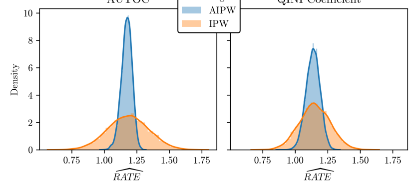
Figure 3: Comparison of RATE estimates obtained using Inverse-Propensity Weighting (IPW) vs. Augmented IPW scores. Using AIPW scores yield RATE estimates with lower variance and greater statistical power compared to RATE estimates using IPW scores.

We consider the same simulation setup as in Section 4. Here, however, instead of using oracle AIPW scores (2.13) to calculate the RATE, we use estimated IPW scores and AIPW scores. In calculating AIPW scores, we use nuisance parameters $\hat{m}(x,w)$ estimated using a random forest regression model with cross-fitting (Chernozhukov et al., 2018b). Thus in each of 10000 Monte Carlo simulations, we generate a synthetic sample according to (4.1), estimate both the AUTOC and Qini coefficient using IPW and AIPW scores on that sample, and compare the final distributions of 10000 RATE point estimates.

Figure 3 shows the resulting distributions. The AIPW score yields lower variance estimates of the RATE compared to the IPW score, consistent with the improved efficiency of AIPW scores for estimating the average treatment effect (Robins et al., 1994). The AIPW score improves the precision of the point estimate and the statistical power of derived hypothesis tests. We recommend using AIPW scores for estimating the RATE in both randomized trial and observational study settings.

5 Aspirin and Stroke

As a first application of RATE, we revisit the International Stroke Trial (IST) introduced in Section 1.1 (Group, 1997; Sandercock et al., 2011). It assessed the treatment effects of Aspirin, Heparin (an anticoagulant), both, or neither for patients with presumed acute ischaemic stroke in a factorial design on 19,435 patients across 36 countries. Primary outcomes included (1) death within 14 days of stroke onset, and (2) death or dependency at 6 months. Follow-up for the primary outcomes was 99% complete. We focus on the outcome of death or dependency at 6 months and restrict our analysis to those patients for whom this outcome was recorded. We also only analyze the effect of Aspirin, irrespective of Heparin assignment status. Consistent with the original trial paper, we employ an intention-to-treat analysis approach (Group, 1997).

We estimate RATE metrics for several prioritization rules on IST, comprising both CATE-based and risk-based approaches. We evaluate

1. A prognostic random forest risk model (Breiman, 2001) trained on individuals assigned to the control arm (this model was used to create quintiles in Figure 1);

2. A logistic regression risk model trained on

3. A causal forest model (Athey et al., 2019) that specifically targets the CATE; and

4. A logistic regression T-learner (Künzel et al., 2019).

Here, treatment effects with a negative sign are desirable (i.e., they correspond to reduced mortality). Our goal is to investigate whether we can identify a subgroup who benefits less than average from aspirin (and so should potentially not be prescribed aspirin), and we hypothesize that patients with a high baseline risk may form such a group. Thus, when evaluating prognostic rules we rank patients with high risk first and when evaluating CATE-based rules we rank patients with positive CATE first. We expect to get a positive RATE in doing so, meaning that we expect to find that patients we believe should benefit less from aspirin in fact do.

In order to avoid overfitting, rules are first trained on a 50% train split, then evaluated on a 50% test split. For each prioritization rule considered, we learn the optimal parameters of the prioritization rule on the train set, and then generate a point estimate and Gaussian half-sample bootstrap 95%-confidence interval for the RATE using 10,000 bootstrap samples from data in the test set. We report associated two-sided $p$-values against the RATE being 0. This test serves as a test against the absence of heterogeneous treatment effects. Given the high (99%) follow-up rate, we simply discarded observations with missing follow-up and did not attempt to correct for censoring. Details on each of these methods can be found in Section C.1.2 of the Supplement and the papers cited above. All prioritization rules are trained and evaluated on the IST data.

Prioritization Rule	AUTOC (95% CI)	$p$-value
Random Forest Risk (grf)	0.014 (0.002, 0.027)	0.022
Logistic Regression Risk	0.011 (0.000, 0.230)	0.057
Causal Forest (grf)	0.006 (-0.012, 0.024)	0.493
Logistic Regression T-learner	0.005 (-0.013, 0.023)	0.588

Table 1: RATE estimates obtained using data from the International Stroke Trial. We also show 95% confidence intervals obtained using the half-sample bootstrap, along with associated $p$-values. The $p$-values are not corrected for multiple testing.

AUTOC estimates from our considered methods, along with 95% confidence intervals, are shown in Table 1. Our first finding is that the AUTOC with prognostic-based targeting (i.e., with the random forest risk model) is statistically significant, with a $p$-value of 0.022. This is an interesting finding since, as discussed in Section 1.1, Group (1997) and Chen et al. (2000) had considered baseline prognostic index as a potential effect modifier; however, their subgroup-based analysis was not powerful enough to obtain statistical significance. Here, in contrast, we find that if we combine machine learning-based estimation of the prognostic index (here using random forests) with RATE-based evaluation, we get significance. In other words, from a statistical point of view, this result highlights the gain in power from using RATE relative to estimating treatment effects separately for different risk quantiles.

6 Prioritization Rules for Antihypertensive Treatment

As a second application of our framework, we consider the problem of personalized antihypertensive treatment. Hypertension, or elevated blood pressure (BP), is implicated in 14% of all deaths across the globe (Fisher and Curfman, 2018) and has a high prevalence around the world (Muntner et al., 2018). Effective hypertension treatment significantly reduces the risk of negative cardiovascular disease outcomes (Psaty et al., 2003). However, it is less clear the degree to which benefits of intensively targeting a low BP with antihypertensive medications are uniform across patients, as antihypertensives carry risks and cause adverse side effects (Group, 2010, 2015).

Here, we study personalized treatment rules for hypertension using two large randomized controlled trials on the effectiveness of intensive blood-pressure control: the Action to Control Cardiovascular Risk in Diabetes Blood Pressure trial (ACCORD-BP) (Group, 2010) and the Systolic Blood Pressure Intervention Trial (SPRINT) (Group, 2015). The ACCORD-BP and SPRINT trials share many similarities such as the treatment (intensive blood-pressure control, which aims for SBP $<120$ mm Hg vs. standard blood-pressure control, which aims for SBP $<140$ mm Hg), study population (see Section D.1 of the Supplementary Materials), and primary outcomes (e.g., myocardial infarction, stroke, death from cardiovascular causes). However, the trials differ in two key aspects: (1) The ACCORD-BP trial was conducted on participants with type 2 diabetes, while SPRINT was conducted on participants without diabetes; and (2) the ACCORD-BP trial found that risk reduction under the intensive blood-pressure treatment arm was non-significant (12%, 95% CI -6% to 27%), while the SPRINT trial found that intensive blood-pressure treatment led to significantly lower risk relative to controls (25% , 95% CI 11% to 36%). The literature has hypothesized that the differences in reported significance of treatment effects may be due to treatment effect heterogeneity (Beddhu et al., 2018; Basu et al., 2017; Kaul, 2017). This is a hypothesis we can test using the RATE. Baseline characteristics for study participants are given in Table 6 of the Supplementary Material.

We use RATE to study the ability of a number of prioritization rules (i.e., $S$ in our notation, as per Definition 1 in Section 2) to identify patients who benefit more than average from intensive blood pressure medication in SPRINT and ACCORD-BP. First, we consider two risk scores for cardiovascular disease that are widely used in clinical practice: The Framingham Risk Score (D’Agostino et al., 2008) and the ACC/AHA Pooled Cohort Equations (Goff et al., 2014). Second, we consider prioritization based on a risk score we trained ourselves via a random forest. Finally we consider two prioritization rules based on CATE estimates, one that fits CATE via Cox proportional hazards regression using what Künzel et al. (2019) called the S-learner approach, and another that fits CATE using causal survival forests (Cui et al., 2023).

We estimate RATE separately in the ACCORD-BP and SPRINT trials. Whenever we use scoring rules that we fit ourselves (i.e., based on forests or Cox regression), we follow the approach of Basu et al. (2017) and train models on the other trial than the one we are estimating a RATE on (e.g., we evaluate a causal survival forest trained with ACCORD-BP on SPRINT, and vice-versa). We produce a 95% confidence intervals and associated two-sided $P$-values as in Section 5. Unlike in the IST discussed above, both the ACCORD-BP and SPRINT trials had non-negligible loss to follow-up (94.6% were lost to follow-up in SPRINT, 85.2% in ACCORD-BP) and so we used right-censored time-to-event outcomes throughout; see Section A.3 of the Supplementary Materials for details.

Table 2 shows results from training prioritization rules on ACCORD-BP and evaluating them on SPRINT, and Table 3 for training on SPRINT and evaluating on ACCORD-BP. In this experiment, the estimated RATE metrics for all risk-based prioritization rules were not significantly different from zero when evaluated on both ACCORD-BP and SPRINT. These findings suggest that, for these two trial populations, the risk-based estimators in consideration would not order patients in accordance with estimated treatment benefit. Additionally, the estimated RATE prioritization rules that directly target the CATE (the Causal Survival Forest and Cox Proportional Hazards S-Learner) were not significantly different from 0 at level $\alpha=0.05$ in both ACCORD-BP and SPRINT, using Gaussian half-sample bootstrap confidence intervals.

Prioritization Rule	AUTOC (95% CI)	$p$-value
Causal Survival Forest (grf)	2.37 (-3.52, 8.27)	0.43
Cox PH S-learner	3.57 (-1.92, 9.07)	0.20
Random Survival Forest Risk (grf)	4.21 (-2.46, 10.88)	0.22
Framingham Risk Score	1.83 (-4.28, 7.94)	0.55
ACC/AHA Pooled Cohort Equations	-1.76 (8.26, 4.73)	0.59

Table 2: AUTOC estimates obtained using data from SPRINT ($n=9069$), with prioritization rules trained on ACCORD ($n=4535$), if necessary. We also show 95% confidence intervals obtained using the half-sample bootstrap, along with associated $p$-values.

Prioritization Rule	AUTOC (95% CI)	$p$-value
Causal Survival Forest (grf)	-5.29 (-17.58, 7.00)	0.40
Cox PH S-learner	8.90 (-2.62, 20.43)	0.13
Random Survival Forest Risk (grf)	2.93 (-8.82, 14.67)	0.62
Framingham Risk Score	-7.01 (-18.45, 4.48)	0.25
ACC/AHA Pooled Cohort Equations	-1.43 (-13.22, 10.36)	0.81

Table 3: AUTOC estimates obtained using data from ACCORD ($n=4535$), with prioritization rules trained on SPRINT ($n=9069$), if necessary. We also show 95% confidence intervals obtained using the half-sample bootstrap, along with associated $p$-values.

Our findings show no significant evidence of heterogeneous treatment effects in the SPRINT and ACCORD-BP trials in terms of the restricted mean survival time (RMST). We also assessed the RATE using a combined version of the SPRINT/ACCORD-BP data, but these results were similarly not significant (see Section D.2 of the Supplementary Materials).

From the results on these data, it remains ambiguous whether or not clinical use of risk scores like the Framingham Risk Score to guide blood pressure control treatment is in fact more beneficial than simply using the original trial’s inclusion/exclusion protocols to guide treatment (given that treatment benefit was significant in SPRINT for the primary outcome). It also remains ambiguous whether there is significant treatment effect heterogeneity at all in these trial populations. Our main results suggest that the SPRINT/ACCORD-BP results are not well-enough powered to support conclusive claims of treatment effect heterogeneity using an RMST outcome. However, we also note contemporaneous work (Oikonomou et al., 2022; Xu et al., 2023) that obtain (marginally) significant detections for heterogeneity in absolute-risk-difference outcomes. Overall, these results highlight the fragility of any claims regarding treatment effect heterogeneity in these trials and demonstrates the importance of having a principled approach towards performing such tests. The RATE provides such a principled approach for evaluating and comparing prioritization rules, as well as testing for global treatment effect heterogeneity.

7 Application to Uplift Modeling

Finally, to demonstrate versatility of the RATE approach outside of the medical domain, we also briefly consider an application to marketing. Traditionally, marketing offers have been targeted based on analogues to risk modeling (e.g., target retention offers to customers predicted to be at risk of canceling the service); however, there has been interest in methods based on CATE estimation, or uplift modeling (Ascarza, 2018; Radcliffe, 2007; Radcliffe and Surry, 1999). One driver of recent interest in CATE estimation is that randomized trials are particularly easy to design and implement the world of digital marketing, and many tools exist to help data scientists run these experiments (Hohnhold et al., 2015; Johnson et al., 2017; Gordon et al., 2019).

We use RATE to compare different targeting rules on a large benchmark dataset released by Criteo for studying uplift modeling in online digital advertising, based on anonymized results from a number of randomized controlled trials on incrementality (Diemert et al., 2018). For the purposes of anonymization, the features released are a random projection of the user features into a 12-dimensional space. The data also contain a binary indicator for treatment status, and two outcomes, visiting the site following the ad, and further conversion into a customer.

	Full data		Training subsample		Test subsample
	Visit	Conversion	Visit	Conversion	Visit	Conversion
Treatment	0.0485	0.0031	0.0492	0.0031	0.0488	0.0031
Control	0.0382	0.0019	0.0395	0.0019	0.0377	0.0021

Table 4: Visit and conversion rates in each arm of the Criteo Uplift Benchmark dataset, and our two randomly subsampled datasets for training and testing uplift models. Tests for difference in means between the rates of the three samples are insignificant at $5\%$-level.

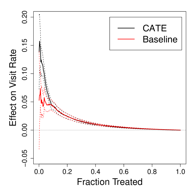
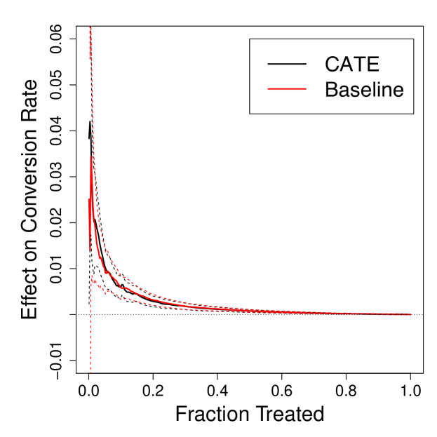
Figure 4: TOC curves for two prioritization rules (baseline- and CATE-based) and two outcomes (rate of visits and rate of conversion) on Criteo Uplift benchmark dataset.

We considered two random-forest based prioritization rules, one fit to the baseline probability of the outcome if untreated (ie., how likely is the user to visit or convert without any advertising), and one fit using causal forests for the conditional average treatment effect. We will call these the baseline and CATE prioritization rules, respectively. The data contain 25,309,483 samples with an unbalanced fraction of treated vs control units; however, we randomly selected two sets of 320,000 samples without replacement, each equally balanced with 160,000 treated and 160,000 control units. We used the first set for training prioritization rule models, and the second set for evaluating the RATE metrics of the learned models. The average visit and conversion rates in the treatment and control arms of the updated dataset and our subsamples are reported in Table 4.

	AUTOC (95% CI)		Qini coefficient (95% CI)
	Visit	Conversion	Visit	Conversion
Baseline	0.0136 (0.0111, 0.0161)	0.0023 (0.0011, 0.0035)	0.0059 (0.0048, 0.0069)	0.00074 (0.00047, 0.00101)
CATE	0.0171 (0.0148, 0.0194)	0.0025 (0.0015, 0.0035)	0.0058 (0.0049, 0.0067)	0.00070 (0.00044, 0.00096)

Table 5: RATE metrics on Criteo Uplift Benchmark dataset. Confidence intervals are estimated using the half-sample bootstrap.

Figure 4 shows the TOC curves for each of the prioritization rules for each of the outcomes, and Table 5 shows the RATE metrics (AUTOC and Qini coefficient) summarizing these curves, along with their confidence intervals. Both methods on both outcomes work better than random prioritization, with strictly positive CIs. For visits, the AUTOC for the CATE-based prioritization rule is marginally higher than the baseline-based rule; the difference between their AUTOC statistics is 0.0034 (95% CI 0.0019, 0.0049), which is a relative increase in AUTOC of 25%. However, the Qini coefficient and the results for conversions are not significantly different between the two prioritization rules. Looking at the TOC curves in Figure 4 gives suggestions as to why this is the case. We see that the average treatment effect among the highest prioritized individuals according to the CATE-based rule is much higher than for the baseline-based rule at similar fractions treated. However, the difference disappears once the fraction treated is more than 10%. The Qini coefficient weights the TOC by the fraction treated, so it downweights the importance of these small groups with large treatment benefit. On the other hand, these groups are more influential in the AUTOC, explaining why we observe a statistically significant difference in this metric. Note that while the confidence intervals overlap between the two metrics, paired bootstrapping is more precise and detects a significant contrast for the AUTOC.

8 Discussion

We discussed evaluation of treatment prioritization rules using a number of metrics motivated by the Area under the Receiver-operating Characteristic curve (AUROC) for classification (Green et al., 1966; Zweig and Campbell, 1993). Our approach enables threshold-agnostic evaluation and comparison of risk-based and CATE-based estimators alike. Researchers can use RATE metrics and half-sample bootstrap confidence intervals to (1) evaluate whether a prioritization rule performs significantly better than chance/random treatment allocation in stratifying subjects according to estimated treatment benefit; (2) directly, meaningfully, and rigorously compare the targeting performance of two different prioritization rules and determine whether one exhibits significant superiority; and (3) perform a global test for the presence of predictable heterogeneous treatment effects, by coupling estimation of the RATE with a powerful, flexible, non-parametric CATE estimator as the prioritization rule. Our approach works in the context of binary outcomes, continuous, real-valued outcomes, and right-censored time-to-event outcomes, making it a practical tool for a number of different fields of study, from marketing and business to medicine and public policy. Additionally, it generalizes existing estimators of the Qini score (Radcliffe, 2007) and AUTOC (Zhao et al., 2013) to any setting where an identification strategy allows the construction of a CATE score, including observational studies with unconfoundedness. The representation of these metrics as a weighted average treatment effect that we provide in (2.4) implies that these metrics will be similar to the average treatment effect in terms of their sensitivity to model misspecification or unobserved confounding.

To apply a treatment prioritization rule in practice, one must convert the prioritization rule into a policy for whom to intervene on versus not. From this perspective, it’s intuitive to consider directly evaluating the prioritization rule on the average reward of the policy implied by thresholding the prioritization rule at a specified level. The implied policy value of treating the top $u$-th of units can be measured using the “high-vs-others” estimator as discussed in Section 2. This estimator is a RATE and so the tools for inference as discussed in Section 3 apply. If the threshold—e.g. treat with antihypertensive medications with 10-year risk of ASCVD $\geq 10\%$—is known at the time of evaluation, this is a reasonable approach. This can also be a reasonable approach if the author has expert knowledge (e.g., regarding the treatment and study population) that would justify assigning weights for all units other than the top $u$-th a weight of zero in calculating the RATE.

However, in many cases, the policy is unclear or may still be subject to change at the time that the prioritization rule is designed. For instance, in healthcare applications, the policy for treatment decisions might additionally depend on individualized risk of serious adverse events from the treatment, patient and provider preferences, costs, and more. In marketing applications, they may depend on varying costs associated with advertising, concerns for advertisement blindness (Hohnhold et al., 2015) and other considerations.

Figure 5: A flowchart for choosing the best evaluation metric to use in an application.

RATE metrics provide a way to summarize the quality of a treatment prioritization rule in ranking units according to potential without specifying a particular treatment policy. This can be especially beneficial when evaluating the degree to which risk-based and other non-centered targeting algorithms optimize treatment benefit. Choosing the appropriate RATE metric for a problem is important. As noted in Section 4, the precision (and thus, statistical power) of a RATE metric depends on the weighting scheme and the shape of the true, underlying TOC curve. In applications where the analyst anticipates that the prioritization rule will be used to find a relatively small group of individuals with a large treatment benefit, they should use the AUTOC curve; the digital advertising example in Section 7 illustrates the practical impacts here. However, in cases where treatment effects are more evenly spread out over the population, the Qini coefficient might be more powerful. From our experience so far working with these metrics, we recommend starting with the AUTOC metric if one is unsure which would be more appropriate. We summarize the above discussions of how to choose an effective metric for heterogeneous treatment effects in applications as a flowchart in Figure 5.

Supplementary Material

Appendix A Additional Results

A.1 Converse to Proposition 2

Proposition 9.

Suppose that $S(X_{i})$ has no ties, i.e., that $F_{S}(X_{i}))$ has a uniform distribution on $[0,\,1]$, and that $\tau(x)=\mathbb{E}[Y_{i}(1)-Y_{i}(0)\,\big{|}\,X_{i}=x]$ is uniformly bounded. Furthermore, suppose that $w\mathrel{\mathop{\mathchar 58\relax}}[0,\,1]\rightarrow\mathbb{R}$ admits a (Radon-Nikodym) derivative $w^{\prime}(u)$ such that $w^{\prime}(u)(1-u)$ is absolutely integrable with respect to Lebesgue measure on $[0,\,1]$, and that $\int_{0}^{1}w(u)\ du=0$. Then $\eta_{w}(S)$ as defined in (2.6) is a RATE in the sense of Definition 3, with the weight function

$$\eta_{w}(S)=\theta_{\alpha_{w}}(S),\ \ \ \ \alpha_{w}(t)=-tw^{\prime}(1-t).$$

Proof    We first note that, by the chain rule, $\eta_{w}=\mathbb{E}[w\left(1-F_{S}(S(X_{i}))\right)\tau(X_{i})]$, and furthermore

$$\eta_{w}(S) =\int w\left(1-F_{S}(S(x))\right)\tau(x)\,d\mathbb{P}(x)$$

$$=w(1)\mathbb{E}\left[\tau(X)\right]-\int\int_{0}^{F_{S}(S(x))}w^{\prime}(1-u)\,du\,\tau(x)\,d\mathbb{P}(x)$$

$$=w(1)\mathbb{E}\left[\tau(X)\right]-\int\int_{0}^{1}1\left(\left\{u\leq F_{S}(S(x))\right\}\right)w^{\prime}(1-u)\,du\,\tau(x)\,d\mathbb{P}(x).$$

Next, because $(1-u)w^{\prime}(u)$ is absolutely integrable and $\tau(x)$ (and thus also the TOC) is uniformly bounded, we can use Fubini’s theorem to continue, and verify that

$$\eta_{w}(S) =w(1)\mathbb{E}\left[\tau(X)\right]-\int_{0}^{1}w^{\prime}(1-u)\int 1\left(\left\{u\leq F_{S}(S(x))\right\}\right)\tau(x)\,d\mathbb{P}(x)\,du$$

$$=w(1)\mathbb{E}\left[\tau(X)\right]-\int_{0}^{1}w^{\prime}(1-u)\left(1-u\right)\left(\operatorname{TOC}(u;\,S)+\mathbb{E}\left[\tau(X)\right]\right)\,du$$

$$=\theta_{\alpha_{w}}(S)+\mathbb{E}\left[\tau(X)\right]\left(w(1)-\int_{0}^{1}w^{\prime}(1-u)\left(1-u\right)\,du\right),$$

where $\theta_{\alpha_{w}}(S)$ is as in Definition 3. Finally, integrating by parts, we see that $\int_{0}^{1}w^{\prime}(1-u)\left(1-u\right)\,du=\int_{0}^{1}w^{\prime}(u)u\,du=w(1)-\int_{0}^{1}w(u)\,du=w(1)$ because $\int_{0}^{1}w(u)\,du=0$ by assumption, and so $\eta_{w}(S)=\theta_{\alpha_{w}}(S)$. ∎

A.2 Tiebreaking

So far, we have assumed that the priority score $S(\cdot)$ provides a strict priority ranking. In many settings of interest, however, $S(\cdot)$ may have ties. In these cases, we break ties by considering all possible permutations of orderings within each set of tied observations, and then averaging the resulting TOC estimates. Thus, in the presence of ties, our definition of the TOC from (2.2) generalizes to

$$\begin{split}&\operatorname{TOC}(u;\,S)=\frac{P(S(X_{i})>q_{u})}{u}\mathbb{E}\left[Y_{i}(1)-Y_{i}(0)\,\big{|}\,S(X_{i})>q_{u}\right]\\ &\quad\,\quad\,\quad+\left(1-\frac{P(S(X_{i})>q_{u})}{u}\right)\mathbb{E}\left[1\left(\left\{S(X_{i})=q_{u}\right\}\right)\left(Y_{i}(1)-Y_{i}(0)\right)\right]\\ &\quad\,\quad\,\quad-\mathbb{E}\left[Y_{i}(1)-Y_{i}(0)\right],\end{split}$$ (A.1)

where $q_{u}=\sup\{q\mathrel{\mathop{\mathchar 58\relax}}F_{S}(q)\leq u\}$. Notice that when there are no ties, so that $P(S(X_{i})>q_{u})=u$, this simplifies to the previous expression for the TOC. Similarly, the sample-average TOC estimator (2.8) averages the $\widehat{\Gamma}_{i}$ across tied observations: If $S(X_{i(k)})>S(X_{i(k+1)})=\ldots=S(X_{i(k^{\prime})})$ for some $k<m<k^{\prime}$, then

$$\widehat{\operatorname{TOC}}\left(\frac{m}{n};s\right)=\frac{1}{m}\left(\sum_{j=1}^{k}\widehat{\Gamma}_{i(j)}+\frac{m-k}{k^{\prime}-k}\sum_{j=k+1}^{k^{\prime}}\widehat{\Gamma}_{i(j)}\right)-\frac{1}{n}\sum_{i=1}^{n}\widehat{\Gamma}_{i}.$$ (A.2)

Given these these tie-robust definitions of the TOC, our definition of the RATE and as associated estimator (2.9) remain as is.

The weighted ATE representation in (2.4) can also be adapted by taking the average of the weights over all possible tie-breaking orders. That is, by replacing $w(t)$ at any $t$ with $P(S(X_{i})=t)=v>0$ with its average over the ties,

$$\frac{1}{v}\int_{0}^{v}w(F_{S}(t)-\epsilon)\operatorname{d}{\epsilon}.$$

Similarly, for the empirical estimate, by replacing $w(m/n)$ at any $k<m<k^{\prime}$ with $S(X_{m})=S(X_{k^{\prime}})$ with

$$\frac{1}{k^{\prime}-k}\sum_{j=k+1}^{k^{\prime}}w\left(j/n\right).$$

A.3 A Score for Time-to-event Outcomes

The AIPW approach for both randomized trials and observational studies can be generalized to handle time-to-event outcomes with right-censored outcomes. To do so, we first need to introduce some additional notation to specify the event times and censoring times. We denote the counterfactual event times as $T_{i}(1)$ and $T_{i}(0)$, and the counterfactual censoring times as $C_{i}(1)$ and $C_{i}(0)$. With censored data, we only observe the factual event time $T_{i}=T_{i}(W_{i})$ up to the factual censoring time $C_{i}=C_{i}(W_{i})$. That is, the observed data are $U_{i}=\min\{T_{i},C_{i}\}$ and $\Delta_{i}=1\{U_{i}=T_{i}\}$.

Two endpoints that are often used with time-to-event outcomes can be easily adapted to the methods developed here. To study absolute risk, we use the outcome

$$Y_{i}(w)=1\{T_{i}(w)\leq t_{0}\},$$

and to study the restricted mean survival time, we use

$$Y_{i}(w)=\min\{T_{i}(w),t_{0}\},$$

for a pre-specified time $t_{0}$ that denotes the end of observation. The causal effect estimated in each case is the absolute risk reduction

$$P\left(T_{i}(1)\leq t_{0}\,\big{|}\,X_{i}=x\right)-P\left(T_{i}(0)\leq t_{0}\,\big{|}\,X=x\right),$$

and the difference in restricted mean survival time,

$$\mathbb{E}\left[\min\{T_{i}(1),t_{0}\}-\min\{T_{i}(0),t_{0}\}\,\big{|}\,X=x\right].$$

With either of these endpoints, we use the augmented IPW approach described in Tsiatis (2007), based off of the construction from Robins et al. (1994), and used as a score for CATE estimation in Cui et al. (2023). For either of these endpoints, the score is the same. Let $\tilde{U}_{i}=\min\{U_{i},t_{0}\}$, $\tilde{\Delta}_{i}=1\{U_{i}=T_{i}~{}\text{or}~{}C_{i}>t_{0}\}$ and $Y_{i}=Y_{i}(W_{i})$ as defined above for each endpoint. Then, the score is

$$\widehat{\Gamma}_{i}=\hat{m}(X_{i},1)-\hat{m}(X_{i},0)+\frac{W_{i}-\hat{e}(X_{i})}{(1-\hat{e}(X_{i}))\hat{e}(X_{i})}\left(\frac{\tilde{\Delta}_{i}Y_{i}-\left(1-\tilde{\Delta}_{i}\right)\hat{q}(\tilde{U}_{i},X_{i},W_{i})}{\hat{S}_{C}(\tilde{U}_{i},X_{i},W_{i})}\right.$$ (A.3)

$$\quad~{}\quad\left.-\int_{0}^{\tilde{U}_{i}}\frac{\hat{q}(s,X_{i},W_{i})}{\hat{S}_{C}(s,X_{i},W_{i})}\operatorname{d}{\hat{\Lambda}}_{C}(s,X_{i},W_{i})-\hat{m}(X_{i},W_{i})\right),$$

with

$$m(x,w)=\mathbb{E}\left[Y_{i}\,\big{|}\,X_{i}=x,W_{i}=w\right],$$

$$q(u,x,w)=\mathbb{E}\left[Y_{i}\,\big{|}\,X_{i}=x,U_{i}\geq u,W_{i}=w\right],~{}\mbox{and}$$

$$S_{C}(s,x,w)=P(C_{i}\geq s\,\big{|}\,X_{i}=x,W_{i}=w).$$

Similarly to the observational study setting, $\hat{e},$ $\hat{m}$, $\hat{q}$, and $\hat{S}_{C}$ refer to nonparametrically estimated versions of the corresponding functions defined without a $\hat{~{}}$. The oracle score $\Gamma_{i}^{\ast}$ is the equivalent with all of the estimated functions replaced with their corresponding true function.

A.4 Hypothesis Testing and Confidence Intervals

An important aspect of RATE metrics is that they provide a natural null hypothesis for testing whether a prioritization rule is useful for identifying subpopulations with heterogeneous treatment effects. Consider the null hypothesis $H_{0}$: $\theta_{\alpha}(S)\leq 0$. A test of this hypothesis is sensitive to treatment heterogeneity aligned with the prioritization rule $S$.

Additionally, a test of $H_{0}$ can be interpreted as a test of treatment effect heterogeneity. If there is no treatment effect heterogeneity, meaning that $\tau(X)=\tau$ is constant, then $\operatorname{TOC}(u;S)=0$ for any $u\in(0,1]$, and so $\theta_{\alpha}(S)=0$. However, it will not be a powerful test for treatment effect heterogeneity without a good prioritization rule. The statistic $\theta_{\alpha}(S)$ can be zero if there is no treatment effect heterogeneity, or if the prioritization rule $S$ has no relationship with the heterogeneous treatment effects. Some may find it advantageous, that instead of simply testing whether heterogeneous treatmenet effects exist, it tests whether the treatment effect is predictable by some prioritzation rule. However, those interested in studying whether heterogeneous treatment effects exist regardless of whether or not they can be identified by a prioritization rule should consider tests such as Ding et al. (2016).

Using the sampling distribution for $\widehat{\theta}$ from Section 3, we can easily develop a valid test for $H_{0}$ using the bootstrap. Let $\sigma^{\ast}$ denote the standard deviation of the bootstrap estimates $\widehat{\theta}^{\ast}$. Then, an asymptotically valid $P$-value for $H_{0}$ is

$$2\Phi\left(-\frac{|\widehat{\theta}|}{\sigma^{\ast}}\right),$$

where $\Phi$ is the CDF of the unit normal distribution, $\mathsf{N}{}(0,1).$ Similarly, we can use the sampling distribution to derive asymptotically valid confidence intervals for $\theta_{\alpha}(S)$. To get a $1-\alpha$ confidence interval, we can use

$$\widehat{\theta}\pm z_{1-\alpha/2}\sigma^{\ast},$$

where $z_{1-\alpha/2}=\Phi^{-1}(1-\alpha/2)$, and, as above, $\sigma^{\ast}$ is the standard deviation of the bootstrap estimates $\widehat{\theta}^{\ast}$.

Appendix B Proofs

B.1 Proof of Proposition 2

Proof    Let $A=\int_{0}^{1}\alpha(u)\ du.$ Now, note that

$$\theta_{a}(S) =\int_{0}^{1}\alpha(u)\mathbb{E}\left[Y_{i}(1)-Y_{i}(0)\,\big{|}\,F_{S}(S(X_{i}))\geq 1-u\right]\operatorname{d}{u}-A\mathbb{E}\left[Y_{i}(1)-Y_{i}(0)\right]$$

$$=\int_{0}^{1}\frac{\alpha(u)}{u}\mathbb{E}\left[\left(Y_{i}(1)-Y_{i}(0)\right)1\left(\left\{F_{S}(S(X_{i}))\geq 1-u\right\}\right)\right]\operatorname{d}{u}-A\mathbb{E}\left[Y_{i}(1)-Y_{i}(0)\right]$$

$$=\int_{0}^{1}\frac{\alpha(u)}{u}\mathbb{E}\left[\tau(X_{i})1\left(\left\{F_{S}(S(X_{i}))\geq 1-u\right\}\right)\right]\operatorname{d}{u}-A\mathbb{E}\left[Y_{i}(1)-Y_{i}(0)\right].$$

By recalling that we assumed $$\tau(X) \frac{\alpha(u)}{u} 1\geq u\geq 1-F_{S}(S(X_{i})) S(X_{i})$$ is uniformly bounded and is absolutely integrable on for almost every , we can apply Fubini’s Theorem to get

$$=\mathbb{E}\left[\left(Y_{i}(1)-Y_{i}(0)\right)\int_{0}^{1}\frac{a(u)}{u}1\left(\left\{F_{S}(S(X_{i}))\geq 1-u\right\}\right)\operatorname{d}{u}\right]-A\mathbb{E}\left[Y_{i}(1)-Y_{i}(0)\right]$$

$$=\mathbb{E}\left[\left(Y_{i}(1)-Y_{i}(0)\right)\int_{1-F_{S}(S(X_{i}))}^{1}\frac{a(u)}{u}\operatorname{d}{u}\right]-A\mathbb{E}\left[Y_{i}(1)-Y_{i}(0)\right].$$

∎

B.2 Proof of Theorem 3

Proof    Let $\widehat{F}_{S}(q^{-})$ denote the empirical distribution at the left limit, instead of the right, and define $\widehat{G}_{S}(q)=1-\widehat{F}_{S}(q^{-})$, which is the empirical distribution function of the observations in the reverse order. Note that the quantile $j/n$ of the $i(j)$-th example is simply $\widehat{G}_{S}(Q_{i(j)})$. Then, we decompose $\sqrt{n}(\widehat{\theta}-\theta)$ into two leading terms that we show are asymptotically linear, followed by remainder terms that we show vanish under Assumptions A-C.

$$\frac{1}{\sqrt{n}}\sum_{i=1}^{n}w_{n}(\widehat{G}_{S}(Q_{i}))\widehat{\Gamma}_{i}-\theta =\underbrace{\frac{1}{\sqrt{n}}\sum_{i=1}^{n}w(1-F_{S}(Q_{i})(\Gamma^{\ast}_{i}-\overline{\tau}(Q_{i}))}_{\text{Term 1}}$$

$$~{}~{}~{}~{}+\underbrace{\frac{1}{\sqrt{n}}\sum_{i=1}^{n}w(\widehat{G}_{S}(Q_{i}))\overline{\tau}(Q_{i})-\theta}_{\text{Term 2}}$$

$$~{}~{}~{}~{}+\underbrace{\frac{1}{\sqrt{n}}\sum_{i=1}^{n}(w_{n}(\widehat{G}_{S}(Q_{i}))-w(\widehat{G}_{S}(Q_{i})))\overline{\tau}(Q_{i})}_{\text{Term 3}}$$

$$~{}~{}~{}~{}+\underbrace{\frac{1}{\sqrt{n}}\sum_{i=1}^{n}(w_{n}(\widehat{G}_{S}(Q_{i}))-w(1-F_{S}(Q_{i})))(\Gamma^{\ast}_{i}-\overline{\tau}(Q_{i}))}_{\text{Term 4}}$$

$$~{}~{}~{}~{}+\underbrace{\frac{1}{\sqrt{n}}\sum_{i=1}^{n}w_{n}(\widehat{G}_{S}(Q_{i}))\delta_{i}.}_{\text{Term 5}}$$

Term 1

The first term is trivially a sum of iid random variables.

Term 2

The second term (which we will denote as $T_{n}$) is an $L$-statistic (van der Vaart, 1998; Shorack and Wellner, 2009) with $\overline{\tau}(q)$ of bounded variation. To show that it is asymptotically linear, we use the following assumptions and theorem from Shorack and Wellner (2009):

Assumption D.

[Assumption 1, Shorack and Wellner (2009)] (a) The weight function $w\mathrel{\mathop{\mathchar 58\relax}}(0,1)\to\mathbb{R}$ satisfies $|w(1-t)|\leq B(t)=Mt^{-b_{1}}(1-t)^{-b_{2}}$ for $M<\infty$ and $\max\{b_{1},b_{2}\}<1$, and (b) $\overline{\tau}(q)=\overline{\tau}_{+}(q)-\overline{\tau}_{-}(q)$, each monotone non-decreasing, with $|\overline{\tau}_{\pm}(F_{S}^{-1}(t))|\leq D(t)=Mt^{-d_{1}}(1-t)^{-d_{2}}$.

Assumption E.

[Assumption 2’, Shorack and Wellner (2009)] (a) $w$ has a continuous derivative on $(0,1)$ satisfying $|w^{\prime}(1-t)|\leq\frac{B(t)}{t(1-t)}$ for $B$ defined as in Assumption D.

Theorem 10.

[Theorem 1, Shorack and Wellner (2009)] Suppose Assumptions D and E hold with $\alpha=\max\{b_{1}+d_{1},b_{2}+d_{2}\}<1/2$. Then,

$$\sqrt{n}(T_{n}-\theta)=-\int_{0}^{1}w(1-t)\mathbb{U}_{n}(t)\operatorname{d}{h(F_{S}^{-1}(t))}+o_{P}(1).$$

Assumption D(a) follows directly from Assumption A. From Assumption B, we know that $\overline{\tau}(q)$ is of bounded variation, and that $\mathbb{E}[|\overline{\tau}(Q)|^{r}]<\infty$, which implies that we can write $\overline{\tau}(q)=\overline{\tau}_{+}(q)-\overline{\tau}_{-}(q)$, with $\mathbb{E}[|\overline{\tau}_{\pm}(Q)|^{r}]<\infty$. Now, Markov’s inequality implies that for $s>0$,

$$P(|\overline{\tau}_{\pm}(Q)|\geq s)\leq\frac{\mathbb{E}[|\overline{\tau}_{\pm}(Q)|^{r}]}{s^{r}}.$$

Inverting this statement, using the fact that $q\mapsto\overline{\tau}_{\pm}(q)$ is monotone, we see that Assumption D(b) holds with $d_{1}=d_{2}=1/r$. As stipulated in Assumption B, $\alpha=1/r+b<1/2$. Therefore, $T_{n}$ satisfies the assumptions of Theorem 10, implying that it is asymptotically linear with influence function

$$Y_{i}=\int_{Q_{i}}^{\infty}w(1-F(q))\operatorname{d}{\overline{\tau}(q)}-\theta.$$

The rest of the proof involves showing the remaining terms are asymptotically negligible.

Term 3

For any fixed $\epsilon>0$, applying Markov’s inequality followed by Hölder’s inequality gives

$$P\left(\bigg{|}\frac{1}{\sqrt{n}}\sum_{i=1}^{n}\left(w_{n}(\widehat{G}_{S}(Q_{i}))-w(\widehat{G}_{S}(Q_{i}))\right)\overline{\tau}(Q_{i}))\bigg{|}\geq\epsilon\right)$$

$$~{}~{}~{}~{}~{}\leq\frac{\mathbb{E}\left[\bigg{|}\sum_{i=1}^{n}\left(w_{n}(\widehat{G}_{S}(Q_{i}))-w(\widehat{G}_{S}(Q_{i}))\right)\frac{\overline{\tau}(Q_{i})}{\sqrt{n}}\bigg{|}\right]}{\epsilon}$$

$$~{}~{}~{}~{}~{}\leq\frac{\mathbb{E}\left[\left(\sum_{i=1}^{n}\left(w_{n}(\widehat{G}_{S}(Q_{i}))-w(\widehat{G}_{S}(Q_{i}))\right)^{p}\right)^{1/p}\left(\frac{1}{n^{r/2}}\sum_{i=1}^{n}|\overline{\tau}|^{r}(Q_{i})\right)^{1/r}\right]}{\epsilon}$$

Assumption A gives that $\left(\sum_{i=1}^{n}\left(w_{n}(\widehat{G}_{S}(Q_{i}))-w(\widehat{G}_{S}(Q_{i}))\right)^{p}\right)<C$ eventually. Applying Jensen’s inequality shows that $\mathbb{E}\left[\left(\frac{1}{n}\sum_{i=1}^{n}|\overline{\tau}|^{r}(Q_{i})\right)^{1/r}\right]\leq\mathbb{E}[\overline{\tau}^{r}(Q_{i})]^{1/r}$, which is bounded by Assumption B. Therefore, the numerator is $O(n^{1/2-1/r})=o(1)$.

Term 4

For any fixed $\epsilon>0$, applying Chebyshev’s inequality conditionally on $\{Q_{i}\}_{i=1}^{n}$ shows that the fourth term satisfies

$$P\left(\bigg{|}\frac{1}{\sqrt{n}}\sum_{i=1}^{n}\left(w_{n}(\widehat{G}_{S}(Q_{i}))-w(1-F_{S}(Q_{i}))\right)(\Gamma^{\ast}_{i}-\overline{\tau}(Q_{i}))\bigg{|}\geq\epsilon\right)$$

$$~{}~{}~{}~{}~{}=\mathbb{E}\left[P\left(\bigg{|}\frac{1}{\sqrt{n}}\sum_{i=1}^{n}\left(w_{n}(\widehat{G}_{S}(Q_{i}))-w(1-F_{S}(Q_{i}))\right)(\Gamma^{\ast}_{i}-\overline{\tau}(Q_{i}))\bigg{|}\geq\epsilon\mid\{Q_{i}\}_{i=1}^{n}\right)\right]$$

$$~{}~{}~{}~{}~{}=\mathbb{E}\left[\frac{1}{\epsilon^{2}}{\rm Var}\left(\frac{1}{\sqrt{n}}\sum_{i=1}^{n}\left(w_{n}(\widehat{G}_{S}(Q_{i}))-w(1-F_{S}(Q_{i}))\right)(\Gamma^{\ast}_{i}-\overline{\tau}(Q_{i}))\mid\{Q_{i}\}_{i=1}^{n}\right)\right]$$ (B.1)

$$~{}~{}~{}~{}~{}=\frac{1}{\epsilon^{2}}\mathbb{E}\left[\frac{1}{n}\sum_{i=1}^{n}\left(w_{n}(\widehat{G}_{S}(Q_{i}))-w(1-F_{S}(Q_{i}))\right)^{2}{\rm Var}(\Gamma_{i}^{\ast}\mid Q_{i})\right]$$ (B.2)

$$~{}~{}~{}~{}~{}\leq\frac{C_{g}}{\epsilon^{2}}\mathbb{E}\left[\frac{1}{n}\sum_{i=1}^{n}\left(w_{n}(\widehat{G}_{S}(Q_{i}))-w(1-F_{S}(Q_{i}))\right)^{2}\right],$$

where (B.1) to (B.2) follows from the rule that ${\rm Var}(aX+bY)=a^{2}{\rm Var}(X)+b^{2}{\rm Var}(Y),$ when $X$ and $Y$ are independent, and noting that each term in the sum is independent given $\{Q_{i}\}_{i=1}^{n}$. By assumption, $\mathbb{E}[\tfrac{1}{n}\sum_{i=1}^{n}(w_{n}(\widehat{G}_{S}(Q_{i}))-w(1-F_{S}(Q_{i})))^{2}]\to 0$. The last inequality follows from Assumption B.

Term 5

Finally, we control the last term using Assumption C. We begin by splitting the sum up into the $K$ partitions,

$$\frac{1}{\sqrt{n}}\sum_{i=1}^{n}w_{n}(\widehat{G}_{S}(Q_{i}))\delta_{i}=\sum_{k=1}^{K}\frac{1}{\sqrt{n}}\sum_{i\in I_{k}}w_{n}(\widehat{G}_{S}(Q_{i}))\delta_{i},$$

and note that because these partitions are selected uniformly at random, it suffices to show that

$$P\left(\bigg{|}\frac{1}{\sqrt{n}}\sum_{i\in I_{1}}w_{n}(\widehat{G}_{S}(Q_{i}))\delta_{i}\bigg{|}\geq\epsilon\right)\to 0$$

for any $\epsilon>0$. Recalling $G_{1}$ from Assumption C, we divide this event into a piece that happens on $G_{1}$ and a piece that happens on $G_{1}^{C}$,

$$P\left(\bigg{|}\frac{1}{\sqrt{n}}\sum_{i\in I_{1}}w_{n}(\widehat{G}_{S}(Q_{i}))\delta_{i}\bigg{|}\geq\epsilon\right)\leq P\left(\bigg{|}\frac{1}{\sqrt{n}}\sum_{i\in I_{1}}w_{n}(\widehat{G}_{S}(Q_{i}))\delta_{i}\bigg{|}\geq\epsilon\mid G_{1}\right)P\left(G_{1}\right)+P\left(G_{1}^{C}\right).$$

Because $P(G_{1})\to 1$, we need to show that

$$P\left(\bigg{|}\frac{1}{\sqrt{n}}\sum_{i\in I_{1}}w_{n}(\widehat{G}_{S}(Q_{i}))\delta_{i}\bigg{|}\geq\epsilon\mid G_{1}\right)\to 0.$$

Denote $\{Q_{i}\}_{i\in I_{1}},\{(W_{i},X_{i},Y_{i})\}_{i\not\in I_{1}}$ as $B_{1}$. Using $\stackrel{{\scriptstyle a.s.}}{{\rightarrow}}$ here to denote convergence almost everywhere on $G_{1}$, it suffices to show that

$$P\left(\bigg{|}\frac{1}{\sqrt{n}}\sum_{i\in I_{1}}w_{n}(\widehat{G}_{S}(Q_{i}))\delta_{i}\bigg{|}\geq\epsilon\mid B_{1},G_{1}\right)\stackrel{{\scriptstyle a.s.}}{{\rightarrow}}0,$$

because the bounded convergence theorem implies that conditional convergence implies unconditional convergence.

If we replace $w_{n}(\widehat{G}_{S}(Q_{i}))$ with $w(1-F_{S}(Q_{i}))$ this would follow easily by Chebyshev’s inequality from the bias and variance conditions of Assumption C:

$$|\mathbb{E}\left[\frac{1}{\sqrt{n}}\sum_{i\in I_{1}}^{n}w(1-F_{S}(Q_{i}))\delta_{i}\mid G_{1},B_{1}\right]|\leq|\sqrt{n}\mathbb{E}[w(1-F_{S}(Q_{i}))\delta_{i}\mid B_{1},G_{1}]|\to 0,$$

and, because we assumed in Assumption C that $\{\delta_{i}\}_{i\in I_{1}}$ are independent conditionally on $B_{1},G_{1}$,

$${\rm Var}\left(\frac{1}{\sqrt{n}}\sum_{i\in I_{1}}^{n}w(1-F_{S}(Q_{i}))\delta_{i}\mid G_{1},B_{1}\right) =\frac{1}{n}\sum_{i\in I_{1}}{\rm Var}\left(w(1-F_{S}(Q_{i}))\delta_{i}\mid G_{1},B_{1}\right)\to 0.$$

This, along with the following lemma proves that Term 5 converges to zero.

Lemma 11.

Under Assumptions A and C,

$$P\left(\bigg{|}\frac{1}{\sqrt{n}}\sum_{i\in I_{1}}(w_{n}(\widehat{G}_{S}(Q_{i}))-w(1-F_{S}(Q_{i})))\delta_{i}\bigg{|}\geq\epsilon\mid B_{1},G_{1}\right)\stackrel{{\scriptstyle a.s.}}{{\rightarrow}}0.$$ (B.3)

Proving Lemma 11 is similar to how we control Terms 2-4 in in the above decomposition, however now with an $L$-statistic whose variance goes to 0. See Section B.7 in the Supplementary Materials for the details. ∎

B.3 Proof of Lemma4

Proof    Throughout, we will assume that $n$ is divisible by two for notational simplicity. Because $\sqrt{n}(\widehat{\beta}-\beta)=\frac{1}{\sqrt{n}}\sum_{i=1}^{n}\psi(Z_{i})+o_{P}(1)$, when fit with $n/2$ samples, we have that $\sqrt{n}(\widehat{\beta}^{\ast}-\beta)=\sqrt{n}\frac{2}{n}\sum_{i=1}^{n/2}\psi(Z_{i})+o_{P}(1)$.

Write $\sqrt{n}(\widehat{\beta}^{\ast}-\widehat{\beta})$ as the difference between the two terms above,

$$\sqrt{n}(\widehat{\beta}^{\ast}-\widehat{\beta}) =\sqrt{n}(\widehat{\beta}^{\ast}-\beta)-\sqrt{n}(\widehat{\beta}-\beta)$$

$$=\frac{1}{\sqrt{n}}\sum_{i=1}^{n}V_{i}\psi(Z_{i})+o_{P}(1),$$ (B.4)

where $V_{i}$ is $1$ if the $i$-th example is in the subset of $n/2$ examples in the bootstrap sample, and otherwise is $-1$.

Our goal is to show that this is (conditionally) asymptotically normal with distribution $\mathsf{N}{}(0,{\rm Var}(\psi(Z_{i}))$. Because $\sqrt{n}(\widehat{\beta}-\beta)\stackrel{{\scriptstyle d}}{{\rightsquigarrow}}Z,$ with $Z\sim\mathsf{N}{}(0,{\rm Var}(\psi(Z_{i}))$, this will prove the result.

To show that this is true, we first consider a “binomialized” version of the term (B.4). Let $N_{n}$ be a random draw from a $\operatorname{Ber}(n,\frac{1}{2})$ distribution. If $N_{n}>n/2$, randomly choose $N_{n}-n/2$ samples with $V_{i}=-1$ and set $\tilde{V}_{i}=1$. If $N_{n}<n/2$, randomly choose $n/2-N_{n}$ samples with $V_{i}=1$ and set $\tilde{V}_{i}=-1$. Set $\tilde{V}_{i}=V_{i}$ for all other samples. With this construction, $\{\tilde{V}_{i}\}_{i=1}^{n}$ are i.i.d. Rademacher random variables,

$$\tilde{V}_{i}=\begin{cases}1&\text{w.p.}~{}\frac{1}{2}\\ -1&\text{w.p.}~{}\frac{1}{2}.\end{cases}$$

Therefore, the multiplier central limit theorem (Van Der Vaart and Wellner, 1996, Lemma 2.9.5) implies that

$$\frac{1}{\sqrt{n}}\sum_{i=1}^{n}\tilde{V}_{i}\psi(Z_{i})$$

converges to $\mathsf{N}{}(0,{\rm Var}(\psi(Z_{i}))$, conditionally on $(Z_{i})_{i=1}^{n}$ almost surely.

To complete the proof, we need to show that conditionally (almost surely) on $(Z_{i})_{i=1}^{n}$,

$$R_{n}(N_{n})=\frac{1}{\sqrt{n}}\sum_{i=1}^{n}(\tilde{V}_{i}-V_{i})\psi(Z_{i})=o_{P}(1).$$

Towards this goal, first notice that $V_{i}-\tilde{V}_{i}$ is only nonzero on the $|N_{n}-n/2|$ samples changed in the construction of $\tilde{V}_{i}$. Let $I_{n}$ be the indices of these samples. Then, observe that

$$R_{n}(N_{n})=\operatorname{sign}{}(N_{n}-n/2)\frac{2}{\sqrt{n}}\sum_{i\in I_{n}}\psi(Z_{i}).$$

Inspecting the symmetry of $R_{n}(N_{n})$, we can see that because $N_{n}$ is symmetric about $n/2$, $\widetilde{\mathbb{E}}\left[R_{n}(N_{n})\right]=0$, with $\widetilde{\mathbb{E}}\left[\cdot\right]$ shorthand for $\mathbb{E}\left[\cdot\,\big{|}\,\{Z_{i}\}_{i=1}^{n}\right].$ Our approach, then, is to show that $\widetilde{{\rm Var}{}}{}(R_{n}(N_{n}))\stackrel{{\scriptstyle a.s.}}{{\rightarrow}}0$, where $\widetilde{{\rm Var}{}}{}(\cdot)={\rm Var}(\cdot\mid\{Z_{i}\}_{i=1}^{n})$ which by Chebyshev’s inequality, implies $P(|R_{n}(N_{n})|>\epsilon\,\big{|}\,\{Z_{i}\}_{i=1}^{n})\to 0,$ as claimed.

To bound the variance, we start by applying the law of total variance,

$$\widetilde{{\rm Var}{}}{}(R_{n}(N_{n}))=\widetilde{{\rm Var}{}}{}\left(\widetilde{\mathbb{E}}\left[R_{n}(N_{n})\,\big{|}\,N_{n}\right]\right)+\widetilde{\mathbb{E}}\left[\widetilde{{\rm Var}{}}{}(R_{n}(N_{n})\,\big{|}\,N_{n})\right],$$

and note that conditional on $N_{n}$, the remaining randomness is the choice of $|N_{n}-n/2|$ samples in $I_{n}$. In this way,

$$\sum_{i\in I_{n}}\psi(Z_{i})$$

is naturally interpretable as $A_{n}\mathrel{\mathop{\mathchar 58\relax}}=|N_{n}-n/2|$ times the sample average of $A_{n}$ randomly drawn points $\psi(Z_{i})$ from the finite population $\{\psi(Z_{i})\}_{i=1}^{n}$. With this in mind,

$$\widetilde{\mathbb{E}}\left[\sum_{i\in I_{n}}\psi(Z_{i})\,\big{|}\,N_{n}\right] =\frac{A_{n}}{n}\sum_{i=1}^{n}\psi(Z_{i})$$

$$\widetilde{{\rm Var}{}}{}\left(\sum_{i\in I_{n}}\psi(Z_{i})\,\big{|}\,N_{n}\right) =A_{n}\frac{n-A_{n}}{n}\left(\frac{1}{n-1}\sum_{i=1}^{n}\psi^{2}(Z_{i})-\left(\frac{1}{n-1}\sum_{i=1}^{n}\psi(Z_{i})\right)^{2}\right).$$

Plugging these expressions into $R_{n}(N_{n})$ gives

$$\widetilde{\mathbb{E}}\left[R_{n}(N_{n})\,\big{|}\,N_{n}\right] =\frac{2}{\sqrt{n}}\frac{N_{n}-n/2}{n}\sum_{i=1}^{n}\psi(Z_{i})$$

and so

$$\widetilde{{\rm Var}{}}{}\left(\widetilde{\mathbb{E}}\left[R_{n}(N_{n})\,\big{|}\,N_{n}\right]\right) =\frac{4}{n}\widetilde{{\rm Var}{}}{}(N_{n})\left(\frac{1}{n}\sum_{i=1}^{n}\psi(Z_{i})\right)^{2}=\left(\frac{1}{n}\sum_{i=1}^{n}\psi(Z_{i})\right)^{2}$$ (B.5)

and

$$\widetilde{\mathbb{E}}\left[\widetilde{{\rm Var}{}}{}\left(R_{n}(N_{n})\,\big{|}\,N_{n}\right)\right]=\widetilde{\mathbb{E}}\left[\frac{4A_{n}(n-A_{n})}{n^{2}}\right]\underbrace{\left(\frac{1}{n-1}\sum_{i=1}^{n}\psi^{2}(Z_{i})-\left(\frac{1}{n-1}\sum_{i=1}^{n}\psi(Z_{i})\right)^{2}\right)}_{s_{\psi}^{2}}.$$ (B.6)

Term (B.5) converges to zero almost surely by the Strong Law of Large Numbers. Term (B.6) also converges to zero almost surely, because $(n-A_{n})/n\leq 1$, $\widetilde{\mathbb{E}}\left[A_{n}/n\right]\asymp 1/\sqrt{n}$, and $s_{\psi}^{2}\to{\rm Var}(\psi(Z_{i}))$ almost surely by the Strong Law. ∎

B.4 Proof of Lemma 6

Proof    Define $\widehat{G}_{S}(q)$ as in the proof of Theorem 3 in Section B, and let $G_{S}(q)$ be the corresponding distribution function of $S(X_{i})$ in reverse order. By continuity, we know that $|w(\widehat{G}_{S}(S(X_{i})))-w(1-F_{S}(S(X_{i})))|\leq\rho_{w}(|\widehat{G}_{S}(S(X_{i}))-G_{S}(S(X_{i})|)$, where $\rho_{w}$ is the modulus of continuity of $w$. By the monotonicity of $\rho_{w}$, $\rho_{w}(|\widehat{G}_{S}(S(X_{i})-G_{S}(S(X_{i})|)\leq\rho_{w}(\|\widehat{G}-G\|_{\infty}))$. Therefore, $\frac{1}{n}\sum_{i=1}^{n}(w(\widehat{G}_{S}(S(X_{i})))-w(G_{S}(S(X_{i}))))^{2}\leq\rho_{w}^{2}(\|\widehat{G}-G\|_{\infty})$. The Glivenko-Cantelli Theorem shows that $\|\widehat{G}-G\|_{\infty}\to 0$ almost surely, and so the claimed statement holds due to the bounded convergence theorem, as $\widehat{G}$ and $G$ are bounded in $[0,1]$, implying that $\rho_{w}(\|\widehat{G}-G\|_{\infty})$ is bounded, as well. ∎

B.5 Proof of Proposition 8

Proof    Define $\widehat{G}_{S}(q)$ as in the proof of Theorem 3 in Section B, and let $G_{S}(q)$ be the corresponding distribution function of $S(X_{i})$ in reverse order. Writing

$$\mathbb{E}[\frac{1}{n}\sum_{i=1}^{n}(w_{n}(\widehat{G}_{S}(S(X_{i})))-w(G_{S}(S(X_{i}))))^{2}]$$

$$\leq\frac{2}{n}\underbrace{\sum_{i=1}^{n}(w_{n}(i/n)-w(i/n))^{2}}_{\text{Part 1}}+\underbrace{\mathbb{E}\left[\frac{2}{n}\sum_{i=1}^{n}(-\log(\widehat{G}_{S}(Q_{i}))+\log(G_{S}(Q_{i})))^{2}\right]}_{\text{Part 2}},$$

we verify that each of these terms vanishes in the following steps:

1. Showing that Part 1 is $O(1)$, then

2. showing that Part 2 vanishes.

Step 1: Recall that $w_{n}(i/n)=H_{n}-H_{i}-1$ and $w(i/n)=\log(n)-\log(i)-1$. Noting that $|H_{n}-H_{k}-\log(n)+\log(k)|\leq\frac{1}{2k}$ for $1\leq k\leq n$, averaging over these differences gives

$$\sum_{i=1}^{n}(w_{n}(i/n)-w(i/n))^{2}\leq\sum_{i=1}^{n}\frac{1}{(2i)^{2}}\leq\frac{\pi^{2}}{24}.$$

This verifies the second part of Assumption A. Additionally, $\frac{1}{n}\sum_{i=1}^{n}(w_{n}(i/n)-w(i/n))^{2}\to 0$, showing that the first term of the above decomposition vanishes.

Step 2: In this step, we bound the squared difference between $w\circ\widehat{G}_{S}$ and $w\circ G_{S}$ in the following sense:

$$\mathbb{E}\left[\frac{1}{n}\sum_{i=1}^{n}(-\log(\widehat{G}_{S}(Q_{i}))+\log(G_{S}(Q_{i})))^{2}\right]=o(1).$$

We make the following observation, with proof in the following section, that shows that it is sufficient to control $(-\log(\widehat{G}_{S}(Q_{i}))+\log(G_{S}(Q_{i})))^{2}$ on the event $G_{S}(Q_{i})\geq n^{\epsilon-1}/2,\widehat{G}_{S}(Q_{i})\geq n^{\epsilon-1}$.

Lemma 12.

For any $1/2<\epsilon<1$,

$$\mathbb{E}\left[\frac{1}{n}\sum_{i=1}^{n}(-\log(\widehat{G}_{S}(Q_{i}))+\log(G_{S}(Q_{i})))^{2}\right]$$

$$=\underbrace{\mathbb{E}\left[\mathbf{1}\left\{\widehat{G}_{S}(Q_{i})\geq n^{\epsilon-1},G_{S}(Q_{i})\geq n^{\epsilon-1}/2\right\}(-\log(\widehat{G}_{S}(Q_{i}))+\log(G_{S}(Q_{i})))^{2}\right]}_{(\ast)}+o(1).$$

To control the expectation $(\ast)$, we do a Taylor expansion and apply the DKW inequality. For some $0<s<1$,

$$(-\log(\widehat{G}_{S}(Q_{i}))+\log(G_{S}(Q_{i})))^{2} \leq\left(-\frac{\widehat{G}_{S}(Q_{i})-G_{S}(Q_{i})}{\widehat{G}_{S}(Q_{i})}-\frac{(\widehat{G}_{S}(Q_{i})-G_{S}(Q_{i}))^{2}}{(s\widehat{G}_{S}(Q_{i})+(1-s)G_{S}(Q_{i}))^{2}}\right)^{2}.$$

On the event $$\{\widehat{G}_{S}(Q_{i})\geq n^{\epsilon-1},G_{S}(Q_{i})\geq n^{\epsilon-1}/2\}$$, this is bounded by

$$\leq n^{2(1-\epsilon)}(\widehat{G}_{S}(Q_{i})-G_{S}(Q_{i}))^{2}$$

$$\quad\quad+16n^{4(1-\epsilon)}(\widehat{G}_{S}(Q_{i})-G_{S}(Q_{i}))^{4}$$

$$\leq n^{2(1-\epsilon)}\|\widehat{G}_{S}-G_{S}\|_{\infty}^{2}+16n^{4(1-\epsilon)}\|\widehat{G}_{S}-G_{S}\|_{\infty}^{4}.$$

Dvoretzky et al. (1956) shows that $P(\|\widehat{G}_{S}-G_{S}\|_{\infty}>t)\leq 2\exp(-Cnt^{2})$ for some $0<C<\infty$. Using that for a random variable $V>0$ and exponent $r\geq 1$, we have $\mathbb{E}[V^{r}]\leq\int_{0}^{\infty}t^{r-1}P(V>t)\operatorname{d}{t}$, we can bound

$$(\ast) \leq\mathbb{E}[n^{2(1-\epsilon)}\|\widehat{G}_{S}-G_{S}\|_{\infty}^{2}+16n^{4(1-\epsilon)}\|\widehat{G}_{S}-G_{S}\|_{\infty}^{4}]$$

$$\leq n^{2(1-\epsilon)}\int_{0}^{\infty}t\exp(-Cnt^{2})\operatorname{d}{t}+16n^{4(1-\epsilon)}\int_{0}^{\infty}t^{3}\exp(-Cnt^{2})\operatorname{d}{t}$$

$$\leq\frac{n^{2(1-\epsilon)}}{2Cn}+\frac{16n^{4(1-\epsilon)}}{2C^{2}n^{2}}=\frac{1}{2C}n^{1-2\epsilon}+\frac{8}{C^{2}}n^{2-4\epsilon}.$$

This vanishes as $n\to\infty$ so long as $\epsilon>1/2$. ∎

B.6 Proof of Lemma 12

Proof    We continue to use the notation for $\widehat{G}_{S}(q)$ as in the proof of Theorem 3 in Section B, and use $G_{S}(q)$ be the corresponding distribution function of $S(X_{i})$ in reverse order. First, we split the term into two parts,

$$\mathbb{E}\left[\frac{1}{n}\sum_{i=1}^{n}(-\log(\widehat{G}_{S}(Q_{i}))+\log(G_{S}(Q_{i})))^{2}\right]$$

$$=\underbrace{\mathbb{E}\left[\frac{1}{n}\sum_{j=1}^{n^{\epsilon}}(-\log(\widehat{G}_{S}(Q_{i(j)}))+\log(G_{S}(Q_{i(j)})))^{2}\right]}_{=\mathrel{\mathop{\mathchar 58\relax}}R_{1}}+\mathbb{E}\left[\frac{1}{n}\sum_{j=n^{\epsilon}}^{n}(-\log(\widehat{G}_{S}(Q_{i(j)}))+\log(G_{S}(Q_{i(j)})))^{2}\right].$$

The first step of the proof is to show that $R_{1}=o(1)$, and the second step is to show that additionally conditioning the second term on $G_{S}(Q_{i(j)})>n^{\epsilon-1}/2)$ has an asymptotically negligible effect on the expectation.

Step 1: Let $U_{i}$ be iid uniform random variables on $[0,1]$, and $U_{i(1)}$ be the minimum of $U_{1},\dots,U_{n}$. The key to this step is a change of variables from $Q_{i}$ to $U_{i}$. Let $f_{U_{i(1)}}(u)$ be it’s density,

$$f_{U_{i(1)}}(u)=n(1-u)^{n-1}.$$

By the monotonicity of the order statistics $Q_{i(j)}$, $t\mapsto G_{S}(t)$ and $t\mapsto\log t$,

$$\mathbb{E}[\log^{2}(G_{S}(Q_{i(j)}))] \leq\mathbb{E}[\log(G_{S}(Q_{i(1)}))]$$

$$=\int\log^{2}(u)f_{U_{i(1)}}(u)\operatorname{d}{u}$$

$$=\frac{6nH_{n}^{2}-6n\psi^{(1)}(n+1)+6n\pi^{2}}{6n}\leq H_{n}^{2}+\pi^{2}.$$

Along with the fact that at all of the observed samples $\{Q_{i}\}_{i=1}^{n}$, used to construct $\widehat{G}_{S}(\cdot)$, $1/n\leq\widehat{G}_{S}(Q_{i})\leq 1$, this allows us to bound $R_{1}$ as

$$R_{1} =\mathbb{E}\left[\frac{1}{n}\sum_{j=1}^{n^{\epsilon}}(-\log(\widehat{G}_{S}(Q_{i(j)}))+\log(G_{S}(Q_{i(j)})))^{2}\right]$$

$$\leq\mathbb{E}\left[\frac{1}{n}\sum_{j=1}^{n^{\epsilon}}2\log^{2}(\widehat{G}_{S}(Q_{i(j)}))+2\log^{2}(G_{S}(Q_{i(j)}))\right]$$

$$\leq\frac{2\log^{2}(n)+2H_{n}^{2}+2\pi^{2}}{n^{1-\epsilon}}\to 0$$

because $\epsilon<1$.

Step 2: Notice that the sum $\mathbb{E}\left[\frac{1}{n}\sum_{j=n^{\epsilon}}^{n}(-\log(\widehat{G}_{S}(Q_{i(j)}))+\log(G_{S}(Q_{i(j)})))^{2}\right]$ is over all indices $i$ such that $\widehat{G}_{S}(Q_{i})\geq n^{\epsilon-1}$, therefore we can rewrite the sum as

$$\mathbb{E}\left[\frac{1}{n}\sum_{j=n^{\epsilon}}^{n}(-\log(\widehat{G}_{S}(Q_{i(j)}))+\log(G_{S}(Q_{i(j)})))^{2}\right]$$

$$=\mathbb{E}\left[\frac{1}{n}\sum_{i=1}^{n}\mathbf{1}\left\{\widehat{G}_{S}(Q_{i})\geq n^{\epsilon-1}\right\}(-\log(\widehat{G}_{S}(Q_{i}))+\log(G_{S}(Q_{i})))^{2}\right],$$

so that each term of the sum is identically distributed. By linearity of expectation, this is equal to

$$\mathbb{E}\left[\mathbf{1}\left\{\widehat{G}_{S}(Q_{i})\geq n^{\epsilon-1}\right\}(-\log(\widehat{G}_{S}(Q_{i}))+\log(G_{S}(Q_{i})))^{2}\right]$$

Splitting this expectation into two events, $\{G_{S}(Q_{i})\geq n^{\epsilon-1}/2\}$ and $\{G_{S}(Q_{i})<n^{\epsilon-1}/2\}$, we show that the latter event is rare enough to contribute negligibly to the expectation:

$$\mathbb{E}\left[\mathbf{1}\left\{\widehat{G}_{S}(Q_{i})\geq n^{\epsilon-1},G_{S}(Q_{i})<n^{\epsilon-1}/2\right\}(-\log(\widehat{G}_{S}(Q_{i}))+\log(G_{S}(Q_{i})))^{2}\right]$$

$$\leq\mathbb{E}\left[2\log^{2}(n)+2\log^{2}(U)\mid U\leq n^{\epsilon-1}/2\right]P\left(\widehat{G}_{S}(Q_{i})\geq n^{\epsilon-1},G_{S}(Q_{i})<n^{\epsilon-1}/2\right)$$

$$=O(\log(n)+\log^{2}(n))P\left(\widehat{G}_{S}(Q_{i})\geq n^{\epsilon-1},G_{S}(Q_{i})<n^{\epsilon-1}/2\right)$$

$$\leq O(\log(n)+\log^{2}(n))P\left(\|\widehat{G}_{S}(\cdot)-G_{S}(\cdot)\|_{\infty}>n^{\epsilon-1}/2\right)$$

Dvoretzky et al. (1956) shows that $P(\|\widehat{G}_{S}-G_{S}\|_{\infty}>t)\leq 2\exp(-Cnt^{2})$ for some $0<C<\infty$, so the above is bounded by

$$O(\log(n)+\log^{2}(n))\exp(-Cn^{2\epsilon-1}/4)$$

which converges to $0$ as $n\to\infty$, because $\epsilon>1/2$. ∎

B.7 Proof of Lemma 11

Proof    Throughout this proof, we will do everything implicitly conditional on $B_{1}$ and $G_{1}$. We split the term (B.3) into three terms,

$$\frac{1}{\sqrt{n}}\sum_{i\in I_{1}}(w_{n}(\widehat{G}_{S}(Q_{i}))-w(1-F_{S}(Q_{i})))\delta_{i}$$

$$\quad~{}\quad~{}\quad~{}\quad~{}\quad~{}\quad~{}=\underbrace{\frac{1}{\sqrt{n}}\sum_{i\in I_{1}}(w_{n}(\widehat{G}_{S}(Q_{i}))-w(1-F_{S}(Q_{i})))(\delta_{i}-\mathbb{E}[\delta_{i}\mid Q_{i}])}_{\text{Term 1}}$$

$$\quad~{}\quad~{}\quad~{}\quad~{}\quad~{}\quad~{}\quad~{}+\underbrace{\frac{1}{\sqrt{n}}\sum_{i\in I_{1}}(w_{n}(\widehat{G}_{S}(Q_{i}))-w(\widehat{G}_{S}(Q_{i})))\mathbb{E}[\delta_{i}\mid Q_{i}])}_{\text{Term 2}}$$

$$\quad~{}\quad~{}\quad~{}\quad~{}\quad~{}\quad~{}\quad~{}+\underbrace{\frac{1}{\sqrt{n}}\sum_{i\in I_{1}}(w(\widehat{G}_{S}(Q_{i}))-w(1-F_{S}(Q_{i})))\mathbb{E}[\delta_{i}\mid Q_{i}]).}_{\text{Term 3}}$$

Under the assumptions of this Lemma, each of these terms converges in probability to zero, as we now show. The first term is mean zero, and therefore, that it is negligible follows from Chebyshev’s inequality and Assumption A

$$P\left(\left|\frac{1}{\sqrt{n}}\sum_{i\in I_{1}}(w_{n}(\widehat{G}_{S}(Q_{i}))-w(1-F_{S}(Q_{i})))(\delta_{i}-\mathbb{E}[\delta_{i}\mid Q_{i}])\right|>\epsilon\right)$$

$$~{}\quad~{}\quad~{}\leq\frac{{\rm Var}\left(\frac{1}{\sqrt{n}}\sum_{i\in I_{1}}(w_{n}(\widehat{G}_{S}(Q_{i}))-w(1-F_{S}(Q_{i})))(\delta_{i}-\mathbb{E}[\delta_{i}\mid Q_{i}])\right)}{\epsilon^{2}}$$

$$~{}\quad~{}\quad~{}=\frac{\mathbb{E}\left[{\rm Var}\left(\frac{1}{\sqrt{n}}\sum_{i\in I_{1}}(w_{n}(\widehat{G}_{S}(Q_{i}))-w(1-F_{S}(Q_{i})))(\delta_{i}-\mathbb{E}[\delta_{i}\mid Q_{i}])\mid\{Q_{i}\}_{i=1}^{n}\right)\right]}{\epsilon^{2}}$$

$$~{}\quad~{}\quad~{}=\frac{\mathbb{E}[\frac{1}{n}\sum_{i\in I_{1}}(w_{n}(\widehat{G}_{S}(Q_{i}))-w(1-F_{S}(Q_{i})))^{2}\mathbb{E}[\delta_{i}^{2}\mid Q_{i}]]}{\epsilon^{2}}$$

$$~{}\quad~{}\quad~{}\leq\frac{C}{\epsilon^{2}}\mathbb{E}\left[\frac{1}{n}\sum_{i\in I_{1}}(w_{n}(\widehat{G}_{S}(Q_{i}))-w(1-F_{S}(Q_{i})))^{2}\right]\to 0.$$

Similarly, the second term follows from applying Hölder’s inequality to show that the second moment of the second term goes to zero, and applying Markov’s inequality,

$$P\left(\left|\frac{1}{\sqrt{n}}\sum_{i\in I_{1}}(w_{n}(\widehat{G}_{S}(Q_{i}))-w(\widehat{G}_{S}(Q_{i})))\mathbb{E}[\delta_{i}\mid Q_{i}])\right|>\epsilon^{2}\right)$$

$$~{}\quad~{}\quad~{}\leq\frac{\mathbb{E}\left[\left|\frac{1}{\sqrt{n}}\sum_{i\in I_{1}}(w_{n}(\widehat{G}_{S}(Q_{i}))-w(\widehat{G}_{S}(Q_{i})))\mathbb{E}[\delta_{i}\mid Q_{i}])\right|\right]}{\epsilon}$$

$$~{}\quad~{}\quad~{}\leq\frac{\mathbb{E}\left[\sqrt{\sum_{i\in I_{1}}(w_{n}(\widehat{G}_{S}(Q_{i}))-w(\widehat{G}_{S}(Q_{i})))^{2}\frac{1}{n}\sum_{i\in I_{1}}\mathbb{E}[\delta_{i}\mid Q_{i}]^{2}}\right]}{\epsilon}$$

$$~{}\quad~{}\quad~{}=\frac{\sqrt{\sum_{j=1}^{n}(w_{n}(j/n)-w(j/n))^{2}}}{\epsilon}\mathbb{E}\left[\sqrt{\frac{1}{n}\sum_{i\in I_{1}}\mathbb{E}[\delta_{i}\mid Q_{i}]^{2}}\right]$$

$$~{}\quad~{}\quad~{}\leq\frac{\sqrt{\sum_{j=1}^{n}(w_{n}(j/n)-w(j/n))^{2}}}{\epsilon}\sqrt{\mathbb{E}\left[\frac{1}{n}\sum_{i\in I_{1}}\mathbb{E}[\delta_{i}\mid Q_{i}]^{2}\right]}.$$

Assumption A implies

$$\frac{\sum_{j=1}^{n}(w_{n}(j/n)-w(j/n))^{2}}{\epsilon^{2}}$$

is bounded eventually, and Assumption C implies

$$\mathbb{E}\left[\frac{1}{n}\sum_{i\in I_{1}}\mathbb{E}[\delta_{i}\mid Q_{i}]^{2}\right]\to 0.$$

Therefore, Term 2 is $o_{P}(1)$.

The third term is an $L$-statistic in the sense of Shorack (1972), which differs from Shorack and Wellner (2009) in that it allows the function of the $L$-statistic to vary with $n$, which is important when working with the approximation errors $\delta_{i}$. Specifically, they study estimators of the form

$$T_{n}=\frac{1}{n}\sum_{j=1}^{n}c_{nj}g_{n}(\xi_{nj})$$

where, for our purposes, $c_{ni}=w(j/n)$ and $\xi_{nj}$ is an order statistic of a uniform random variable. Because we have assumed that the distribution function $F_{S}(\cdot)$ of $Q$ is continuous, we can define $g_{n}(t)=\mathbb{E}[\delta_{i}\mid Q_{i}=F_{S}^{-1}(t)]$, and $g(t)=0$. We proceed by showing that Assumptions 1-3 of Shorack (1972) hold (Assumption 4 is not needed, because we have assumed that what Shorack (1972) calls $\kappa$ is $0$). From this, we can conclude that $\sqrt{n}(T_{n}-\mu_{n})\stackrel{{\scriptstyle p}}{{\rightarrow}}0$, where $\mu_{n}=\mathbb{E}[w(1-F_{S}(Q_{i}))\mathbb{E}[\delta_{i}\mid Q_{i}]$. Notice that $\mu_{n}$ is also the mean of

$$T_{n}^{\prime}=\frac{1}{n}\sum_{i=1}^{n}w(1-F_{S}(Q_{i}))\mathbb{E}[\delta_{i}\mid Q_{i}],$$

and that each of these terms is independent. Therefore, Chebyshev’s inequality implies $\sqrt{n}(T_{n}^{\prime}-\mu_{n})\stackrel{{\scriptstyle p}}{{\rightarrow}}0$, because $|w(1-F_{S}(Q_{i}))\mathbb{E}[\delta_{i}\mid Q_{i}]|^{2}\leq\mathbb{E}[w^{2}(1-F_{S}(Q_{i}))\delta_{i}^{2}]\to 0$ from Assumption C. Altogether, this implies that $\sqrt{n}(T_{n}-T_{n}^{\prime})\stackrel{{\scriptstyle p}}{{\rightarrow}}0$, which is exactly Term 3. Therefore, the proof follows from showing that Assumptions 1-3 of Shorack (1972) hold.

In this, to avoid conflicting notation, we shall use $\epsilon$ in place of the $\delta$ using in Shorack (1972). To satisfy Assumption 1 of Shorack (1972), let $b_{1}=b_{2}=b$ as defined in Assumption A, so that the conditions on $J$ hold. Using that $\mathbb{E}[|\delta_{i}|^{r}]<\infty$ in Assumption C, Markov’s inequality gives

$$P(|\mathbb{E}[\delta_{i}\mid Q_{i}]|\geq s)\leq\frac{\mathbb{E}[|\mathbb{E}[\delta_{i}\mid Q_{i}]|^{r}]}{s^{r}}\leq\frac{\mathbb{E}[|\delta_{i}|^{r}]}{s^{r}}.$$

Inverting this statement, using that $\mathbb{E}[\delta_{i}\mid Q_{i}]$ is of bounded variation and so can be split into two monotone functions, gives $|g_{n}(t)|\leq C(t(1-t))^{1/r}$. Since the condition on $r$ and $b$ from Assumption B implies there exists $\epsilon^{\prime}>0$ such that $1/r+b+\epsilon^{\prime}\leq 1/2$, Assumption 1 of Shorack (1972) holds with $\epsilon$ being the minimum of $\epsilon^{\prime}$ and $\epsilon$ from Assumption C.

Here, $J_{n}=J$, so Assumption 2 of Shorack (1972) is satisfied.

Finally, to show Assumption 3, we re-write the integral using integration by parts and bound using Hölder’s inequality as follows:

$$\int_{0}^{1}M(t(1-t))^{-b+1/2-\epsilon/2}\operatorname{d}{|\mathbb{E}[\delta_{i}\mid Q_{i}=F_{S}^{-1}(t)]|}$$

$$~{}\quad~{}\quad~{}=M(t(1-t))^{-b+1/2-\epsilon/2}|\mathbb{E}[\delta_{i}\mid Q_{i}=F_{S}^{-1}(t)|\bigg{|}_{0}^{1}$$

$$~{}\quad~{}\quad~{}\quad~{}-\int_{0}^{1}M(t(1-t))^{-b-1/2-\epsilon/2}|\mathbb{E}[\delta_{i}\mid Q_{i}=F_{S}^{-1}(t)|\operatorname{d}{t}$$

$$~{}\quad~{}\quad~{}=M(t(1-t))^{-b+1/2-\epsilon/2}|\mathbb{E}[\delta_{i}\mid Q_{i}=F_{S}^{-1}(t)|\bigg{|}_{0}^{1}$$

$$~{}\quad~{}\quad~{}\quad~{}-\int_{-\infty}^{\infty}M(F_{S}(q)(1-F_{S}(q)))^{-b-1/2-\epsilon/2}|\mathbb{E}[\delta_{i}\mid Q_{i}=q|\operatorname{d}{F_{S}}(q),$$

where the last line follows from the change of variables $t=F_{S}(q)$. Recalling that because of the constraints on $b$ in Assumption B, $b<1/2$, and that Assumption C implies that

$$\sup_{t}|\mathbb{E}[\delta_{i}\mid Q_{i}=F_{S}^{-1}(t)|<\infty,$$

the first term will be $0$. The second term converges to zero because

$$\int_{-\infty}^{\infty}M(F_{S}(q)(1-F_{S}(q)))^{-b-1/2-\epsilon/2}|\mathbb{E}[\delta_{i}\mid Q_{i}=q]|\operatorname{d}{F_{S}}(q)$$

$$~{}\quad~{}\quad~{}\quad~{}=\mathbb{E}[M(F_{S}(Q_{i})(1-F_{S}(Q_{i})))^{-b-1/2-\epsilon/2}|\mathbb{E}[\delta_{i}\mid Q_{i}]|]$$

$$~{}\quad~{}\quad~{}\quad~{}\leq\sqrt{\mathbb{E}[B^{2}(1-F_{S}(Q_{i}))(F_{S}(Q_{i})(1-F_{S}(Q_{i})))^{-2\epsilon}|\mathbb{E}[\delta_{i}\mid Q_{i}]|^{2}]\mathbb{E}[((1-F_{S}(Q_{i}))(F_{S}(Q_{i})))^{-1+\epsilon}]}$$

$$~{}\quad~{}\quad~{}\quad~{}\leq\sqrt{C\mathbb{E}[B^{2}(1-F_{S}(Q_{i}))(F_{S}(Q_{i})(1-F_{S}(Q_{i})))^{-2\epsilon}\delta_{i}^{2}]}\to 0$$

for a constant $\mathbb{E}[((1-F_{S}(Q_{i}))(F_{S}(Q_{i})))^{-1+\epsilon}]\leq C<\infty$ and by Assumption C to conclude that the last line goes to $0$. Note that if $\epsilon^{\prime}<\epsilon$ from Assumption C, the first term will involve an even larger exponent, and will still be bounded. ∎

Appendix C Additional Simulation Experiments

We use several simulation experiments to probe aspects of RATE the metric’s behavior, namely the power of the RATE in testing against a null hypothesis of no heterogeneous treatment effects. We consider this both as a function of sample size and as a function of the signal-to-noise ratio of the heterogeneous treatment effect function.

We generate simulated data representing scenarios with both uncensored continuous and right-censored time-to-event/survival outcomes; employ several different kinds of prioritization rules, including CATE estimators like Causal Forests (Athey et al., 2019), S-Learners, and X-Learners (Künzel et al., 2019), as well as risk estimators like traditional random forests (Breiman, 2001; Hastie et al., 2009); and consider both completely randomized trials as well as observational studies in which treatment assignment depends only on observable covariates (“unconfoundedness”). For the sake of illustration and brevity, we include in the main manuscript only one type continuous-outcome simulation and one type of survival-outcome simulation, each of which represents an observational study in the unconfoundedness setting.

C.1 Estimating RATEs in Observational Studies with Uncensored Outcomes and Unconfoundedness

One common context for estimating the RATEs is in studies with binary treatments, $W_{i}\in\{0,1\}$, continuous and uncensored treatment outcomes, $Y_{i}\in\mathbb{R}$, and where we allow for treatment selection based on observable covariates by assuming that potential outcomes are conditionally independent of the treatment conditioned on observed subject data, $Y_{i}(1),Y_{i}(0)\mathchoice{\mathrel{\hbox to0.0pt{$\displaystyle\perp$\hss}\mkern 2.0mu{\displaystyle\perp}}}{\mathrel{\hbox to0.0pt{$\textstyle\perp$\hss}\mkern 2.0mu{\textstyle\perp}}}{\mathrel{\hbox to0.0pt{$\scriptstyle\perp$\hss}\mkern 2.0mu{\scriptstyle\perp}}}{\mathrel{\hbox to0.0pt{$\scriptscriptstyle\perp$\hss}\mkern 2.0mu{\scriptscriptstyle\perp}}}W_{i}|X_{i}$ (unconfoundedness).

C.1.1 Simulator Design

We start from the simulation “Setup A” in Nie and Wager (2021), in which data is generated as follows:

$$X_{i} \sim\textnormal{Unif}(0,1)^{d}$$

$$e(X_{i}) =\textnormal{trim}_{0.1}\{\sin\left(\pi X_{i1}X_{i2}\right)\}$$

$$W_{i}|X_{i} \sim\textnormal{Bernoulli}(e(X_{i}))$$

$$b(X_{i}) =\sin(\pi X_{i1}X_{i2})+2(X_{i3}-0.5)^{2}+X_{i4}+0.5X_{i5}$$

where $\textnormal{trim}_{\eta}(x)=\max\{\eta,\min(x,1-\eta)\}$, $X_{i}$ represents the model input features for the $i^{th}$ subject, $e(\cdot)$ is the propensity function, $W_{i}$ is a binary treatment indicator ($1$ if the $i^{th}$ subject received treatment, $0$ otherwise), and $b(\cdot)$ is the baseline main effect modeled after the scaled Friedman (1991) function. The treatment effect function, $\tau(\cdot)$, and observed outcome for the $i^{th}$ subject, $Y_{i}$ are:

$$\tau(X_{i}) =\left(X_{i1}+X_{i2}\right)/2$$

$$\varepsilon_{i}|X_{i} \sim\mathcal{N}(0,1)$$

$$Y_{i} =b(X_{i})+(W_{i}-e(X_{i}))\tau(X_{i})+\sigma_{\varepsilon}\varepsilon_{i}$$

where $\sigma_{\varepsilon}$ represents the strength of random noise in the observation model.

We modify this simulation slightly by (1) introducing a parameter $\sigma_{\tau}$ that controls the signal strength/variance of the heterogeneous treatment effects, and (2) replacing $\tau(X_{i})$ with

$$\tilde{\tau}(X_{i},\sigma_{\tau})=\frac{\tau(X_{i})}{SD(\tau)}\sigma_{\tau},$$

where $SD(\tau)=\sqrt{\frac{1}{n-1}\sum_{i=1}^{n}\left(\tau(X_{i})-\frac{1}{n}\sum_{i=1}^{n}\tau(X_{i})\right)^{2}}.$

We note that in this simulation, the nuisance parameters $e(\cdot)$ and $b(\cdot)$ are difficult to learn, but the treatment effect function is more straightforward.

C.1.2 Prioritization Rules

In the simulations, we study the RATE associated with prioritization rules generated as follows:

Oracle The Oracle prioritization rule assigns each subject a priority according to the true expected treatment effect conditioned on that subject’s covariates. The Oracle thus has access to the true data generating process, though not the specific noise applied to each subject.

Random The Random prioritization rule assigns each subject a priority drawn uniformly at random from the interval [0, 1]. Note that a random prioritization rule will have a RATE of 0 for any weight function $\alpha(\cdot)$.

Random Forest (RF) Risk The RF Risk prioritization rule assigns each subject a priority in accordance with their estimated risk, where risk in this case is defined to be the subject’s outcome in the absence of treatment: $\mu_{0}(x)=\mathbb{E}\left[Y_{i}(0)|X_{i}=x\right]$. We estimate the baseline risk using random forests, as implemented in grf (Athey et al., 2019). A key assumption in order for the RF Risk to achieve a high RATE is that risk is strongly correlated with the treatment effect. In our simulator setup, this is not the case.

Causal Forest The Causal Forest prioritization rule similarly uses ensembles of trees built with recursive partitioning to assign subject priorities but, unlike random forests, the causal forest chooses partitions to minimize the CATE R-loss criterion (Nie and Wager, 2021). We use the Causal Forest implementation provided by grf.

X-learner Like the Causal Forest prioritization rule, the X-learner (Künzel et al., 2019) attempts to directly model the CATE as a function of patient covariates. However, the X-learner uses a different objective for targeting the CATE using the observed data. The algorithm is described with more detail by Künzel et al. (2019). We implement the X-learner with random forests (grf) as base model learners.

C.1.3 Estimating Doubly Robust Scores of the Treatment Effect

In this context, we estimate doubly robust scores for each participant using augmented inverse-propensity weighted (AIPW) scores, as described in equation (2.12). In these experiments, we use Random Forests (Breiman, 2001; Athey et al., 2019; Athey and Imbens, 2019) as implemented in grf to fit the propensity score, $\hat{e}(x)$, and marginal response curve, $\hat{m}(x,w)$, on folds in a cross-fit manner (Chernozhukov et al., 2018a).

C.2 Estimating RATEs with Continuous, Right-Censored Outcomes and Unconfoundedness

As discussed previously, a common context for validating prioritization rules with RATE metrics, especially in clinical studies with longitudinal outcomes, will be with time-to-event data with censoring.

C.2.1 Simulator Design

Adapting the “Second Scenario” in Cui et al. (2023), we generate covariates independently from a uniform distribution on $[0,1]^{5}$. The propensity function $e(X_{i})$ is generated from a $\textnormal{Beta}(2,4)$ distribution, $e(X_{i})=(1+\beta(X_{i2};2,4))/4$. The failure time, $T_{i}$, is generated from a proportional hazard model and the censoring time, $C_{i}$, from an accelerated failure time model as follows:

$$U_{i} \sim\textnormal{Uniform(0, 1)}$$

$$Z_{i} \sim\mathcal{N}(0,1)$$

$$T_{i} =\left(\frac{-\log(U_{i})}{\exp\left(X_{i1}+(-0.4+X_{i2})\cdot W_{i}\right)}\right)^{2}$$

$$C_{i} =\exp\left(X_{i1}-X_{i3}\cdot W_{i}+Z_{i}\right)$$

$$Y_{i} =\min(T_{i},C_{i})$$

$$\Delta_{i} =\mathbf{1}\{T_{i}\leq C_{i}\}$$

Here $Y_{i}$ represents the observed study time and $\Delta_{i}$ represents an indicator for right-censoring, as described previously.

C.2.2 Prioritization Rules

While our Oracle and Random prioritization rules remain the same as discussed in Section C.1.2 for observational studies with unconfoundedness, we additionally analyzed three different prioritization rules adapted to the survival analysis setting.

Random Survival Forest (RSF) Risk Similar to the Random Forest (RF) Risk prioritization rule described previously, the Random Survival Forest (RSF) Risk prioritization rule estimates subjects’ outcomes in the absence of treatment using a collection of single tree models. As in traditional random forest models, these trees are constructed via bootstrap aggregating (“bagging”) and random variable selection to decide which variables to split and how, given the data (Breiman, 2001). Here, however, the outcome considered is the conditional survival function, $S(t,x)=P(Y_{i}(0)>t|X_{i}=x)$. Additionally, nodes within trees are split by choosing the variable and split point which maximize survival difference between child nodes (Ishwaran et al., 2008). We used survival forests as implemented in grf (Athey et al., 2019) to learn RSF prioritization rules.

Causal Survival Forest (CSF) The Causal Survival Forest (CSF) prioritization rule adapts the Causal Forest algorithm described in Section C.1.2 to the setting of right-censored time-to-event outcomes. Concretely, given potential outcomes $T_{i}(1)$ and $T_{i}(0)$ representing survival times for the $i^{th}$ subject under treatment and control arms, respectively, the CSF prioritization rule learns to estimate the restricted mean survival time, $\tau(x)=\mathbb{E}\left[\min\{T_{i}(1),t_{0}\}-\min\{T_{i}(0),t_{0}\}\,\big{|}\,X=x\right]$, from the data. This is accomplished by constructing an ensemble of single tree models, each of which directly targets heterogeneity in the CATE when determining how and where to split nodes. We use an implementation of Causal Survival Forests in grf (Athey et al., 2019) in our experiments.

Cox Proportional Hazards S-learner The Cox Proportional Hazards S-learner prioritization rule (CoxPH S-learner) adapts the canonical Cox Proportional Hazards survival model (Andersen and Gill, 1982) to the causal inference setting by (1) training a model to estimate the hazard ratio when treatment assignment is considered as simply an extra covariate in the model, $\hat{\lambda}(X_{i}=x,W_{i}=w)$; then (2) estimating the CATE on the test set as the difference for each individual between the model’s predictions if the subject were assigned to treatment and if they were assigned to control, i.e., $\hat{\tau}(x)=\hat{\lambda}(X_{i}=x,W_{i}=1)-\hat{\lambda}(X_{i}=x,W_{i}=0)$. In modeling $\hat{\lambda}$, we used an implementation of Cox Proportional Hazards provided within the survival package in R (Therneau and Grambsch, 2000). We included all covariates, treatment assignment, and first-order interaction terms between treatment assignment and the other covariates as predictors. This is a common practice for estimating heterogeneous treatment effects in clinical studies (Rekkas et al., 2020).

C.2.3 Estimating Doubly Robust Scores of the Treatment Effect

For the time-to-event setting, we use a doubly robust score defined in equation (A.3). For the sake of brevity we omit the exact formula and refer readers to Cui et al. (2023) for details. Mote that in our experiments we estimate nuisance parameters, including the expected remaining survival time for each individual and the conditional survival function, using survival forests (Ishwaran et al., 2008) with cross-fitting, as implemented in the grf R package. Propensity score estimators are learned using random forests with cross-fitting, as also provided in the grf R package.

C.3 Analysis of Statistical Power

The statistical power of the hypothesis test described in Section A.4 depends on the strength of the heterogeneous treatment effects, the sample size, the choice of weighting function, and the choice of score. In the following sub-sections, we illustrate the relationship between statistical power and strength of heterogeneous treatment effects and the relationship between power and sample size, respectively. Then, we consider the effect that the weighting function of the RATE has on the power, for different distributions of heterogeneous treatment effects.

C.3.1 Power as a function of heterogeneous treatment effect strength

Using synthetic data from the simulator described in Section C.1.1, we learned nuisance parameter estimators and the prioritization rules described in Section C.1.2 on 1000 training samples and estimated the RATE on another 1000 i.i.d. test samples. For each prioritization rule, we calculated a $P$-value for $H_{0}\mathrel{\mathop{\mathchar 58\relax}}\text{RATE}=0$ using the procedure described in Section A.4. We repeated this procedure 1000 times, and counted the fraction of simulations in which $H_{0}$ was rejected at significance level $\alpha=0.05$ as a measure statistical power. This process of estimating power was repeated for a variety of heterogeneous treatment effect strengths $\sigma_{\tau}$. When there was no heterogeneity in the treatment effects ($\sigma_{\tau}=0$), the proportion of null hypotheses rejected was interpreted to be an estimate of the Type I error of our hypothesis test.

Results of this experiment can be seen in Figure 6. For prioritization rules that directly target the CATE (e.g., Causal Forests, X-learners), statistical power increased monotonically with heterogeneous treatment effect strength, as desired. We additionally observe that these two CATE-targeting estimators perform substantially better than a risk-based prioritization rule using random forests. This is to be expected given the simulator design.

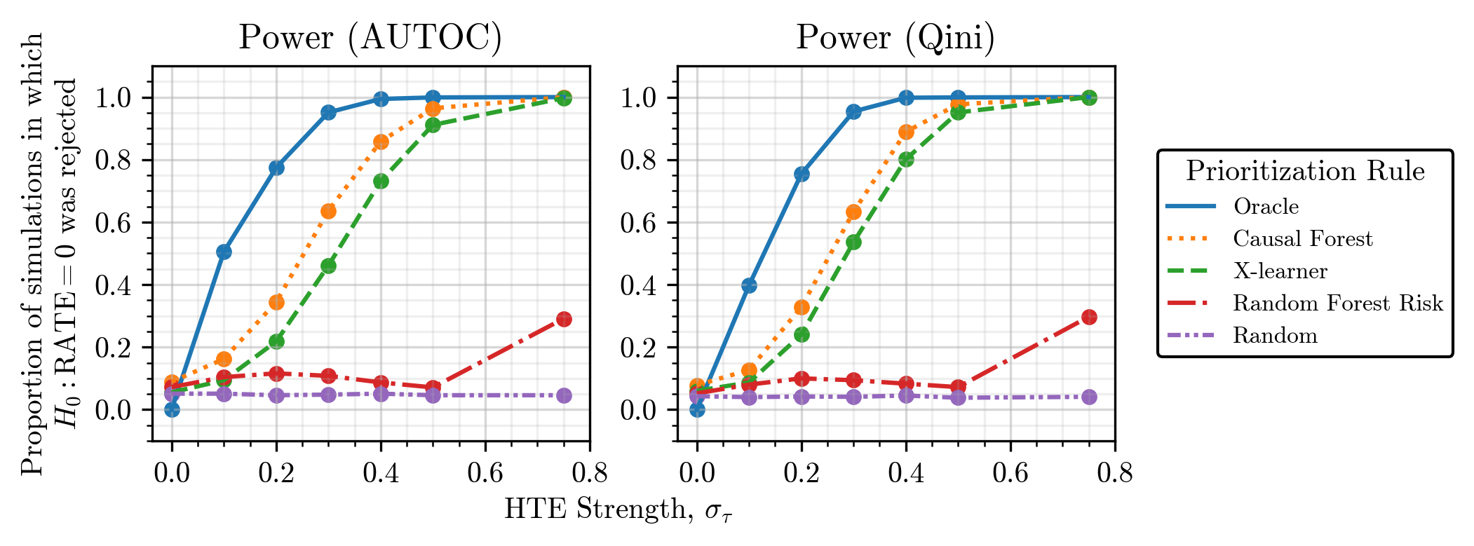
Figure 6: Power as a function of heterogeneous treatment effect strength, $\sigma_{\tau}$, in Setup 1 for the RATE with both logarithmic (AUTOC) and linear (Qini) weighting. Of note, even when $\sigma_{\tau}=0.3$ i.e. the variance/signal strength of the heterogeneous treatment effects was $\sigma_{\tau}^{2}/\sigma_{\varepsilon}^{2}=0.3^{2}=0.09\approx 10\%$ that of the noise in the observed outcome model, we were able to use the procedure outlined in Section A.4 to test against the presence of heterogeneous treatment effects with a power of $>0.6$ and a Type I error of approximately $0.05$. Once the signal-to-noise ratio approached closer to $\sigma_{\tau}^{2}/\sigma_{\varepsilon}^{2}=0.4^{2}=0.16$, we were able to test against the presence of heterogeneous treatment effects with a power of $>0.8$ and a Type I error of $0.05$ using the Causal Forest implemented in grf with default hyperparameters.

C.3.2 Power as a function of sample size

Using the simulator described in Section C.2.1, we estimated statistical power via the procedure outlined in the previous section. Here, however, instead of measuring power as a function of varying heterogeneous treatment effect strength, we analyzed how power changed with increasing sample size.

See Figure 7 for a summary of the results. Of note, the RATE increased monotonically with the sample size for prioritization rules that directly target the CATE (e.g., the Causal Survival Forest and Cox Proportional Hazards S-learner models). The same is not true of prioritization rules that only targeted risk/the baseline outcome (e.g., the Random Survival Forest Risk model).

Figure 7: Statistical power in testing against the absence of heterogeneous treatment effects, as a function of sample size (train and test set size are identical within each simulation), in the context of right-censored, time-to-event outcomes under unconfoundedness.

C.3.3 Power vs. Weighting Function

In our simulation section, “Section 4: Choosing a RATE Metric and Score”, we considered two aspects of the RATE estimator that impact its statistical power for detecting treatment effect heterogeneity: (1) the weighting function $\alpha(\cdot)$ (e.g., Qini vs. AUTOC), and (2) the form for the score, $\widehat{\Gamma}_{i}$ (e.g., AIPW vs. IPW scores).

Regarding (1), the weighting function, we showed in simulation that the AUTOC yields greater statistical power than the Qini coefficient when only a small subset of the population experiences nontrivial heterogeneous treatment effects whereas the Qini coefficient yields greater power when heterogeneous treatment effects are diffuse and substantial across the population (see Figure 2 in the main manuscript). This simulation was performed using AIPW oracle scores, $\Gamma^{*}_{i}$, as given in Equation 2.13. For these Oracle scores, we assume nuisance parameters are known a priori, including $m(x,w)$ which represents the expected outcome given a subject’s covariates, $x$, and treatment assignment, $w\in\{0,1\}$. In practice, however, one never has access to $m(x,w)$ and this must be estimated instead. We assess the robustness/sensitivity of our findings by repeating the same experiment using Oracle scores, AIPW scores with estimated $\hat{m}(x,w)$, and IPW scores. The results are shown in Figure 8 below. Notably, the trends highlighted in the manuscript regarding the impact of weighting function on statistical power are robust to choice of score.

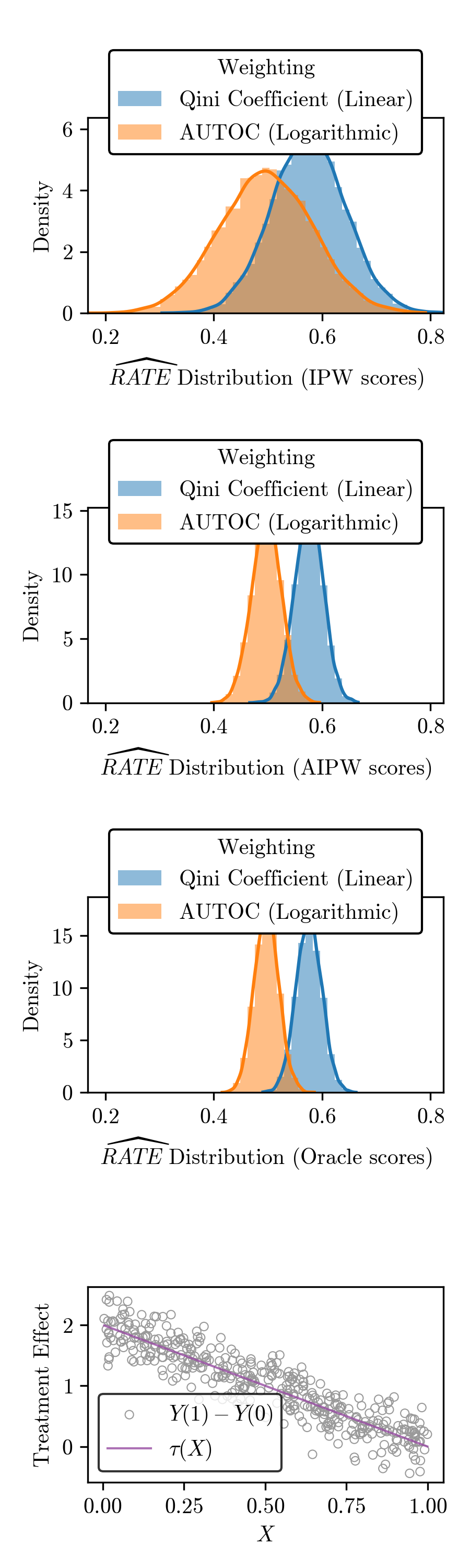
(a) 100% have $|\tau(X_{i})|>0$

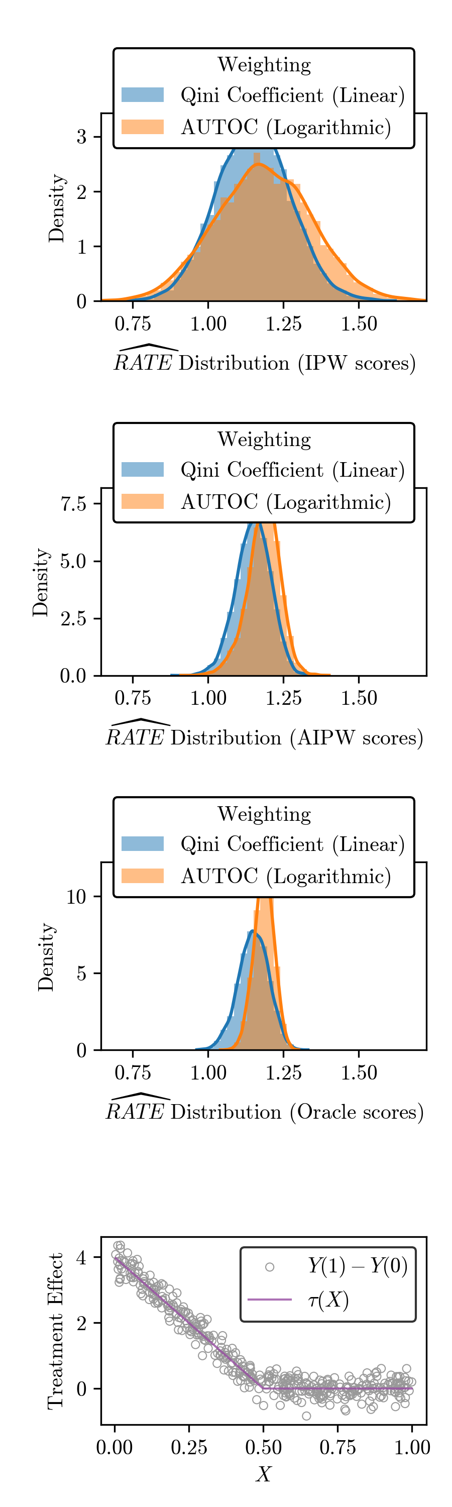
(b) 50% have $|\tau(X_{i})|>0$

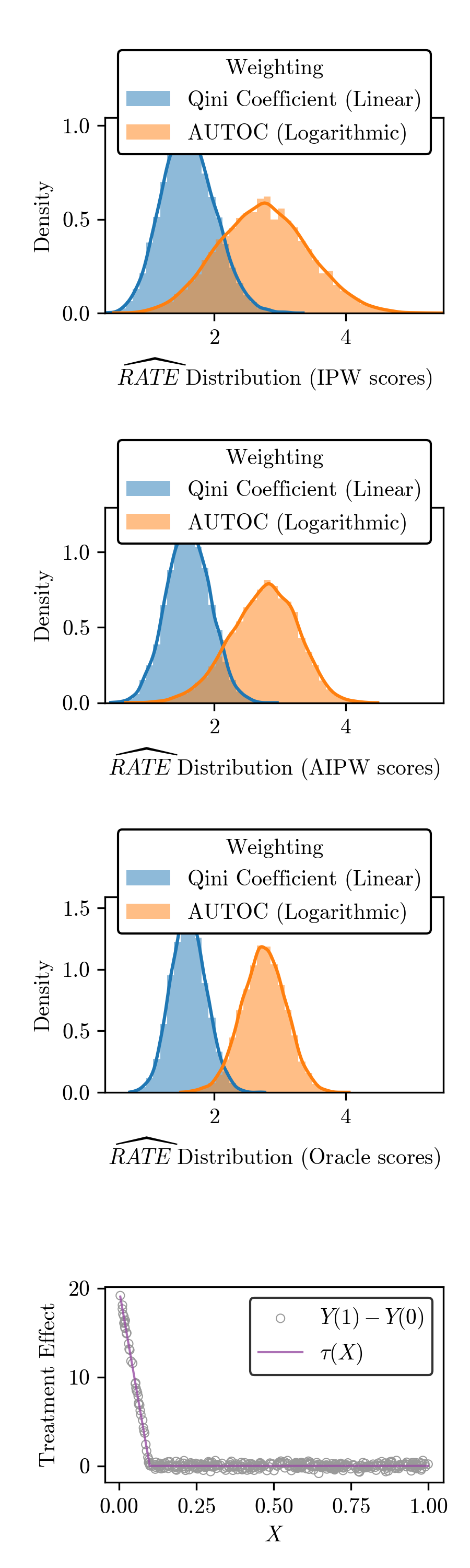
(c) 10% have $|\tau(X_{i})|>0$

Figure 8: Comparison of linear (Qini) vs. logarithmic (AUTOC) weighting functions for different scores (IPW, AIPW, and Oracle scores). If treatment effects are nonzero for a significant proportion of the population (left column) the power of the estimated RATE when using linear weighting (Qini) tends to be greater than when using logarithmic (AUTOC) weighting. Conversely, if nonzero treatment effects are concentrated among a small proportion of the population (right column) we see that using logarithmic (AUTOC) weighting leads to a greater power for the estimated RATE relative to using linear (Qini) weighting.

	ACCORD-BP		SPRINT
	n	%	n	%
Total	4684		9160
Non-Intensive	2342	50.0	4567	49.9
Intensive	2342	50.0	4593	50.1
No Diabetes	0	0.0	9160	100.0
Diabetes	4684	100.0	0	0.0
Male	2455	52.4	5908	64.5
Female	2229	47.6	3252	35.5
Non-Black	3578	76.4	6414	70.0
Black	1106	23.6	2746	30.0
Non-Hispanic	4359	93.1	8190	89.4
Hispanic	325	6.9	970	10.6
Not current smoker	4061	86.7	7932	86.6
Current smoker	623	13.3	1228	13.4
Not former smoked	2719	58.0	5265	57.5
Former smoker	1965	42.0	3895	42.5
Not on Aspirin	2225	47.5	4493	49.1
On Aspirin	2459	52.5	4667	50.9
Not on Statin	1632	34.8	5165	56.4
On Statin	3052	65.2	3995	43.6
No Angina	4153	88.7	7971	87.0
Angina	531	11.3	1189	13.0
	Mean	SD	Mean	SD
SBP	139.15	15.78	139.66	15.59
DBP	75.95	10.39	78.15	11.94
eGFR	91.57	28.78	71.80	20.60
	Median	[IQR]	Median	[IQR]
Age	62.05	[57.60, 67.10]	67.00	[61.00, 76.00]
BP medications	2.00	[1.00, 2.00]	2.00	[1.00, 3.00]
Creatinine	0.90	[0.70, 1.00]	1.01	[0.86, 1.21]
Cholesterol	188.00	[162.00, 216.25]	187.00	[161.00, 215.00]
HDL cholesterol	45.00	[37.00, 54.00]	50.00	[43.00, 60.00]
Triglycerides	147.00	[98.00, 226.25]	107.00	[77.00, 150.00]
BMI	31.63	[28.05, 35.90]	29.02	[25.88, 32.90]

Table 6: Baseline characteristics for the SPRINT and ACCORD-BP trials

Appendix D Combined analysis of SPRINT/ACCORD-BP

While in the main manuscript we train on SPRINT and evaluate on ACCORD-BP (or vice versa) to highlight how the RATE would likely be used in practice (train on one trial/population, evaluate how well prioritization rules generalize to new populations), we also recognize the value of in-distribution evaluation. In this experiment we follow the exact same protocol as described in Section 6, except that we use as our “train” set for the Causal Survival Forest, Random Survival Forest, and Cox PH S-Learner models a combined dataset generated by combining subjects from the SPRINT and ACCORD-BP trials and selecting from that set 6922 subjects (uniformly at random). The “test” is constructed in similar fashion.

Prioritization Rule	AUTOC (95% CI)	$p$-value
Causal Survival Forest (grf)	-5.83 (-14.09, 2.43)	0.17
Cox PH S-learner	-0.99 (-9.49, 7.52)	0.82
Random Survival Forest Risk (grf)	3.03 (-6.41, 12.46)	0.53
Framingham Risk Score	-7.01 (-18.89, 4.88)	0.25
ACC/AHA Pooled Cohort Equations	-1.43 (-13.22, 10.36)	0.81

Table 7: AUTOC estimates (RMST) obtained using data from a test split of a combination of both SPRINT and ACCORD-BP subjects ($n=6922$), with prioritization rules trained on SPRINT ($n=6922$), if necessary. We also show 95% confidence intervals obtained using the half-sample bootstrap, along with associated $p$-values.

References

- Andersen and Gill (1982) P. K. Andersen and R. D. Gill. Cox’s regression model for counting processes: a large sample study. The Annals of Statistics, pages 1100–1120, 1982.
- Artigao-Rodenas et al. (2013) L. M. Artigao-Rodenas, J. A. Carbayo-Herencia, J. A. Divison-Garrote, V. F. Gil-Guillen, J. Massó-Orozco, M. Simarro-Rueda, F. Molina-Escribano, C. Sanchis, L. Carrión-Valero, E. Lopez de Coca, et al. Framingham risk score for prediction of cardiovascular diseases: a population-based study from southern Europe. PloS One, 8(9):e73529, 2013.
- Ascarza (2018) E. Ascarza. Retention futility: Targeting high-risk customers might be ineffective. Journal of Marketing Research, 55(1):80–98, 2018.
- Athey and Imbens (2019) S. Athey and G. W. Imbens. Machine learning methods that economists should know about. Annual Review of Economics, 11:685–725, 2019.
- Athey and Wager (2021) S. Athey and S. Wager. Policy learning with observational data. Econometrica, 89(1):133–161, 2021.
- Athey et al. (2019) S. Athey, J. Tibshirani, and S. Wager. Generalized Random Forests. Annals of Statistics, 47(2):1148–1178, 2019.
- Basu et al. (2017) S. Basu, J. B. Sussman, and R. A. Hayward. Detecting heterogeneous treatment effects to guide personalized blood pressure treatment: a modeling study of randomized clinical trials. Annals of Internal Medicine, 166(5):354–360, 2017.
- Beddhu et al. (2018) S. Beddhu, G. M. Chertow, T. Greene, P. K. Whelton, W. T. Ambrosius, A. K. Cheung, J. Cutler, L. Fine, R. Boucher, G. Wei, et al. Effects of intensive systolic blood pressure lowering on cardiovascular events and mortality in patients with type 2 diabetes mellitus on standard glycemic control and in those without diabetes mellitus: reconciling results from ACCORD BP and SPRINT. Journal of the American Heart Association, 7(18):e009326, 2018.
- Breiman (2001) L. Breiman. Random forests. Machine learning, 45(1):5–32, 2001.
- Chen et al. (1997) Z.-M. Chen et al. CAST: randomised placebo-controlled trial of early aspirin use in 20 000 patients with acute ischaemic stroke. The Lancet, 349(9066):1641–1649, 1997.
- Chen et al. (2000) Z. Chen, P. Sandercock, H. Pan, C. Counsell, R. Collins, L. Liu, J. Xie, C. Warlow, and R. Peto. Indications for early aspirin use in acute ischemic stroke: a combined analysis of 40 000 randomized patients from the Chinese Acute Stroke Trial and the International Stroke Trial. Stroke, 31(6):1240–1249, 2000.
- Chernozhukov et al. (2018a) V. Chernozhukov, D. Chetverikov, M. Demirer, E. Duflo, C. Hansen, W. Newey, and J. Robins. Double/debiased machine learning for treatment and structural parameters. The Econometrics Journal, 21(1):C1–C68, 2018a.
- Chernozhukov et al. (2018b) V. Chernozhukov, M. Demirer, E. Duflo, and I. Fernandez-Val. Generic machine learning inference on heterogenous treatment effects in randomized experiments. Technical report, National Bureau of Economic Research, 2018b.
- Chernozhukov et al. (2022) V. Chernozhukov, J. C. Escanciano, H. Ichimura, W. K. Newey, and J. M. Robins. Locally robust semiparametric estimation. Econometrica, 90(4):1501–1535, 2022.
- Chung and Romano (2013) E. Chung and J. P. Romano. Exact and asymptotically robust permutation tests. The Annals of Statistics, 41(2):484–507, 2013.
- Cui et al. (2023) Y. Cui, M. R. Kosorok, E. Sverdrup, S. Wager, and R. Zhu. Estimating heterogeneous treatment effects with right-censored data via causal survival forests. Journal of the Royal Statistical Society Series B: Statistical Methodology, 85(2):179–211, 2023.
- D’Agostino et al. (2008) R. B. D’Agostino, R. S. Vasan, M. J. Pencina, P. A. Wolf, M. Cobain, J. M. Massaro, and W. B. Kannel. General Cardiovascular Risk Profile for Use in Primary Care. Circulation, 117(6):743–753, 2008.
- DeFilippis et al. (2015) A. P. DeFilippis, R. Young, C. J. Carrubba, J. W. McEvoy, M. J. Budoff, R. S. Blumenthal, R. A. Kronmal, R. L. McClelland, K. Nasir, and M. J. Blaha. An analysis of calibration and discrimination among multiple cardiovascular risk scores in a modern multiethnic cohort. Annals of Internal Medicine, 162(4):266–275, 2015.
- Diemert et al. (2018) E. Diemert, A. Betlei, C. Renaudin, and M.-R. Amini. A Large Scale Benchmark for Uplift Modeling. In KDD, 2018.
- Ding et al. (2016) P. Ding, A. Feller, and L. Miratrix. Randomization inference for treatment effect variation. Journal of the Royal Statistical Society: Series B: Statistical Methodology, pages 655–671, 2016.
- Dvoretzky et al. (1956) A. Dvoretzky, J. Kiefer, and J. Wolfowitz. Asymptotic Minimax Character of the Sample Distribution Function and of the Classical Multinomial Estimator. The Annals of Mathematical Statistics, 27(3):642 – 669, 1956. doi: 10.1214/aoms/1177728174. URL https://doi.org/10.1214/aoms/1177728174.
- Efron (1982) B. Efron. The jackknife, the bootstrap and other resampling plans. SIAM, 1982.
- Feigin et al. (2021) V. L. Feigin, B. A. Stark, C. O. Johnson, G. A. Roth, C. Bisignano, G. G. Abady, M. Abbasifard, M. Abbasi-Kangevari, F. Abd-Allah, V. Abedi, et al. Global, regional, and national burden of stroke and its risk factors, 1990–2019: A systematic analysis for the Global Burden of Disease Study 2019. The Lancet Neurology, 20(10):795–820, 2021.
- Fisher and Curfman (2018) N. D. Fisher and G. Curfman. Hypertension—a public health challenge of global proportions. Journal of the American Medical Association, 320(17):1757–1759, 2018.
- Friedman (1991) J. H. Friedman. Multivariate Adaptive Regression Splines. The Annals of Statistics, pages 1–67, 1991.
- Goff et al. (2014) D. C. Goff, D. M. Lloyd-Jones, G. Bennett, S. Coady, R. B. D’Agostino, R. Gibbons, P. Greenland, D. T. Lackland, D. Levy, C. J. O’Donnell, J. G. Robinson, J. S. Schwartz, S. T. Shero, S. C. Smith, P. Sorlie, N. J. Stone, and P. W. F. Wilson. 2013 ACC/AHA Guideline on the Assessment of Cardiovascular Risk. Circulation, 129(25_suppl_2):S49–S73, 2014. doi: 10.1161/01.cir.0000437741.48606.98. URL https://www.ahajournals.org/doi/abs/10.1161/01.cir.0000437741.48606.98.
- Gordon et al. (2019) B. R. Gordon, F. Zettelmeyer, N. Bhargava, and D. Chapsky. A comparison of approaches to advertising measurement: Evidence from big field experiments at Facebook. Marketing Science, 38(2):193–225, 2019.
- Green et al. (1966) D. M. Green, J. A. Swets, et al. Signal Detection Theory and Psychophysics, volume 1. Wiley New York, 1966.
- Group (2010) A. S. Group. Effects of intensive blood-pressure control in type 2 diabetes mellitus. New England Journal of Medicine, 362(17):1575–1585, 2010.
- Group (1997) I. S. T. C. Group. The International Stroke Trial (IST): a randomised trial of aspirin, subcutaneous heparin, both, or neither among 19 435 patients with acute ischaemic stroke. The Lancet, 349(9065):1569–1581, 1997.
- Group (2015) S. R. Group. A randomized trial of intensive versus standard blood-pressure control. New England Journal of Medicine, 373(22):2103–2116, 2015.
- Hastie et al. (2009) T. Hastie, R. Tibshirani, and J. Friedman. The Elements of Statistical Learning: Data Mining, Inference, and Prediction. Springer Science & Business Media, 2009.
- Hill (2011) J. L. Hill. Bayesian nonparametric modeling for causal inference. Journal of Computational and Graphical Statistics, 20(1):217–240, 2011.
- Hohnhold et al. (2015) H. Hohnhold, D. O’Brien, and D. Tang. Focus on the Long-Term: It’s better for Users and Business. In Proceedings 21st Conference on Knowledge Discovery and Data Mining, Sydney, Australia, 2015. URL http://dl.acm.org/citation.cfm?doid=2783258.2788583.
- Imai and Li (2023) K. Imai and M. L. Li. Experimental evaluation of individualized treatment rules. Journal of the American Statistical Association, 118(541):242–256, 2023.
- Imbens and Rubin (2015) G. W. Imbens and D. B. Rubin. Causal inference in statistics, social, and biomedical sciences. Cambridge University Press, 2015.
- Ishwaran et al. (2008) H. Ishwaran, U. B. Kogalur, E. H. Blackstone, M. S. Lauer, et al. Random survival forests. Annals of Applied Statistics, 2(3):841–860, 2008.
- Johnson et al. (2017) G. A. Johnson, R. A. Lewis, and E. I. Nubbemeyer. Ghost Ads: Improving the Economics of Measuring Online Ad Effectiveness. Journal of Marketing Research, 54(6):867–884, 2017.
- Kaul (2017) S. Kaul. A tale of two trials: reconciling differences in results by exploring heterogeneous treatment effects. Annals of Internal Medicine, 166(5):370–372, 2017.
- Kennedy (2023) E. H. Kennedy. Towards optimal doubly robust estimation of heterogeneous causal effects. Electronic Journal of Statistics, 17(2):3008–3049, 2023.
- Kent et al. (2016) D. M. Kent, J. Nelson, I. J. Dahabreh, P. M. Rothwell, D. G. Altman, and R. A. Hayward. Risk and treatment effect heterogeneity: re-analysis of individual participant data from 32 large clinical trials. International journal of epidemiology, 45(6):2075–2088, 2016.
- Kent et al. (2020) D. M. Kent, D. van Klaveren, J. K. Paulus, R. D’Agostino, S. Goodman, R. Hayward, J. P. Ioannidis, B. Patrick-Lake, S. Morton, M. Pencina, G. Raman, J. S. Ross, H. P. Selker, R. Varadhan, A. Vickers, J. B. Wong, and E. W. Steyerberg. The Predictive Approaches to Treatment effect Heterogeneity (PATH) Statement. Annals of Internal Medicine, 172(1):35–45, 2020.
- Künzel et al. (2019) S. R. Künzel, J. S. Sekhon, P. J. Bickel, and B. Yu. Metalearners for estimating heterogeneous treatment effects using machine learning. Proceedings of the National Academy of Sciences, 116(10):4156–4165, 2019.
- Mammen (2012) E. Mammen. When does bootstrap work?: Asymptotic results and simulations, volume 77. Springer Science & Business Media, 2012.
- Manski (2004) C. F. Manski. Statistical treatment rules for heterogeneous populations. Econometrica, 72(4):1221–1246, 2004.
- Muntner et al. (2018) P. Muntner, R. M. Carey, S. Gidding, D. W. Jones, S. J. Taler, J. T. Wright Jr, and P. K. Whelton. Potential US population impact of the 2017 ACC/AHA high blood pressure guideline. Circulation, 137(2):109–118, 2018.
- Nie and Wager (2021) X. Nie and S. Wager. Quasi-oracle estimation of heterogeneous treatment effects. Biometrika, 108(2):299–319, 2021.
- Oikonomou et al. (2022) E. K. Oikonomou, E. S. Spatz, M. A. Suchard, and R. Khera. Individualising intensive systolic blood pressure reduction in hypertension using computational trial phenomaps and machine learning: a post-hoc analysis of randomised clinical trials. The Lancet Digital Health, 4(11):e796–e805, 2022.
- Owolabi et al. (2021) M. O. Owolabi, A. G. Thrift, A. Mahal, M. Ishida, S. Martins, W. D. Johnson, J. Pandian, F. Abd-Allah, J. Yaria, H. T. Phan, et al. Primary stroke prevention worldwide: translating evidence into action. The Lancet Public Health, 2021.
- Powers et al. (2019) W. J. Powers, A. A. Rabinstein, T. Ackerson, O. M. Adeoye, N. C. Bambakidis, K. Becker, J. Biller, M. Brown, B. M. Demaerschalk, B. Hoh, et al. Guidelines for the early management of patients with acute ischemic stroke: 2019 update to the 2018 guidelines for the early management of acute ischemic stroke: a guideline for healthcare professionals from the American Heart Association/American Stroke Association. Stroke, 50(12):e344–e418, 2019.
- Præstgaard and Wellner (1993) J. Præstgaard and J. A. Wellner. Exchangeably weighted bootstraps of the general empirical process. The Annals of Probability, pages 2053–2086, 1993.
- Psaty et al. (2003) B. M. Psaty, T. Lumley, C. D. Furberg, G. Schellenbaum, M. Pahor, M. H. Alderman, and N. S. Weiss. Health outcomes associated with various antihypertensive therapies used as first-line agents: a network meta-analysis. Journal of the American Medical Association, 289(19):2534–2544, 2003.
- Radcliffe and Surry (1999) N. Radcliffe and P. Surry. Differential response analysis: Modeling true responses by isolating the effect of a single action. Credit Scoring and Credit Control IV, 1999.
- Radcliffe (2007) N. J. Radcliffe. Using control groups to target on predicted lift: Building and assessing uplift models. Direct Marketing Analytics Journal, 1(3):14–21, 2007.
- Rekkas et al. (2020) A. Rekkas, J. K. Paulus, G. Raman, J. B. Wong, E. W. Steyerberg, P. R. Rijnbeek, D. M. Kent, and D. van Klaveren. Predictive approaches to heterogeneous treatment effects: a scoping review. BMC Medical Research Methodology, 20(1):1–12, 2020.
- Robins et al. (1994) J. M. Robins, A. Rotnitzky, and L. P. Zhao. Estimation of regression coefficients when some regressors are not always observed. Journal of the American statistical Association, 89(427):846–866, 1994.
- Rosenbaum and Rubin (1983) P. R. Rosenbaum and D. B. Rubin. The central role of the propensity score in observational studies for causal effects. Biometrika, 70(1):41–55, 1983.
- Sandercock et al. (2011) P. A. Sandercock, M. Niewada, and A. Członkowska. The international stroke trial database. Trials, 12(1):1–7, 2011.
- Saposnik et al. (2008) G. Saposnik, R. Cote, S. Phillips, G. Gubitz, N. Bayer, J. Minuk, and S. Black. Stroke outcome in those over 80: a multicenter cohort study across Canada. Stroke, 39(8):2310–2317, 2008.
- Semenova and Chernozhukov (2021) V. Semenova and V. Chernozhukov. Debiased machine learning of conditional average treatment effects and other causal functions. The Econometrics Journal, 24(2):264–289, 2021.
- Shorack (1972) G. R. Shorack. Functions of order statistics. The Annals of Mathematical Statistics, 43(2):412–427, 1972.
- Shorack and Wellner (2009) G. R. Shorack and J. A. Wellner. Empirical Processes with Applications to Statistics. SIAM, 2009.
- Sun et al. (2021) H. Sun, S. Du, and S. Wager. Treatment Allocation under Uncertain Costs. arXiv preprint arXiv:2103.11066, 2021.
- Therneau and Grambsch (2000) T. M. Therneau and P. M. Grambsch. The Cox model. In Modeling Survival Data: Extending the Cox Model, pages 39–77. Springer, 2000.
- Tsiatis (2007) A. Tsiatis. Semiparametric theory and missing data. Springer Science & Business Media, 2007.
- Ullberg et al. (2015) T. Ullberg, E. Zia, J. Petersson, and B. Norrving. Changes in functional outcome over the first year after stroke: an observational study from the Swedish stroke register. Stroke, 46(2):389–394, 2015.
- Van Der Vaart and Wellner (1996) A. W. Van Der Vaart and J. A. Wellner. Weak Convergence. In Weak Convergence and Empirical Processes, pages 16–28. Springer, 1996.
- Wager and Athey (2018) S. Wager and S. Athey. Estimation and inference of heterogeneous treatment effects using random forests. Journal of the American Statistical Association, 113(523):1228–1242, 2018.
- Whelton et al. (2018) P. K. Whelton, R. M. Carey, W. S. Aronow, D. E. Casey, K. J. Collins, C. Dennison Himmelfarb, S. M. DePalma, S. Gidding, K. A. Jamerson, D. W. Jones, et al. 2017 ACC/AHA/AAPA/ABC/ACPM/AGS/APhA/ASH/ASPC/NMA/PCNA guideline for the prevention, detection, evaluation, and management of high blood pressure in adults: a report of the American College of Cardiology/American Heart Association Task Force on Clinical Practice Guidelines. Journal of the American College of Cardiology, 71(19):e127–e248, 2018.
- Xu et al. (2023) Y. Xu, N. Ignatiadis, E. Sverdrup, S. Fleming, S. Wager, and N. Shah. Treatment heterogeneity with survival outcomes. In Handbook of Matching and Weighting Adjustments for Causal Inference, pages 445–482. Chapman and Hall/CRC, 2023.
- Yadlowsky et al. (2018) S. Yadlowsky, R. A. Hayward, J. B. Sussman, R. L. McClelland, Y.-I. Min, and S. Basu. Clinical implications of revised pooled cohort equations for estimating atherosclerotic cardiovascular disease risk. Annals of Internal Medicine, 169(1):20–29, 2018.
- Zhao et al. (2013) L. Zhao, L. Tian, T. Cai, B. Claggett, and L.-J. Wei. Effectively selecting a target population for a future comparative study. Journal of the American Statistical Association, 108(502):527–539, 2013.
- Zheng and van der Laan (2011) W. Zheng and M. J. van der Laan. Cross-validated targeted minimum-loss-based estimation. In Targeted Learning, pages 459–474. Springer, 2011.
- Zweig and Campbell (1993) M. H. Zweig and G. Campbell. Receiver-operating characteristic (ROC) plots: a fundamental evaluation tool in clinical medicine. Clinical Chemistry, 39(4):561–577, 1993.
- van der Vaart (1998) A. W. van der Vaart. Asymptotic Statistics. Cambridge Series in Statistical and Probabilistic Mathematics. Cambridge University Press, 1998.