Big bang as a topological quantum phase transition

Abstract

It has been argued that a particular type of quantum-vacuum variable $q$ can provide a solution to the main cosmological constant problem and possibly also give a cold-dark-matter component. We now show that the same $q$-field may suggest a new interpretation of the big bang, namely as a quantum phase transition between topologically inequivalent vacua. These two vacua are characterized by the equilibrium values $q=\pm\,q_{0}$ and there is a kink-type solution $q(t)$ interpolating between $q=-q_{0}$ for $t\to-\infty$ and $q=+q_{0}$ for $t\to\infty$, with conformal symmetry for $q=0$ at $t=0$.

I Introduction

Several years ago, we have proposed a condensed-matter-inspired approach to the cosmological constant problem Weinberg1988 . Our approach goes under the name of $q$-theory KlinkhamerVolovik2008a ; KlinkhamerVolovik2008b ; KlinkhamerVolovik2009 ; KlinkhamerVolovik2016-CCP ; KlinkhamerVolovik2016-brane and we present a brief review in App. A. This “$q$” is a microscopic (high-energy) variable of the quantum vacuum and its macroscopic (low-energy) equations are Lorenz invariant and governed by thermodynamics. Later, we have also realized that rapid oscillations of the $q$-field can act as a cold-dark-matter component KlinkhamerVolovik2016-q-DM ; KlinkhamerVolovik2016-more-q-DM ; KlinkhamerMistele2017 ; NittaYokokura2019 .

Now, we will discuss a third possible application of the $q$-field, namely as an effective regulator of the big bang singularity. As $q$ is the variable that describes the deep quantum vacuum, all coupling constants of the Standard Model, as well as the gravitational coupling constant $G$, are functions of $q$. An appropriate functional dependence $G(q)$ may actually lead to a kink-type behavior $q(t)$ of the vacuum variable and a corresponding bounce-type behavior of the cosmic scale factor $a(t)$. Our scenario replaces the big bang singularity HawkingEllis1973 of the Friedmann cosmology by a topological quantum phase transition (see, e.g., Refs. QPT-review1 ; QPT-review2 ; QPT-review3 ; QPT-review4 for four complementary reviews on the physics of quantum phase transitions).

Topological matter HasanKane2010 ; Wieder-etal2021 and the topological quantum vacuum are characterized by topological quantum numbers, such as the Chern number, which is typically an integer. For a continuous variation of the parameters of the system, the topological vacuum can experience a topological quantum phase transition with a change in the value of the topological invariant. As an integer invariant cannot vary continuously, the intermediate state of a topological transition may have special properties. For example, if a discrete or continuous symmetry is broken in the vacua on both sides of the transition, then this symmetry can be restored in the intermediate state. In particular, if the transition takes place between two fully gapped (massive) vacua, then the intermediate state is gapless (massless) QPT-review4 . In our scenario, the “big bang” represents such a specific intermediate state between two vacua with nontrivial topology. Here, the intermediate state is the trivial vacuum in which gravity is absent (i.e., $1/G=0$, so that there is no Einstein–Hilbert term in the action) and the conformal symmetry is restored.

In this reinterpretation of the “big bang,” the metric is kept unchanged in the standard Robertson–Walker form (unlike the different metric used in Refs. Klinkhamer2019 ; Klinkhamer2019-More ; KlinkhamerWang2019 ; KlinkhamerWang2020 ; see Ref. Klinkhamer2021-APPB-review for a review which also contains the original references of Friedmann and others). In fact, the result of the present paper improves upon an earlier kink-bounce solution Klinkhamer2020-Another , which had a completely ad hoc underlying theory. Here, the underlying theory has a direct physical motivation, as will become clear in the following.

II Anomaly-type term

The standard topological $\Theta$ term in the action has the following form:

$$S_{\Theta}=-\frac{1}{4\pi}\,\epsilon^{\alpha\beta\gamma\delta}\int d^{4}x\,\Theta\,F_{\alpha\beta}F_{\gamma\delta}\,.$$ (1)

Here, there is a 2-form curvature $F=dA$ from a 1-form gauge field $A$. Natural units with $\hbar=c=1$ are used throughout. In topological vacua, such as topological insulators HasanKane2010 , $\Theta$ is determined by a (quantized) topological invariant. This topological invariant is, in fact, given by the second Chern number expressed in terms of the Green’s functions as an integral over the Brillouin zone of the crystalline topological insulator; see, e.g., Ref. NissinenVolovik2019 .

The topological vacuum may also contain higher-form gauge fields Gaiotto-etal2015 ; Dubinkin2020 . In the present paper, we focus on a 3-form gauge field 3-form-A-first-batch ; 3-form-A-second-batch ; 3-form-A-third-batch , for which the topological term reads Gaiotto-etal2015

$$S_{\phi}=-\frac{1}{2\pi}\int\phi\,dA^{(3)}\,,$$ (2)

with a dimensionless (pseudo)scalar field $\phi$ [here, and in the following, we put “pseudo” in parentheses, as we do not know the microscopic origin of the 3-form gauge field and its transformation properties]. The main reason for considering topological vacua with a 3-form gauge field is that, as emphasized by Hawking 3-form-A-second-batch , in particular, the 3-form gauge field can perhaps solve the cosmological constant problem.

In our approach KlinkhamerVolovik2008a ; KlinkhamerVolovik2008b , the parameter $\Theta$ or $\phi$ plays the role of a dimensionless chemical potential $\mu$ and (2) becomes

$$S_{\mu}=-\frac{1}{24}\,\epsilon^{\alpha\beta\gamma\delta}\int d^{4}x\,\mu\,F_{\alpha\beta\gamma\delta}\,.$$ (3)

Using the proper normalization of the 3-form, we can choose $\mu=\pm 1$. In principle, we may consider $\Theta$ and $\mu$ as a dimensionless (pseudo)scalar field $\chi$ with periodicity $\chi=\chi+2\pi$. But, here, we consider this (pseudo)scalar $\mu$ as a constant, because it is the constant of motion of the dynamics. Simultaneously, $\mu$ may serve as a topological invariant, which changes abruptly in the topological quantum phase transition across the “big bang.”

III Vacuum variable

The vacuum variable $q$ can be written in terms of the 4-form field strength by the following expression:

$$F_{\alpha\beta\gamma\delta}=q\,e\,\epsilon_{\alpha\beta\gamma\delta}\,,$$ (4)

where $e$ is the tetrad determinant and $\epsilon_{\alpha\beta\gamma\delta}$ the completely antisymmetric Levi–Civita symbol normalized to unity. The (pseudo)scalar $q$ has a mass dimension of 4, while $\mu$ is dimensionless. Remark that this vacuum variable $q$ differs from the one used in our previous papers KlinkhamerVolovik2008b ; KlinkhamerVolovik2016-CCP and App. A.3 here, where the vacuum variable has a mass dimension of 2.

The term (3) now has the form

$$S_{\mu}=-\int d^{4}x\,e\,\mu\,q\,.$$ (5)

Precisely this term $-\mu\,q$ enters the Einstein gravitational equation and cancels the vacuum energy density $\epsilon(q)$ in equilibrium for $q=q_{0}$, where $[d\epsilon/dq\,]_{q=q_{0}}=\mu$. The thermodynamic (macroscopic) vacuum energy,

$$\rho_{V}(q)\equiv\epsilon(q)-\mu\,q\,,$$ (6)

enters the Einstein equation as a cosmological-constant term and self-adjusts to zero in equilibrium KlinkhamerVolovik2008a . For the record, this Einstein equation is given by (26) in App. A.3, where $q$ is denoted $F$.

Starting from the definition (6), we recall the equilibrium conditions KlinkhamerVolovik2008a :

$$\rho_{V}(q_{0}) = 0\,,$$ (7a)

$$\rho_{V}^{\prime}(q_{0}) = 0\,,$$ (7b)

$$\rho_{V}^{\prime\prime}(q_{0}) > 0\,,$$ (7c)

where the prime stands for differentiation with respect to $q$. Note that (7b) fixes $\mu$ to the equilibrium value

$$\mu_{0}\equiv\left.\frac{\epsilon(q)}{dq}\right|_{q=q_{0}}\,.$$ (8)

It remains an outstanding task to find a proper microscopic realization of $q$-theory that produces the vacuum energy density $\epsilon(q)$ and the corresponding equilibrium values $q_{0}$ and $\mu_{0}$, possibly with $\mu_{0}$ appearing as a (quantized) topological invariant.

IV Quantum phase transition

IV.1 Setup

If $\mu$ is a type of topological invariant, then $1/G$ should play the same role as the gap in the spectrum of a topological insulator: $\mu$ becomes zero at the transition between distinct topological vacua. Conformal symmetry is restored at the transition point. In this approach, the “big bang” would be represented as a topological quantum phase transition from the $\mu=+1$ equilibrium state to the $\mu=-1$ equilibrium state via the trivial vacuum state with $q=0$ (and $\mu=0$).

In the trivial vacuum, both gravity and vacuum energy are absent, and this vacuum obeys conformal symmetry. In view of the mass dimension 4 of the $q$ variable and the proper normalization of Newton’s “constant,” the natural choice for the dependence of $1/G$ on $q$, which is consistent with conformal symmetry, is as follows:

$$\frac{1}{G(q)}=\sqrt{|q|}\,.$$ (9)

It appears impossible to obtain an analytic $q$ behavior of $1/G(q)$ without use of an energy scale $q_{0}>0$, an example being $1/G(q)=q^{2}/(q_{0})^{3/2}$. We prefer the Ansatz (9), which is consistent with having conformal symmetry at $q=0$.

For our cosmological discussion, we take the standard spatially flat Robertson–Walker metric HawkingEllis1973 ,

$$ds^{2} \equiv g_{\alpha\beta}(x)\,dx^{\alpha}\,dx^{\beta}=-dt^{2}+a^{2}(t)\;\delta_{ab}\,dx^{a}\,dx^{b}\,,$$ (10a)

$$a(t) \in \mathbb{R}\,,$$ (10b)

$$t \in (-\infty,\,\infty)\,,\quad x^{a}\in(-\infty,\,\infty)\,,$$ (10c)

where $t$ is the cosmic time coordinate given by $x^{0}=t$ and $a(t)$ the cosmic scale factor. The spatial indices $a$, $b$ in (10a) run over $\{1,\,2,\,3\}$. The generalized Maxwell equation for the 4-form field strength and the generalized Einstein equation then give the following equations for $q(t)$ and the Hubble parameter $H(t)\equiv[da(t)/dt]/a(t)$:

$$\frac{d\rho_{V}}{dq} = \frac{d(G^{-1})}{dq}\left(\frac{dH}{dt}+2\,H^{2}\right)\,,$$ (11a)

$$\rho_{V} = G^{-1}\,H^{2}+H\,\frac{d(G^{-1})}{dt}\,,$$ (11b)

where the vacuum energy density $\rho_{V}(q)$ has been defined in (6). The above equations appear as (30) and (31a) in App. A.3, for $\rho_{M}=P_{M}=0$ [in these equations, $q$ is denoted by $F$ and the factor $8\pi/3$ there will be absorbed into $G(q)$ here]. It needs to be emphasized that the original expressions (25) and (26) in App. A.3 are

universal KlinkhamerVolovik2008a ; KlinkhamerVolovik2008b , that is, independent of the particular realization of the conserved variable $q$.

For a constant gravitational coupling, $G(q)=(8\pi/3)\,G_{N}$, (11a) forces the vacuum energy density to be a constant (assumed to be nonnegative), $\rho_{V}(q)=\text{const}=\Lambda\geq 0$. In addition, (11b) reduces to the standard Friedmann equation, $H^{2}=(8\pi/3)\,G_{N}\,\Lambda$, with a cosmological constant $\Lambda$ and no matter. Equation (11b) makes clear that having a nonconstant gravitational coupling $G(q)$ significantly modifies the structure of the Friedmann equation. This observation contrasts with what happens for the “regularized” metric of Refs. Klinkhamer2019 ; Klinkhamer2019-More , which only changes the $H^{2}$ term of the Friedmann equation by a multiplicative Jacobian term, as shown by Eq. (3.3a) of Ref. Klinkhamer2019 .

IV.2 Vacuum energy

The general behaviour of a self-sustained vacuum does not depend much on the particular choice of the vacuum energy density $\epsilon(q)$ in the action. There are only the following requirements: $\epsilon(q)$ should be zero in the trivial vacuum ($q=0$) and the trivial vacuum should be unstable towards the equilibrium vacuum ($q=q_{0}\neq 0$). The simplest possible form is

$$\frac{\epsilon(q)}{q_{0}}=-\frac{3}{2}\,\frac{q^{2}}{q_{0}^{2}}+\frac{1}{2}\,\frac{q^{4}}{q_{0}^{4}}\,.$$ (12)

Here, $q_{0}>0$ is the magnitude of $q$ in equilibrium, so that the present Newton “constant” is given by $G_{N}=3/(8\pi)\,G(q_{0})$. We have also used a particular normalization, so that the equilibrium vacua have chemical potentials $\mu=\pm 1$, which are assumed to correspond to topological quantum numbers of the vacuum. The value of the chemical potential in the equilibrium vacuum fully determines the coefficients $-3/2$ and $1/2$ in (12).

Note that the trivial vacuum with $q=1/G=0$ and the real vacuum with $q=\pm q_{0}$ have the same thermodynamic vacuum energy: $\rho_{V}(0)=\rho_{V}(q_{0})$. This agrees with the multiple-point criticality principle FroggattNielsen1996 ; Sidharth2016 ; Volovik2004 . However, as distinct from the multiple-point criticality principle, one of these vacua is unstable. Actually, we can also use another form of $\epsilon(q)$, in which both vacua are locally stable. In quantum liquids, our construction corresponds to the coexistence of liquid and vapour at a nonzero pressure, while at zero pressure the gas phase is unstable towards the liquid phase.

Figure 1 shows, for later reference, the vacuum energy density $\rho_{V}(q)$ from (6) and (12) at three different values of the chemical potential $\mu$ [the middle panel shows, in fact, the Ansatz function $\epsilon(q)$]

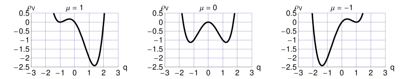
Figure 1: Vacuum energy density $\rho_{V}(q)$ from (6) for three different values of the chemical potential, $\mu=1,\,0,\,-1$. The $\epsilon(q)$ Ansatz (12) has been used and the scale $q_{0}$ has been set to unity. According to (7), the stable equilibrium value of the vacuum variable is $q=-q_{0}=-1$ for chemical potential $\mu=1$ and $q=q_{0}=1$ for $\mu=-1$. For chemical potential $\mu=0$, the equilibrium state $q=0$ is unstable. The left panel refers to one phase of the quantum vacuum (characterized by $\mu=1$) and the right panel to another phase (characterized by $\mu=-1$).

IV.3 Modified big bang

Let us, first, find a solution at small $|t|\ll t_{0}\sim q_{0}^{-1/4}$, i.e., for times shorter than the Planck time. From (11) and (12), we obtain for small positive $t$:

$$q = q_{0}\;\frac{t^{2}}{t_{0}^{2}}\,\,,\,\,H=q_{0}^{1/2}\;\frac{t^{2}}{t_{0}}\,\,,\,\,G^{-1}=q_{0}^{1/2}\;\frac{t}{t_{0}}\,,$$ (13a)

$$\mu = -1\,.$$ (13b)

For later times, $t\gg t_{0}$, the solution will have oscillations KlinkhamerVolovik2008b , which asymptotically approach the Minkowski vacuum with $|q|=q_{0}$.

There are now two possible extensions to negative $t$. The first extension is symmetric with respect to time reversal,

$$q = q_{0}\;\frac{t^{2}}{t_{0}^{2}}\,\,,\,\,H=q_{0}^{1/2}\;\frac{t^{2}}{t_{0}}\,\,,\,\,G^{-1}=q_{0}^{1/2}\;\frac{|t|}{t_{0}}\,,$$ (14a)

$$\mu = -1\,,$$ (14b)

and the second extension antisymmetric (see App. B for further details),

$$q = q_{0}\;\frac{t\,|t|}{t_{0}^{2}}\,\,,\,\,H=q_{0}^{1/2}\;\frac{t\,|t|}{t_{0}}\,\,,\,\,G^{-1}=q_{0}^{1/2}\;\frac{|t|}{t_{0}}\,,$$ (15a)

$$\mu = -\mathrm{sgn}\,t\,.$$ (15b)

The symmetric case (14) does not have topological stability, since the “big bang” connects two topologically equivalent vacua (each having $\mu=-1$). The antisymmetric case (15), on the other hand, has the “big bang” (or, more precisely, the “bounce”) serving as a boundary between different topological vacua (going, in Fig. 1, from the left panel, via the middle panel, to the right panel), and this boundary corresponds to the gapless boundary state of topological insulators.

In our case, the role of the gap is played by the quantities $q$, $\mu$, $1/G$, $\epsilon$, and $\rho_{V}$, which are all nullified in this boundary state. Remark that this behavior of $1/G$, in particular, is the opposite from that of an earlier kink-bounce solution Klinkhamer2020-Another , which had $G_{\text{eff}}\sim t^{2}$, whereas here it is $1/G$ that vanishes at $t=0$, as well as all energy densities.

IV.4 Possible physical interpretation

We have presented further analytic and numeric results in App. B. These results give the behavior for a cosmic time $t$ running over the whole real axis, with an even solution $a(t)\geq 1$ having $a(t)\to\infty$ for $t\to\pm\infty$ and $a(0)=1$. The interpretation of this complete solution is, however, rather subtle. The crucial point is to realize that $t$ (or its dimensionless counterpart $\tau$) is merely a time coordinate and not a “physical” time. The “thermodynamic” time $\mathcal{T}$ (pressureless matter perturbations growing with increasing values of $\mathcal{T}$) is, most likely, given by $|t|$. If we call the $t>0$ universe $U$ and the $t<0$ universe $\overline{U}$, then the solution of App. B corresponds to two universes (or possibly a universe-antiuniverse pair) with local thermodynamic times:

$$\mathcal{T}_{\,U} = t\,,\phantom{-}\;\;\text{for}\;\;t>0\,,$$ (16a)

$$\mathcal{T}_{\,\overline{U}} = -t\,,\;\;\text{for}\;\;t<0\,.$$ (16b)

A brief discussion of the “thermodynamic” time is given in the last paragraph of Sec. IV of Ref. KlinkhamerWang2020 and a brief discussion of the two-universes interpretation in the second point of Sec. 3.2 of Ref. Klinkhamer2021-APPB-review . The scenario of a universe-antiuniverse pair was first considered in Ref. BoyleFinnTurok2018 , with a follow-up paper in Ref. BoyleTurok2021a . The strict validity of the papers BoyleFinnTurok2018 ; BoyleTurok2021a is, however, rather doubtful, as the Einstein gravitational equation used may not hold for an infinite matter energy density and an infinite Kretschmann curvature scalar Klinkhamer2019 .

So, the physical picture we have is as follows. The “big bang” is replaced by a topological quantum phase transition in the vacuum, which corresponds to a “temporal” kink-type solution of the vacuum variable $q(t)$. (Recall that the standard kink solution has the scalar field changing in a spacelike direction.) The center of the kink-type solution requires the strict absence of matter. Matter may be generated by the oscillations of the vacuum variable $q$ as discussed in App. B. It may, however, be that the proper physical interpretation of the solution obtained in App. B is not that of a bouncing cosmology (starting from $t=-\infty$, passing through a bounce at $t=0$, and proceeding on to $t=\infty$), but rather that of a creation process at $t=0$, with two more or less equivalent branches: $U$ for $t>0$ and $\overline{U}$ for $t<0$.

V Outlook

The question arises as to the origin of the 3-form gauge field, which appears to be essential for a proper description of the quantum vacuum. One possible answer to this question may come from the discussion in Ref. BoyleTurok2021b . It is shown there that, in order to cancel all quantum anomalies, we may need, in addition to the fundamental fermionic and gauge fields, also certain scalars with mass dimension zero. Our chemical potential $\mu$ is conjugate to the 4-form field strength $F$ (as discussed in Secs. II and III) and may be an example of such a dimensionless field. Recall that the (pseudo)scalar $q$ follows from the 4-form field strength $F$ by the expression (4).

On the other hand, if the “big bang” is regular, i.e., fully determined by the dynamics of $q$ and the metric, then the chemical potential is a dynamical invariant of these equations and thus cannot change sign in this regular “big bang.” Then it would make sense to consider the “big bang” with an antisymmetric tetrad determinant, $e(t)=-e(-t)$, as discussed in Refs. BoyleFinnTurok2018 ; BoyleTurok2021a ; Volovik2019 . In this case, $q(t)$ can change sign with a fixed value of the chemical potential. However, this scenario would require an extra equation for $e(t)$. For that reason, it would seem preferable to use a theory in which $e(t)$ is the order parameter of the symmetry breaking phase transition, so that $e(t)$ would play the role of the vacuum variable (cf. Refs. KlinkhamerVolovik2019 ; Zubkov2019 ; KlinkhamerVolovik2021-in-preparation ).

In the discussion of the previous paragraph, we have implicitly considered the evolution from $t=-\infty$ to $t=+\infty$ (or vice versa), but it is also possible that a universe-antiuniverse pair “starts” at $t=0$, as discussed in Sec. IV.4 and perhaps in line with remark (ii) in the last section of Ref. BoyleTurok2021a . There is then a creation process at the coordinate value $t=0$, which gives rise to a universe $U$ with chemical potential $\mu=-1$ (for an appropriate normalization) and an antiuniverse $\overline{U}$ with chemical potential $\mu=1$. In fact, there would be an emergent spacetime at $t=0$ with the proper matter fields and constants relevant to both branches $U$ and $\overline{U}$, which each would have a thermodynamic time $\mathcal{T}$ as given by (16a) and (16b), respectively.

One possible origin for such an emergent spacetime (both its points and its metric) would be the IIB matrix model IKKT-1997 ; Aoki-etal-review-1999 ; Klinkhamer2021-master , with further references in the review Klinkhamer2021-APPB-review . The interest of the IIB matrix model is that it appears to provide an “existence proof” for the idea of emergent spacetime and matter, but what new physics really replaces Friedmann’s big bang singularity remains an open question. Perhaps the main result of the present paper provides a clue, namely that we have obtained a kink-type solution $q(t)$ of the vacuum variable with a vanishing Hubble parameter $H$ precisely at the central point of the kink-type solution with $q=0$ and conformal symmetry.

Appendix A Background material

In this appendix, we provide some background on a particular condensed-matter-physics approach ($q$-theory) to the cosmological constant problem (CCP).

A.1 CCP from the condensed-matter point of view

In condensed matter physics, we know both the infrared (IR) low-energy limit described by the effective quantum fields and the ultraviolet (UV) high-energy limit corresponding to the atomic physics, the analog of Planck-scale quantum gravity. That is why we can explicitly see how the zero-point energy of the effective quantum fields in the IR are completely canceled by the UV degrees of freedom in the ground state of any condensed matter system. This occurs due the general thermodynamic Gibbs–Duhem relation, which is applicable to any system, be it the relativistic quantum vacuum of elementary particle physics or the nonrelativistic equilibrium states of condensed matter physics. Such a natural cancellation of the vacuum energy in the relativistic quantum vacuum is demonstrated by our $q$-theory formalism KlinkhamerVolovik2008a .

The interplay of IR and UV physics in condensed matter systems can be clarified by the example of quantum liquids, such as liquid ³He and liquid ⁴He Volovik2009 . The ground state of each liquid may serve as a nonrelativistic analog of the relativistic quantum vacuum. The stability of the many-body system is supported by the conservation law for the atoms of the liquid. The energy of the many-body system is proportional to the number $N$ of atoms and to the volume $V$. These quantum liquids are self-sustained systems. This means that, as distinct from gases where equilibrium states may exist only under external positive pressure, liquids have a nonzero equilibrium density even in the absence of an environment.

At the UV scale, the quantum liquid is the many-body state of $N$ atoms, which are described by the nonrelativistic many-body Hamiltonian (for simplicity, we consider liquid ⁴He with spinless atoms):

$$\mathcal{H}=-\frac{\hbar^{2}}{2m}\sum_{i=1}^{N}{\partial^{2}\over\partial{\bf r}_{i}^{2}}+\sum_{i=1}^{N}\sum_{j=i+1}^{N}U({\bf r}_{i}-{\bf r}_{j})\,.$$ (17)

Here, $m$ is the bare mass of the ⁴He atom and $U({\bf r}_{i}-{\bf r}_{j})$ the pair-interaction potential of the bare atoms $i$ and $j$. The Hamiltonian (17) acts on the many-body wave function $\Psi({\bf r}_{1},{\bf r}_{2},\ldots,{\bf r}_{i},\ldots,{\bf r}_{j},\ldots)$.

In the thermodynamic limit $N\rightarrow\infty$, the many-body physics can be described in the second-quantized form, where the above Schrödinger many-body Hamiltonian becomes the Hamiltonian of a quantum field theory:

$$\widetilde{\mathcal{H}} = \mathcal{H}-\mu\,\mathcal{N}$$ (18)

$$= \int d{\bf x}\,\psi^{\dagger}({\bf x})\left[-{\nabla^{2}\over 2m}-\mu\right]\psi({\bf x})+\frac{1}{2}\int d{\bf x}d{\bf y}\,U({\bf x}-{\bf y})\psi^{\dagger}({\bf x})\psi^{\dagger}({\bf y})\psi({\bf y})\psi({\bf x})\,.$$

For the ⁴He liquid, $\psi({\bf x})$ is a bosonic quantum field, the annihilation operator of the ⁴He atoms. Note an important difference between the atomic many-body Hamiltonian $\mathcal{H}$ in (17) and the quantum field theory Hamiltonian $\widetilde{\mathcal{H}}$ in (18). The latter contains, namely, a term with the chemical potential $\mu$, which is the Lagrange multiplier responsible for the conservation of particle number $N=\int d^{3}r\,\psi^{\dagger}\psi$.

In the thermodynamics of liquids, the energy density is a function of the number density of atoms $n=N/V$, i.e., $<\mathcal{H}>=\epsilon(n)\,V$, while $\mu$ is the chemical potential which is thermodynamically conjugate to $n$, i.e., $\mu=d\epsilon/dn$. The vacuum energy in the quantum field theory of liquids, as described by (18), is $<\widetilde{\mathcal{H}}>=\rho_{V}(n)\,V$, where the relevant vacuum energy density is $\rho_{V}(n)=\epsilon(n)-\mu\,n$. From the general thermodynamic Gibbs–Duhem relation at zero temperature, $\epsilon(n)=\mu\,n-P$, follows that, in the ground state of the liquid, the energy density $\rho_{V}(n)$ has the following equation of state:

$$\rho_{V}(n)\equiv\epsilon(n)-\mu\,n=-P\,.$$ (19)

This equation of state does not depend on the microscopic structure of the liquid and on the detailed form of the function $\epsilon(n)$, except for the required stability condition $d^{2}\epsilon/dn^{2}>0$ in the equilibrium state. This holds for any many-body system in the limit $N\rightarrow\infty$. Hence, it is not surprising that the same equation of state $\rho_{V}=-P$ is applicable to the energy density of the relativistic quantum vacuum, which is the reason why we have used the suffix $V$ on the energy density $\rho_{V}(n)$.

One important property of the liquid is that it is a self-sustained system: liquids are stable at zero external pressure, whereas gasses are not. That is why, in the absence of an external environment, and thus at $P=0$, the relevant energy density in the ground state of the liquid is exactly zero, $\rho_{V}=0$. The contribution of $\epsilon(n)$ to $\rho_{V}(n)$ is precisely canceled by the contribution $-\mu\,n$ without any fine-tuning. This is a direct consequence of the laws of thermodynamics. The equilibrium values of $n$ and $\mu$ in the ground state (vacuum) of the liquid are determined by the following equations:

$$\epsilon(n_{0})-\mu_{0}\,n_{0}=0\,,\quad\mu_{0}=\left.\frac{d\epsilon}{dn}\right|_{n=n_{0}}\,.$$ (20)

Let us turn to the interplay of the IR and the UV. The quantity $\epsilon(n)$ is determined by atomic physics, i.e., the physics of the UV. On the other hand, the quantity $\rho_{V}(n)$ belongs to the IR physics, where two UV contributions cancel each other in full equilibrium. This means that, for deviations from equilibrium or at nonzero temperature, the energy density $\rho_{V}$ is determined by effective theories in the IR. The IR physics contains, in particular, bosonic or fermionic quasiparticles, which represent the analog of matter on the quantum-vacuum background of the liquid. If the temperature is nonzero, then these quasiparticles contribute to the equation of state, making for $\rho_{V}\neq 0$. For the case of a linear spectrum of these quasiparticles, the vacuum energy density is comparable with the free energy of the quasiparticles, $\rho_{V}\propto T^{4}$. This situation resembles the one of our present Universe, where the numerical value of the vacuum energy density is of the same order of magnitude as that of the energy density of matter.

Now about divergences in the effective field theory of the quantum liquids. In the low-energy limit, the quantum liquids contain fermionic and bosonic quasiparticles in the background of the quantum vacuum. They play the role of matter and are described by effective quantum fields. These fields have the conventional zero-point energies, which give rise to (negative or positive) divergent contributions to the vacuum energy. In elementary particle physics, these divergences require consideration of the UV physics. But, in quantum liquids, we know the UV (atomic) physics with its Hamiltonians (17) and (18), and we also know that the nullification of the vacuum energy in full equilibrium is protected by thermodynamics. That is why such divergences are natural but not catastrophic: the UV degrees of freedom also obey the laws of thermodynamics, and the divergent terms coming from the emergent fields are naturally canceled in the equilibrium vacuum by the atomic (trans-Planckian) degrees of freedom.

The above discussion demonstrates that thermodynamics is more general than relativistic invariance, which suggests that the cosmological constant problem can be studied by using our experience from condensed matter physics.

A.2 CCP in $q$-theory

Let us, then, apply condensed-matter insights to the relativistic quantum vacuum. Actually, the only requirement of the relativistic vacuum is that it should belong to the class of self-sustained media. This is what distinguishes the condensed-matter approach from other possible scenarios for the nullification of the cosmological constant in full equilibrium. The vacua of this class of self-sustained systems can be characterized by a particular vacuum variable, the conserved quantity which we have denoted by $q$. This $q$ is similar to the density of atoms $n$, but $q$ does not violate the relativistic invariance of the vacuum KlinkhamerVolovik2008a . The vacuum equation of state in terms of $q$ has the same form as (19):

$$\rho_{V}(q)=\epsilon(q)-\mu\,q=-P\,,$$ (21)

where $\mu$ is the chemical potential corresponding to the conservation law obeyed by the vacuum “charge” $q$.

The expression (21) is general, as it does not depend on the exact form of energy density $\epsilon(q)$, which is determined by the UV physics, Planckian or trans-Planckian. The field equation for the $q$-field and the Einstein equation for gravity interacting with the $q$-field have the general form as given in App. A.3 (where $q$ is denoted $F$). It is important that the role of the cosmological “constant” in the Einstein equation is played by the IR quantity $\rho_{V}(q)$, rather than by the UV energy density $\epsilon(q)$, see (26) and (33) below, with $q$ denoted by $F$. This demonstrates that the Einstein equation belongs to the class of effective theories emerging in the low-energy corner.

Just as other members of the class of self-sustained vacua, the relativistic quantum vacuum may exist without external environment, i.e., at zero external pressure. The equilibrium values of $q$ and $\mu$ in the self-sustained relativistic vacuum are given by expressions similar to those in (20):

$$\epsilon(q_{0})-\mu_{0}\,q_{0}=0\,,\quad\mu_{0}=\left.\frac{d\epsilon}{dq}\right|_{q=q_{0}}\,.$$ (22)

As these equations do not depend on the underlying microscopic theory, we can exploit different choices for the vacuum variable. For example, we can choose as the vacuum variable the scalar $q$ from the 4-form field strength 3-form-A-first-batch ; 3-form-A-second-batch ; 3-form-A-third-batch . This 4-form field was used for the CCP by Hawking 3-form-A-second-batch , in particular. In Ref. KlinkhamerVolovik2008a , we extended the Hawking approach beyond the quadratic term, which allowed us to consider self-sustained quantum vacua. It is very well possible that the 4-form field not only serves as a toy model for the vacuum field but that it represents a genuine fundamental field of the quantum vacuum.

At this point, let us stress the main difference between the scalar $q$ from the 4-form field strength [see (23c) below, with $q$ denoted by $F$] and a fundamental scalar field $\phi$. While the fundamental scalar field $\phi$, coupled to the metric, may produce a solution to the CCP, Weinberg’s “no-go theorem” Weinberg1988 shows that the full nullification of the vacuum energy in equilibrium needs to be fine-tuned. The scalar $q$ from the 4-form field strength does not require fine-tuning. As distinct from the fundamental scalar field $\phi$, the scalar $q$ from the 4-form field strength has the analog of the chemical potential $\mu$, which is responsible for the cancellation of the UV terms in (22). Further details on the different roles of $q$ and $\phi$ are given in Sec. 2 of Ref. KlinkhamerVolovik2016-brane .

Let us mention, that the $q$-field approach differs from unimodular gravity, which also generates a constant of motion Henneaux1989 . In the realization of $q$ theory in terms of the 4-form field strength, the theory is fully diffeomorphism invariant. For this thermodynamic approach, the constant of motion is the chemical potential $\mu$ corresponding to the conserved quantity $q$. In the equilibrium state of the system, both the chemical potential $\mu$ and the temperature $T$ are constant.

In principle, the tetrad determinant can also serve as a type of vacuum variable KlinkhamerVolovik2019 ; Zubkov2019 ; KlinkhamerVolovik2021-in-preparation . This would correspond to the nonlinear extension of unimodular gravity, where the tetrad determinant (and, thus, the metric determinant) is not fixed, and all physical quantities are functions of this variable.

A.3 Action and field equations of $q$-theory

Here, we recall the main equations from Ref. KlinkhamerVolovik2008b , where the $q$-type vacuum variable is denoted $F$. Indeed, the use of the notation $F$ in this appendix makes clear that a particular realization of $q$ is being considered, namely a realization based on the 4-form field strength $F_{\alpha\beta\gamma\delta}$ from a 3-form gauge field $A_{\beta\gamma\delta}$ (details will be given shortly). The mass dimension of this particular vacuum variable $F$ is 2, whereas the vacuum variable $q$ of Secs. III and IV has a mass dimension of 4.

The starting point is the action as discussed in our original paper KlinkhamerVolovik2008a , but with Newton’s constant $G_{N}$ replaced by a gravitational coupling parameter $G$ which is taken to depend on the state of the vacuum and thus on the vacuum variable $F$. The $G(F)$ dependence is natural and must, in principle, occur in the quantum vacuum. Note that this $G(F)$ dependence allows the cosmological “constant” to change with time, which is otherwise prohibited by the Bianchi identities and energy-momentum conservation (this point will be discussed further in the last paragraph of the present appendix).

For natural units with $\hbar=c=1$, the action considered takes the following form KlinkhamerVolovik2008b :

$$S[g,\,A,\,\psi] = -\int_{\mathbb{R}^{4}}\,d^{4}x\,\sqrt{-g}\,\left(\frac{R}{16\pi G(F)}+\epsilon(F)+\mathcal{L}^{M}(\psi)\right)\,,$$ (23a)

$$F_{\alpha\beta\gamma\delta} \equiv \nabla_{[\alpha}A_{\beta\gamma\delta]}\,,\quad F^{2}\equiv-\frac{1}{24}\,F_{\alpha\beta\gamma\delta}\,F^{\alpha\beta\gamma\delta}\,,$$ (23b)

$$F_{\alpha\beta\gamma\delta} = F\,\epsilon_{\alpha\beta\gamma\delta}\,\sqrt{-g}\,,\quad F^{\alpha\beta\gamma\delta}=F\,\epsilon^{\alpha\beta\gamma\delta}/\sqrt{-g}\,,$$ (23c)

where a square bracket around spacetime indices denotes complete antisymmetrization and $\nabla_{\alpha}$ is the covariant derivative. The right-hand side of (23a) shows only the functional dependencies on $F=F[A,g]$ and $\psi$, while keeping the functional dependence on the metric $g$ implicit. The field $\psi$ in (23a) stands for a generic low-energy matter field with a Lagrange density $\mathcal{L}^{M}$, which is assumed to be without direct $F$–field dependence (it is possible to relax this assumption by changing the low-energy constants in $\mathcal{L}^{M}$ to $F$–dependent parameters). The metric signature is taken as $(-+++)$.

Using (23c), the variation of the action (23a) over the 3-form gauge field $A$ gives the generalized Maxwell equation in the following form KlinkhamerVolovik2008b :

$$\partial_{\alpha}\left(\frac{d\epsilon(F)}{dF}+\frac{R}{16\pi}\frac{dG^{-1}(F)}{dF}\right)=0\,.$$ (24)

The solution is simply

$$\frac{d\epsilon(F)}{dF}+\frac{R}{16\pi}\frac{dG^{-1}(F)}{dF}=\mu\,,$$ (25)

with an integration constant $\mu$. The constant $\mu$ can be interpreted as a chemical potential corresponding to the conservation law obeyed by the vacuum “charge” $q\equiv F$; for further discussion, see Refs. KlinkhamerVolovik2008a ; KlinkhamerVolovik2008b and Apps. A.1 and A.2 here.

Using (25), the variation of the action (23a) over the metric $g_{\alpha\beta}$ gives the generalized Einstein equation in the following form KlinkhamerVolovik2008b :

$$\frac{1}{8\pi G(F)}\Big{(}R_{\alpha\beta}-{\textstyle\frac{1}{2}}\,R\,g_{\alpha\beta}\Big{)}+\frac{1}{8\pi}\Big{(}\nabla_{\alpha}\nabla_{\beta}\,G^{-1}(F)-g_{\alpha\beta}\,\Box\,G^{-1}(F)\Big{)}-\Big{(}\epsilon(F)-\mu\,F\Big{)}\,g_{\alpha\beta}+T^{M}_{\alpha\beta}=0\,,$$ (26)

which will be used in the rest of this appendix.

Equations (25) and (26) are universal: they do not depend on the particular origin of the vacuum field $F$. The $F$ field can be replaced by any conserved variable $q$, as discussed in Ref. KlinkhamerVolovik2008a (see also Ref. KlinkhamerVolovik2016-brane for a $q$-field in an entirely different context, namely that of freely suspended films). Note that the role of the cosmological constant in the Einstein gravitational equation (26) is played by the vacuum energy density

$$\rho_{V}(F)\equiv\epsilon(F)-\mu\,F\,.$$ (27)

This confirms the general equation (21) for the class of considered quantum vacua with a conserved vacuum variable. Recall that $\rho_{V}(F)$ belongs to the IR physics, as distinct from $\epsilon(F)$ which is determined by the UV degrees of freedom. Remark also that, using the definition (27), we can write the solved generalized Maxwell equation (25) as

$$\frac{d\rho_{V}(F)}{dF}+\frac{R}{16\pi}\frac{dG^{-1}(F)}{dF}=0\,.$$ (28)

Turning to cosmology, we use the standard spatially flat Robertson–Walker metric (10) with cosmic scale factor $a(t)$ and the matter energy-momentum tensor of a homogeneous perfect fluid with energy density $\rho_{M}(t)$ and pressure $P_{M}(t)$. The quantum-vacuum variable is also assumed to be homogeneous, $F=F(t)$. In addition, we define the usual Hubble parameter by

$$H(t)\equiv\frac{1}{a(t)}\,\frac{da(t)}{dt}\,.$$ (29)

From the Maxwell-type equation (28), we then have:

$$\frac{3}{8\pi}\frac{dG^{-1}(F)}{dF}\left(\frac{dH}{dt}+2\,H^{2}\right)=\frac{d\rho_{V}(F)}{dF}\,,$$ (30)

and from the Einstein-type equation (26):

$$G^{-1}\,H^{2}=\frac{8\pi}{3}\,\rho_{\text{tot}}-H\,\frac{dG^{-1}}{dt}\,,$$ (31a)

$$G^{-1}\,\left(2\,\frac{dH}{dt}+3\,H^{2}\right)=-8\pi\,P_{\text{tot}}-2\,H\,\frac{dG^{-1}}{dt}-\frac{d^{2}G^{-1}}{dt^{2}}\,,$$ (31b)

with total energy density and total pressure

$$\rho_{\text{tot}}\equiv\rho_{V}+\rho_{M}\,,\quad P_{\text{tot}}\equiv P_{V}+P_{M}\,,$$ (32)

for the effective vacuum energy density

$$\rho_{V}(F)=-P_{V}(F)=\epsilon(F)-\mu F\,.$$ (33)

The cosmological equations (30) and (31) give immediately energy conservation of the matter component,

$$\frac{d\rho_{M}}{dt}+3\,H\,\Big{(}P_{M}+\rho_{M}\Big{)}=0\,,$$ (34)

as should be the case for a standard matter field $\psi$ KlinkhamerVolovik2008b . Note, finally, that multiplication of the cosmological Maxwell-type equation (30) by $dF/dt$ gives

$$\frac{d\rho_{V}}{dt}=\frac{3}{8\pi}\,\frac{dG^{-1}}{dt}\left(\frac{dH}{dt}+2\,H^{2}\right)\,.$$ (35)

This last equation shows that the cosmological “constant” (i.e., the vacuum energy density $\rho_{V}$) can change with cosmological time $t$, provided the gravitational coupling depends on the vacuum variable [$G=G(F)$ with $F=F(t)$]. For completeness, we remark that a variable $\rho_{V}$ can also have other origins, such as vacuum-matter energy exchange KlinkhamerVolovik2016-CCP or higher-derivative terms KlinkhamerVolovik2016-q-DM .

Appendix B Analytic and numeric results

This appendix is more or less self-contained, but, for a better understanding, it is advisable to first read the main text.

We start from the relatively simple theory considered in Ref. KlinkhamerVolovik2008b and reviewed in App. A.3. The action consists of three terms. The first action term corresponds to a potential term $\epsilon(q)$ involving the 4-form field strength [here, described by a (pseudo)scalar field $q(x)$]. The second term is the Einstein–Hilbert term with a $q$-dependent gravitational coupling parameter $G(q)$. The third term, finally, is the standard matter action term without further dependence on $q$ (in principle, the parameters of the matter action could have a $q$-dependence).

For our cosmological discussion, we take the spatially flat Robertson–Walker metric (10) with a cosmic scale factor $a(t)$ and a homogeneous-perfect-fluid energy-momentum tensor for the matter component with energy density $\rho_{M}(t)$ and pressure $P_{M}(t)$. The vacuum component is determined by a homogeneous vacuum variable $q=q(t)$.

Dimensionless variables ($q_{0}=1$) are obtained as follows:

$$q \to f\,, G^{-1} \to k\,, H \to h\,,$$ (36a)

$$t \to\tau\,, \mu \to u\,, \rho_{V,\,M} \to r_{V,\,M}\,.$$ (36b)

Then, there are the following dimensionless cosmological ordinary differential equations (ODEs) KlinkhamerVolovik2008b :

$$r_{V}^{\prime}=k^{\prime}\,\big{(}\dot{h}+2\,h^{2}\big{)}\,,$$ (37a)

$$r_{V}+r_{M}=k\,h^{2}+h\,\dot{k}\,,$$ (37b)

$$\dot{r}_{M}+3\,h\,(1+w_{M})\,r_{M}=0\,,$$ (37c)

$$r_{V}\equiv\epsilon-u\,f\,,$$ (37d)

where the prime denotes differentiation with respect to $f$ and the overdot differentiation with respect to $\tau$. The above ODEs agree with those in Eqs. (4.12abc) of Ref. KlinkhamerVolovik2008b , as we have absorbed a factor $3/(8\pi)$ into $k$. [It is also obvious that the dimensionless ODEs (37a), (37b), and (37c) correspond to (30), (31a), and (34) in App. A.3 above.] In addition, we have used the dimensionless Hubble parameter,

$$h(\tau)=\dot{a}(\tau)/a(\tau)\,,$$ (38)

obtained from the cosmic scale factor $a(\tau)$ of the spatially flat Robertson–Walker metric.

Next, make the following Ansätze:

$$k(f) = \left(\left(f^{2}\right)^{1/2}\right)^{1/2}=\sqrt{|f|}\,,$$ (39a)

$$\epsilon(f) = -\frac{3}{2}\,f^{2}+\frac{1}{2}\,f^{4}\,,$$ (39b)

$$u(\tau) = \begin{cases}-1\,,&\;\;\text{for}\;\;\tau\geq 0\,,\\[0.0pt] \phantom{-}1\,,&\;\;\text{for}\;\;\tau\leq 0\,.\end{cases}$$ (39c)

For the record, the Ansätze (39a), (39b) and (39c) correspond to (9), (12), and (15b) in the main text. In (39c), the double-valuedness of the chemical potential $u$ at $\tau=0$ (or $\mu$ at $t=0$ for the original quantities) allows for a solution of the generalized Maxwell equation, as given by (24) in App. A.3. A further comment on the double-valuedness at $\tau=0$ will appear below.

For $\tau\sim 0$, a series-type solution (denoted by a bar) reads

$$\overline{f}(\tau) = \tau\,|\tau|\,\left(1+\frac{1}{3}\,\tau^{2}+\ldots\right)\,,$$ (40a)

$$\overline{h}(\tau) = \tau\,|\tau|\,\left(1-\frac{3}{2}\,\tau^{2}-\frac{5}{8}\,\tau^{4}+\ldots\right)\,,$$ (40b)

$$\overline{r}_{M}(\tau) = |\tau|\,\left(0+\frac{4}{5}\,\gamma\;\tau^{4}+\ldots\right)\,,$$ (40c)

with coefficients obtained from the ODEs (37) with Ansätze (39) and $\gamma=0$ for the moment (see below for further discussion). Numerical results for $\tau>0$ are shown in Fig. 5.

These functions $\overline{f}$ and $\overline{h}$ have a discontinuous second derivative at $\tau=0$. The second derivative of $\overline{f}$, in particular, appears in the second Friedmann equation [that equation is given by (31b) in App. A.3]. However, it turns out that the dangerous term $\ddot{f}$ appears in the combination $\big{(}-2\,\tau+|\tau|\,\ddot{f}\,\big{)}$, so that the discontinuity is removed in this second Friedmann equation for $f=\overline{f}\sim\tau\,|\tau|$ at $\tau\sim 0$: $\big{(}-2\,\tau+|\tau|\,d^{2}\overline{f}/d\tau^{2}\,\big{)}\sim 0$. Physically, this result is important for energy conservation.

For completeness, we also give the series-type solution (denoted by a bar) of the cosmic scale factor $a(\tau)$. From (38), (40b), and the boundary condition $a(0^{+})=1$, there are then two types of solutions for $\overline{a}(\tau)$, even and odd. Specifically, we find for $\tau\sim 0$:

$$\overline{a}_{\text{even}}(\tau) = 1+\frac{1}{3}\,|\tau|\,\tau^{2}-\frac{3}{10}\,|\tau|\,\tau^{4}+\frac{1}{18}\,\tau^{6}-\frac{5}{56}\,|\tau|\,\tau^{6}+\ldots\,,$$ (41a)

$$\overline{a}_{\text{odd}}(\tau) = \overline{a}_{\text{even}}(\tau)\,\times\,\begin{cases}\phantom{-}1\,,&\;\;\text{for}\;\;\tau\geq 0\,,\\[0.0pt] -1\,,&\;\;\text{for}\;\;\tau\leq 0\,.\end{cases}$$ (41b)

This last solution, as it stands, is double-valued at $\tau=0$ and may possibly be relevant for the universe-antiuniverse pair as discussed in Sec. IV.4.

According to (40a) and (40b), the big bang is replaced by a topological quantum phase transition in the vacuum and matter is perhaps generated by the oscillations of the vacuum variable $f$ (cf. the left panel of Fig. 5). A possible term for vacuum-matter energy exchange gives the following modified ODEs:

$$\dot{r}_{V}=\dot{k}\,\big{(}\dot{h}+2\,h^{2}\big{)}-\gamma\,h\,\dot{f}^{2}\,,$$ (42a)

$$r_{V}+r_{M}=k\,h^{2}+h\,\dot{k}\,,$$ (42b)

$$\dot{r}_{M}+3\,h\,(1+w_{M})\,r_{M}=\gamma\,h\,\dot{f}^{2}\,,$$ (42c)

$$r_{V}\equiv\epsilon-u\,f\,,$$ (42d)

for $\gamma>0$ and $\tau\neq 0$. In order to arrive at (42a), we have multiplied (37a) by $\dot{f}$ and we only consider nonzero values of $\tau$, for which $u(\tau)$ is constant. Now, the series-type solution (40c) picks up a nonzero quintic term in $\overline{r}_{M}$. Numerical results for $\tau>0$ and $\gamma=1/5$ are shown in Fig. 5.

This last numerical solution is plotted in Fig. 5 over the complete $\tau$ axis (or rather a finite segment thereof), with an enlargement of the central region in Fig. 5. The corresponding even solution of the cosmic scale factor $a(\tau)$ is given in Fig. 6, together with the combination $r_{M}\,a^{4}$, which shows that the matter, after a creation phase, dilutes more or less in the standard way (now shown over a somewhat larger $\tau$ range).

From Fig. 6 for the even solution, we see that $a(\tau)\geq 1$ for all values of $\tau$ and there is obviously no geodetic incompleteness at $\tau=0$ for the spatially flat Robertson–Walker metric (10). The same conclusion holds for the odd solution (41b), as long as bosonic observables are considered. Recall that geodetic incompleteness is the defining characteristic of the Friedmann big bang singularity HawkingEllis1973 .

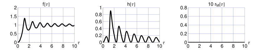
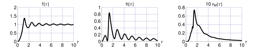
Figure 2: Positive-$\tau$ solution of the ODEs (37) for $w_{M}=1/3$ with Ansätze (39) and boundary conditions at $\tau_{\text{bcs}}=1/100$ from (40) with $\gamma=0$.

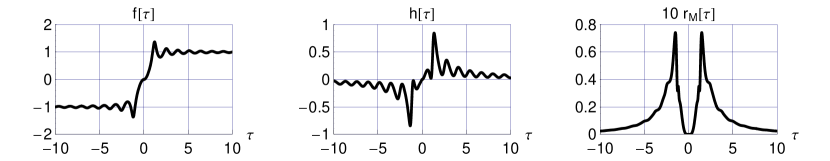
Figure 3: Same as Fig. 5 but now from the ODEs (42) with parameters $\{w_{M},\,\gamma\}=\{1/3,\,1/5\}$.

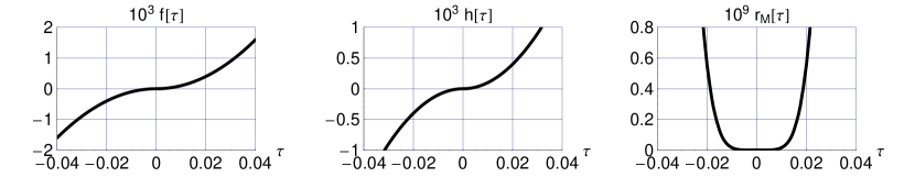
Figure 4: Positive-$\tau$ numerical solution from Fig. 5 and the corresponding negative-$\tau$ numerical solution from boundary conditions at $\tau=-\tau_{\text{bcs}}=-1/100$. The series-type solution (40) is plotted for $\tau\in[-\tau_{\text{bcs}},\,\tau_{\text{bcs}}]$, but this is barely visible for the $[-10,\,10]$ range shown (see Fig. 5 for an enlargement).

Figure 5: Solution from Fig. 5 plotted over the central region $-4\,\tau_{\text{bcs}}\leq\tau\leq 4\,\tau_{\text{bcs}}$.

Figure 6: Even solution of the cosmic scale factor $a(\tau)$ corresponding to the solutions of Fig. 5, with the series-type solution (41a) for $\tau\in[-\tau_{\text{bcs}},\,\tau_{\text{bcs}}]$ and matching boundary conditions on $a(\tau)$ at $\tau=\pm\tau_{\text{bcs}}=\pm 1/100$. The right panel shows the combination $r_{M}(\tau)\,a^{4}(\tau)$.

References

- (1) S. Weinberg, “The cosmological constant problem,” Rev. Mod. Phys. 61, 1 (1989).
- (2) F.R. Klinkhamer and G.E. Volovik, “Self-tuning vacuum variable and cosmological constant,” Phys. Rev. D 77, 085015 (2008), arXiv:0711.3170.
- (3) F.R. Klinkhamer and G.E. Volovik, “Dynamic vacuum variable and equilibrium approach in cosmology,” Phys. Rev. D 78, 063528 (2008), arXiv:0806.2805.
- (4) F.R. Klinkhamer and G.E. Volovik, “Towards a solution of the cosmological constant problem,” JETP Lett. 91, 259 (2010), arXiv:0907.4887.
- (5) F.R. Klinkhamer and G.E. Volovik, “Dynamic cancellation of a cosmological constant and approach to the Minkowski vacuum,” Mod. Phys. Lett. A 31, 1650160 (2016), arXiv:1601.00601.
- (6) F.R. Klinkhamer and G.E. Volovik, “Brane realization of -theory and the cosmological constant problem,” JETP Lett. 103, 627 (2016), arXiv:1604.06060.
- (7) F.R. Klinkhamer and G.E. Volovik, “Dark matter from dark energy in -theory,” JETP Lett. 105, 74 (2017), arXiv:1612.02326.
- (8) F.R. Klinkhamer and G.E. Volovik, “More on cold dark matter from -theory,” arXiv:1612.04235.
- (9) F.R. Klinkhamer and T. Mistele, “Classical stability of higher-derivative q-theory in the four-form-field-strength realization,” Int. J. Mod. Phys. A 32, 1750090 (2017), arXiv:1704.05436.
- (10) M. Nitta and R. Yokokura, “Topological couplings in higher derivative extensions of supersymmetric three-form gauge theories,” JHEP 05, 102 (2019), arXiv:1810.12678.
- (11) S.W. Hawking and G.F.R. Ellis, The Large Scale Structure of Space-Time (Cambridge University Press, Cambridge, England, 1973).
- (12) S.L. Sondhi, S.M. Girvin, J.P. Carini, and D. Shahar, “Continuous quantum phase transitions,” Rev. Mod. Phys. 69, 315 (1997), arXiv:cond-mat/9609279.
- (13) G.E. Volovik, “Quantum phase transitions from topology in momentum space,” in: W.G. Unruh and R. Schützhold (eds.), Quantum Analogues: From Phase Transitions to Black Holes and Cosmology, Springer Lecture Notes in Physics 718, 31 (2007), arXiv:cond-mat/0601372.
- (14) S. Sachdev, Quantum Phase Transitions, Second Edition (Cambridge University Press, Cambridge, England, 2011).
- (15) G.E. Volovik, “Exotic Lifshitz transitions in topological materials,” Phys. Usp. 61, 89 (2018), arXiv:1701.06435.
- (16) M.Z. Hasan and C.L. Kane, “Colloquium: Topological insulators,” Rev. Mod. Phys. 82, 3045 (2010), arXiv:1002.3895.
- (17) B.J. Wieder, B. Bradlyn, J. Cano, Zhijun Wang, M.G. Vergniory, L. Elcoro, A.A. Soluyanov, C. Felser, T. Neupert, N. Regnault, and B.A. Bernevig, “Topological materials discovery from crystal symmetry,” Nat. Rev. Mater. (2021), arXiv:2106.00709.
- (18) F.R. Klinkhamer, “Regularized big bang singularity,” Phys. Rev. D 100, 023536 (2019), arXiv:1903.10450.
- (19) F.R. Klinkhamer, “More on the regularized big bang singularity,” Phys. Rev. D 101, 064029 (2020), arXiv:1907.06547.
- (20) F.R. Klinkhamer and Z.L. Wang, “Nonsingular bouncing cosmology from general relativity,” Phys. Rev. D 100, 083534 (2019), arXiv:1904.09961.
- (21) F.R. Klinkhamer and Z.L. Wang, “Nonsingular bouncing cosmology from general relativity: Scalar metric perturbations,” Phys. Rev. D 101, 064061 (2020), arXiv:1911.06173.
- (22) F.R. Klinkhamer, “M-theory and the birth of the Universe,” Acta Phys. Pol. B 52, 1007 (2021), arXiv:2102.11202.
- (23) F.R. Klinkhamer, “Another model for the regularized big bang,” arXiv:2005.12157.
- (24) J. Nissinen and G.E. Volovik, “Elasticity tetrads, mixed axial-gravitational anomalies, and (3+1)-d quantum Hall effect,” Phys. Rev. Research 1, 023007 (2019), arXiv:1812.03175.
- (25) D. Gaiotto, A. Kapustin, N. Seiberg, and B. Willett, “Generalized global symmetries,” JHEP 02, 172 (2015), arXiv:1412.5148.
- (26) O. Dubinkin, A. Rasmussen, and T.L. Hughes, “Higher-form gauge symmetries in multipole topological phases,” Ann. Phys. (Amsterdam) 422, 168297 (2020), arXiv:2007.05539.
- (27) (a) M.J. Duff and P. van Nieuwenhuizen, “Quantum inequivalence of different field representations,” Phys. Lett. B 94, 179 (1980); (b) A. Aurilia, H. Nicolai, and P.K. Townsend, “Hidden constants: The theta parameter of QCD and the cosmological constant of supergravity,” Nucl. Phys. B 176, 509 (1980); (c) E. Witten, “Fermion quantum numbers in Kaluza-Klein theory,” in: Shelter Island II: Proceedings of the 1983 Shelter Island Conference on Quantum Field Theory and the Fundamental Problems of Physics, edited by R. Jackiw, N.N Khuri, S. Weinberg, and E. Witten (MIT Press, Cambridge, 1983; Dover Press, New York, 2016);
- (28) (a) S.W. Hawking, “The cosmological constant is probably zero,” Phys. Lett. B 134, 403 (1984); (b) M.J. Duff, “The cosmological constant is possibly zero, but the proof is probably wrong,” Phys. Lett. B 226, 36 (1989); (c) Z.C. Wu, “The cosmological constant is probably zero, and a proof is possibly right,” Phys. Lett. B 659, 891 (2008), arXiv:0709.3314.
- (29) (a) M. Henneaux and C. Teitelboim, “The cosmological constant as a canonical variable,” Phys. Lett B 143 (1984) 415; (b) J.D. Brown and C. Teitelboim, “Neutralization of the cosmological constant by membrane creation,” Nucl. Phys. B 297 (1988) 787; (c) M.J. Duncan and L.G. Jensen, “Four-forms and the vanishing of the cosmological constant,” Nucl. Phys. B 336, 100 (1990); (d) R. Bousso and J. Polchinski, “Quantization of four-form fluxes and dynamical neutralization of the cosmological constant,” JHEP 0006, 006 (2000), arXiv:hep-th/0004134; (e) A. Aurilia and E. Spallucci, “Quantum fluctuations of a ‘constant’ gauge field,” Phys. Rev. D 69, 105004 (2004), arXiv:hep-th/0402096.
- (30) C.D. Froggatt and H.B. Nielsen, “Standard model criticality prediction: Top mass 173 5 GeV and Higgs mass 135 9 GeV,” Phys. Lett. B 368, 96 (1996), arXiv:hep-ph/9511371.
- (31) B.G. Sidharth, A. Das, C.R. Das, L.V. Laperashvili, and H.B. Nielsen, “Topological structure of the vacuum, cosmological constant and dark energy,” Int. J. Mod. Phys. A 31, 1630051 (2016), arXiv:1605.01169.
- (32) G.E. Volovik, “Coexistence of different vacua in the effective quantum field theory and Multiple Point Principle,” JETP Lett. 79, 101 (2004), arXiv:hep-ph/0309144.
- (33) L. Boyle, K. Finn, and N. Turok, “CPT-symmetric Universe,” Phys. Rev. Lett. 121, 251301 (2018), arXiv:1803.08928.
- (34) L. Boyle and N. Turok, “Two-sheeted Universe, analyticity and the arrow of time,” arXiv:2109.06204.
- (35) L. Boyle and N. Turok, “Cancelling the vacuum energy and Weyl anomaly in the standard model with dimension-zero scalar fields,” arXiv:2110.06258.
- (36) G.E. Volovik, “Comment to the CPT-symmetric Universe: Two possible extensions,” JETP Lett. 109, 682 (2019), arXiv:1902.07584.
- (37) F.R. Klinkhamer and G.E. Volovik, “Tetrads and q-theory,” JETP Lett. 109, 364 (2019), arXiv:1812.07046.
- (38) M.A. Zubkov, “Emergent gravity in superplastic crystals and cosmological constant problem,” arXiv:1909.08412.
- (39) F.R. Klinkhamer and G.E. Volovik (unpublished).
- (40) N. Ishibashi, H. Kawai, Y. Kitazawa, and A. Tsuchiya, “A large- reduced model as superstring,” Nucl. Phys. B 498, 467 (1997), arXiv:hep-th/9612115.
- (41) H. Aoki, S. Iso, H. Kawai, Y. Kitazawa, A. Tsuchiya, and T. Tada, “IIB matrix model,” Prog. Theor. Phys. Suppl. 134, 47 (1999), arXiv:hep-th/9908038.
- (42) F.R. Klinkhamer, “IIB matrix model: Emergent spacetime from the master field,” Prog. Theor. Exp. Phys. 2021, 013B04 (2021), arXiv:2007.08485.
- (43) G.E. Volovik, The Universe in a Helium Droplet, Paperback Edition (Clarendon Press, Oxford, England, 2009).
- (44) M. Henneaux and C. Teitelboim, “The cosmological constant and general covariance,” Physics Letters B 222, 195 (1989).