The effect of boson-boson interaction on the Bipolaron formation

Abstract

Impurities immersed into a surrounding ultra-cold Bose gas experience interactions mediated by the surrounding many-body environment. If one focuses on two impurities that are sufficiently close to each other, they can form a bipolaron pair. Here, we discuss how the standard methods based on linearizing the condensate field lead to results only valid in the weak coupling regime and for sufficiently large impurity separations. We show how those shortcomings can be remedied within the Born-Oppenheimer approximation by accounting for boson-boson interactions already on the mean-field level.

I Introduction

The interaction between an impurity and a surrounding many-body environment can lead to the formation of a quasiparticle called a polaron Landau (1933); Pekar (1946). When multiple impurities are present, exchange interactions, also mediated by the surrounding environment, can lead to impurity-impurity bound states known as bipolarons. Such exchange mediated interactions are ubiquitous in physical systems, being relevant for Cooper pairs in superconductors Cooper (1956) and quark-gluon interactions Peskin and Schroeder (1995). In the solid-state context, lattice phonon vibrations are responsible for the mediated interactions. The resulting bipolarons may play a role in high-$T_{c}$ superconductivity Mott (1993); Alexandrov and Krebs (1992) and are also a vital ingredient for understanding the electric conductivity of polymers Bredas and Street (1985); Glenis et al. (1993).

In more recent years, neutral atoms immersed in ultra-cold quantum gases have provided an excellent platform to investigate the physics of polarons. Being highly tuneable via Feshbach resonances Chin et al. (2010), such systems allow access to novel regimes. Here the density fluctuations of the ultracold gas mediate the interaction between impurities which can result in a bound state as illustrated in FIG. 2. Using ultracold quantum gases, the Fermi-polaron has been investigated in a several experiments Schirotzek et al. (2009); Zhang et al. (2012); Kohstall et al. (2012); Koschorreck et al. (2012); Scazza et al. (2017); Cetina et al. (2015, 2016); Ness et al. (2020); Yan et al. (2019) and in recent years the experimental progress in Bose-polarons has also made considerable advances Catani et al. (2012); Yan et al. (2020); Jørgensen et al. (2016); Skou et al. (2021); Hu et al. (2016). A common starting point for describing impurities in an ultracold Bose gas is the linearized Fröhlich model Grusdt et al. (2015, 2015); Rath and Schmidt (2013); Li and Das Sarma (2014). Despite its applicability to the weak coupling regime, it is known from the single impurity case Ardila and Giorgini (2015); Shchadilova et al. (2016), that the Fröhlich model becomes inadequate when applied to strongly interacting impurities. A natural next step is to consider the extended Fröhlich model which systematically accounts for impurity-boson interactions of higher order, i.e. by retaining second order phonon impurity process while still neglecting phonon-phonon interaction Shchadilova et al. (2016). Although the extended Fröhlich model, has been applied with considerable success to dynamical phenomena and describing repulsive and weakly attractive interactions Shchadilova et al. (2016); Drescher et al. (2019); Ashida et al. (2018); Dzsotjan et al. (2020); Lausch et al. (2018); Ichmoukhamedov and Tempere (2019), it too possesses some significant shortcomings. For instance an instability can form due to the emergence of a bound state. The extended Fröhlich model predicts that an infinite number of bosons populates this energetically low-lying bound state which is typically unphysical Shchadilova et al. (2016). That is, in a realistic interacting Bose gas, the high occupancy of the bound state is balanced by the boson-boson repulsion Schmidt and Enss (2021); Levinsen et al. (2021). Describing the interaction between two neutral impurities immersed in a Bose gas is crucial for understanding the interplay between several impurities. Here, the Fröhlich model predicts, within the Born-Oppenheimer approximation, an attractive Yukawa potential between two impurities in 3D Naidon (2018). In Camacho-Guardian et al. (2018) it was noted however that the Yukawa potential is not entirely accurate, being only valid for weak couplings and sufficiently large impurity separation. Building on the single impurity case, one therefore might expect that the results obtained from the Frölich model for weak couplings can be improved upon in a straightforward way by including higher-order phonon impurity scattering terms. However, we will show that if one proceeds in a naive manner for two impurities, this can lead to unphysical divergences in the ground state energy due to the bound state formation between the two impurities and the excitations of the Bose gas, something that has also been demonstrated in Panochko and Pastukhov (2022). In contrast to the single impurity case, this occurs for attractive and repulsive impurity-boson scattering lengths. The mechanisms leading to this bound state are similar to those leading to the bound state formed between two localized potentials known from standard quantum mechanics Albeverio et al. (2004).

In this work, we present a conceptually simple and physically intuitive model to address the bipolaron problem. This model constitutes a good starting point for more advanced treatments and also rectifies the shortcomings of the (extended) Fröhlich model when considering the bipolaron problem. We start by introducing the full microscopic Hamiltonian. We proceed by linearizing the model and integrating out the phononic degrees of freedom which leads to the Yukawa potential. We then discuss why the Yukawa potential is inadequate and also outline why some of the standard methods used to go beyond the Fröhlich model in the single impurity case do not generalize in a straightforward manner. We then show how those problems can be remedied in a conceptually simple and intuitive way by accounting for boson-boson interaction at the mean-field level, in line with previous treatments of bipolarons in 1D Will et al. (2021); Dehkharghani et al. (2018) and single polarons Schmidt and Enss (2021); Guenther et al. (2021); Drescher et al. (2020); Jager et al. (2020); Mistakidis et al. (2019a); Brauneis et al. (2021); Koutentakis et al. (2022); Mistakidis et al. (2019b); Levinsen et al. (2021). This is done by applying the Lee-Low-Pines transformation Lee et al. (1953) and transforming to the center of mass coordinates for the two impurities. This brings the Hamiltonian into a form amenable to the Born-Oppenheimer (BO) approximation. We proceed by minimizing the resulting Gross-Pitaevskii (GP) energy functional. This leaves us with an effective Schrödinger equation for the two impurities with which we determine conditions for a bound state to occur.

II The Model

Our starting point is a microscopic theory describing two impurities coupled to a surrounding Bose gas, consisting of $N$ particles in a box of volume $V$ with periodic boundary conditions. Such a system is described by the Hamiltonian

$$\hat{\mathcal{H}} =\int\mathrm{d}^{3}r\,\hat{\phi}^{\dagger}(\mathbf{r})\bigg{(}-\frac{\nabla^{2}}{2m}+\frac{g_{\mathrm{BB}}}{2}\hat{\phi}^{\dagger}(\mathbf{r})\hat{\phi}(\mathbf{r})-\mu$$

$$+V(\mathbf{r}-\hat{\mathbf{R}}_{1})+V(\mathbf{r}-\hat{\mathbf{R}}_{2})\bigg{)}\hat{\phi}(\mathbf{r})+\frac{\hat{\mathbf{P}}_{1}^{2}+\hat{\mathbf{P}}_{2}^{2}}{2M}.$$ (1)

Here we set $\hbar=1$ and $m$ ($M$) denotes the mass of the bosons (impurity atoms), $\hat{\phi}(x)$ is the bosonic field operator describing the Bose gas, $g_{\mathrm{BB}}$ ($g_{\mathrm{IB}}$) is the boson-boson (boson-impurity) interaction strength, $\hat{\mathbf{X}}_{1,2}$ ($\hat{\mathbf{P}}_{1,2}$) denotes the position (momentum) operator of the impurities, and $\mu$ is the chemical potential of the Bose gas. The interaction between the impurities and the condensate is modelled by the interaction potential $V(\mathbf{r})$; most linearized treatments rely on employing a contact potential $V_{\delta}(\mathbf{r})=g_{\mathrm{IB}}\delta({\bf r})$ Naidon (2018); Camacho-Guardian et al. (2018). As is known for such models, when keeping the full Hamiltonian and applying a contact interaction for the impurity-boson interaction and the boson-boson interaction simultaneously, the Hamiltonian only admits zero energy (bi)polaron solutions Guenther et al. (2021). Thus when working with the non-linearized model in the Born-Oppenheimer approximation at least one of the two interactions has to be chosen to be of finite range. In this work, we employ a finite-range potential for the impurity-boson interaction. For the boson-boson interaction we still employ a contact interaction. We choose the widely-used Gaussian pseudo-potential

$$V_{\rm G}(r)=-V_{0}e^{-\frac{r^{2}}{L^{2}}},$$ (2)

with depth $V_{0}$ and range $L$ and also compare the results to the soft van-der-Waals potential

$$V_{\rm vdw}(r)=-V_{0}\frac{L^{6}}{r^{6}+L^{6}}\,.$$ (3)

The connection to the s-wave scattering length $a_{\rm IB}$ and the effective range $r_{\rm eff}$ can be made by numerically solving the two-body Schrödinger equation Jeszenszki et al. (2018); Stoof et al. (2009). For a spherical potential $u(r)$ satisfies the (radial) differential equation $\left(-\frac{\mathrm{d}^{2}}{\mathrm{d}r^{2}}+2m_{\mathrm{r}}V(r)+k^{2}\right)u_{k}(r)=0,$ where $m_{r}=mM/(m+M)$ and the boundary conditions are $u(0)=0$ and $u^{\prime}(0)=1$. By solving for $u_{k}(r)$ one can now extract the phase shift $\delta_{0}(k)$, which ultimately determines the scattering length and effective range via

$$k\cot{\delta_{0}(k)}=-\frac{1}{a_{\rm IB}}+\frac{1}{2}r_{\rm eff}k^{2}+\mathcal{O}(k^{4})\,.$$ (4)

This relation can be used to make the connection to the contact potential used in the linearized case.

To conclude this section, we introduce the relative coordinates and apply a unitary transformation to eliminate the center of mass degrees of freedom. Starting with Eq. (II), we transform into the center of mass frame and denote the relative position (momentum) of the impurities by $\hat{\mathbf{R}}$ ($\hat{\mathbf{P}}$) and the center of mass position (momentum) by $\hat{\mathbf{r}}_{\rm I}$ ($\hat{\mathbf{p}}_{\rm I}$). Subsequently we apply a Lee-Low-Pines transformation $\hat{U}=\exp(i\hat{\mathbf{r}}_{\rm I}\cdot\hat{\mathbf{P}}_{\mathrm{B}})$ ,where $\hat{\mathbf{P}}_{\mathrm{B}}=-i\int\mathrm{d}^{d}r\,\hat{\phi}^{\dagger}(\mathbf{r})\nabla\hat{\phi}(\mathbf{r})$ is the total momentum of the Bose gas. This eliminates the center of mass coordinate Will et al. (2021); Lee et al. (1953) and we arrive at the following Hamiltonian

$$\hat{\mathcal{H}}=\frac{:\left(\mathbf{p}-\hat{\mathbf{P}}_{\mathrm{B}}\right)^{2}:}{4M}+\frac{\hat{P}^{2}}{M}+\int\mathrm{d}^{3}r\,\hat{\phi}^{\dagger}(\mathbf{r})\bigg{(}\frac{-\nabla^{2}}{2m_{r}}$$ (5)

$$+\frac{g_{\mathrm{BB}}}{2}\hat{\phi}^{\dagger}(\mathbf{r})\hat{\phi}(\mathbf{r})-\mu+V(\mathbf{r}+\hat{\mathbf{R}}/2)+V(\mathbf{r}-\hat{\mathbf{R}}/2)\bigg{)}\hat{\phi}(\mathbf{r}).$$

Here, $m_{r}$ is the reduced mass and $\mathbf{p}$ is the total momentum, which is a conserved quantity and therefore can be replaced by a real number. Throughout our calculations we set $p=0$ since we focus on systems at rest to obtain the mediated interaction. One might notice that we are neglecting direct impurity-impurity interactions in our considerations. This is strictly speaking only allowed when the impurities are well separated. As will be further explained, the range of the bare impurity-impurity interaction will usually be much smaller than the range of the mediated potential. The standard procedure is to linearize the field operators and subsequently perform a Bogoliubov rotation, resulting in the (extended) Fröhlich model. The following section will briefly outline how to retrieve these results by linearizing only the density and neglecting phase-density interactions.

III Linearized theory

In this section, we address the bipolaron problem utilizing a path-integral approach, which is expanded in density fluctuations. Though the resulting expressions can be obtained directly from the Fröhlich model, the path integral approach gives a clearer picture of how the interaction is mediated by the density fluctuations of the condensate. Furthermore, it demonstrates that the neglected boson-boson interaction is the root cause of the shortcomings in predicting the mediated interactions. We start by rewriting the field operators as $\hat{\phi}(\mathbf{r})=\sqrt{n_{0}+\delta\hat{\rho}(\mathbf{r)}}e^{i\hat{\theta}(\mathbf{r})}$, where $n_{0}=\mu/g_{\mathrm{BB}}$. After performing this redefinition, dropping terms of order higher than quadratic in $\delta\rho$ and $\partial_{i}\theta$, we arrive at the imaginary-time action

$$S=\int\mathrm{d}\tau\,\Big{\{}\int\mathrm{d}^{3}r\Big{[}\delta\rho\partial_{\tau}\theta+\frac{n_{0}(\nabla\theta)^{2}}{2m_{\rm r}}+\frac{1}{2}\delta\rho\Big{(}\frac{-\nabla^{2}}{4m_{\rm r}n_{0}}$$ (6)

$$+g_{\mathrm{BB}}\Big{)}\delta\rho+g_{\mathrm{IB}}\left(\delta\rho(\mathbf{R}/2)+\delta\rho(-\mathbf{R}/2)\right)\Big{]}+\frac{\mathbf{P}^{2}}{M}\Big{\}}$$

It is now straightforward to first integrate out the density and subsequently the phase, which leaves us with an effective action for the impurities (see Ichmoukhamedov and Tempere (2019); Tempere et al. (2009) for similar calculations for the Bose polaron)

$$S=\sum_{n}\,\Big{\{}\frac{\mathbf{P}^{2}}{M}-\frac{g_{\mathrm{IB}}^{2}}{(2\pi)^{3}}\int\mathrm{d}^{3}k\,\frac{n_{0}e_{k}\cos{(\mathbf{k}\cdot\mathbf{R}/2})}{\Omega_{k}^{2}+\omega^{2}_{n}}\Big{\}}$$ (7)

where $\omega_{n}$ are Matsubara frequencies, $e_{q}=q^{2}/2m_{r}$ is the energy of the free boson and $\Omega_{q}=\sqrt{\frac{e_{q}}{2}(e_{q}+2n_{0}g_{\mathrm{BB}})}$ is the Bogoliubov dispersion. This leads to the mediated interaction

$$V_{\rm eff}(\omega_{n},\mathbf{R})=-\frac{g_{\mathrm{IB}}^{2}}{(2\pi)^{3}}\int\mathrm{d}^{3}k\,\frac{n_{0}e_{k}\cos{(\mathbf{k}\cdot\mathbf{R}/2})}{\Omega_{k}^{2}+\omega^{2}_{n}}$$ (8)

where by evaluating the momentum integral and applying the Born-Oppenheimer approximation, which allows us to take $\omega_{n}=0$, one can obtain the mediated interaction in real space. The calculations are straightforward and yield the Yukawa potential

$${V}^{\rm\delta}_{\mathrm{BP}}(R)=-\frac{4n_{0}\pi a^{2}_{\mathrm{IB}}}{m_{r}R}e^{-\sqrt{2}R/\xi}$$ (9)

where we have used the usual relation $g_{\mathrm{IB}}=\frac{2\pi}{m_{\rm r}}a_{\mathrm{IB}}$ and introduced the healing length $\xi=\frac{1}{\sqrt{2g_{\mathrm{BB}}n_{0}m_{\rm r}}}$. We note that for heavy impurities and moderate couplings, one can find the ground state energy of the biplaron by solving the resulting Schrödinger equation. For heavy impurities, one can use the generalized parametric Nikiforov–Uvarov method to calculate approximate eigenenergies for the Yukawa potential Hamzavi et al. (2012), which results in the ground state energy

$$E^{\rm\delta}_{BP}=-4\pi^{2}\frac{Mn_{0}^{2}a_{\mathrm{IB}}^{4}}{m_{\rm r}^{2}}.$$ (10)

We note that this bound state only exists when $|a_{\mathrm{IB}}|\geq\sqrt{\frac{m_{\rm r}}{\sqrt{2}Mn_{0}\pi\xi}}$ Hamzavi et al. (2012). One can already see a major shortcoming of this approach, namely the bound state energy scales linearly in $M$ and the bipolaron energy diverges for $M\rightarrow\infty$. This is unphysical. The diverging energy can be traced back to the fact that the Yukawa potential is unbounded from below, and for $M\rightarrow\infty$, the kinetic energy becomes irrelevant. The unboundedness of the mediated interaction is a direct consequence of the delta function constituting a zero-range potential and therefore requires regularization. The regularization employed for the delta function regularizes the scattering for each impurity separately and is valid as long as the particles have non-zero separation, but breaks down when the impurities sit on top of each other, which effectively constitutes a single impurity with twice the bare interaction. Hence the ground-state energy becomes proportional to the minimum of the potential, which is $-\infty$ for the Yukawa potential. Additionally this treatment predicts a divergence at the Feshbach resonance. Repulsive boson-boson interaction prevents an infinite number of bosons from attaching to the impurity, due to internal pressure arising from an increased number of bosons in a finite volume and we thus we do not expect such a divergence when accounting for boson-boson interactions.

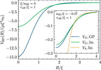
Figure 1: The mediated potential for the two impurities near the Feshbach resonance. We can see that the transition for a more realistic pseudo-potential is smooth across the resonance. In contrast the diverging scattering length leads to a breakdown of the Yukawa predictions. It also becomes clear that for larger $a_{\mathrm{IB}}$, the Fröhlich model, even with a UV regulated pseudo-potential, becomes inadequate. The inset shows the mediated interaction potential for small $a_{\mathrm{IB}}$ (corresponding to small $V_{0}$). Here we can see that the linearized theory and the GP results agree fairly well. Additionally it should be noted that the Yukawa potential obtained by using a regularized contact interaction is only accurate for large separations.

In principle, one can improve upon these results by expanding the action perturbatively and resumming certain classes of diagrams. However, as shown in Schmidt and Enss (2021) for the case of a single impurity, this is strictly speaking beyond the validity of the model and can lead to unphysical results near the scattering resonance due to the breakdown of the model associated with the bound state formation. In Appendix A, we show with the help of the extended Fröhlich model for two impurities, that this can be problematic and can lead to divergences in the mediated potential. The idea is simple, in analogy with the case of a single particle interacting with two delta potentials (see Albeverio et al. (2004) and Appendix B), a bound state can form between the excitations and the two impurities. This bound state is energetically favorable and, without phonon-phonon interaction preventing an accumulation in this state, the condensate breaks down. To alleviate those problems, one has to incorporate phonon-phonon interaction and employ an interaction potential with finite range. The following section describes how this can be done by considering the boson-boson interaction at the mean-field level.

Repeating the above analysis using the Gaussian potential (instead of a contact potential), one finds

$$V^{\rm G,\,lin}_{\mathrm{BP}}(R)=-\frac{2V^{2}_{0}L^{6}\pi m}{R}\times\\ \int^{\infty}_{0}\frac{\sin(qR)n_{0}q}{q^{2}+2/\xi^{2}}\exp\left(-q^{2}L^{2}/2\right)\,\mathrm{d}q.$$ (11)

Note that with this potential, $V^{\mathrm{Gauss}}_{\mathrm{BP}}$ stays finite for small $R$. This can be understood by noting that the exponential cut-off $\exp\left(-q^{2}L^{2}/2\right)$ is an effective UV-regulator, which is absent in the case of a delta function potential. However, if one uses this scattering potential for the extended Fröhlich model, the bound state problem will persist. Additionally, the model loses the appeal of being analytically tractable when including higher-order phonon terms. To summarize, while both (9) and(11) are obtained by linearizing the model only (9) assumes a contact potential and is thus ill-defined for $R=0$

IV Main methodology and results

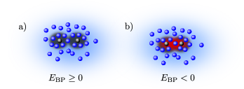
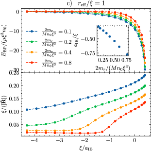
Figure 2: a) Schematic of bipolaron formation. If the interaction strength is weak or the impurities are very light, no bound state is formed, and only two polarons coexist. b) For strong enough interactions, a bound state called the bipolaron emerges. c) The binding energy and inverse separation of the bipolaron for different impurity kinetic energy scales as a function of the inverse scattering length. The separation of the impurities is defined through $\langle|\mathbf{\hat{R}}|\rangle=\langle|\mathbf{\hat{R}}_{1}-\mathbf{\hat{R}}_{2}|\rangle$.The results are for $r_{\mathrm{eff}}=1$ and obtained using $V_{\rm G}$. From the inverse separation it can clearly be seen when a bound state (the bipolaron) is formed. This threshold decreases with $\frac{m_{\rm r}}{Mn_{0}\xi^{3}}$ and in fact becomes $0$ for $\frac{m_{\rm r}}{Mn_{0}\xi^{3}}=0$. In the inset we show the scattering length threshold after which a bound state is formed as a function of the mass ratio.

In this section, we describe an approach which eliminates the difficulties encountered in the previous section. The Hamiltonian (5) will serve as the starting point for the mean-field treatment. The GP energy functional in the BO approximation that needs to be minimized to find the ground state can now be simply read off from (5)

$$E(\phi,\mathbf{R})= \int\mathrm{d}^{3}r\,\Bigg{\{}\frac{|\nabla\phi|^{2}}{2m_{\rm r}}+\frac{g_{\mathrm{BB}}}{2}(|\phi|^{2}-n_{0})^{2}$$ (12)

$$+\left({V}(\mathbf{r}+\mathbf{R/2})+{V}(\mathbf{r}-\mathbf{R/2})\right)|\phi|^{2}\Bigg{\}}.$$

To minimize the energy functional we have used the split-step Fourier algorithm in imaginary time . This, in turn, allows us to calculate the mediated interaction through

$$V^{\rm GP}_{\rm BP}(R)=E(R)-E_{0}-E(\infty),$$ (13)

where $E_{0}$ is the energy of the Bose gas without impurities and $E(\infty)$ is the energy of the two polarons at infinite separation and is subtracted to obtain the purely attractive part attributed to the bipolaron. Before discussing the main results we want to show that the problem can in fact be characterised by a few re-scaled parameters, which can then be used to interpret the results in terms of experimentally observable quantities. First we note that the chemical potential can be written as $\mu=\frac{4\pi a_{\mathrm{BB}}}{m_{\mathrm{r}}}n_{0}$. By rescaling $\phi\rightarrow\phi\sqrt{n_{0}}$, $r\rightarrow r\xi$ and $V\rightarrow V/\mu$ we then find

$$\frac{E(\phi,\mathbf{R})}{\mu\xi^{3}n_{0}}= \int\mathrm{d}^{3}r\,\Bigg{\{}|\nabla\phi|^{2}+\frac{1}{2}(|\phi|^{2}-1)^{2}$$ (14)

$$+\left({V}(\mathbf{r}+\mathbf{R/2})+{V}(\mathbf{r}-\mathbf{R/2})\right)|\phi|^{2}\Bigg{\}}\,.$$

Which shows that within the validity of of the c-field treatment our results are characterised only by the re-scaled energy, interaction strength, and impurity mass.

In FIG. 1 we show the shape of the mediated potential between two impurities for different $a_{\rm IB}$. The inset shows the comparison with the linearized model for weak coupling; here, we chose the s-wave scattering length of the Yukawa potential to match the scattering length of the Gaussian potential. For weak coupling, there is good quantitative agreement between the linearized model using a Gaussian pseudo-potential and the result obtained using the GP functional (see inset). We also observe that the Yukawa potential, which is obtained by employing a zero-range interaction, matches the behavior of the interaction potential with finite range for larger separations, indicating that the exact effective range of the potential is not highly relevant for the range of the mediated potential. One main difference between a zero range interaction and a more realistic Gaussian interaction is that the mediated potential stays finite for $R=0$. A similar discrepancy between the Yukawa potential and the mediated potential was reported in Camacho-Guardian et al. (2018) using a scattering matrix approach.

In FIG. 1 we also show the mediated interaction close to the Feshbach resonance. Here another shortcoming of the zero range scattering potential is revealed, namely close to the scattering resonance $a_{\mathrm{IB}}$ diverges, leading to infinite attraction, which is unphysical. The results obtained from the GP energy functional and the result obtained employing a Gaussian potential give a more realistic picture. Here, the mediated interaction changes less drastically across the Feshbach resonance. We also note that for larger $a_{\rm IB}$ (corresponding to larger $V_{0}$), the linearization approach becomes inadequate and significant deviation from the GP result can be observed. While the Fröhlich model with Gaussian potential underestimates the interaction here, we note that it is not a priori clear whether the Fröhlich model overestimates or underestimates the mediated potential. The two competing effects that the Fröhlich model does not account for are (i) two and higher-order phonon impurity scattering processes, which lead to enhanced mediated impurity-impurity interaction and (ii) the boson-boson interaction, which damps the phonon exchange. We can see that changing $a_{\rm BB}$, while keeping all other parameters constant effectively results in re-scaling the impurity boson scattering length. Thus we move from the situation depicted in the inset of FIG. 1 to the one shown in the main part of FIG. 1. This is exactly what one would expect, by noting that for large boson-boson interaction higher order phonon terms are damped out quickly and by neglecting the damping in the Fröhlich model we overestimate the mediated interaction.

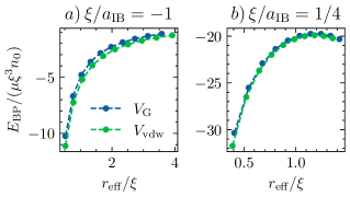
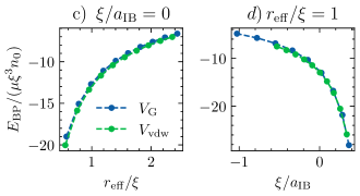
Figure 3: a),b),c): The bipolaron energy for different $a_{\mathrm{IB}}$ as a function of the effective range $r_{\rm eff}$. In d), the effective range is fixed and the bipolaron energy is plotted as a function of inverse scattering length. The plots demonstrate that the bipolaron energy is almost completely determined by the scattering length and the effective range and using different underlying potentials leads to similar results. All curves are for the $M=\infty$ case.

The bipolaron energy can be calculated by finding the ground-state of the resulting stationary Schrödinger equation. We note that within the mean-field approximation for $p=0$, the wave function $\phi$ can always be chosen to be real. Therefore we do not have to consider the vector-potential typically arising within the Born-Oppenheimer approximation Wilczek and Shapere (1989). Moreover, we observe that the equation is radially symmetric and that the ground-state will have zero angular momentum. Hence, we have to solve the following radial Schrödinger equation to obtain the bipolaron energy

$$\left(-\frac{1}{M}\frac{\mathrm{d}^{2}}{\mathrm{dR^{2}}}+V^{\mathrm{GP}}_{\mathrm{BP}}(R)\right)u(R)=E_{\mathrm{BP}}u(R),$$ (15)

with the boundary condition $u(0)=0$. The results obtained are shown in FIG. 2. We note that strictly speaking, our approach is only valid for $m/M\ll 1$. This corresponds to a vanishing impurity kinetic energy scale $\frac{m_{\rm r}}{Mn_{0}\xi^{3}}$, which serves as a control parameter for the Born-Oppenheimer approximation. It is notable that the dependence on the mass ratio is weak compared to the linearized case (compare with (10), where the energy scales linearly in the impurity mass), which can be explained by realizing that the effective potential stays finite. This can be understood by comparing kinetic energy to the potential energy. If the mass ratio becomes small, the kinetic energy becomes less important, and the solution of (15) will be localized around the minimum of the potential. Furthermore, we observe a critical $a_{\mathrm{IB}}$ after which a bipolaron characterized by $E_{\mathrm{BP}}<0$) is formed, see d, see also the inset of FIG. 2. In FIG. 2 this can also be clearly identified from the inverse separation of the impurities. We also note that the transition across the scattering resonance is smooth and the bipolaron binding energy further increases after crossing the scattering resonance. This can be understood by noting that the amplitude of the mediated potential $V^{\mathrm{GP}}_{\mathrm{BP}}$ increases further after crossing the resonance. Additionally, for heavy impurities the binding energy is approximately related to polaron energy through the approximate relationship $E_{BP}\approx E_{pol}(2V_{0})-2E_{pol}(V_{0})$, which becomes exact in the limit $M\rightarrow\infty$, since here the impurity kinetic energy becomes negligible and thus $\langle|\hat{\mathbf{R}}|\rangle\rightarrow 0$. Since in the regime after crossing the resonance the polaron energy scales faster than linearly Schmidt and Enss (2021); Levinsen et al. (2021) we expect the bipolaron binding energy to increase further across the resonance. We remark that the above argument relies on the validity of the GP treatment. In fact for $a_{\mathrm{IB}}>0$ two body bound states can appear that invalidate the GP treatment and while a detailed study of this regime is beyond the scope of this work it could be an interesting direction for further studies.

In FIG. 3 we show the bipolaron energy for the $M=\infty$ case for two different impurity-boson interaction potentials. Namely, we compare a Gaussian potential with the soft van-der-Waals potential. Here we either fix the effective range or the scattering length. We find that on either side of the scattering resonance and at the resonance the exact shape of the potential does not influence the results considerably and the exact choice of the underlying potential is not highly relevant for the obtained bipolaron energy. Interestingly, the bipolaron binding energy increases with a decreasing effective range. In FIG. 3 d) we show the binding energy across the resonance for fixed effective range and we can see that the binding energy across the resonance is smooth.

In FIG. 4 we show the separation of the impurities and the bipolaron binding energy for different mass ratios as a function of the effective range for a) $\xi/a_{\mathrm{IB}}=-1$ and b) $\xi/a_{\mathrm{IB}}=0$. As in the infinite mass case we observe, that energy decreases with the effective range. Additionally we see that impurity separation defined trough $\langle|\mathbf{\hat{R}}|\rangle=4\pi\int^{\infty}_{0}\mathrm{d}{R}\,R|u(R)|^{2}$ stays of the order of the effective range of the underlying interaction potential.

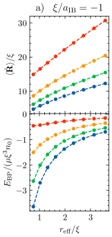
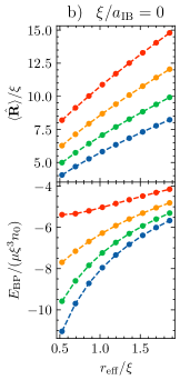
Figure 4: The effective range dependence of the bipolaron energy and size the for different mass ratios and a) $\xi/a_{\mathrm{IB}}=-1$ and b) $\xi/a_{\mathrm{IB}}=0$. All results are obtained using $V_{\rm G}$ and the colors indicate the same values as in FIG. 2. As expected the separation of the impurities increases with the effective range of the potential and also for lighter impurities. The bipolaron binding energy decreases with increasing effective range and for lighter impurities.

As mentioned earlier, it is essential to compare the localization of this bound state to the range of the direct impurity-impurity interaction. Here we note that, on average, the separation is much greater than the range of the direct impurity-impurity interaction, which in this case is actually the important length scale since after integrating out the bosonic degrees of freedom, we have reduced the problem effectively to a single particle scattering problem, with two competing length scales. To make this statement a bit more quantitative, we compare some characteristic effective ranges. Considering a microscopic van-der-Waals interaction the effective range is given by $r_{0}\sim(C_{6}m/m_{e})^{1/4}a_{0}$ Pethick and Smith (2008) , where $a_{0}$ is the Bohr radius and typical values are $C_{6}\sim 10^{3}$ and $m/m_{e}\sim 10^{4}-10^{5}$, which gives the estimate $r_{0}\sim 100a_{0}$. To put this into context, one can estimate the healing length in terms of the Bohr radius for typical experimental values (see for example Yan et al. (2020)), which leads to $\xi\sim 10^{7}-10^{10}a_{0}$. Hence the effective range of the direct impurity-impurity interaction typically a fraction of the range of the effective interaction potential mediated by the condensate. In FIG. 4 it can also be clearly seen that the separation of the impurities is much larger than the effective range of the direct impurity impurity interaction. In the case of large impurity-bath interactions, the direct impurity-impurity interaction can no longer be neglected, and few-body physics, like the bound state between the two impurities due to direct impurity-impurity interaction, can become relevant.

V Conclusion

We have presented an approach to the ground-state interaction of two impurities immersed into a three dimensional Bose gas capable of taking the boson-boson interaction into account. We started by showing that linearization efforts and the resulting Fröhlich Hamiltonian are inadequate to fully describe the polaron interaction in a Bose gas. We also discussed how naive extensions of the Fröhlich model are inadequate. We then outlined how these issues can be addressed using a mean-field treatment paired with the Born-Oppenheimer approximation. The Born-Oppenheimer approximation is valid for heavy impurities. While strictly speaking, the mean-field approximation neglects quantum corrections in the form of modified phonons completely, it is important to note that the bipolaron properties are determined by short-scale physics. Therefore, we do not expect the modified phonons, which arise when including quantum corrections to play a significant role in this regime. We first minimized the mean-field energy functional, from which we extracted the interaction potential. Here, we compared our results to the Yukawa potential and the results obtained from the linearized model with a Gaussian potential. We then calculated the bipolaron energy using the effective potential by solving the resulting radial Schrödinger equation. A detailed comparison of the results presented here with other methods and especially with the quasi-exact quantum Monte Carlo method would be a very interesting direction for future work. The work highlights the fundamental problems like diverging mediated interactions, associated with approaches based on linearization when studying the interplay of two impurities and shows a simple way of dealing with these shortcomings. We hope that the methods presented will serve as fertile ground to explore the bipolaron in and out of equilibrium in greater detail.

References

- Landau (1933) L. Landau, Phys. Z. Sowjetunion 3, 644 (1933).
- Pekar (1946) S. Pekar, Zh. Eksp. Teor. Fiz. 16 (1946).
- Cooper (1956) L. N. Cooper, Phys. Rev. 104, 1189 (1956).
- Peskin and Schroeder (1995) M. E. Peskin and D. V. Schroeder, An Introduction to quantum field theory (Addison-Wesley, Reading, USA, 1995).
- Mott (1993) N. Mott, Phys. C Supercond. 205, 191 (1993).
- Alexandrov and Krebs (1992) A. S. Alexandrov and A. B. Krebs, Sov. Phys. - Uspekhi 35, 345 (1992).
- Bredas and Street (1985) J. L. Bredas and G. B. Street, Acc. Chem. Res. 18, 309 (1985).
- Glenis et al. (1993) S. Glenis, M. Benz, E. LeGoff, M. G. Kanatzidis, J. L. Schindler, and C. R. Kannewurf, J. Am. Chem. Soc. 115, 12519 (1993).
- Chin et al. (2010) C. Chin, R. Grimm, P. Julienne, and E. Tiesinga, Rev. Mod. Phys. 82, 1225 (2010).
- Schirotzek et al. (2009) A. Schirotzek, C. H. Wu, A. Sommer, and M. W. Zwierlein, Phys. Rev. Lett. 102, 230402 (2009).
- Zhang et al. (2012) Y. Zhang, W. Ong, I. Arakelyan, and J. E. Thomas, Phys. Rev. Lett. 108, 235302 (2012).
- Kohstall et al. (2012) C. Kohstall, M. Zaccanti, M. Jag, A. Trenkwalder, P. Massignan, G. M. Bruun, F. Schreck, and R. Grimm, Nature 485, 615 (2012).
- Koschorreck et al. (2012) M. Koschorreck, D. Pertot, E. Vogt, B. Fröhlich, M. Feld, and M. Köhl, Nature 485, 619 (2012).
- Scazza et al. (2017) F. Scazza, G. Valtolina, P. Massignan, A. Recati, A. Amico, A. Burchianti, C. Fort, M. Inguscio, M. Zaccanti, and G. Roati, Phys. Rev. Lett. 118, 083602 (2017).
- Cetina et al. (2015) M. Cetina, M. Jag, R. S. Lous, J. T. Walraven, R. Grimm, R. S. Christensen, and G. M. Bruun, Phys. Rev. Lett. 115, 135302 (2015).
- Cetina et al. (2016) M. Cetina, M. Jag, R. S. Lous, I. Fritsche, J. T. Walraven, R. Grimm, J. Levinsen, M. M. Parish, R. Schmidt, M. Knap, and E. Demler, Science 354, 96 (2016).
- Ness et al. (2020) G. Ness, C. Shkedrov, Y. Florshaim, O. K. Diessel, J. Von Milczewski, R. Schmidt, and Y. Sagi, Phys. Rev. X 10, 041019 (2020), arXiv:2001.10450 .
- Yan et al. (2019) Z. Yan, P. B. Patel, B. Mukherjee, R. J. Fletcher, J. Struck, and M. W. Zwierlein, Phys. Rev. Lett. 122, 093401 (2019), arXiv:1811.00481 .
- Catani et al. (2012) J. Catani, G. Lamporesi, D. Naik, M. Gring, M. Inguscio, F. Minardi, A. Kantian, and T. Giamarchi, Phys. Rev. A 85, 023623 (2012).
- Yan et al. (2020) Z. Z. Yan, Y. Ni, C. Robens, and M. W. Zwierlein, Science 368, 190 (2020).
- Jørgensen et al. (2016) N. B. Jørgensen, L. Wacker, K. T. Skalmstang, M. M. Parish, J. Levinsen, R. S. Christensen, G. M. Bruun, and J. J. Arlt, Phys. Rev. Lett. 117, 055302 (2016).
- Skou et al. (2021) M. G. Skou, T. G. Skov, N. B. Jørgensen, K. K. Nielsen, A. Camacho-Guardian, T. Pohl, G. M. Bruun, and J. J. Arlt, Nat. Phys. 17, 731 (2021).
- Hu et al. (2016) M. G. Hu, M. J. Van De Graaff, D. Kedar, J. P. Corson, E. A. Cornell, and D. S. Jin, Phys. Rev. Lett. 117, 055301 (2016).
- Grusdt et al. (2015) F. Grusdt, Y. E. Shchadilova, A. N. Rubtsov, and E. Demler, Sci. Rep. 5 (2015), 10.1038/srep12124, arXiv:1410.2203 .
- Rath and Schmidt (2013) S. P. Rath and R. Schmidt, Phys. Rev. A 88, 053632 (2013).
- Li and Das Sarma (2014) W. Li and S. Das Sarma, Phys. Rev. A 90, 013618 (2014).
- Ardila and Giorgini (2015) L. A. Ardila and S. Giorgini, Phys. Rev. A 92, 33612 (2015).
- Shchadilova et al. (2016) Y. E. Shchadilova, R. Schmidt, F. Grusdt, and E. Demler, Phys. Rev. Lett. 117, 113002 (2016).
- Drescher et al. (2019) M. Drescher, M. Salmhofer, and T. Enss, Phys. Rev. A 99, 023601 (2019).
- Ashida et al. (2018) Y. Ashida, R. Schmidt, L. Tarruell, and E. Demler, Phys. Rev. B 97, 060302 (2018).
- Dzsotjan et al. (2020) D. Dzsotjan, R. Schmidt, and M. Fleischhauer, Phys. Rev. Lett. 124, 223401 (2020).
- Lausch et al. (2018) T. Lausch, A. Widera, and M. Fleischhauer, Phys. Rev. A 97, 33620 (2018).
- Ichmoukhamedov and Tempere (2019) T. Ichmoukhamedov and J. Tempere, Phys. Rev. A 100, 043605 (2019).
- Schmidt and Enss (2021) R. Schmidt and T. Enss, (2021), arXiv:2102.13616v1 .
- Levinsen et al. (2021) J. Levinsen, L. A. P. Ardila, S. M. Yoshida, and M. M. Parish, Phys. Rev. Lett. 127, 33401 (2021).
- Naidon (2018) P. Naidon, J. Phys. Soc. Japan 87, 043002 (2018).
- Camacho-Guardian et al. (2018) A. Camacho-Guardian, L. A. Peña Ardila, T. Pohl, and G. M. Bruun, Phys. Rev. Lett. 121, 013401 (2018).
- Panochko and Pastukhov (2022) G. Panochko and V. Pastukhov, Atoms 10, 19 (2022).
- Albeverio et al. (2004) S. Albeverio, F. Gesztesy, R. Høegh-Krohn, and H. Holden, Solvable Models in Quantum Mechanics (American Mathematical Society, Providence, Rhode Island, 2004).
- Will et al. (2021) M. Will, G. E. Astrakharchik, and M. Fleischhauer, Phys. Rev. Lett. 127, 103401 (2021).
- Dehkharghani et al. (2018) A. S. Dehkharghani, A. G. Volosniev, and N. T. Zinner, Phys. Rev. Lett. 121, 080405 (2018).
- Guenther et al. (2021) N. E. Guenther, R. Schmidt, G. M. Bruun, V. Gurarie, and P. Massignan, Phys. Rev. A 103, 013317 (2021).
- Drescher et al. (2020) M. Drescher, M. Salmhofer, and T. Enss, Phys. Rev. Res. 2, 032011 (2020).
- Jager et al. (2020) J. Jager, R. Barnett, M. Will, and M. Fleischhauer, Phys. Rev. Res. 2, 033142 (2020).
- Mistakidis et al. (2019a) S. I. Mistakidis, G. C. Katsimiga, G. M. Koutentakis, T. Busch, and P. Schmelcher, Phys. Rev. Lett. 122, 183001 (2019a).
- Brauneis et al. (2021) F. Brauneis, H. W. Hammer, M. Lemeshko, and A. G. Volosniev, SciPost Phys. 11, 8 (2021).
- Koutentakis et al. (2022) G. M. Koutentakis, S. I. Mistakidis, and P. Schmelcher, Atoms 10, 3 (2022).
- Mistakidis et al. (2019b) S. I. Mistakidis, A. G. Volosniev, N. T. Zinner, and P. Schmelcher, Phys. Rev. A 100, 013619 (2019b).
- Lee et al. (1953) T. D. Lee, F. E. Low, and D. Pines, Phys. Rev. 90, 297 (1953).
- Jeszenszki et al. (2018) P. Jeszenszki, A. Y. Cherny, and J. Brand, Phys. Rev. A 97, 042708 (2018).
- Stoof et al. (2009) H. T. Stoof, K. B. Gubbels, and D. B. Dickerscheid, Theor. Math. Phys. 2009, 475 (2009).
- Tempere et al. (2009) J. Tempere, W. Casteels, M. K. Oberthaler, S. Knoop, E. Timmermans, and J. T. Devreese, Phys. Rev. B 80, 184504 (2009).
- Hamzavi et al. (2012) M. Hamzavi, M. Movahedi, K. E. Thylwe, and A. A. Rajabi, Chinese Phys. Lett. 29, 080302 (2012).
- Note (1) All calculations were performed in Cartesian coordinates, and to speed up the calculations, they were performed on GPUs using CUDA.jl Besard et al. (2019).
- Wilczek and Shapere (1989) F. Wilczek and A. Shapere, Geometric Phases in Physics (WORLD SCIENTIFIC, 1989).
- Pethick and Smith (2008) C. J. Pethick and H. Smith, Bose-Einstein Condensation in Dilute Gases, Vol. 9780521846 (Cambridge University Press, 2008).
- Fröhlich (1954) H. Fröhlich, Adv. Phys. 3, 325 (1954).
- Grusdt et al. (2017) F. Grusdt, G. E. Astrakharchik, and E. Demler, New J. Phys. 19, 103035 (2017).
- Killingbeck (1987) J. Killingbeck, J. Phys. A. Math. Gen. 20, 1411 (1987).
- Lagaris et al. (1998) I. E. Lagaris, A. Likas, and D. I. Fotiadis, IEEE Trans. Neural Networks 9, 987 (1998).
- Lagaris et al. (2000) I. E. Lagaris, A. C. Likas, and D. G. Papageorgiou, IEEE Trans. Neural Networks 11, 1041 (2000).
- Li et al. (2021) H. Li, Q. Zhai, and J. Z. Chen, Phys. Rev. A 103, 32405 (2021).
- Besard et al. (2019) T. Besard, C. Foket, and B. De Sutter, IEEE Trans. Parallel Distrib. Syst. 30, 827 (2019).