Measurements of the Expansion Velocities of Ionized-Gas Superbubbles in Nearby Galaxies Based on Integral Field Spectroscopy Data

Abstract

The study of dynamic properties of bubbles in the interstellar medium is important for understanding the feedback mechanisms from star-formation processes in galaxies. The ongoing integral field spectroscopy of nearby star-forming galaxies reveals many expanding bubbles and superbubbles identified by the local increase in gas velocity dispersion. The limited angular resolution often prevents bona fide measures of the expansion velocities in galaxies outside the Local Group, even despite sufficient spectroscopic resolution. We present a method that makes it possible to measure the expansion velocity of bubbles surrounding massive stars and clusters based on the data about local variations in gas velocity dispersion. We adapt the method for the Fabry–Perot interferometers used with the 6-m telescope of the Special Astrophysical Observatory of the Russian Academy of Sciences, as well as for any integral field spectrograph with a Gaussian line spread function. We apply the method described to analyze the kinematics of ionized superbubbles gas and the only known supernova remnant in the IC 1613 galaxy. The estimate of the kinematic age of the supernova remnant (on the order of 3100 years) agrees well with the previously obtained independent estimate based on X-ray data.

1 INTRODUCTION

Stars with masses $M>8~{}M_{\odot}$ play an important role in the evolution of the interstellar medium in galaxies. Their wind, ionizing radiation, and subsequent supernova explosions are the source of energy for the formation of shell-like structures surrounding clusters and OB-associations. The sizes of the observed bubbles vary over a wide range—from several parsecs to several hundred parsecs in the case of supershells/superbubbles (Oey and Clarke, 1997; Nath et al., 2020). Sustained energy inflow from several generations of stars results in further growth of superbubbles to sizes of 1–3 kpc (Weisz et al., 2009; Warren et al., 2011). In some dwarf galaxies such giant superbubbles are the dominant structure of the interstellar medium (Egorov et al., 2018). Such superbubbles that are larger than a few hundred parsecs are mostly observed in H I at 21 cm (Bagetakos et al., 2011), although deep images in emission lines allow detection of similar structures in ionized gas (Egorov et al., 2014, 2017).

The classical model of the evolution of bubbles driven by the winds of massive stars (Weaver et al., 1977) and the combined wind of multiple stars and supernova explosions (Mac Low and McCray, 1988) describes the observed structures in the interstellar medium of galaxies quite well at qualitative level. According to this model, the radius of a bubble $R$ depends on time $t$ and the inflow of mechanical energy $L$ as $R\sim L^{1/5}t^{3/5}$. Accordingly, at each moment of time its expansion velocity is $v_{\rm exp}\sim L^{1/5}t^{-2/5}$. Thus the age of the bubble and the energy required for its formation can be estimated based on the observed quantities—the size and expansion velocity. In particular, the age of the shell can be estimated in terms of the Weaver et al. (1977) model as $t=0.6R/v_{\rm exp}$. Because of this rather simple analytical dependence the observed parameters of superbubbles in nearby galaxies can serve as indicators of the properties of massive stars responsible for the formation of these structures. However, a numerical comparison of observed superbubbles properties with their estimates predicted by the (Weaver et al., 1977) model showed a severalfold-factor discrepancy (Oey and García-Segura, 2004). Radiative energy losses, which can range from 60% to almost 100% (Sharma et al., 2014; Vasiliev et al., 2015a; Yadav et al., 2017), are viewed as one of the main causes of this discrepancy. The new analytical model of superbubble evolution proposed by El-Badry et al. (2019) takes this factor into account as a parameter. However, it remains an open question how the efficiency of energy transfer from star clusters into the mechanical energy of expanding superbubbles changes under different conditions (e.g., in the case of different metallicities and gas densities).

The development of integral field spectroscopy techniques has made possible a detailed comparison of observed properties of massive stars and of the surrounding regions of ionized gas in several nearby galaxies, allowing the contribution of various feedback processes to the overall process of energy and momentum exchange with the interstellar medium to be estimated (Egorov et al., 2014, 2017; McLeod et al., 2019; Ramachandran et al., 2019; McLeod et al., 2020). However, such studies are significantly limited by the spatial and spectroscopic resolution of observational data. Thus with the characteristic sizes of the shells surrounding individual massive stars or small OB-associations on the order of several tens of parsecs, even at a distance of 4–5 Mpc (e.g., the M 81 group (Karachentsev et al., 2013)) the angular sizes of such objects often become comparable to the angular resolution of observational data (on the order of $2\arcsec$–$3\arcsec$), making the determination of superbubbles sizes and expansion velocities quite a challenging task. Furthermore, the characteristic observed superbubbles expansion velocities 20-50 km s^-1 make it impossible for most modern integral field spectrographs to resolve the emission line profiles into components to reliably estimate their expansion velocities. Observations of a number of nearby dwarf galaxies made with the Fabry–Perot interferometer (FPI) in the H$\alpha$ line demonstrate the presence of a substantial number of regions of increased ionized gas velocity dispersion whose position on the “intensity–velocity dispersion” diagram ($I$–$\sigma$) allows us to interpret them as spectroscopically unresolved expanding superbubbles (Moiseev and Lozinskaya, 2012). Numerical simulations of the interaction of multiple supernova remnants yield a close to the observed pattern in the ($I$–$\sigma$) parameter space, which confirms the above interpretation (Vasiliev et al., 2015b). As shown by Guerrero et al. (1998), such superbubbles should exhibit radial gradient of the emission line profile width, which can be used to estimate the expansion velocity, however, such measurements require a rather high angular resolution. On the other hand, Tenorio-Tagle et al. (1996) showed that the presence of a spatially unresolved shell also broadenes the observed emission line profile. In particular, Moiseev and Lozinskaya (2012) proposed to use this effect to search for unique emission objects with high stellar wind speeds (e.g., Wolf-Rayet stars, luminous blue variables) on the ($I$–$\sigma$) dependence for the galaxies studied. Thus, even in cases of insufficient spatial and spectroscopic resolution, expanding bubbles around stars and clusters can be identified by changes in the width of the spectral line profile. However, the physical parameters of such bubble (in particular, its expansion velocity) often cannot be estimated directly without invoking model assumptions about its geometry.

In this paper, we propose a method that allows us to estimate the expansion velocity of the bubbles and superbubbles in the interstellar medium from measurements of the emission line profile width in their integrated spectra and from the average velocity dispersion of the interstellar medium in the galaxy. The method is based on the analytical model of a uniform spherically symmetric expanding shell in the turbulent interstellar medium, however we show that the estimates are also valid for the case of non-uniform shells, and agree well with “direct” measurements of the expansion velocities and ages of observed superbubbles and supernova remnants (based on the example of the IC 1613 galaxy). The method described above is applicable, in particular, to spatially unresolved (or poorly resolved) shells, as well as in the cases where spectroscopic resolution prevents decomposition of the line profile into kinematically isolated components. In this paper we consider two types of spectrographs: with an instrumental profile (line spread function, LSF) in the form of a Lorentz function (as in FPI) and with a Gaussian instrumental profile (applicable to the case of many classical integral field spectrographs). We have considered Lorentzian LSF widths corresponding to the FPIs used in SCORPIO-2 (Afanasiev and Moiseev, 2011) focal reducer of the 6-m telescope of the Special Astrophysical Observatory of the Russian Academy of Sciences (SAO RAS) (see review of the method in Moiseev et al., 2021).

This paper has the following layout. Section 2 describes the analytical model of a uniform expanding bubble in a turbulent medium and the factors that affect the shape of its integrated emission line profile (turbulence of the interstellar medium, thermal and instrumental broadening), and provides a qualitative comparison of the constructed model with the H$\alpha$ line profiles of observed objects. Section 3 describes the proposed method for measuring the expansion velocity of a bubble from the observed velocity dispersion, and the results of its Monte Carlo testing. In Section 4, we use the method described above to estimate the expansion velocity of the expanding superbubble of ionized gas in IC 1613 and determine the kinematic age of the only supernova remnant in this galaxy. We summarize the main conclusions of this work in Section 5.

2 MODELING THE PROFILE OF AN EXPANDING BUBBLE

2.1 A Uniform Expanding Bubble in Unperturbed Interstellar Medium

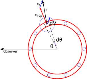
Figure 1: Scheme of a uniform expanding bubble model. The velocity of an emitting atom from spherical layer $dV$ with polar angle $\theta$ relative to the center of the shell is equal to the sum of the bubble expansion velocity $v_{\rm exp}$ (red) and the random velocity of thermal and turbulent motions $v_{I}$ (blue) that causes the emission line broadening.

According to the classical model of the evolution of a bubble whose expansion is driven by the energy inflow from the wind of massive stars and supernovae (Weaver et al., 1977; Lozinskaya, 1992)), propagation of shocks in the interstellar medium results in the formation of a rather thin layer of swept-up matter with the same gas pressure inside this layer. According to formula (73) from Weaver et al. (1977), in the case of characteristic bubble expansion velocities $v_{\rm exp}\sim 20$–$50$ km s^-1 and the sound speed in ionized gas equal to $c_{s}\sim 10$ km s^-1 the thickness of the newly formed bubble equals to 2–7% of its radius. The actually observed shells are usually somewhat thicker (e.g., 7–25% of the radius in the LMC (Oey, 1996), on average about 25% for infra-red bubbles in the Galaxy (Churchwell et al., 2006)) but their thickness is still small compared to the diameter, which allows us to use the uniform thin sphere model to describe observed gas kinematics toward it (see Fig. 1).

Consider a segment of the spherical layer $(\theta,\theta+d\theta)$ of gas with volume $dV$, whose radial velocity is concentrated in the interval $(v,v+dv)$, where $v$ is determined exclusively by the expansion velocity of the bubble as $v=v_{\rm sys}+v_{\rm exp}\ \theta$. Here $v_{\rm sys}$ is the radial velocity of the bubble center and $\theta$ is the angle between the direction to the observer and the normal vector to the surface element (polar angle). The radial velocity differential for such an element is $dv=-v_{\rm exp}\sin{\theta}d\theta$. We assume that the thickness of the shell is constant and equal to $h$ to obtain

$$\begin{array}[]{rcl}dV&=&\int\limits_{0}^{2\pi}\left(hr^{2}\sin{\theta}d\theta\right)d\varphi\\ &=&2\pi hr^{2}\sin{\theta}d\theta\\ \\ &=&-2\pi\dfrac{hr^{2}}{v_{exp}}dv,\end{array}$$ (1)

where $r$ is the radius of the shell and $\varphi$ is the azimuthal angle in the plane perpendicular to the sky plane (see Fig. 1). It follows from this that

$$\frac{dV}{dv}=-2\pi\frac{hr^{2}}{v_{\rm exp}}=const.$$ (2)

The radiation flux toward the observer from each element $dV$ is proportional to the number of radiating atoms in it (Osterbrock and Ferland, 2006). Assuming the density of matter is the same throughout the shell, we obtain

$$F_{v}(v)dv\propto dV=const\times dv.$$ (3)

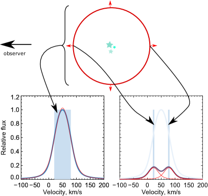
Figure 2: Schematic representation of the expanding shell (top) and examples of the emission-line profiles in its different parts (bottom). Bottom left: integrated emission-line profile of the shell, bottom right: line profile towards the center of the shell. The blue rectangle shows the model spectrum excluding thermal, turbulent, and instrumental broadening. The blue curve shows the line profile including thermal, turbulent, and instrumental broadening, the red line shows the one- or two-component Voigt profile fit.

Thus in the uniform bubble model considered the observed integrated line profile has a rectangular shape with the same radiation flux density $F_{v}(v)$ over the velocity interval $[v_{\rm sys}-v_{\rm exp};v_{\rm sys}+v_{\rm exp}]$ also in the absence of radiation outside this interval (see the left-hand panel in Fig. 2). In contrast, if only the central part of such an idealized model is observed, the emission line-profile has the form of two narrow rectangular peaks with velocities corresponding to the ray velocities of the approaching and receding sides of a bubble, and their difference is equal to $2\times v_{\rm exp}$ (see the right-hand panel in Fig. 2).

In the above scheme only the contribution of the bubble expansion to the line profile is taken into account, ignoring the thermal and natural broadening and the contribution of the turbulence of the interstellar medium. Let us consider these effects in the next section.

2.2 Estimating Thermal and Turbulent Line Broadening

The width of emission lines in the interstellar medium is influenced by three main factors: natural line broadening (due to quantum uncertainty of the level energy with a finite lifetime), thermal line broadening and gas turbulence. The contribution of natural line broadening in this case is negligible compared to other factors, so we will consider only the effect of the latter two factors.

Under the assumption of local thermodynamic equilibrium, the velocity of thermal motion of electrons in H II-regions is described by the Maxwell distribution, according to which the dispersion of the velocity projection is equal to

$$\sigma_{\rm{th}}=\sqrt{\dfrac{k_{B}T_{e}}{m}},$$ (4)

which corresponds to $\sigma_{\rm th}\sim 9.1$ km s^-1 for HII for the adopted characteristic electron temperature $T_{e}=10^{4}$ K (Osterbrock and Ferland, 2006)

The situation with estimating the velocity dispersion of turbulent motions in the interstellar medium is more complicated. Observations indicate supersonic velocity dispersion for turbulent motions of ionized gas in galaxies (Moiseev et al., 2015; Varidel et al., 2020), which may be due to gravitational instability combined with feedback from massive stars (Krumholz et al., 2018). The observed dispersion of ionized gas velocities in this case correlates with the star-formation rate in the galaxy, and the characteristic velocity dispersions in nearby dwarf galaxies are $\sigma_{\rm turb}\sim 12$–$35$ km s^-1 (Moiseev et al., 2015), although they can be several times greater for galaxies with high star-formation rates. With integral field spectroscopy data available this quantity can be estimated for each individual object under study, for example, as the flux-weighted average of the velocity dispersion of bright H II regions (Moiseev and Lozinskaya, 2012) in the H$\alpha$ line.

Thus because of thermal broadening and turbulent motions in the interstellar medium the observed emission lines originating from outside the shell have a Gaussian profile with velocity dispersion

$$\sigma_{\rm ISM}=\sqrt{\sigma_{\rm th}^{2}+\sigma_{\rm turb}^{2}}\sim 15\hbox{--}36~{}\text{km\,s${}^{-1}$}$$ (5)

Assuming that the above mechanisms produce the comparable broadening of the emission lines from the walls of a bubble and from the surrounding interstellar medium, the final line profile from the shell can be obtained by convolving the rectangular distribution obtained in the previous section with a Gaussian function with a width of $FWHM=2\sqrt{2\ln{2}}\,\sigma_{\rm ISM}$.

2.3 Comparison of Model and Observed Line Profiles

The observed shape and width of a spectral line depend on the instrumental profile of the spectrograph. The instrumental profile of the FPI in SCORPIO-2 is well described by the Lorentz function, which means that the final observed emission-line profile can be approximated by the Voigt function, which is a convolution of the Gaussian and Lorentz functions (Moiseev and Egorov, 2008). Fig. 2 shows that after thermal, turbulent, and instrumental broadening are taken into account, the line profile from the model considered is indeed similar to those observed with the FPI (see Section 4). The integrated line profile can be well described by a single-component Voigt function, and the line profile in the direction of the center of a bubble, by a two-component Voigt function with the components centered on the velocities of the approaching and the receding sides.

We now use the model constructed to illustrate how insufficient angular resolution can distort the estimate of the bubble expansion velocity determined by decomposing the observed profile into components. Fig. 3 shows examples of simulated shell line profiles (expanding with a velocity of $v_{\rm exp}=35$ km s^-1 in a medium with $\sigma_{\rm ISM}=15$ km s^-1 and observed with an IFP751 FPI having LSF width $FWHM_{\rm LOR}=18$ km s^-1) integrated over different apertures. The smallest aperture corresponds to the central part of the shell, and the largest, to the integrated spectrum from the entire region. While in the former case the line profile clearly breaks into two components, there is no such separation in the case of the integrated spectrum corresponding to the case of a completely unresolved shell. The separation between the individual components can be seen to decrease with increasing relative area of the aperture compared to the total area occupied by a bubble in the sky plane. In the case considered, the shell expansion velocity is underestimated by a factor of 1.5 for an aperture with 50% of the total bubble area. Thus even if spectroscopic resolution is sufficient to decompose the profile into kinematically distinct components, insufficient angular resolution may result in a significantly underestimated shell expansion velocity and hence overestimated kinematic age and underestimated energy inflow required for the formation of these components. To correctly determine these parameters the angular resolution of the data has to be 0.5 of the shell size or better. This imposes a significant limitation on the use of estimates obtained by line-profile decomposition for bubbles smaller than 100 pc in the case of observations of galaxies beyond the Local Group.

In addition to the decomposition of the observed profile into kinematically isolated components, there are a number of other methods for estimating the expansion velocities of nebulae from published observational data. Guerrero et al. (1998) suggested using radial gradient of the line profile width to compute the expansion velocities of nebulae. However, this method is not applicable in the case of insufficient angular resolution or nonuniform nebulae. Dewey (2010) described yet another method in his paper on the interpretation of the kinematics of unresolved young supernova remnants. Like in this paper (cf. Section 2.1), the above author assumes that the integrated spectrum of an expanding supernova remnant has a uniform distribution with velocities from $-v_{\rm exp}$ to $v_{\rm exp}$, but he ignores the effects due to turbulence in the surrounding interstellar medium (which is true in first approximation given that characteristic shock velocities in young supernova remnants are one to two orders of magnitude higher than those discussed in our paper) or the non Gaussian shape of the spectrograph instrument profile. Dewey computes the dispersion of the uniform distribution from $a$ to $b$ (from $-v_{\rm exp}$ to $v_{\rm exp}$) as

$$\sigma=\sqrt{\dfrac{(b-a)^{2}}{12}}=\sqrt{\dfrac{v_{exp}^{2}}{3}}\approx 0.577\ v_{\rm exp},$$ (6)

to determine the expansion velocity of supernova remnants from the observed line width. Note that this is not entirely correct, because the velocity dispersion estimated by fitting the distribution to a Gaussian function ($\sigma\approx 0.715\ v_{\rm exp}$) differs from that given above for the uniform distribution. With the above fact taken into account, the solution proposed by Dewey (2010) coincides with a special case of the method we consider below (see Section 3) in the case of zero turbulent motions in the interstellar medium.

Thus, simple approaches can yield significantly (by tens of percent) underestimated or overestimated results. Below we propose a method for estimating shell expansion velocities from the measured width of the integrated line profile based on modeling that takes into account the main effects described above that affect the observed shape of the profile.

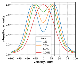
Figure 3: Model emission-line profile of a bubble expanding with velocity $v_{\rm exp}=35$ km s^-1 (marked with vertical lines) in the medium with $\sigma_{\rm ISM}=15$ km s^-1 and “observed” with spectrograph with Lorentzian LSF $FWHM_{\rm LOR}=18$ km s^-1. Different colors correspond to different apertures in the integration: 1% of the total area in the sky plane corresponds to the center of the bubble and 100%, to the entire shell.

3 MEASURING A BUBBLE EXPANSION VELOCITY BASED ON THE OBSERVED VELOCITY DISPERSION

As noted above, when the angular and/or spectral resolution of the employed is insufficient, the expansion of a bubble shows up as an increase in the measured velocity dispersion. This effect is often apparent in observations. Thus one can efficiently search for expanding superbubbles in nearby galaxies by analyzing ($I$–$\sigma$) diagrams in the H$\alpha$ line (Muñoz-Tuñón et al., 1996; Moiseev and Lozinskaya, 2012; Egorov et al., 2017, 2018, 2021), where such objects can be distinguished by their increased velocity dispersion. Compact nebulae around individual energetic objects (WR, LBV stars) and unresolved supernova remnants also stand out on the ($I$–$\sigma$)-diagram as regions with high intensity and high velocity dispersion (Moiseev and Lozinskaya, 2012). Below we investigate how to estimate the expansion velocities of such bubbles based on the data about the spatial distribution of velocity dispersion in their host galaxy.

To reveal the relationship pattern between the measured spectral line width and the actual shell expansion velocity, we constructed and analyzed a series of model spectra computed for the case of a uniform bubble expanding in turbulent interstellar medium (see Section 2). In our analysis we varied the shell expansion velocity and the velocity dispersion in the interstellar medium (which includes turbulent and thermal line broadening) in the intervals $v_{\rm exp}=5$–$95$ km s^-1 and $\sigma_{\rm ISM}=3$–$70$ km s^-1, respectively. As mentioned above (see Section 2.3), the instrumental profile of the FPI can be well described by the Lorentz function. At the same time, the LSF shape of classical integral field spectrographs have an LSF is close to Gaussian (e.g., MaNGA (Law et al., 2021), MUSE (Bacon et al., 2010), IFU within SCORPIO-2 (Afanasiev et al., 2018)). We considered four types of LSF in our analysis:

• 1) Gaussian LSF with the profile width $FWHM_{\rm LSF}$. In this case the effect of instrumental broadening on the integrated line profile is similar to that due to turbulent line broadening, so we consider the quantity $\sqrt{\sigma_{\rm ISM}^{2}+\sigma_{\rm LSF}^{2}}$, where $\sigma_{\rm LSF}=FWHM_{\rm LSF}/(2\sqrt{2\ln 2})$, as a parameter for further analysis. Here we estimate the “observable” velocity dispersion $\sigma_{\rm obs}$ measured from the integrated spectrum of the shell by fitting the line profile to a Gaussian function.

• 2) The case of the LSF in the form of a Lorentz function. In that case we set $\sigma_{\rm LSF}=0$ in all further computations. Note that here the measured velocity dispersion $\sigma_{\rm obs}$ inferred by fitting the observed profile to a Voigt function is free from the contribution of instrumental broadening, because it refers to the Gaussian component (Moiseev and Egorov, 2008). We considered three values of the Lorentzian profile width corresponding to the three FPIs used in SCORPIO-2 on the 6-m telescope of the SAO RAS:

  • $FWHM_{\rm LOR}=18$ km s^-1 (for IFP751);

  • $FWHM_{\rm LOR}=36$ km s^-1 (for IFP501);

  • $FWHM_{\rm LOR}=78$ km s^-1 (for IFP186).

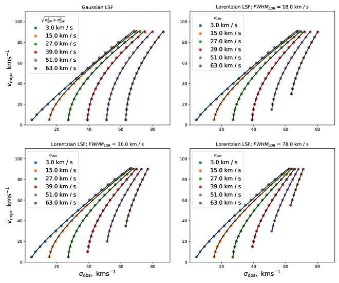
Figure 4: Relationship between the expansion velocity $v_{\rm exp}$, observed velocity dispersion $\sigma_{\rm obs}$, unperturbed interstellar medium velocity dispersion $\sigma_{\rm ISM}$, and the shape and width of the instrumental profile ($FWHM_{\rm LOR}$, $\sigma_{\rm LSF}$) as inferred in terms of the uniform expanding bubble model. The solid lines show the result of the best approximation by a relation of the form (7).

Fig. 4 shows the dependence of the model-estimated expansion velocity of a bubble on the velocity dispersion $\sigma_{\rm obs}$ measured from its integrated spectrum, for different values of $\sigma_{\rm ISM}$. For each of these, the resulting dependencies are well approximated by a relation of the form

$$v_{\rm exp}=k(\sigma_{\rm obs}^{2}-(\sigma_{\rm ISM}^{2}+\sigma_{\rm LSF}^{2}))^{a}+v_{0}.$$ (7)

The coefficients $k$, $v_{0}$ and exponent $a$ in the formula depend on the average dispersion of gas velocities in the galaxy $\sigma_{\rm ISM}$ as well as on the form and width of the instrumental profile of the spectrograph (parameters $\sigma_{\rm LSF}$ and $FWHM_{\rm LOR}$). Figure 5 shows the behavior of the dependence of each parameter on these quantities. Note that the parameter $v_{0}$ is relevant only in the case of high velocity dispersion $\sigma_{\rm ISM}$ of unperturbed gas and is most important in the case of the use of the low spectral resolution FPI, which is poorly suited to study gas velocity dispersion variations in galaxies. We can assume $v_{0}\simeq 0$ in most cases of typical velocity dispersions $\sigma_{\rm ISM}\sim 12$–$35$ km s^-1 in nearby galaxies (Moiseev, 2015).

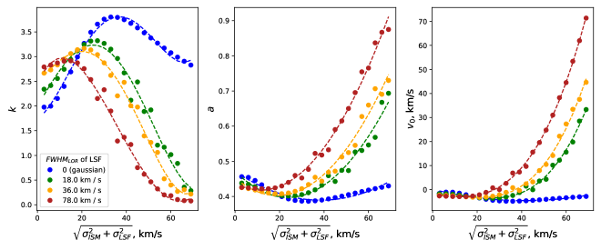
Figure 5: Dependence of parameters $k$, $a$ and $c$ in equation (7) on the shape and width of the instrumental spectrograph contour $\sigma_{\rm LSF}$, $FWHM_{\rm LOR}$ and on the average gas velocity dispersion $\sigma_{\rm ISM}$ in the galaxy. The dashed line shows the result of the best polynomial approximation according to the equations (8)–(10) and Table 1.

The variation of each of the parameters $k$, $a$, $v_{0}$ in formula (7) as a function of $\sqrt{\sigma_{\rm ISM}^{2}+\sigma_{\rm LSF}^{2}}$ can be described by the following polynomial relations

$$k(x) = c_{k4}x^{4}+c_{k3}x^{3}+c_{k2}x^{2}+c_{k1}x+c_{k0},$$ (8)

$$a(x) = c_{a2}x^{2}+c_{a1}x+c_{a0},$$ (9)

$$v_{0}(x) = c_{v3}x^{3}+c_{v2}x^{2}+c_{v1}x+c_{v0},$$ (10)

, where $x=\sqrt{\sigma_{\rm ISM}^{2}+\sigma_{\rm LSF}^{2}}$ ($\sigma_{\rm LSF}=0$ in the case of the Lorentz instrumental profile). The coefficients in equations (8)–(10) are listed in Table 1 for all the four LSF types considered.

Table 1: Polynomial expansion coefficients of parameters $k$, $a$ and $v_{0}$ according to equations (8)–(10) for different instrumental contour widths $FWHM_{\rm LOR}$

	$FWHM_{\rm LOR}$
Parameter	0 km s-1	18 km s-1	36 km s-1	78 km s-1
	(Gaussian LSF)	(IFP751)	(IFP501)	(IFP186)
$c_{k0}$	$1.74$	$2.0$	$2.49$	$2.45$
$c_{k1}$	$0.0257$	$0.0741$	$0.0433$	$0.102$
$c_{k2}$	$4.60e-03$	$4.29e-04$	$5.99e-04$	$-5.57e-03$
$c_{k3}$	$-1.42e-04$	$-7.34e-05$	$-7.62e-05$	$6.37e-05$
$c_{k4}$	$1.06e-06$	$6.75e-07$	$7.48e-07$	$-1.65e-07$
$c_{a0}$	$0.471$	$0.472$	$0.452$	$0.438$
$c_{a1}$	$-4.27e-03$	$-6.30e-03$	$-5.26e-03$	$-3.48e-03$
$c_{a2}$	$5.54e-05$	$1.33e-04$	$1.38e-04$	$1.50e-04$
$c_{v0}$	$0.139$	$-2.0$	$-2.17$	$-2.18$
$c_{v1}$	$-0.23$	$0.0922$	$0.0215$	$-0.091$
$c_{v2}$	$2.81e-03$	$-0.0128$	$-9.37e-03$	$-0.0011$
$c_{v3}$	$-3.18e-07$	$2.73e-04$	$2.78e-04$	$2.61e-04$

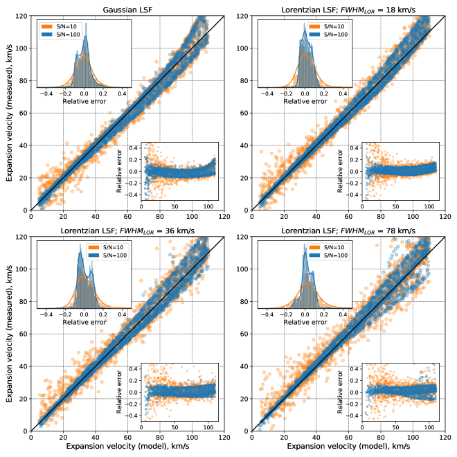
Figure 6: Dependence of uniform shell expansion velocity measured by the equations (7)–(10) on the input velocity given in the simulation. For each LSF type and width, model line profiles are generated for 4000 bubbles with $S/N=10$ (the orange symbols) and $S/N=100$ (the blue symbols), expansion velocity $v_{\rm exp}$ (5 to 110 km s^-1), ambient gas velocity dispersion $\sigma_{\rm ISM}$ (10 to 70 km s^-1, it includes the instrumental profile width in the case of Gaussian LSF). Panels for different LSF types and widths are presented. The histogram in each panel shows the distribution of the relative measurement error $(v_{\rm exp}[\mathrm{measured}]-v_{\rm exp}[\mathrm{model}])/v_{\rm exp}[\mathrm{model}]$. The bottom of each panel shows the distribution of the relative error on input $v_{\rm exp}$.

To estimate the relative error of the shell expansion velocity inferred from equation (7) and the robustness of the equations (7)–(10) with respect to noise, we performed an additional Monte Carlo simulation. For each of the four LSF types, we simulated 4000 spectra of bubbles with random parameters constrained in the intervals $\sqrt{\sigma_{\rm ISM}^{2}+\sigma_{\rm LSF}^{2}}=10$–$70$ km s^-1 and $v_{\rm exp}=5$–$110$ km s^-1, and added noise with final signal-to-noise ratios of $S/N=10$ and $S/N=100$. We applied equations (7)–(10) to the resulting synthetic profiles and estimated the bubble expansion velocity in each case. A comparison of the resulting estimate with its true value set in the model demonstrates the accuracy of the technique. Fig. 6 shows the dependence of these two quantities on each other as well as the distribution of the relative measurement error computed as $(v_{\rm exp}[\mathrm{measured}]-v_{\rm exp}[\mathrm{model}])/v_{\rm exp}[\mathrm{model}]$. As is evident from the figure, the technique described above is quite robust with respect to noise and the shell expansion velocity to be estimated with an accuracy of about 10% over a wide range of velocities.

The method described above is based on the uniform bubble model, but real H II regions have a more complex morphology. First, the observed superbubbles in extragalactic star-forming regions form as a result of energy inflow from multiple massive stars, i.e., in fact, they are complexes of merging local bubbles at different stages of evolution. As was shown by Tenorio-Tagle et al. (1996), the integrated spectrum of such unresolved complexes ca still be well described by the model of a single uniform superbubble, but there may be an additional broad low-intensity component in the line wings—its contribution does not affect the analysis considered in this paper. The second important point is that real H II regions are not uniform but highly clumped with significant local density and temperature inhomogeneities. Let us check to what extent this effect affects our estimates.

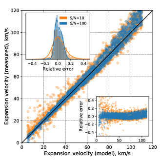
Figure 7: Same as in Fig. 6, but for the models of bubbles with nonuniform brightness distribution. The dependences are shown only for the LSF in the form of a Lorentz function with profile width $FWHM_{\rm LOR}=18$ km s^-1.

We now consider a shell in the form of a thin expanding sphere, but this time the brightness of each element $dV$ in Fig. 1 varies with angles $\theta$ and $\varphi$. For this purpose, we set the distribution $I(\theta,\varphi)$ in the form of the sum of spherical harmonics up to and including the eighth order with random amplitudes and with the dominant contribution of the angle-independent (zero) component. The final intensity distribution from each element in the bubble is a set of separate spots of various sizes with higher- and lower-than average brightness. As in the case of the uniform model, the integrated spectrum of the resulting shell is convolved with a Gaussian to account for thermal and turbulent broadening and with a Gaussian or Lorentz function describing the instrumental profile of the spectrograph. To test the applicability of equations (7)–(10) to such structures with non-uniform brightness distributions, we performed Monte Carlo simulations similar to those described above, but this time with synthetic profile generated in terms of a nonuniform bubble model. Fig. 7 shows the result of comparing the measured and modeled bubble expansion velocities (for $FWHM_{\rm LOR}=18$ km s^-1). The number of regions exhibiting a significant deviation of the result from the model is slightly higher than in the case of a uniform shell, but on the average the relative error is still at the level of about 10%. Hence the method described is also applicable in the case of shell structures with nonuniform brightness distribution.

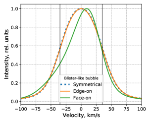
Figure 8: Integrated model line profile from an expanding spherical bubble (the blue line) in the form of a hemisphere at different orientations. In the case where the bright part of the bubble is in the sky plane (the green line), the resulting integrated profile is significantly asymmetric. When the bright part of the bubble is perpendicular to the sky plane (the orange line) the resulting line profile is indistinguishable from the case of spherical symmetry. The vertical lines correspond to the preset expansion velocity $v_{\rm exp}=35$ km s^-1.

In the cases where star formation occurs at the boundary of a molecular cloud, significant gas density gradient of gas density around massive stars can cause the formation of asymmetric shells with azimuthal gradient of brightness and velocity. Typical examples are blister-type nebulae (see, e.g., Egorov et al. (2010)). To test the applicability of the above technique to such objects, we simulated a shell structure with smooth azimuthal variation of brightness and velocity. Given that the brightness of the emission-line nebula depends on gas density $I\sim n_{e}^{2}\sim\rho^{2}$ (Osterbrock and Ferland, 2006), and that relation $v\rho^{2}\sim const$ (McKee and Cowie, 1975) is usually fulfilled for radiative shocks, we can specify the expansion velocity of our asymmetric shell at each point by the law $v\sim I^{-1}$. From observational point of view we can distinguish two extreme cases: the bright (dense) side of the shell is in the sky plane (face-on) or perpendicular to it (edge-on). In the first case such a shell appears as an ordinary symmetric H II region, whereas in the second case there should be clear brightness gradient (in the case of sufficient angular resolution). Fig. 8 shows the simulated integrated profiles for each of these cases. As is evident from the figure, the integrated line profile of a blister-type profile is indistinguishable from the spherically symmetric case in its edge-on orientation, and hence the method we have described above is fully applicable to such objects. On the other hand, in the case of face-on orientation the integrated profile is significantly asymmetric, resulting in underestimated measured velocity dispersion and, consequently, underestimated bubble expansion velocity. Thus, in the case shown in Fig. 8, a formal fit of the asymmetric face-on profile of the shell by a single-component Voigt function and application of equations (7)–(10) yields an expansion velocity estimate of $v_{\rm exp}=30$ km s^-1 instead of 35 km s^-1 value incorporated into the model, and the discrepancy is significantly greater in the case of higher expansion velocities. Unfortunately, even in the case of sufficiently high angular resolution distinguishing such face-on blister-type nebulae from spherically symmetric ones is by no means a trivial task. In this connection, it is worth noting that the method presented in this paper may be unreliable in cases where the integrated line profile of a nebula is significantly asymmetric.

The method described in this section allows us to use equations (7)–(10) to determine the expansion velocities of spatially unresolved (or poorly resolved) bubbles in the interstellar medium of galaxies based on the gas velocity dispersion $\sigma_{\rm obs}$ measured from the integrated spectrum of a bubble and the average gas velocity dispersion in the galaxy $\sigma_{\rm ISM}$. The gas velocity dispersion $\sigma_{\rm ISM}$ in this case can be inferred, for example, from the estimated flux-weighted average gas velocity dispersion of the bright H II regions in the galaxy, which stand out in the ($I$–$\sigma$) diagrams. The presented method can also be useful in the case of spatially resolved shell structures when insufficient spectral resolution prevents the decomposition of the profile into kinematically isolated components. In the next section we test the method on real observational data.

4 THE GALAXY IC 1613: TESTING THE METHOD ON OBSERVATIONAL DATA

Nearby star-forming dwarf galaxies are an excellent laboratory for studying the interaction processes of massive stars and the interstellar medium. Because of the lack of spiral density waves and the thick gaseous disk extended supershell complexes are often observed in the interstellar medium of such galaxies. Such a pattern can be clearly seen in IC 1613—a nearby Local Group galaxy (at a distance of $D\sim 760$ kpc (Karachentsev et al., 2013). A complex of expanding superbubbles of ionized gas extending over about 1 kpc is observed in its eastern part (see Fig. 9). This complex of superbubbles has been studied in detail previously by Lozinskaya et al. (2003) and is well suited for testing the method described in Section 3 on real data.

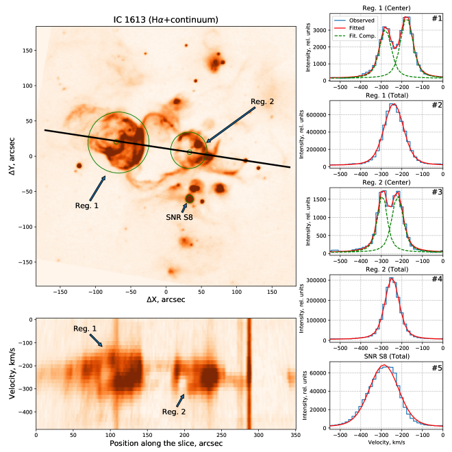
Figure 9: Complex of superbubbles in the galaxy IC 1613 according to H$\alpha$-line SCORPIO observations on the 6-m telescope of the SAO RAS. Top left panel: H$\alpha$-line image of the region, the position of the cut (the black line) for the “position-velocity” diagram (shown in the bottom left panel). The right panel shows the observed H$\alpha$-line profiles by integration in the apertures shown by the green circles in the image. The profiles #1, #3 are obtained for the central part of the considered regions, and profiles #2, #4—for the entire region. Profile #5 corresponds to the bubble surrounding the young SNR S8 supernova remnant. The dashed green line shows the individual components, and the red line, the final fit of the observed profile by a one- or two-component Voigt function.

We use H$\alpha$-line data obtained on September 13, 2001 with the FPI (IFP501) of the SCORPIO focal reducer (Afanasiev and Moiseev, 2005) mounted on the BTA 6-m telescope of the SAO RAS. For a detailed description of the observations and data processing see Lozinskaya et al. (2003).

As is evident from Fig. 9, the two regions labeled Reg. 1 and Reg. 2 exhibit a clear shell-like morphology and reveal a characteristic velocity ellipse in the “position-velocity” diagrams, indicating the observed superbubble expansion. The angular size of these superbubbles is on the order of $80\arcsec$ and $55\arcsec$ (290 and 200 pc), respectively, which significantly exceeds the angular resolution of the observational data (about $1.5\arcsec$). The observed H$\alpha$ profile in the central part of the shells (#1 and #3 in Fig. 9) is clearly separated into components corresponding to the approaching and the receding sides. The expansion velocities of the Reg. 1 and Reg. 2 shells computed from the maximum separation of the H$\alpha$ profile components are equal to $v_{\rm exp}=51$ km s^-1 and 37 km s^-1 respectively.

Superbubbles similar to Reg. 1 and Reg. 2 observed in more distant galaxies will have smaller angular sizes, and they should be practically unresolvable at $D\sim 10$ Mpc. In such a case their integrated spectrum will be observed, as in the case of profiles #2 and #4 in Fig. 9. No separation into individual components can be observed, but the H$\alpha$ profile is broadened. The measured velocity dispersion (free of instrumental broadening) is $\sigma_{\rm obs}=39$ km s^-1 and 26 km s^-1 for Reg. 1 and Reg. 2, respectively. We can estimate the velocity dispersion of the surrounding interstellar medium as the flux-weighted average H$\alpha$-line velocity dispersion in regions with intensities higher than the median I (H$\alpha$) in the galaxy (to exclude the contribution of diffuse ionized gas). The inferred velocity dispersion $\sigma_{\rm ISM}=15$ km s^-1 is consistent with the estimate of the velocity dispersion of individual components on the profile #3, as well as with an estimate for separate bright H II regions, which exhibit no signs of expansion. We can adopt these values $\sigma_{\rm ISM}$ and $\sigma_{\rm obs}$ and $FWHM_{\rm LOR}=36$  km s^-1 for IFP501 and use equations (7)–(10) to estimate expansion velocity by the method proposed in this paper. The inferred expansion velocity estimates $v_{\rm exp}=53$ km s^-1 and 33 km s^-1 for Reg. 1 and Reg. 2, respectively, agree well with those found above, which are based on the H$\alpha$-line profile decomposition within the previously quoted relative error of the method (on the order of 10%).

The only known supernova remnant in the IC 1613 galaxy—SNR S8—is also observed toward the complex considered, but, unlike Reg. 1 and Reg. 2 regions, it is practically unresolved, making it impossible to directly measure directly its expansion velocity. Observational data obtained with MPFS spectrograph attached at the 6-m telescope of the SAO RAS Lozinskaya et al. (1998) revealed no velocity dispersion gradient that could clearly indicate SNR expansion, and yielded a rough estimate $v_{\rm exp}\sim 50$–$100$ km s^-1 based on the variation of the observed radial velocity toward the SNR ($v_{\rm exp}<300$ km s^-1 if weak emission structures are also considered). A detailed study of SNR S8 is also given in Schlegel et al. (2019). Direct measurements of the expansion velocity of the supernova remnant are still lacking, but new high-resolution X-ray data have allowed the authors to estimate SNR S8 properties, including its age, independent of kinematic parameters.

We now try to estimate the expansion velocity of SNR S8 and its kinematic age from available observational data obtained with the FPI using equations (7)–(10). The integrated profile in the H$\alpha$ line (#5 in Fig. 9) is significantly broadened and slightly asymmetric. The measured velocity dispersion $\sigma_{\rm obs}=64$ km s^-1 corresponds to the optical shell expansion velocity $v_{\rm exp}=84$ km s^-1, which agrees with the approximate estimate obtained in Lozinskaya et al. (1998). The velocity thus measured corresponds to the velocity of the radiative shock propagating in regions of increased supernova remnant density, while the shock velocity outside dense clouds, which determines the remnant expansion velocity, is related to the gas density as (McKee and Cowie, 1975): $\beta n_{i}v_{s}^{2}=n_{c}v_{c}^{2}$, where $\beta=3.15$ for fast shocks, $n_{i}$ and $n_{c}$ are equal to the gas density in unperturbed interstellar medium and in a dense cloud, respectively; $v_{s}$ is the SNR shock front velocity in unperturbed medium, $v_{c}$—radiative shock velocity in a dense cloud. When applied to SNR S8 $v_{c}=v_{\rm exp}\simeq 84$ km s^-1, $n_{i}\simeq 1.6$ cm^-3 (according to Schlegel et al. (2019)), $n_{c}=n_{e}/1.2\simeq 1080$ (according to electron density estimate $n_{e}$ obtained by Lozinskaya et al. (1998) by the [S II] 6717/6731 Å lines ratio). From this, we find the velocity of the shock front SNR S8 $v_{s}\simeq 1230$ km s^-1. Assuming that SNR S8 is at the adiabatic stage of expansion (similar to Schlegel et al. (2019)), we can describe its evolution as $R_{s}\sim t^{0.4}$ (Sedov, 1959), which means that $t=0.4R_{s}/v_{s}$. Taking the estimate $R_{s}\sim 9.5$ pc obtained in Schlegel et al. (2019) from X-ray images, we determine the kinematic age value of SNR S8 $t\simeq 3100$ years, which agrees well with the independent estimate $t\simeq 3380$–$5650$ years obtained in Schlegel et al. (2019) who did not use an information on the gas kinematics.

We thus used the IC 1613 galaxy as an example to demonstrate that the method for measuring a bubble/superbubble expansion velocity described in this paper is applicable to real observational data and yields the expansion velocity and age estimates that are consistent with other independent measurements.

5 SUMMARY

Integral field spectroscopy reveals variations of the observed gas velocity dispersion in galaxies that are driven by presence of the expanding bubbles and superbubbles surrounding massive stars and clusters in star-forming regions (see, e. g., Moiseev and Lozinskaya, 2012). With high enough spectral resolution the observed emission line profile in such regions can be decomposed into kinematically isolated components allowing the bubble expansion velocity to be measured (see, e.g., Lozinskaya et al. (2003); Egorov et al. (2014, 2017); Oparin et al. (2020)), but this is rarely possible for galaxies located beyond the Local Group because of limited spatial resolution. In this paper, we propose a method allowing one to overcome this limitation and estimate the shell expansion velocity from the dispersion of gas velocities measured from integrated spectrum.

We considered an analytical model of a uniform thin shell expanding in a turbulized interstellar medium and found how thermal, turbulent, and instrumental broadening and bubble expansion affect the shape of the observed emission line profile. We used this model to demonstrate that the shell expansion velocity obtained by decomposing the profile into kinematically separated components can be significantly underestimated if the angular resolution is insufficient. This results in overestimated kinematic age and underestimated energy inflow required for the formation of the shell, and these biases can affect the estimated efficiency of the transfer of energy from stars to kinetic energy of superbubbles when comparing observations and theoretical models.

The models we have built showed that the bubble expansion velocity can be determined by equation (7), which includes the gas velocity dispersion of the bubble (measured from the integrated spectrum) and in the surrounding unperturbed interstellar medium (which can be estimated for each galaxy as a flux-weighted average value for bright H II regions). We showed that the parameters used in equation (7) depend on the average gas velocity dispersion in the galaxy and can be approximated by polynomials (8)–(10). The coefficients in these polynomials depend on the type of instrumental profile of the spectrograph. We considered the cases of LSF in the form of Gaussian functions (applicable to most classical integral field spectrographs) with arbitrary spectral resolution and Lorentz functions (for FPI) with the resolution corresponding to IFP751, IFP501, and IFP186, which are used in SCORPIO-2 instrument at the 6-m telescope of the SAO RAS. Table 1 lists the coefficients inferred for these cases.

We applied the method described to synthetic spectra of bubbles having random parameters and different $S/N$ ratios in their spectra and showed that the relative error of the measurement of the bubble expansion velocity is on average about 10%. To further test the applicability of the method, we also analyzed a bubble model with a non-uniform brightness distribution and found the result to be the same. We showed that the method is also applicable to bubbles with large-scale inhomogeneities (for example, those having the form of a hemisphere), but in this case, the spatial orientation of bright regions plays an important role.

We used the method described to estimate the expansion velocities of well-resolved shells of ionized gas and of the only known supernova remnant (SNR S8) in the nearby galaxy IC 1613. The estimates obtained for the superbubbles agree well with measurements made by decomposing the line profile into kinematically separated components. For the first time we estimated the kinematic age of SNR S8 ($t\simeq 3100$ years) and our result agrees well with the age obtained earlier from X-ray data (Schlegel et al., 2019).

The method proposed in this paper allows measuring the expansion velocities of spatially unresolved (or poorly resolved) superbubbles in galaxies outside the Local Group. In particular, it is intended to be used to measure the expansion velocities, kinematic ages, and energy of superbubbles identified by increased gas velocity dispersion from observations of nearby dwarf galaxies with a FPI at the 6-m telescope of the SAO RAS within the framework of SIGMA-FPI catalog. (Egorov et al., in prep.).

FUNDING

This work was supported by the Russian Science Foundation (Grant No. 19-72-00149). Observations on the 6-m telescope of the Special Astrophysical Observatory of the Russian Academy of Sciences are supported by the Ministry of Science and Higher Education of the Russian Federation (contract No. 05.619.21.0016, project identifier RFMEFI61919X0016). The renovation of telescope equipment is currently provided within the national project ”Science.”

CONFLICT OF INTEREST

The authors declare that there is no conflict of interest.

Translated by A. Dambis

References

- Afanasiev and Moiseev (2005) V. L. Afanasiev and A. V. Moiseev, \alet31, 194 (2005).
- Afanasiev and Moiseev (2011) V. L. Afanasiev and A. V. Moiseev, Baltic Astronomy 20, 363 (2011).
- Afanasiev et al. (2018) V. L. Afanasiev, O. V. Egorov, and A. E. Perepelitsyn, \ab73, 373 (2018).
- Bacon et al. (2010) R. Bacon, M. Accardo, L. Adjali, et al., Proc. SPIE7735, 773508 (2010).
- Bagetakos et al. (2011) I. Bagetakos, E. Brinks, F. Walter, et al., AJ141, 23 (2011).
- Churchwell et al. (2006) E. Churchwell, M. S. Povich, D. Allen, et al., ApJ649, 759 (2006).
- Dewey (2010) D. Dewey, Space Sci. Rev. 157, 229 (2010).
- Egorov et al. (2010) O. V. Egorov, T. A. Lozinskaya, and A. V. Moiseev, \arep54, 277 (2010).
- Egorov et al. (2014) O. V. Egorov, T. A. Lozinskaya, A. V. Moiseev, and G. V. Smirnov-Pinchukov, MNRAS444, 376 (2014).
- Egorov et al. (2017) O. V. Egorov, T. A. Lozinskaya, A. V. Moiseev, and Y. A. Shchekinov, MNRAS464, 1833 (2017).
- Egorov et al. (2018) O. V. Egorov, T. A. Lozinskaya, A. V. Moiseev, and G. V. Smirnov-Pinchukov, MNRAS478, 3386 (2018).
- Egorov et al. (2021) O. V. Egorov, T. A. Lozinskaya, K. I. Vasiliev, et al., MNRAS, 508, 2650 (2021).
- El-Badry et al. (2019) K. El-Badry, E. C. Ostriker, C.-G. Kim, et al., MNRAS490, 1961 (2019).
- Guerrero et al. (1998) M. A. Guerrero, E. Villaver, and A. Manchado, ApJ507, 889 (1998).
- Karachentsev et al. (2013) I. D. Karachentsev, D. I. Makarov, and E. I. Kaisina, AJ145, 101 (2013).
- Krumholz et al. (2018) M. R. Krumholz, B. Burkhart, J. C. Forbes, and R. M. Crocker, MNRAS477, 2716 (2018).
- Law et al. (2021) D. R. Law, K. B. Westfall, M. A. Bershady, et al., AJ161, 52 (2021).
- Lozinskaya (1992) T. A. Lozinskaya, Supernovae and stellar wind in the interstellar medium (Amer. Inst. of Physics, New York, 1992).
- Lozinskaya et al. (2003) T. A. Lozinskaya, A. V. Moiseev, and N. Y. Podorvanyuk, \alet29, 77 (2003).
- Lozinskaya et al. (1998) T. A. Lozinskaya, O. K. Silchenko, D. J. Helfand, and W. M. Goss, AJ116, 2328 (1998).
- Mac Low and McCray (1988) M.-M. Mac Low and R. McCray, ApJ324, 776 (1988).
- McKee and Cowie (1975) C. F. McKee and L. L. Cowie, ApJ195, 715 (1975).
- McLeod et al. (2019) A. F. McLeod, J. E. Dale, C. J. Evans, et al., MNRAS486, 5263 (2019).
- McLeod et al. (2020) A. F. McLeod, J. M. D. Kruijssen, D. R. Weisz, et al., ApJ891, 25 (2020).
- Moiseev (2015) A. V. Moiseev, \ab70, 494 (2015).
- Moiseev and Egorov (2008) A. V. Moiseev and O. V. Egorov, \ab63, 181 (2008).
- Moiseev and Lozinskaya (2012) A. V. Moiseev and T. A. Lozinskaya, MNRAS423, 1831 (2012).
- Moiseev et al. (2015) A. V. Moiseev, A. V. Tikhonov, and A. Klypin, MNRAS449, 3568 (2015).
- Moiseev et al. (2021) A. V. Moiseev, \ab76, 316 (2021).
- Muñoz-Tuñón et al. (1996) C. Muñoz-Tuñón, G. Tenorio-Tagle, H. O. Castañeda, and R. Terlevich, AJ112, 1636 (1996).
- Nath et al. (2020) B. B. Nath, P. Das, and M. S. Oey, MNRAS493, 1034 (2020).
- Oey (1996) M. S. Oey, ApJ467, 666 (1996).
- Oey and Clarke (1997) M. S. Oey and C. J. Clarke, MNRAS289, 570 (1997).
- Oey and García-Segura (2004) M. S. Oey and G. García-Segura, ApJ613, 302 (2004).
- Oparin et al. (2020) D. V. Oparin, O. V. Egorov, and A. V. Moiseev, \ab75, 361 (2020).
- Osterbrock and Ferland (2006) Astrophysics of gaseous nebulae and active galactic nuclei, 2nd ed., Ed.by D. E. Osterbrock and G. J. Ferland (University Science Books, 2006).
- Ramachandran et al. (2019) V. Ramachandran, W. R. Hamann, L. M. Oskinova, et al., \aaa625, id. A104 (2019).
- Schlegel et al. (2019) E. M. Schlegel, T. G. Pannuti, T. Lozinskaya, et al., AJ158, 137 (2019).
- Sedov (1959) L. I. Sedov, Similarity and Dimensional Methods in Mechanics (Academic Press, New York,1959).
- Sharma et al. (2014) P. Sharma, A. Roy, B. B. Nath, and Y. Shchekinov, MNRAS443, 3463 (2014).
- Tenorio-Tagle et al. (1996) G. Tenorio-Tagle, C. Munoz-Tunon, and R. Cid-Fernandes, ApJ456, 264 (1996).
- Varidel et al. (2020) M. R. Varidel, S. M. Croom, G. F. Lewis, et al., MNRAS495, 2265 (2020).
- Vasiliev et al. (2015b) E. O. Vasiliev, A. V. Moiseev, and Y. A. Shchekinov, Baltic Astronomy 24, 213 (2015b).
- Vasiliev et al. (2015a) E. O. Vasiliev, B. B. Nath, and Y. Shchekinov, MNRAS446, 1703 (2015a).
- Warren et al. (2011) S. R. Warren, D. R. Weisz, E. D. Skillman, et al., ApJ738, 10 (2011).
- Weaver et al. (1977) R. Weaver, R. McCray, J. Castor, et al., ApJ218, 377 (1977).
- Weisz et al. (2009) D. R. Weisz, E. D. Skillman, J. M. Cannon, et al., ApJ704, 1538 (2009).
- Yadav et al. (2017) N. Yadav, D. Mukherjee, P. Sharma, and B. B. Nath, MNRAS465, 1720 (2017).