Large-Scale Hyperspectral Image Clustering Using Contrastive Learning

Abstract

Clustering of hyperspectral images is a fundamental but challenging task. The recent development of hyperspectral image clustering has evolved from shallow models to deep and achieved promising results in many benchmark datasets. However, their poor scalability, robustness, and generalization ability, mainly resulting from their offline clustering scenarios, greatly limit their application to large-scale hyperspectral data. To circumvent these problems, we present a scalable deep online clustering model, named Spectral-Spatial Contrastive Clustering (SSCC), based on self-supervised learning. Specifically, we exploit a symmetric twin neural network comprised of a projection head with a dimensionality of the cluster number to conduct dual contrastive learning from a spectral-spatial augmentation pool. We define the objective function by implicitly encouraging within-cluster similarity and reducing between-cluster redundancy. The resulting approach is trained in an end-to-end fashion by batch-wise optimization, making it robust in large-scale data and resulting in good generalization ability for unseen data. Extensive experiments on three hyperspectral image benchmarks demonstrate the effectiveness of our approach and show that we advance the state-of-the-art approaches by large margins.

I Introduction

Recent advances in the Earth observation (EO) technology have provided end users with a large volume of remote sensing data comprised of rich spectral, spatial, and temporal information [1, 2]. As one of the most important technologies in EO, hyperspectral imaging has facilitated numerous promising applications in areas ranging from ocean, urban, agriculture, geology [3], to biomedicine [4], due to its unique advantages. Hyperspectral imagery (HSI) is characterized by hundreds of narrow spectral bands with a nanometer resolution, allowing more fine-grained recognition for objects of interest.

HSI intelligent interpretation has drawn increasing attention in recent years, wherein pixel-wise HSI classification lays a foundation for decision-making. Parallel to the development of supervised learning, supervised HSI classification has been extensively studied [5] over the last decade. Despite the observable advances, supervised methods commonly rely on sufficient training data. In particular, with the growing success of deep learning in HSI processing [6, 7], there is an increasing demand for large-scale training data paired with human annotations [8]. However, data annotation often requires considerable manpower and resources, as well as expert knowledge. This has become a severe bottleneck that restricts the development of HSI intelligent interpretation.

In contrast, there is a distinct gap between HSI clustering (i.e., unsupervised HSI classification) and supervised HSI classification [9]. Due to the absence of supervisory signals and also the ubiquitous spectral variability [10], HSI clustering is much more challenging than supervised tasks. The core of HSI clustering is to model the intrinsic interrelation between data points and clusters. Therefore, HSI clustering often involves pair-wise measurement criteria. For example, classic $k$-means [11] and fuzzy $c$-means [12] seek to find a set of cluster centers by calculating pair-wise distance. Instead, subspace clustering, e.g., sparse subspace clustering (SSC) [13] and low-rank subspace clustering (LRSC) [14], aims to learn the self-expressiveness of data. Beneficial from the good theoretical guarantees and robustness, subspace clustering has been widely applied for HSI clustering [9, 15, 16]. Despite their promising results, most of HSI clustering methods typically suffer from two drawbacks.

First, previous methods usually model in either raw feature space or hand-crafted feature space. This would produce inferior results on complex and high-dimensional HSI datasets caused by insufficient representability. To overcome the limitation, many efforts [17, 18, 19, 20] have been devoted to developing deep clustering models. The common idea is to incorporate a clustering objective function, often derived from classical clustering mechanisms with a proper relaxation, into a deep learning model and then jointly train for discriminative representations [21, 22]. For instance, deep subspace clustering networks (DSC) [23] and its variants [24, 9, 25] recast subspace learning into a latent self-expression layer of an autoencoder (AE). Similarly, soft and regularized $k$-means objective [26] is frequently adopted in learning clustering-friendly discriminative representations. This results in a series of state-of-the-art deep clustering models including deep embedded clustering (DEC) [27] and deep clustering network (DCN) [28]. However, the training schedule alternating between feature clustering and network parameters update leads to unstable learning of feature representations [29, 30].

Second, most of the existing HSI clustering methods belong to offline clustering models, resulting in two inevitable issues: poor scalability and generalization ability. However, these two properties are crucial for large-scale HSI clustering and application in industrial scenarios. Many attempts have been dedicated to addressing these limitations. For scalability, they presented some useful solutions from either data perspective, e.g., dimensionality reduction [31, 32] and superpixel segmentation [33], or model mechanism perspective including anchor graph [34] and sampling [35, 36, 37]. Whereas, there are fewer studies that have focused on the generalization ability of clustering models, especially in the HSI area. This is because most clustering methods can only handle offline tasks, i.e., the clustering is based on the whole dataset, leading to difficulty in dealing with unseen data. Moreover, pure unsupervised training for clustering may produce trivial solutions.

Recently, self-supervised learning [38] typified by contrastive learning [39, 40] has emerged as a powerful paradigm for representation learning. It also opens up a new path to smoothly overcome the aforementioned shortcomings. Based on the philosophy of “label is representation” [30, 41, 42], the pioneer of using contrastive learning for clustering, i.e., contrastive clustering (CC) [30], has shown state-of-the-art results in image clustering tasks. The approach conducts clustering through both instance-level and cluster-level contrastive learning, thereby avoiding explicit clustering objectives and resulting in remarkable flexibility on training and applying.

In this paper, we develop a one-stage online deep clustering approach for large-scale HSIs, termed as Spectral-Spatial Contrastive Clustering (SSCC), which recasts the clustering task into a self-supervised learning problem. The intuition behind the clustering model is based on an observation that a neural network always tends to activate the same neurons if the patterns belong to the same clusters. This signifies that the outputs of a softmax projection head with a dimensionality of the cluster number can naturally treat as soft pseudo labels. Following with this observation and the pioneer CC [30] approach, we present a new contrastive clustering framework based on exploiting twin neural networks to implicitly maximize within-cluster similarity and reduce between-cluster redundancy from a batch of distorted views augmented according to spectral and spatial properties. Unlike the CC approach that adopts dual InfoNCE [43] objectives and two asymmetric projection heads, our model is entirely symmetric containing only one projection head and includes a different objective based on the redundancy reduction suggested in Barlow Twins [40]. This alleviates the reliance on large batches and the risk of collapsed representations.

To summarize, our contributions are threefold:

• We propose SSCC approach for large-scale HSI clustering by using a self-supervised learning framework to learn discriminative label representations. The approach can be easily trained in an entirely end-to-end fashion by batch-wise optimization, making it scalable for large-scale HSIs and easy to generalize to unseen data. Instead of using dual projection heads and asymmetrical networks, we show that a single projection head with a symmetry architecture can produce better results.

• We introduce a novel objective function by leveraging both InfoNCE and Barlow Twins objectives, which implicitly encourage within-cluster similarity and between-cluster dissimilarity, respectively. To fully explore spectral and spatial information, we provide a semantic-preserving augmentation pool by distorting along both spectral and spatial dimensions.

• We systematically evaluate our approach on three HSI benchmarks, demonstrating that SSCC consistently outperforms the state-of-the-art approaches by large margins. We also show that SSCC indeed learns fine-grained semantic differences from our designed self-supervised task. The successful attempt provides an effective tool to narrow the gap between supervised and unsupervised learning.

The rest of this paper is structured as follows. First, we briefly review the related concepts, e.g., contrastive learning and HSI clustering methods, in Section II. Second, we describe the details of the developed SSCC approach in Section III. In Section IV, we provide systematic experimental results and analysis for our approach. Finally, we conclude with a summary and future works in Section V.

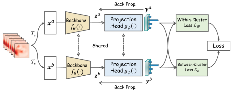
Figure 1: Overview of SSCC. Given a HSI cell $\boldsymbol{x}$ sampled from an HSI, we feed it into an augmentation pool $\mathcal{T}$ twice to generate two distorted views $\boldsymbol{x}^{a}$ and $\boldsymbol{x}^{b}$. Then, we forward them into a network twin consisting of a backbone $f_{\theta}\left(\cdot\right)$ followed by a projection head $g_{\phi}\left(\cdot\right)$ with $C$ softmax output neurons to obtain a pair of corresponding latent representations (i.e., $\boldsymbol{z}^{a}$ and $\boldsymbol{z}^{b}$) and label representations (i.e., $\boldsymbol{y}^{a}$ and $\boldsymbol{y}^{b}$). SSCC is trained in an end-to-end manner by optimizing an objective that uses $\mathcal{L}_{\mathcal{W}}$ to maximize within-cluster similarity and $\mathcal{L}_{\mathcal{B}}$ to minimize between-cluster correlation. During the inference stage, SSCC assigns label by taking the maximum activation of the label representations, making it robust to large-scale data and unseen data.

II Related Work

II-A Self-supervised Contrastive Learning

Self-supervised learning [38], as a subset of unsupervised learning, has emerged as a promising paradigm for representation learning. The goal of the paradigm is to learn general feature representation from large-scale unlabeled data without using any human-annotated labels. The pipeline of self-supervised learning can be broadly summarized into two steps. First, it trains a neural network to solve a predefined pretext task, such as predicting image rotations [44] and clustering labels [45]. Second, the pre-trained model is transferred to a specific downstream task, e.g., classification, segmentation, and object detection [39, 40, 44], by fine-tuning. On the basis of objectives, self-supervised learning can summarize into three categories [46]: generative, contrastive, and adversarial.

Due to the remarkable representation ability, self-supervised contrastive learning has attracted increasing interest [46]. Typically, the method involves data augmentations and twin network architectures (e.g., SimCLR [39]), while its objective frequently adopts InfoNCE [43] defined upon positive and negative pairs. Consequently, contrastive learning usually requires sufficient batch samples to prevent trivial solutions. To address the problem, momentum contrast (MoCo) suggests using a memory bank and momentum update mechanism. Recent efforts including bootstrap your own latent (BYOL) [47] and simple siamese (SimSiam) [48] show that asymmetric architecture and a mechanism called ’stop-gradient’ are probably the key factors of avoiding negative samples and collapsed representations. In Barlow Twins [40] approach, Jure et al. further simplified the training of contrastive learning by a symmetric architecture and an innovative redundancy reduction loss function.

Increasing evidence suggests that self-supervised learning has tremendous potential to break the dependencies on human-annotated labels. In the HSI area, self-supervised learning has achieved promising results across imaging [49], unmixing [50], and classification [51]. These indicate that the use of self-supervised learning for HSI clustering would make great sense for narrowing the gap between unsupervised learning and supervised learning of HSI.

II-B Deep Clustering

Unlike traditional clustering approaches, e.g., $k$-means [11], deep clustering refers to the clustering model based on deep learning, wherein deep learning is used to learn high-level features. Nonetheless, traditional clustering models are usually reformulated as a clustering regularization in the deep clustering [21]. A typical deep clustering objective can be expressed as $\mathcal{L}=\mathcal{L}_{clu}+\gamma\mathcal{L}_{rep}$, where $\mathcal{L}_{clu}$ and $\mathcal{L}_{rep}$ indicate a clustering loss and a representation loss, respectively. Taking DSC [23] as an example, $\mathcal{L}_{clu}$ is implemented by self-representation in a latent space and $\mathcal{L}_{rep}$ is a reconstruction error of AE.

The training of deep clustering may involve two stages or one stage. For the two-stage models like DeepCluster [45], they conduct network parameters update and feature clustering alternately. Despite their flexibility, these models often suffer from poor stability in clustering results and feature representation [29]. In contrast, one-stage models pursue clustering-friendly feature representation by jointly feature learning and clustering, significantly improving the clustering accuracy. Two representative instances of the one-stage model are DEC [27] and DSC [23], which developed from $k$-means and subspace clustering, respectively. The former proposes to learn cluster centroids in an embedding space by minimizing Kullback–Leibler divergence between soft assignment and auxiliary target distribution, while the latter calculates affinity matrix in a linear subspace.

Recently, HSI clustering has evolved from shallow clustering to deep clustering [52]. In [18, 17, 19], various deep subspace clustering models are presented for HSI clustering. Despite remarkable clustering accuracy in small HSI scenes, these methods are commonly limited by their quadratic computation and space complexity resulting from the full-batch self-representation. Furthermore, most of the existing HSI clustering methods can only deal with offline tasks, leading to poor robustness in large-scale HSI data. These motivate us to develop a scalable and end-to-end deep clustering model for large-scale HSI.

III Proposed Method

III-A Problem Definition

HSI clustering is a process of grouping every HSI cell $\chi=\left\{\boldsymbol{x}_{i}\in\mathbb{R}^{n_{1}\times n_{2}\times b}\right\}_{i=1}^{N}$ into $C$ distinct clusters such that patterns within the same clusters are similar to each other, while those in different clusters are dissimilar, where $N$ denotes the number of cells, each of which consists of $n_{1}\times n_{2}$ pixels and $b$ spectral bands. Therefore, the core of HSI clustering is to model for distinguishing within-cluster similarity and between-cluster dissimilarity. From this perspective, SSCC recasts the clustering task into a contrastive learning framework which follows the observation of “label is representation” [30]. The schematic of SSCC is illustrated in Fig. 1 and more details are introduced as follows.

III-B Overall Framework

The SSCC model follows a typical contrastive learning framework. Specifically, it consists of a predefined augmentation pool $\mathcal{T}$ for distorting original inputs, and a twin network composed of a backbone network $f_{\theta}\left(\cdot\right)$ parameterized by $\theta$ followed by a projection head $g_{\phi}\left(\cdot\right)$ parameterized $\phi$. More precisely, let $\mathcal{T}^{a},\mathcal{T}^{b}\in\mathcal{T}$ be two augmentation compositions sampled from the augmentation pool $\mathcal{T}$. By applying $\mathcal{T}^{a}$ and $\mathcal{T}^{b}$ to $\boldsymbol{x}$, we obtain two corresponding distorted views of $\boldsymbol{x}$, denoted as $\boldsymbol{x}^{a}=\mathcal{T}^{a}\left(\boldsymbol{x}\right)$ and $\boldsymbol{x}^{b}=\mathcal{T}^{b}\left(\boldsymbol{x}\right)$. Next, we forward them into the backbone network to capture deep spectral and spatial semantic representations, resulting in latent representations $\boldsymbol{z}^{a}=f_{\theta}\left(\boldsymbol{x}^{a}\right)$ and $\boldsymbol{z}^{b}=f_{\theta}\left(\boldsymbol{x}^{b}\right)$. The latent representations are subsequently fed into a special projection head that is comprised of $C$ output neurons activated by the softmax function, defined as $g_{\phi}:\boldsymbol{z}\mapsto\boldsymbol{y}\in\mathbb{R}^{C}$, to predict the corresponding label representations, i.e., $\boldsymbol{y}^{a}=g_{\phi}\left(\boldsymbol{z}^{a}\right)$ and $\boldsymbol{y}^{b}=g_{\phi}\left(\boldsymbol{z}^{b}\right)$. We treat the label representations as soft pseudo labels of inputs, wherein each output neuron associates with a certain land cover object. The intuition behind this insight is that neural networks tend to capture the fine-grained semantic differences between underlying objects. This signifies that, although there is no explicit supervisory information, input patterns belonging to the same clusters tend to hold the same activated neurons. Hence, the key to SSCC is how to increase the discriminative ability of label representations.

1 # f: backbone network

2 # g: projection head

3 # criterion_wi: within-cluster loss

4 # criterion_bt: between-cluster loss

5 # temp,lamb,alph: parameters in loss

6 # M: batch size

7 #

8 # training stage

9 # load a batch with M samples

10 for x in loader:

11 # two randomly augmented views of x

12 x_a, x_b = transform(x)

13 # forward data

14 y_a = g(f(x)), y_b = g(f(x))

15 # calculate within-cluster loss

16 loss_wi= criterion_wi(y_a,y_b,temp)

17 # calculate between-cluster loss

18 loss_bt= criterion_bt(y_a,y_b,lamb)

19 # calculate final loss

20 loss = loss_bt + alph * loss_wi

21 # optimization step

22 loss.backward()

23 optimizer.step()

24 #

25 # inference stage

26 logit = g(f(x_test))

27 labels = argmax(logit, dim=1)

Algorithm 1 PyTorch-style pseudocode for SSCC

III-C Objective Function

Our objective function is designed to implicitly encourage within-cluster similarity and between-cluster dissimilarity simultaneously for the label representations. More specifically, we propose to use a within-cluster contrastive objective $\mathcal{L}_{\mathcal{W}}$ and a between-cluster contrastive objective $\mathcal{L}_{\mathcal{B}}$ to achieve this purpose. The resulting objective function is defined upon the label representations as the sum over these two contrastive terms, i.e.,

$$\mathcal{L}=\mathcal{L}_{\mathcal{B}}+\alpha\mathcal{L}_{\mathcal{W}},$$ (1)

where $\alpha$ denotes a balance coefficient. A detailed introduction is described as follows.

III-C1 Within-Cluster Contrastive Loss

We adopt a typical contrastive loss called InfoNCE [43, 39] to achieve $\mathcal{L}_{\mathcal{W}}$. Formally, given input HSI cells of a batch of size of $M$, denoting as $\mathcal{D}=\left\{\boldsymbol{x}_{i}\right\}_{i=1}^{M}$, and its distorted version indicated as $\widetilde{\mathcal{\mathcal{D}}}=\left\{\boldsymbol{x}_{1}^{a},...,\boldsymbol{x}_{M}^{a},\boldsymbol{x}_{1}^{b},...,\boldsymbol{x}_{M}^{b}\right\}$, Take arbitrary instance $\boldsymbol{x}_{i}^{k}\in\mathcal{\widetilde{\mathcal{\mathcal{D}}}},s.t.,k\in\left\{a,b\right\}$ as anchor. We refer to the pair of $\left(\boldsymbol{x}_{i}^{k_{1}},\boldsymbol{x}_{i}^{k_{2}}\right),s.t.,k_{1}\neq k_{2}\in\left\{a,b\right\}$ as a positive pair, while treating other $2(M-1)$ pairs as negative pairs with regard to this positive pair. The goal of $\mathcal{L}_{\mathcal{W}}$ is to maximize the similarity between positive pairs. Specifically, given a pair-wise similarity criterion for two vectors $\boldsymbol{u}$ and $\boldsymbol{v}$, e.g., the cosine similarity $s\left(\boldsymbol{u},\boldsymbol{v}\right)=\boldsymbol{u}\boldsymbol{v}^{T}/\left\|\boldsymbol{u}\right\|\left\|\boldsymbol{v}\right\|$, $\mathcal{L}_{\mathcal{W}}$ for a positive pair $\left(\boldsymbol{x}_{i}^{a},\boldsymbol{x}_{i}^{b}\right)$ is formulated as

$$\mathcal{\mathcal{L}}_{\mathcal{W}}^{a}\left(i\right)\!=\!-\log\left(\!\frac{\exp\left(\mathrm{s}\left(\boldsymbol{y}_{i}^{a},\!\boldsymbol{y}_{i}^{b}\right)/\tau\right)}{\sum_{j=1}^{M}\left[\mathbbm{1}_{j\neq i}\exp\left(\mathrm{s}\left(\boldsymbol{y}_{i}^{a},\!\boldsymbol{y}_{i}^{a}\right)/\tau\right)\!+\!\exp\left(\mathrm{s}\left(\boldsymbol{y}_{i}^{a},\boldsymbol{y}_{j}^{b}\right)/\tau\right)\right]}\!\right),$$ (2)

where $\mathbbm{1}_{j\neq i}=\left\{0,1\right\}$ is an indicator function to 1 iff $j\neq i$ and $\tau$ indicates a temperature parameter that controls the scale of distribution. Similarly, we use $\mathcal{\mathcal{L}}_{\mathcal{W}}^{b}\left(i\right)$ to indicate the contrastive loss for a positive pair $\left(\boldsymbol{x}_{i}^{b},\boldsymbol{x}_{i}^{a}\right)$. Finally, the within-cluster contrastive loss is computed and averaged across all positive pairs in a mini-batch, both $\left(a,b\right)$ and $\left(b,a\right)$, i.e.,

$$\mathcal{L}_{\mathcal{W}}=\sideset{\frac{1}{2M}}{{}_{i=1}^{M}}{\sum}\left[\mathcal{\mathcal{L}}_{\mathcal{W}}^{a}\left(i\right)+\mathcal{\mathcal{L}}_{\mathcal{W}}^{b}\left(i\right)\right].$$ (3)

It is easy to prove that minimizing $\mathcal{L}_{\mathcal{W}}$ is equivalent to implicitly encourage the consistency within the same clusters.

III-C2 Between-Cluster Contrastive Loss

The between-cluster contrastive loss $\mathcal{\mathcal{L}}_{\mathcal{B}}$ is designed to push away different clusters. There are various options to achieve this, e.g., using InfoNCE again in column space as it was in CC [30]. However, InfoNCE has poor robustness and stability with respect to the batch size. Here, instead, we borrow the decorrelation mechanism suggested in Barlow Twins [40] to implement $\mathcal{\mathcal{L}}_{\mathcal{B}}$. Formally, we rewrite the centered label representations for a mini-batch of samples into matrix forms, i.e., $\mathbf{Y}^{k}\in\mathbb{R}^{M\times C},s.t.,k\in\left\{a,b\right\}$. Ideally, $\mathbf{Y}^{a}$ and $\mathbf{Y}^{b}$ should be identical and tend to be binary matrices, where each column $\boldsymbol{y}_{\cdot j}^{k}$ can be treated as the marginal probability distribution of the batch samples across the $j$-th cluster. Let $\mathcal{C}\in\mathbb{R}^{C\times C}$ be a cross-correlation matrix computed between $\mathbf{Y}^{a}$ and $\mathbf{Y}^{b}$ along the batch dimension, where each entity $\mathcal{C}_{ij}$ associated with the $i$-th and the $j$-th cluster is computed as

$$\mathcal{C}_{ij}=\frac{\boldsymbol{y}_{\cdot i}^{a}\left(\boldsymbol{y}_{\cdot j}^{b}\right)^{\mathrm{T}}}{\left\|\boldsymbol{y}_{\cdot i}^{a}\right\|\left\|\boldsymbol{y}_{\cdot j}^{b}\right\|}.$$ (4)

Based on the cross-correlation matrix, $\mathcal{\mathcal{L}}_{\mathcal{B}}$ is defined as the following decoupled form with a tradeoff coefficient $\lambda$, i.e.,

$$\mathcal{\mathcal{L}}_{\mathcal{B}}=\sideset{}{{}_{i=1}^{M}}{\sum}\left(\mathcal{C}_{ii}-1\right)^{2}+\sideset{\sideset{\lambda}{{}_{i=1}^{M}}{\sum}}{{}_{j\neq i}^{M}}{\sum}\mathcal{C}_{ii}^{2}.$$ (5)

Intuitively, $\mathcal{\mathcal{L}}_{\mathcal{B}}$ encourages the cross-correlation matrix of label representations to be close to the identity matrix. This implies that the correlation between the same cluster should be close to $1$ (perfect correlation) while decorrelating between different clusters. Therefore, $\mathcal{\mathcal{L}}_{\mathcal{B}}$ implicitly maximizes the dissimilarity between different clusters by reducing redundancy. The optimum of $\mathcal{\mathcal{L}}_{\mathcal{B}}$ will be achieved when label representations approximate the ground truth.

III-D Clustering Using SSCC Model

Given any number of HSI cells $\mathbf{X}$ acquired from the same sensor, even if they are unseen by the model, we can easily carry out online clustering using the optimized SSCC. The cluster labels $\mathcal{Y}$ of $\mathbf{X}$ can be formally determined by

$$\mathcal{Y}=\underset{c\in\left\{1,\cdots,C\right\}}{\arg\max}~{}g\left(f\left(\mathbf{X}\right)\right).$$ (6)

Instead of modeling for a fixed dataset as most offline clustering models, our SSCC model is quite flexible in both training and applying, resulting in a good scalability and generalization ability.

III-E Implementation Details

We show the PyTorch-style pseudocode for SSCC in Algorithm 1. More implementation details are described as follows and can also be found from our release of the code.

III-E1 Spectral-Spatial Augmentation

Augmentation plays an important role in our SSCC model. Any transformation that can distort original data but does not corrupt its semantic and data shape is acceptable for augmentation. Thus, a good augmentation often expands the diversity of the data distribution, thereby facilitating to extract semantic feature by twin networks. Based on this principle, we design our augmentation pool $\mathcal{T}$ with both spatial and spectral transformations by considering the characteristics of HSI data. The spatial augmentations include randomly crop, resize, rotate, flip, and blur. Since HSIs are usually captured with a low spatial resolution while their discriminative information is mainly derived from spectra, these spatial transformations would not destroy their inherent semantics. In contrast, the spectral augmentations should not include strong transformations. In the paper, we adopt random band permutation with adjacent grouping and random band erasure. It should be noted adjacent permutation follows the continuity of spectral bands and random band erasure plays a band selection role. Furthermore, we conduct data augmentation by the composition of multiple transformations, which has proven to be helpful in increasing the robustness of contrastive learning models.

III-E2 Network Architecture

The backbone network $f_{\theta}\left(\cdot\right)$ used in this paper consists of a modified ResNet-18 network [53] that removes pooling layers and the classification layer. Nonetheless, one can use any off-the-shelf models to implement it. The projection head $g_{\phi}\left(\cdot\right)$ used in our experiment is comprised of two fully connected layers with $512$ and $C$ output units, respectively. The first layer of the projection head is followed by rectified linear units, while the last layer is followed by softmax units.

III-E3 Optimization

Our SSCC model is optimized using the Adam optimizer with a batch size of $512$ and a weight decay parameter of $5\cdot 10^{-3}$. The learning rate starts at $0.02$ and is linearly decreased with a scale of $0.1$ for every $20$ epochs. We run a search for the trade-off parameter $\alpha$ and $\lambda$ of the loss function and found the best results for $\alpha=5\cdot 10^{-3}$ and $\lambda=5\cdot 10^{-2}$. We follow the SimCLR [39] and set the temperature parameters $\tau$ to $0.5$. For computational efficiency, we reduce the initial spectral channels into $8$ using principal component analysis. We use a local region of $13\times 13$ pixels surrounding each sample to generate training HSI cells. The training is conducted on an NVIDIA TITAN XP GPU with 11 GB of graphic memory.

TABLE I: Groundtruth classes for Indian Pines, Houston and Salinas datasets and their respective samples number.

Class No.	Indian Pines		Houston		Salinas
	Class name	# samples	Class name	# samples	Class name	# samples
1	Alfalfa	46	Healthy grass	1251	Brocoli_green_weeds_1	2009
2	Corn-notill	1428	Stressed grass	1254	Brocoli_green_weeds_2	3726
3	Corn-mintill	830	Synthetic grass	697	Fallow	1976
4	Corn	237	Trees	1244	Fallow_rough_plow	1394
5	Grass-pasture	483	Soil	1242	Fallow_smooth	2678
6	Grass-trees	730	Water	325	Stubble	3959
7	Grass-pasture-mowed	28	Residential	1268	Celery	3579
8	Hay-windrowed	478	Commercial	1244	Grapes_untrained	11271
9	Oats	20	Road	1252	Soil_vinyard_develop	6203
10	Soybean-notill	972	Highway	1227	Corn_senesced_green_weeds	3278
11	Soybean-mintill	2455	Railway	1235	Lettuce_romaine_4wk	1068
12	Soybean-clean	593	Parking Lot 1	1233	Lettuce_romaine_5wk	1927
13	Wheat	205	Parking Lot 2	469	Lettuce_romaine_6wk	916
14	Woods	1265	Tennis Court	428	Lettuce_romaine_7wk	1070
15	Buildings-Grass-Trees-Drives	386	Running Track	660	Vinyard_untrained	7268
16	Stone-Steel-Towers	93			Vinyard_vertical_trellis	1807

IV Results

IV-A Experiment Setup

IV-A1 Datasets

We conduct experiments on three real HSI benchmark datasets that are commonly used in HSI classification: Indian Pines, Houston, and Salinas. The Indian Pines and Salinas datasets were collected by the 224-band AVIRIS sensor over the Indian Pines test site in North-western Indiana and Salinas Valley, California, respectively. Both datasets include 16 land cover types and their spatial sizes are $145\times 145$ and $512\times 217$, respectively. By removing bands covering the region of water absorption and noise, their spectral bands are 200 and 204, respectively. The Houston dataset was originally used for the 2013 IEEE GRSS data fusion contest, and collected using the ITRES CASI-1500 sensor over the campus of University of Houston and its surrounding rural areas in TX, USA. The dataset has $144$ spectral bands in the 380 nm to 1050 nm region and comprises $349\times 1905$ pixels and 15 classes. More details on the datasets are described in Table I. Following [52, 9], we assume that the number of clusters in these HSI datasets is known.

TABLE II: Comparison of clustering performance on Indian Pines. The best results are shown in bold.

No.	$k$-means [11]	FCM [12]	SC [54]	LSR [55]	ESC [36]	HESSC [56]	S5C [35]	JSCC [16]	GCSSC [33]	AE[57]+$k$-means	DEC [27]	CC [30]	SSCC
1	0.0000	0.0000	0.0000	0.0217	0.2826	0.0000	0.0000	0.1348	0.0000	0.0870	0.0000	0.0870	0.0000
2	0.2108	0.0728	0.0273	0.1176	0.3165	0.2787	0.1821	0.3340	0.6107	0.1408	0.1877	0.2955	0.6422
3	0.4904	0.0590	0.0048	0.1120	0.0446	0.2627	0.2699	0.3017	0.4031	0.1940	0.2892	0.5795	0.5783
4	0.1603	0.1688	0.0000	0.2194	0.0253	0.3376	0.2236	0.1612	0.1111	0.1730	0.2405	0.8861	1.0000
5	0.0000	0.0000	0.0166	0.2257	0.2526	0.5466	0.6439	0.5793	0.7841	0.5217	0.0000	0.6584	0.6584
6	0.9411	0.2493	0.0000	0.8493	0.9014	0.3041	0.8986	0.5597	0.9742	0.9329	0.9726	0.9795	0.9945
7	0.0000	0.0000	0.0000	0.0714	0.0714	0.9286	0.7143	0.0071	0.0000	0.0000	0.0000	0.0000	0.0000
8	0.5879	1.0000	1.0000	0.5397	0.5523	0.9707	0.6611	0.7251	0.7496	0.7134	0.6464	1.0000	1.0000
9	0.0000	0.0500	0.0000	0.0000	0.0000	0.0000	0.0500	0.1500	0.4340	0.0000	0.0000	0.0000	0.0000
10	0.2027	0.0134	0.0031	0.1296	0.2387	0.2623	0.1564	0.4866	0.3853	0.5021	0.3693	0.4095	0.7572
11	0.3593	0.9010	0.9609	0.1267	0.7193	0.1898	0.3283	0.5871	0.6908	0.3752	0.3202	0.2957	0.3572
12	0.1484	0.0590	0.0017	0.1012	0.1265	0.1551	0.2361	0.1926	0.2798	0.1551	0.2749	0.7437	0.4182
13	0.0000	0.8878	0.1463	0.8098	0.7463	0.4878	0.7317	0.6127	1.0000	0.5024	0.3610	1.0000	1.0000
14	0.7233	0.7534	1.0000	0.7731	0.7486	0.3621	0.6806	0.7031	0.6959	0.7605	0.7763	0.6854	0.7146
15	0.7642	0.0000	0.0000	0.0674	0.3549	0.1969	0.0130	0.2549	0.7108	0.6995	0.7021	1.0000	0.8705
16	0.6022	0.0000	0.7419	0.0968	1.0000	0.0215	1.0000	0.3763	0.0000	0.5591	0.6022	0.0000	0.0000
ACC	0.4046	0.4146	0.4153	0.2907	0.4837	0.3045	0.3950	0.4866	0.5309	0.4458	0.4171	0.5514	0.6305
Kappa	0.3405	0.3016	0.2794	0.2384	0.4018	0.2520	0.3396	0.4254	N/A	0.3847	0.3591	0.5192	0.5985
NMI	0.4690	0.4102	0.5041	0.3065	0.5022	0.3983	0.4437	N/A	0.5638	0.4527	0.4787	0.6644	0.7136
ARI	0.2670	0.2492	0.2455	0.1747	0.3118	0.1746	0.2555	N/A	0.3651	0.2661	0.2968	0.4070	0.4867
Purity	0.5437	0.4336	0.4226	0.4523	0.5464	0.4978	0.5278	0.5689	N/A	0.5516	0.5470	0.7429	0.8079

TABLE III: Comparison of clustering performance on Houston. The best results are shown in bold.

No.	$k$-means [11]	FCM [12]	SC [54]	LSR [55]	ESC [36]	HESSC [56]	S5C [35]	JSCC [16]	GCSSC [33]	AE[57]+$k$-means	DEC [27]	CC [30]	SSCC
1	0.8177	0.4932	0.7786	0.8545	0.2894	0.4988	0.8137	N/A	N/A	0.8129	0.8185	0.7506	0.8233
2	0.1085	0.2831	0.4928	0.2448	0.3692	0.3365	0.5287	N/A	N/A	0.0973	0.7783	0.6938	0.5909
3	0.7575	0.0000	0.8651	0.8522	0.9326	0.9742	0.8881	N/A	N/A	0.9842	0.4390	0.9900	1.0000
4	0.7130	0.3834	0.2846	0.0217	0.9437	0.6214	0.6543	N/A	N/A	0.7436	0.0000	0.6624	0.7870
5	0.7931	0.6932	0.7440	0.7568	0.8019	0.9879	0.8623	N/A	N/A	0.8285	0.9815	0.7198	0.7238
6	0.0000	0.0185	0.0831	0.1662	0.7815	0.0000	0.0554	N/A	N/A	0.7600	0.0000	0.0000	0.8677
7	0.0000	0.0789	0.3793	0.1656	0.9196	0.0804	0.3604	N/A	N/A	0.8028	0.0000	0.6088	0.5994
8	0.2251	0.0949	0.4526	0.4043	0.1969	0.3199	0.3031	N/A	N/A	0.2291	0.2098	0.3778	0.1447
9	0.0000	0.1070	0.3986	0.1366	0.7939	0.7819	0.3514	N/A	N/A	0.0000	0.4744	0.3011	0.4281
10	0.2958	0.2347	0.3195	0.0000	0.3121	0.0000	0.2738	N/A	N/A	0.2771	0.6544	0.3325	0.3822
11	0.2785	0.5417	0.4332	0.3700	0.0008	0.3279	0.2680	N/A	N/A	0.2777	0.0089	0.2874	0.4470
12	0.6975	0.8021	0.3552	0.4436	0.2141	0.1249	0.3131	N/A	N/A	0.7875	0.5929	0.4039	0.2717
13	0.0000	0.0000	0.0512	0.0000	0.0149	0.0085	0.9275	N/A	N/A	0.0000	0.6482	0.6077	0.8188
14	0.9977	0.0000	0.0000	0.3014	0.0000	0.0000	0.9393	N/A	N/A	0.9907	1.0000	0.0000	0.0000
15	0.3742	0.0000	1.0000	0.6379	1.0000	0.0000	0.6061	N/A	N/A	0.5727	0.6258	0.9924	1.0000
ACC	0.4046	0.3070	0.4719	0.3612	0.5070	0.3837	0.5168	N/A	N/A	0.5180	0.4704	0.5348	0.5658
Kappa	0.3557	0.2456	0.4336	0.3113	0.4691	0.3354	0.4809	N/A	N/A	0.4783	0.4278	0.5008	0.5341
NMI	0.5317	0.3623	0.5510	0.4529	0.6167	0.4582	0.5458	N/A	N/A	0.5871	0.5660	0.5949	0.6349
ARI	0.2592	0.1488	0.3390	0.2515	0.3584	0.2282	0.3468	N/A	N/A	0.3613	0.3330	0.3977	0.4266
Purity	0.4595	0.3272	0.5356	0.3847	0.5730	0.4326	0.5356	N/A	N/A	0.5460	0.5081	0.5943	0.6043

TABLE IV: Comparison of clustering performance on Salinas. The best results are shown in bold. It should be noted that both SC and LSR suffer from out-of-memory (OOM) on this dataset caused by the construction of a $N\times N$ affinity matrix.

No.	$k$-means [11]	FCM [12]	SC [54]	LSR [55]	ESC [36]	HESSC [56]	S5C [35]	JSCC [16]	GCSSC [33]	AE[57]+$k$-means	DEC [27]	CC [30]	SSCC
1	0.0000	0.9278	OOM	OOM	0.0000	0.9278	0.0000	0.3996	0.7878	0.0000	0.9000	1.0000	0.9985
2	0.9979	0.1119	OOM	OOM	0.9938	0.6887	0.9844	0.9443	1.0000	1.0000	0.7933	0.8969	0.9775
3	0.5951	0.0000	OOM	OOM	0.2915	0.0000	0.1204	0.0764	0.0000	0.5501	0.0000	1.0000	0.9408
4	1.0000	0.0000	OOM	OOM	0.9964	0.0000	0.9663	0.9980	0.8969	0.9340	0.5079	0.0000	0.0000
5	0.2521	0.2670	OOM	OOM	0.8857	0.9899	0.7976	0.6843	0.7052	0.7367	0.7412	0.5310	0.9642
6	0.8032	0.0000	OOM	OOM	0.9194	0.5792	0.8894	0.9695	0.9875	0.8406	0.8366	0.6603	1.0000
7	0.7058	0.8055	OOM	OOM	0.9486	0.7726	0.8838	0.9922	0.9992	0.3328	0.6943	0.7499	0.9994
8	0.7206	0.7828	OOM	OOM	0.9378	0.5955	0.2700	0.7724	0.6477	0.5008	0.8565	0.3615	0.4416
9	1.0000	0.9919	OOM	OOM	0.9886	0.9321	0.3082	0.7789	0.9955	0.9997	0.9994	0.7201	1.0000
10	0.6135	0.4549	OOM	OOM	0.2123	0.1312	0.5018	0.1160	0.7166	0.5863	0.3350	0.9451	0.9170
11	0.0000	0.0000	OOM	OOM	0.0000	0.0000	0.3970	0.7562	0.8471	0.0000	0.0000	1.0000	0.0000
12	0.9958	0.5864	OOM	OOM	0.8895	0.0000	0.3752	0.5103	0.8772	0.9460	0.8293	0.9984	1.0000
13	0.0000	0.0000	OOM	OOM	0.0011	0.9214	0.0000	0.9314	0.0000	0.0000	0.0000	0.0000	0.0000
14	1.0000	0.0009	OOM	OOM	0.9607	0.8131	0.2794	0.8234	0.5062	0.9645	0.0000	0.0000	1.0000
15	0.1977	0.2369	OOM	OOM	0.0003	0.1560	0.2720	0.5191	0.5017	0.6237	0.0579	0.5687	0.8687
16	0.9524	0.7227	OOM	OOM	0.8866	0.4079	0.8379	0.5717	0.9954	0.9917	0.9092	1.0000	0.7222
ACC	0.6494	0.4897	OOM	OOM	0.6802	0.5293	0.4731	0.6897	0.7666	0.6568	0.6257	0.6396	0.7838
Kappa	0.6087	0.4206	OOM	OOM	0.6385	0.4785	0.4318	0.6548	N/A	0.6206	0.5796	0.6123	0.7611
NMI	0.8109	0.6085	OOM	OOM	0.7938	0.6238	0.6186	N/A	0.8311	0.7720	0.7705	0.7806	0.8705
ARI	0.5981	0.4006	OOM	OOM	0.6185	0.4150	0.3738	N/A	0.6722	0.5548	0.5824	0.5330	0.6682
Purity	0.7383	0.4957	OOM	OOM	0.6981	0.5881	0.6324	0.7115	N/A	0.7272	0.6917	0.7943	0.7946

IV-A2 Evaluation Metrics

Five popular metrics [52, 30, 35, 17] are used to quantitatively evaluate the clustering performance across different perspectives: overall accuracy (ACC), Kappa coefficient (Kappa), normalized mutual information (NMI), adjusted rand index (ARI), and Purity. These metrics range in $\left[0,1\right]$ (ACC, NMI, and Purity) or $\left[-1,1\right]$ (Kappa and ARI), and higher scores signify more accurate clustering results are achieved. Following the common process of clustering evaluation, we adopt the Hungarian algorithm [58] to match the predicted labels to the ground truth before calculating metrics.

TABLE V: Ablation study on the components of the loss function and different parameters, where $\mathcal{L}_{\mathcal{W}}$ and $\mathcal{L}_{\mathcal{B}}$ indicate the InfoNCE loss and the Barlow Twins loss, respectively, and ’✓’ means the corresponding loss is used while ’✗’ is reverse. We also report the results obtained under different hyperparameter settings of $\tau$ or $\lambda$.

Components		Settings	Indian Pines					Houston					Salinas
$\mathcal{L}_{\mathcal{W}}$	$\mathcal{L}_{\mathcal{B}}$	$\tau$ / $\lambda$	ACC	Kappa	NMI	ARI	Purity	ACC	Kappa	NMI	ARI	Purity	ACC	Kappa	NMI	ARI	Purity
✓	✗	$\tau=0.05$	0.2482	0.1964	0.3116	0.1113	0.3913	0.2508	0.1960	0.2393	0.0907	0.2629	0.2177	0.1652	0.2777	0.0993	0.3522
✓	✗	$\tau=0.10$	0.2576	0.2102	0.3287	0.1176	0.4112	0.2577	0.2052	0.2867	0.1082	0.2741	0.2701	0.2213	0.3489	0.1247	0.3557
✓	✗	$\tau=0.50$	0.5678	0.5337	0.6781	0.4304	0.7347	0.5348	0.5002	0.6274	0.4226	0.5729	0.6208	0.5885	0.8214	0.6062	0.7531
✓	✗	$\tau=1.00$	0.5712	0.5176	0.6036	0.3884	0.6215	0.0202	-0.0525	0.5614	0.3615	0.4702	0.5213	0.4629	0.7093	0.4556	0.5253
✗	✓	$\lambda=0.005$	0.5243	0.4837	0.5721	0.3556	0.6656	0.3715	0.3215	0.4561	0.2166	0.4381	0.6883	0.6562	0.8217	0.5976	0.7463
✗	✓	$\lambda=0.050$	0.5619	0.5281	0.6637	0.4279	0.7334	0.4152	0.3719	0.5073	0.2932	0.4926	0.7367	0.7109	0.8615	0.6372	0.7956
✗	✓	$\lambda=1.000$	0.4633	0.4064	0.5591	0.2668	0.6378	0.5230	0.4861	0.5559	0.3511	0.5668	0.6920	0.6614	0.8148	0.5656	0.7636
✗	✓	$\lambda=50.00$	0.0468	0.0077	0.0891	0.0252	0.2513	0.0217	-0.0006	0.0179	0.0004	0.0923	0.0366	-0.0186	0.3657	0.1893	0.3228
✓	$\mathcal{L}_{\mathcal{W}}$	0.50 / 0.50	0.5601	0.5207	0.6576	0.4064	0.6701	0.4342	0.3937	0.5663	0.3174	0.5113	0	-0.0613	0.8183	0.5908	0.7244
$\mathcal{L}_{\mathcal{B}}$	✓	0.05 / 0.05	0.5417	0.5066	0.6441	0.4091	0.7180	0.3652	0.3183	0.5212	0.2662	0.4825	0.6974	0.6701	0.8330	0.6272	0.8272
✓	✓	0.50 / 0.05	0.6270	0.5950	0.7117	0.4907	0.8090	0.5658	0.5341	0.6349	0.4266	0.6043	0.7487	0.7175	0.8566	0.6745	0.7598

TABLE VI: Clustering perfomance achieved with different batch sizes.

Batch size	Indian Pines					Houston					Salinas
	ACC	Kappa	NMI	ARI	Purity	ACC	Kappa	NMI	ARI	Purity	ACC	Kappa	NMI	ARI	Purity
64	0.5392	0.5044	0.6537	0.4217	0.7389	0.5165	0.4812	0.5850	0.3691	0.5742	0.6798	0.6550	0.8214	0.5828	0.8324
128	0.5608	0.5274	0.6684	0.4328	0.7471	0.5308	0.4976	0.6332	0.4119	0.5943	0.7170	0.6874	0.8449	0.6098	0.7753
256	0.5786	0.5470	0.6679	0.4388	0.7561	0.5339	0.5002	0.6424	0.4293	0.6089	0.7250	0.7033	0.8549	0.6237	0.8645
512	0.5942	0.5598	0.6782	0.4542	0.7462	0.5437	0.5104	0.6325	0.4153	0.6070	0.7435	0.7200	0.8669	0.6637	0.8657

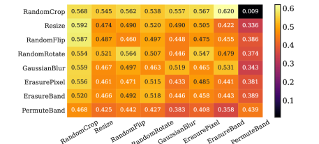
Figure 2: Evaluation under individual or composition of data augmentations on Indian Pines dataset. For all columns, diagonal entries correspond to a single transformation, and off-diagonals correspond to the composition of two transformations.

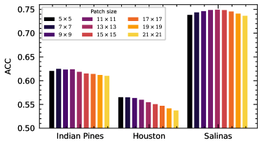
Figure 3: Clustering performance of SSCC with different input patch sizes.

IV-B Comparison with State-of-The-Art Methods

We compare our SSCC model with $12$ representative state-of-the-art clustering approaches, including $k$-means [11], FCM [12], spectral clustering (SC) [54], subspace clustering using least squares regression (LSR) [55], exemplar-based subspace clustering (ESC) [36], hierarchical sparse subspace clustering (HESSC) [56], selective sampling-based scalable sparse subspace clustering (S5C) [35], joint sparse subspace clustering (JSCC) [16], graph convolutional sparse subspace coclustering (GCSSC) [33], AE [57]+$k$-means, DEC [27], and CC [30]. Notably, we include six popular subspace clustering models, four of which (i.e., ESC, HESSC, S5C, and JSCC) are scalable for large datasets. Furthermore, AE+$k$-means, DEC, and CC belong to deep clustering models. Except for JSCC [16] and GCSSC [33], all the compared methods are reproduced under the same preprocessing and follow the settings suggested in the corresponding official releases. Since there are no available codes for JSCC and GCSSC, we compare their results reported in [16] and [33], respectively.

In Table II, III, and IV, we report the comparison results on Indian Pines, Houston, and Salinas datasets, respectively. We can obtain the following three conclusions. First, our SSCC model consistently outperforms other compared methods by large margins across all datasets. For example, ACCs obtained by SSCC on three datasets are $63.05\%$, $56.58\%$, and $78.38\%$ respectively, which improves upon the second-best model (CC on the Indian Pines and Houston, and GCSSC on the Salinas) by a margin of $7.91\%$, $3.10\%$, and $1.72\%$ (absolute differences). For the single cluster’s accuracy (a.k.a., users’ accuracy), SSCC perfectly identifies $3/16$, $2/15$, and $4/16$ land cover types separately on the three datasets. These signify the effectiveness and superiority of our model.

Second, deep clustering models (e.g., AE+$k$-means, DEC, CC, and SSCC) remarkably outperform shallow clustering models (e.g., $k$-means, FCM, and SC). A conceivable reason is that shallow models measure interrelation between raw data directly, thus failing to capture high-level semantic and leading to poor robustness and accuracy. Nonetheless, these classic clustering models can be significantly improved by combining them with deep feature learning. For example, compared to the classic $k$-means, the naive version of AE+$k$-means and its end-to-end version (i.e., DEC) achieve a considerable improvement in terms of clustering accuracy.

Third, SSCC shows better robustness than CC and better scalability than offline clustering models. Compared to CC, the proposed SSCC contains only one prediction head and its architecture is entirely symmetric. Nonetheless, SSCC improves over CC with impressive margins in terms of clustering accuracy across three datasets. This shows that a single projection head and symmetric architecture can also achieve better results by optimizing the proposed loss functions. Compared to offline models (e.g., subspace clustering models), SSCC has an obvious advantage, i.e., ’train once, run everywhere.’ It means SSCC would not be restricted by data sizes and training data. Besides, we can see that out-of-memory (OOM) occurs in SC and LSR in Table IV. This is because both of these methods require computation of a $N\times N$ affinity matrix, which results in quadratic time and space complexity.

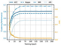
(a)

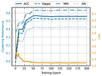
(b)

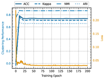
(c)

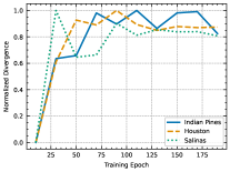
(d)

Figure 4: (a)-(c) Clustering performance of SSCC with increasing epochs on Indian Pines, Houston and Salinas datasets, respectively, where the x-axis denotes the training epoch, the left and right y-axis denote the clustering performance and the corresponding loss value. (d) Quantitative evaluation on the model discriminant power with respect to different epochs by computing the divergence of label representation.

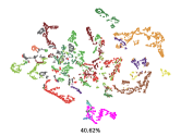
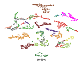
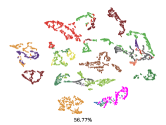
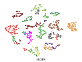
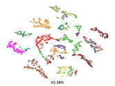
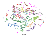
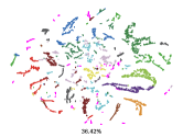
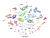
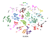
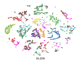
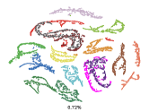
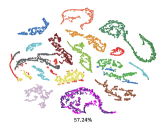
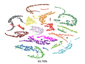
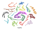
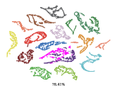
Figure 5: t-SNE visualization on the Indian Pines (the first row), Houston (the second row), and Salinas (third row) datasets with an increasing training iteration. From left to right, the feature representations are obtained at epoch 0, 20, 40, 60, and 100, orderly. Each color indicates a cluster and the clustering ACC value is displayed under each visualization.

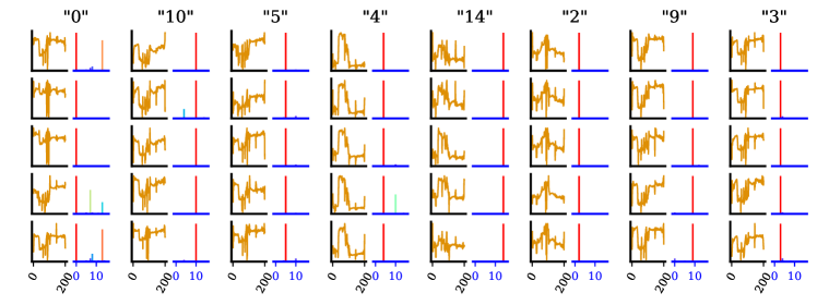
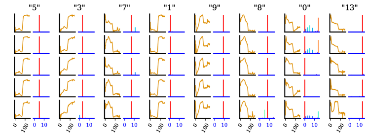
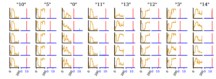
Figure 6: The label representations of the first eight clusters on Indian Pines, Houston, and Salinas datasets. For each dataset, ground-truth labels are written on the upward side, the central spectrum curve of input patches are shown on the left side and corresponding predicted confidences are shown as histograms on the right side. We randomly select $5$ cases from each class.

IV-C Ablation Study and Parameter Analysis

IV-C1 Effect of Components of Objective

To observe the effect of different components in the proposed objective function, we conduct ablation studies on the three datasets by using different combinations of objective terms. Specifically, based on the InfoNCE loss term $\mathcal{L}_{\mathcal{W}}$ and the Barlow Twins loss term $\mathcal{L}_{\mathcal{B}}$, we obtain five loss function combinations: $\mathcal{L}_{\mathcal{W}}$ only, $\mathcal{L}_{\mathcal{B}}$ only, $\mathcal{L}_{\mathcal{W}}+\mathcal{L}_{\mathcal{W}}$, $\mathcal{L}_{\mathcal{B}}+\mathcal{L}_{\mathcal{B}}$ and $\mathcal{L}_{\mathcal{W}}+\mathcal{L}_{\mathcal{B}}$. The first two combinations indicate we only consider either within-cluster loss or between-cluster loss, while the third and the fourth ones signify that both within- and between-cluster loss are implemented using the same formulas as CC [30]. The results are given in Table V. It can be seen that our proposed loss (i.e., $\mathcal{L}_{\mathcal{W}}+\mathcal{L}_{\mathcal{B}}$) achieves more performance gain than others. Nevertheless, single loss terms also show comparable performance by adjusting themselves parameters, demonstrating the discriminative power of contrastive self-supervised learning. Furthermore, the parameters $\tau$ and $\lambda$ involved in $\mathcal{L}_{\mathcal{W}}$ and $\mathcal{L}_{\mathcal{B}}$ showcase different behavior although they have a similar tendency. Following the conclusions in [59] and [40], smaller $\tau$ encourages the model to punish more on hard negative samples, while smaller $\lambda$ tends to maintain the semantic invariability between two views of inputs. The SSCC trained with $\mathcal{L}_{\mathcal{W}}+\mathcal{L}_{\mathcal{W}}$ and $\mathcal{L}_{\mathcal{B}}+\mathcal{L}_{\mathcal{B}}$ cannot achieve significant improvement, even degenerating in the case of $\mathcal{L}_{\mathcal{W}}+\mathcal{L}_{\mathcal{W}}$. It may be because the InfoNCE highly relies on negative samples. In some certain situations, for example, many false-negative samples in a mini-batch, training with $\mathcal{L}_{\mathcal{W}}+\mathcal{L}_{\mathcal{W}}$ would lead to collapsed and unstable representations. That is why $\mathcal{L}_{\mathcal{W}}$ often needs a large batch size for optimizing.

IV-C2 Effect of Batch Size

In order to explore the impact of batch size, we vary it in $\left\{64,128,256,512\right\}$ on three datasets. Table VI shows that larger batch sizes consistently achieve better clustering accuracy and better robustness than smaller ones. Our SSCC model typically belongs to contrastive learning, thus the tendency is consistent with the common observation on such kinds of learning models. As discussed above, a significant reason is that the $\mathcal{L}_{\mathcal{W}}$ objective term requires enough negative pairs in a mini-batch to prevent collapsed representation caused by the false-negative samples. Nevertheless, the usage of Barlow Twins loss alleviates the strong dependency on large batch size by redundancy reduction. We incorporate these two losses together so that they can balance each other in the representation space.

IV-C3 Importance of Data Augmentation

To explore the importance of augmentations, we perform SSCC on the Indian Pines dataset under varying augmentation compositions of RandomCrop, Resize, RandomFlip, RandomRotate, GaussianBlur, ErasurePixel, ErasureBand, and PermuteBand. To better exhibit the influence, we apply only one augmentation operation to each network branch. From Fig. 3, we observe that a single augmentation operation (diagonal entries) is insufficient to guarantee robust clustering accuracy. In contrast, the composition of two augmentation operations shows greater potential in terms of accuracy. In particular, we observe that RandomCrop is more effective than other spatial transformations. Although it increases the difficulty of the contrast task, the spectral transformation has a risk of destroying semantics and leading to the failure of capturing spectral information. As a result, we conduct the spectral transformation with a very small probability. Furthermore, the composition of multiple augmentation operations significantly increases the diversity of data distribution and thus is beneficial to the clustering robustness and accuracy.

IV-C4 Effect of Patch Size

To indicate the effect of input patch sizes, we evaluate the SSCC model by varying input size from $5\times 5$ to $21\times 21$ with an interval of $2\times 2$. Thanks to the architecture of convolutions followed by a global pooling, we can evaluate SSCC using arbitrary patch size without modifying the model. We can observe from Fig. 3 that a suitable patch size is necessary for SSCC to achieve better performance. Generally, HSI patches provide complementary information from views of spectral and spatial, as well as associating the local neighborhood relationship. However, due to the presence of mixed pixels in HSI, there is an increased risk of introducing noisy pixels into input patches when using a large patch size (e.g., $21\times 21$). Furthermore, the problem tends to get worse for HSIs with lower spatial resolution. Consequently, from the results, the patch size should be empirically set to no larger than $13\times 13$.

IV-D Visualization

IV-D1 Convergence Analysis

To analyze the convergence of the SSCC model, Fig. 4 (a)-(c) visualize four clustering metrics against loss values for $200$ training epochs. We observe that clustering metrics are remarkably increased from a relatively low initial value to a stable and superior value, while the loss value tends to be convergent after the $50$-th epoch. This demonstrates that SSCC can gradually capture the spectral-spatial clues by minimizing our defined within- and between-cluster criterion.

To better understand the learning process, we quantify the discriminative power of the learned label representations by defining the following divergence value $S$, i.e.,

$$S=\frac{\sum_{c=1}^{C}\sum_{i\in\mathcal{N}_{c}}s\left(\boldsymbol{y}_{i},\bar{\boldsymbol{y}}_{c}\right)/\left|\mathcal{N}_{c}\right|}{\sum_{c=1}^{C}s\left(\bar{\boldsymbol{y}}_{c},\bar{\boldsymbol{y}}\right)},$$ (7)

where $\bar{\boldsymbol{y}}_{c}$ and $\bar{\boldsymbol{y}}$ indicate the mean vector of the $c$-th class and all samples, respectively, and $\mathcal{N}_{c}$ denotes the index set of the $c$-th class. Following Fisher’s discriminant analysis [60], the numerator and denominator can be treated as within-cluster and between-cluster scatter, respectively. Thus, a larger divergence value means that better separability of the label representation is achieved. In Fig. 4 (d), we show the divergence values by scaling them into $\left[0,1\right]$. As the training epoch increases, the divergence value of label representations is significantly increased, signifying that SSCC’s discriminant ability is enhanced obviously. This also proves why our model can achieve remarkable results for the HSI clustering task.

IV-D2 Latent Representation Visualization

Fig. 5 shows the latent representations (i.e., outputs of the backbone $f_{\theta}\left(\cdot\right)$) for Indian Pines, Houston, and Salinas dataset. In this experiment, we use the t-SNE [61] approach to reduce the dimensionality of latent representations from initially $256$ into $2$. It can be seen that the initial model can roughly separate samples into several limited clusters. Such low-level discriminative ability results in low clustering accuracy. Compared to the initial model, the well-trained model can discover more underlying clusters with a higher clustering accuracy. Furthermore, we can observe that the latent representations at epoch 100 exhibit obvious discriminative capability and uniformity. This superiority is benefited from the mechanism of contrastive learning.

IV-D3 Label Representation Visualization

In Fig. 6, we qualitatively analyze the label representations learned by SSCC on the three HSI datasets. For clarity, we provide both the spectral curve and its corresponding prediction confidence. We observe two obvious tendencies from the visualization. First, the overall prediction confidence of all samples is quite sparse though we didn’t add any sparse regularization. Second, the neuron that indicates the same cluster will be distinctly activated while other neurons will be explicitly inhibited in label representations. These two observations demonstrate that SSCC indeed attempts to capture high-level semantic differences, rather than a simple combination of lower-level representations. In addition, we find that SSCC tends to assign relatively larger confidence to those neurons whose corresponding spectral curves are similar to the true ones, e.g., class 13 and class 14 on the Salinas. This is mainly caused by the spectral variability of HSI. Furthermore, it also may be the main factors that lead to the mis-clustering of those similar land-cover objects.

V Conclusions

We have presented a novel one-stage online SSCC clustering approach for unsupervised learning of large-scale hyperspectral data. The proposed approach follows a contrastive learning pipeline and consists of a spectral-spatial augmentation pool, a backbone network aiming to extract high-level representations and a clustering-specific projection head. We designed a novel objective function based on dual contrastive objectives which implicitly maximizes the within-cluster similarity and minimizes the between-cluster redundancy, simultaneously. The SSCC model is characterized by end-to-end training with mini-batch samples and online clustering, making it scalable to large-scale HSI and possible for being applicable in practice. Experimental results on real HSI datasets show that SSCC can achieve the state-of-the-art clustering performance with remarkable margins over previous works.

The success of SSCC not only narrows the gap between unsupervised methods and supervised methods but also offers a powerful alternative for designing unsupervised methods in the remote sensing community. Future work may include exploring more effective self-supervised schemes to improve the discriminative power and the generalization capability of SSCC to other downstream tasks. For the first problem, an increasing number of self-supervised learning models have been devised recently and some helpful ideas including hard negative mining are worth to be investigated. For the second problem, it is interesting to transfer knowledge from SSCC to other specific tasks, e.g., HSI segmentation and object detection.

References

- [1] P. Ghamisi, N. Yokoya, J. Li, W. Liao, S. Liu, J. Plaza, B. Rasti, and A. Plaza, “Advances in hyperspectral image and signal processing: A comprehensive overview of the state of the art,” IEEE Geoscience and Remote Sensing Magazine, vol. 5, no. 4, pp. 37–78, 2017.
- [2] S. Li, W. Song, L. Fang, Y. Chen, P. Ghamisi, and J. A. Benediktsson, “Deep learning for hyperspectral image classification: An overview,” IEEE Transactions on Geoscience and Remote Sensing, vol. 57, no. 9, pp. 6690–6709, 2019.
- [3] J. Jia, Y. Wang, J. Chen, R. Guo, R. Shu, and J. Wang, “Status and application of advanced airborne hyperspectral imaging technology: A review,” Infrared Physics & Technology, vol. 104, p. 103115, 2020.
- [4] Q. Wang, L. Sun, Y. Wang, M. Zhou, M. Hu, J. Chen, Y. Wen, and Q. Li, “Identification of melanoma from hyperspectral pathology image using 3d convolutional networks,” IEEE Transactions on Medical Imaging, vol. 40, no. 1, pp. 218–227, 2021.
- [5] P. Ghamisi, B. Rasti, N. Yokoya, Q. Wang, B. Hofle, L. Bruzzone, F. Bovolo, M. Chi, K. Anders, R. Gloaguen, P. M. Atkinson, and J. A. Benediktsson, “Multisource and multitemporal data fusion in remote sensing: A comprehensive review of the state of the art,” IEEE Geoscience and Remote Sensing Magazine, vol. 7, no. 1, pp. 6–39, 2019.
- [6] N. Audebert, B. Le Saux, and S. Lefevre, “Deep learning for classification of hyperspectral data: A comparative review,” IEEE Geoscience and Remote Sensing Magazine, vol. 7, no. 2, pp. 159–173, 2019.
- [7] Y. Cai, X. Liu, and Z. Cai, “Bs-nets: An end-to-end framework for band selection of hyperspectral image,” IEEE Transactions on Geoscience and Remote Sensing, vol. 58, no. 3, pp. 1969–1984, 2020.
- [8] S. Jia, S. Jiang, Z. Lin, N. Li, M. Xu, and S. Yu, “A survey: Deep learning for hyperspectral image classification with few labeled samples,” Neurocomputing, vol. 448, pp. 179–204, 2021.
- [9] Y. Cai, Z. Zhang, Z. Cai, X. Liu, X. Jiang, and Q. Yan, “Graph convolutional subspace clustering: A robust subspace clustering framework for hyperspectral image,” IEEE Transactions on Geoscience and Remote Sensing, vol. 59, no. 5, pp. 4191–4202, 2021.
- [10] R. Borsoi, T. Imbiriba, J. C. Bermudez, C. Richard, J. Chanussot, L. Drumetz, J.-Y. Tourneret, A. Zare, and C. Jutten, “Spectral variability in hyperspectral data unmixing: A comprehensive review,” IEEE Geoscience and Remote Sensing Magazine, pp. 2–49, 2021.
- [11] T. Kanungo, D. M. Mount, N. S. Netanyahu, C. D. Piatko, R. Silverman, and A. Y. Wu, “An efficient k-means clustering algorithm: Analysis and implementation,” IEEE transactions on pattern analysis and machine intelligence, vol. 24, no. 7, pp. 881–892, 2002.
- [12] T.-N. Yang, C.-J. Lee, and S.-J. Yen, “Fuzzy objective functions for robust pattern recognition,” in 2009 IEEE International Conference on Fuzzy Systems. IEEE, 2009, pp. 2057–2062.
- [13] E. Elhamifar and R. Vidal, “Sparse subspace clustering: Algorithm, theory, and applications,” IEEE Transactions on Pattern Analysis and Machine Intelligence, vol. 35, no. 11, pp. 2765–2781, 2013.
- [14] R. Vidal and P. Favaro, “Low rank subspace clustering (lrsc),” Pattern Recognition Letters, vol. 43, pp. 47–61, 2014, iCPR2012 Awarded Papers.
- [15] H. Zhang, H. Zhai, L. Zhang, and P. Li, “Spectral-spatial sparse subspace clustering for hyperspectral remote sensing images,” IEEE Transactions on Geoscience and Remote Sensing, vol. 54, no. 6, pp. 3672–3684, 2016.
- [16] H. Zhai, H. Zhang, L. Zhang, and P. Li, “Sparsity-based clustering for large hyperspectral remote sensing images,” IEEE Transactions on Geoscience and Remote Sensing, pp. 1–15, 2020.
- [17] Y. Cai, M. Zeng, Z. Cai, X. Liu, and Z. Zhang, “Graph regularized residual subspace clustering network for hyperspectral image clustering,” Information Sciences, vol. 578, pp. 85–101, 2021.
- [18] J. Lei, X. Li, B. Peng, L. Fang, N. Ling, and Q. Huang, “Deep spatial-spectral subspace clustering for hyperspectral image,” IEEE Transactions on Circuits and Systems for Video Technology, vol. 31, no. 7, pp. 2686–2697, 2021.
- [19] K. Li, Y. Qin, Q. Ling, Y. Wang, Z. Lin, and W. An, “Self-supervised deep subspace clustering for hyperspectral images with adaptive self-expressive coefficient matrix initialization,” IEEE Journal of Selected Topics in Applied Earth Observations and Remote Sensing, vol. 14, pp. 3215–3227, 2021.
- [20] J. Sun, W. Wang, X. Wei, L. Fang, X. Tang, Y. Xu, H. Yu, and W. Yao, “Deep clustering with intraclass distance constraint for hyperspectral images,” IEEE Transactions on Geoscience and Remote Sensing, vol. 59, no. 5, pp. 4135–4149, 2021.
- [21] E. Aljalbout, V. Golkov, Y. Siddiqui, M. Strobel, and D. Cremers, “Clustering with deep learning: Taxonomy and new methods,” arXiv preprint arXiv:1801.07648, 2018.
- [22] E. Min, X. Guo, Q. Liu, G. Zhang, J. Cui, and J. Long, “A survey of clustering with deep learning: From the perspective of network architecture,” IEEE Access, vol. 6, pp. 39 501–39 514, 2018.
- [23] P. Ji, T. Zhang, H. Li, M. Salzmann, and I. Reid, “Deep subspace clustering networks,” in Proceedings of the 31st International Conference on Neural Information Processing Systems, ser. NIPS’17. Red Hook, NY, USA: Curran Associates Inc., 2017, pp. 23–32.
- [24] X. Peng, J. Feng, J. T. Zhou, Y. Lei, and S. Yan, “Deep subspace clustering,” IEEE Transactions on Neural Networks and Learning Systems, vol. 31, no. 12, pp. 5509–5521, 2020.
- [25] J. Lv, Z. Kang, X. Lu, and Z. Xu, “Pseudo-supervised deep subspace clustering,” IEEE Transactions on Image Processing, vol. 30, pp. 5252–5263, 2021.
- [26] M. Jabi, M. Pedersoli, A. Mitiche, and I. B. Ayed, “Deep clustering: On the link between discriminative models and k-means,” IEEE transactions on pattern analysis and machine intelligence, vol. 43, no. 6, pp. 1887–1896, 2019.
- [27] J. Xie, R. Girshick, and A. Farhadi, “Unsupervised deep embedding for clustering analysis,” in Proceedings of The 33rd International Conference on Machine Learning, ser. Proceedings of Machine Learning Research, M. F. Balcan and K. Q. Weinberger, Eds., vol. 48. New York, New York, USA: PMLR, 20–22 Jun 2016, pp. 478–487.
- [28] B. Yang, X. Fu, N. D. Sidiropoulos, and M. Hong, “Towards k-means-friendly spaces: Simultaneous deep learning and clustering,” in Proceedings of the 34th International Conference on Machine Learning, ser. Proceedings of Machine Learning Research, D. Precup and Y. W. Teh, Eds., vol. 70. PMLR, 06–11 Aug 2017, pp. 3861–3870.
- [29] X. Zhan, J. Xie, Z. Liu, Y.-S. Ong, and C. C. Loy, “Online deep clustering for unsupervised representation learning,” in Proceedings of the IEEE/CVF Conference on Computer Vision and Pattern Recognition (CVPR), June 2020.
- [30] Y. Li, P. Hu, Z. Liu, D. Peng, J. T. Zhou, and X. Peng, “Contrastive clustering,” vol. 35, no. 10, May 2021, pp. 8547–8555.
- [31] L. Zhang, L. Zhang, B. Du, J. You, and D. Tao, “Hyperspectral image unsupervised classification by robust manifold matrix factorization,” Information Sciences, vol. 485, pp. 154–169, 2019.
- [32] Y. Qin, B. Li, W. Ni, S. Quan, P. Wang, and H. Bian, “Affinity matrix learning via nonnegative matrix factorization for hyperspectral imagery clustering,” IEEE Journal of Selected Topics in Applied Earth Observations and Remote Sensing, vol. 14, pp. 402–415, 2021.
- [33] N. Huang, L. Xiao, J. Liu, and J. Chanussot, “Graph convolutional sparse subspace coclustering with nonnegative orthogonal factorization for large hyperspectral images,” IEEE Transactions on Geoscience and Remote Sensing, pp. 1–16, 2021.
- [34] R. Wang, F. Nie, Z. Wang, F. He, and X. Li, “Scalable graph-based clustering with nonnegative relaxation for large hyperspectral image,” IEEE Transactions on Geoscience and Remote Sensing, vol. 57, no. 10, pp. 7352–7364, 2019.
- [35] S. Matsushima and M. Brbic, “Selective sampling-based scalable sparse subspace clustering,” in Advances in Neural Information Processing Systems, H. Wallach, H. Larochelle, A. Beygelzimer, F. d'Alché-Buc, E. Fox, and R. Garnett, Eds., vol. 32. Curran Associates, Inc., 2019.
- [36] C. You, C. Li, D. P. Robinson, and R. Vidal, “Scalable exemplar-based subspace clustering on class-imbalanced data,” in Proceedings of the European Conference on Computer Vision (ECCV), September 2018.
- [37] X. Guo, L. Gao, X. Liu, and J. Yin, “Improved deep embedded clustering with local structure preservation,” in Proceedings of the 26th International Joint Conference on Artificial Intelligence, ser. IJCAI’17. AAAI Press, 2017, pp. 1753–1759.
- [38] L. Jing and Y. Tian, “Self-supervised visual feature learning with deep neural networks: A survey,” IEEE Transactions on Pattern Analysis and Machine Intelligence, vol. 43, no. 11, pp. 4037–4058, 2021.
- [39] T. Chen, S. Kornblith, M. Norouzi, and G. Hinton, “A simple framework for contrastive learning of visual representations,” in Proceedings of the 37th International Conference on Machine Learning, ser. Proceedings of Machine Learning Research, H. D. III and A. Singh, Eds., vol. 119. PMLR, 13–18 Jul 2020, pp. 1597–1607.
- [40] J. Zbontar, L. Jing, I. Misra, yann lecun, and S. Deny, “Barlow twins: Self-supervised learning via redundancy reduction,” in ICML 2021: 38th International Conference on Machine Learning, 2021, pp. 12 310–12 320.
- [41] Y. Lin, Y. Gou, Z. Liu, B. Li, J. Lv, and X. Peng, “Completer: Incomplete multi-view clustering via contrastive prediction,” in Proceedings of the IEEE/CVF Conference on Computer Vision and Pattern Recognition (CVPR), June 2021, pp. 11 174–11 183.
- [42] J. Chang, G. Meng, L. Wang, S. Xiang, and C. Pan, “Deep self-evolution clustering,” IEEE Transactions on Pattern Analysis and Machine Intelligence, vol. 42, no. 4, pp. 809–823, 2020.
- [43] A. v. d. Oord, Y. Li, and O. Vinyals, “Representation learning with contrastive predictive coding,” 2018.
- [44] N. Komodakis and S. Gidaris, “Unsupervised representation learning by predicting image rotations,” in International Conference on Learning Representations (ICLR), Vancouver, Canada, Apr. 2018.
- [45] M. Caron, P. Bojanowski, A. Joulin, and M. Douze, “Deep clustering for unsupervised learning of visual features,” in Proceedings of the European Conference on Computer Vision (ECCV), September 2018.
- [46] X. Liu, F. Zhang, Z. Hou, L. Mian, Z. Wang, J. Zhang, and J. Tang, “Self-supervised learning: Generative or contrastive,” IEEE Transactions on Knowledge and Data Engineering, pp. 1–1, 2021.
- [47] J.-B. Grill, F. Strub, F. Altché, C. Tallec, P. H. Richemond, E. Buchatskaya, C. Doersch, B. A. Pires, Z. D. Guo, M. G. Azar, B. Piot, K. Kavukcuoglu, R. Munos, and M. Valko, “Bootstrap Your Own Latent: A new approach to self-supervised learning,” in Neural Information Processing Systems, Montréal, Canada, 2020.
- [48] X. Chen and K. He, “Exploring simple siamese representation learning,” in Proceedings of the IEEE/CVF Conference on Computer Vision and Pattern Recognition (CVPR), June 2021, pp. 15 750–15 758.
- [49] Z. Meng, Z. Yu, K. Xu, and X. Yuan, “Self-supervised neural networks for spectral snapshot compressive imaging,” in Proceedings of the IEEE/CVF International Conference on Computer Vision (ICCV), October 2021, pp. 2622–2631.
- [50] D. Hong, L. Gao, J. Yao, N. Yokoya, J. Chanussot, U. Heiden, and B. Zhang, “Endmember-guided unmixing network (egu-net): A general deep learning framework for self-supervised hyperspectral unmixing,” IEEE Transactions on Neural Networks and Learning Systems, pp. 1–14, 2021.
- [51] J. Yue, L. Fang, H. Rahmani, and P. Ghamisi, “Self-supervised learning with adaptive distillation for hyperspectral image classification,” IEEE Transactions on Geoscience and Remote Sensing, pp. 1–13, 2021.
- [52] H. Zhai, H. Zhang, P. LI, and L. Zhang, “Hyperspectral image clustering: Current achievements and future lines,” IEEE Geoscience and Remote Sensing Magazine, pp. 0–0, 2021.
- [53] K. He, X. Zhang, S. Ren, and J. Sun, “Deep residual learning for image recognition,” in Proceedings of the IEEE Conference on Computer Vision and Pattern Recognition (CVPR), June 2016.
- [54] A. Y. Ng, M. I. Jordan, and Y. Weiss, “On spectral clustering: Analysis and an algorithm,” in Advances in neural information processing systems, 2002, pp. 849–856.
- [55] C.-Y. Lu, H. Min, Z.-Q. Zhao, L. Zhu, D.-S. Huang, and S. Yan, “Robust and efficient subspace segmentation via least squares regression,” in Computer Vision – ECCV 2012, A. Fitzgibbon, S. Lazebnik, P. Perona, Y. Sato, and C. Schmid, Eds. Berlin, Heidelberg: Springer Berlin Heidelberg, 2012, pp. 347–360.
- [56] K. Rafiezadeh Shahi, M. Khodadadzadeh, L. Tusa, P. Ghamisi, R. Tolosana-Delgado, and R. Gloaguen, “Hierarchical sparse subspace clustering (hessc): An automatic approach for hyperspectral image analysis,” Remote Sensing, vol. 12, no. 15, 2020.
- [57] G. E. Hinton and R. R. Salakhutdinov, “Reducing the dimensionality of data with neural networks,” Science, vol. 313, no. 5786, pp. 504–507, 2006.
- [58] H. W. Kuhn, “The hungarian method for the assignment problem,” Naval Research Logistics Quarterly, vol. 2, no. 1-2, pp. 83–97, 1955.
- [59] F. Wang and H. Liu, “Understanding the behaviour of contrastive loss,” in Proceedings of the IEEE/CVF Conference on Computer Vision and Pattern Recognition (CVPR), June 2021, pp. 2495–2504.
- [60] S. Mika, G. Ratsch, J. Weston, B. Scholkopf, and K. Mullers, “Fisher discriminant analysis with kernels,” in Neural Networks for Signal Processing IX: Proceedings of the 1999 IEEE Signal Processing Society Workshop (Cat. No.98TH8468), 1999, pp. 41–48.
- [61] L. Van der Maaten and G. Hinton, “Visualizing data using t-sne.” Journal of machine learning research, vol. 9, no. 11, 2008.