Fully Linear Graph Convolutional Networks for Semi-Supervised Learning and Clustering

Abstract

This paper presents FLGC, a simple yet effective fully linear graph convolutional network for semi-supervised and unsupervised learning. Instead of using gradient descent, we train FLGC based on computing a global optimal closed-form solution with a decoupled procedure, resulting in a generalized linear framework and making it easier to implement, train, and apply. We show that (1) FLGC is powerful to deal with both graph-structured data and regular data, (2) training graph convolutional models with closed-form solutions improve computational efficiency without degrading performance, and (3) FLGC acts as a natural generalization of classic linear models in the non-Euclidean domain, e.g., ridge regression and subspace clustering. Furthermore, we implement a semi-supervised FLGC and an unsupervised FLGC by introducing an initial residual strategy, enabling FLGC to aggregate long-range neighborhoods and alleviate over-smoothing. We compare our semi-supervised and unsupervised FLGCs against many state-of-the-art methods on a variety of classification and clustering benchmarks, demonstrating that the proposed FLGC models consistently outperform previous methods in terms of accuracy, robustness, and learning efficiency. The core code of our FLGC is released at https://github.com/AngryCai/FLGC.

I Introduction

Graph neural network (GNN) has emerged as a powerful technique for the representation learning of graphs [1, 2]. Current GNN models usually follow a neighborhood aggregation scheme, where the feature representation of a node is updated by recursively aggregating representation vectors of its neighbors [3, 4]. Benefited from the promising ability to model graph structural data, traditional learning problems can be revisited from the perspective of graph representation learning, ranging from recommendation [5] and computer vision [6, 7, 8], to combinatorial optimization [9, 10].

In recent years, there is increasing attention for generalizing convolution to the graph domain. The existing graph convolutional networks (GCNs) often broadly categorize into spectral approaches and spatial approaches [2, 4]. Spectral models commonly use the spectral graph theory to design spectral filters, such as ChebyNet [11] and the vanilla GCN [12]. While spatial models define graph convolutions based on a node’s spatial relations, e.g., GraphSAGE [13, 14] and Graph Attention networks (GAT) [15]. Due to the good theoretical guarantee, spectral models have been extensively studied by the recent mainstream. Despite their success, most of the state-of-the-art (SOTA) GCN models are dominated by shallow and simple models because of the over-smoothing problem [3, 16]. To circumvent the problem, many efforts have been paid to develop deeper and more robust models. The proven techniques include residual connection [16], randomly drop nodes [17] or edges [18], and data augmentation [19], etc.

More recent attempts in simplifying GCN have collectively suggested that a GCN model can be decoupled into two successive stages: parameter-free neighborhood propagation and task-specific prediction. Following this scheme, Wu et al. [20] initially proposed Simple Graph Convolution (SGC) [20] by simplifying the vanilla GCN as a low-pass filter followed by a linear classifier. While Approximate Personalized Propagation of Neural Predictions (APPNP) [21] swaps the two stages and establishes a connection between GCN and the well-known PageRank [22]. These successful attempts signify several helpful tendencies. First, simplified GCNs have a similar capability to the elaborated ones in handling structural data. Second, a linear GCN is as powerful as the nonlinear counterpart for most graph scenarios. Nonetheless, fewer studies have managed to develop a unified framework between traditional linear models and GCNs. Moreover, gradient descent-based training of simplified GCNs often suffers from local optimum, tedious hyper-parameters and training tricks. Hence, it would result in a more simplified GCN if a globally optimal solution in a closed form is provided.

Earlier linear models, such as ridge regression [23] and subspace clustering [24], have been frequently applied in practice owing to their simplicity, efficiency, and efficacy. However, these classic models essentially work in the Euclidean domain, leading to insufficient handling of graph structured data. Before GCNs emerged, graph Laplacian regularization (or manifold regularization) [25, 26] had been widely applied in various linear models to incorporate structural information. This inspires a series of classic graph-regularized semi-supervised approaches, e.g., Laplacian Regularized Least Squares (LapRLS) [25], and graph-regularized unsupervised approaches, e.g., Laplacian Regularized Low-Rank Representation [27]. Despite being a useful technique, the Laplacian regularization encounters three shortcomings: 1) it is typically dependent upon the Euclidean domain and, thus, it is hard to directly generalize to real-word graph data; 2) it merely considers the 1^st-order neighborhoods while ignoring important long-range interdependency; 3) its additional regularization coefficient needs to be appropriately adjusted.

In this paper, we propose a very simple and unified framework, referred to as Fully Linear Graph Convolution (FLGC), for both semi-supervised learning (SSL) and unsupervised learning (USL). Our goal is to further simplify GCNs and generalize it to existing linear models, finally enabling traditional models to explore graphs directly. Specifically, we linearize GCN and then decouple it into neighborhood propagation and prediction stages, resulting in a flexible framework. Such simplification makes it possible to efficiently calculate a globally optimal solution during training and also easy to incorporate with various previous linear models. On the basis of the resulting framework, we further present a semi-supervised FLGC for node classification problems and an unsupervised FLGC for subspace clustering problems. To prevent the over-smoothing issue, we introduce an initial residual in neighborhood propagation to capture the long-range dependency across a graph.

To sum up, the main contributions of this paper are as follows:

1. We present a simple yet effective FLGC framework to deal with graph data and regular data. The framework consists of a parameter-free neighborhood propagation and a task-specific linear model with a closed-form solution. The framework not only simplifies the training of existing GCNs with a general but makes it easier to implement and apply in practice.

2. We implement two FLGCs for semi-supervised node classification and unsupervised clustering tasks, respectively. Also, we show that the semi-supervised and unsupervised FLGCs act as a generalization of classic ridge regression and subspace clustering in the non-Euclidean domain. Such generalization enables traditional linear models to explore graph structure without losing their original simplicity and efficacy.

3. We extend the personalized propagation scheme to balance the contribution of structure and node features, which endows FLGC with the capability of capturing long-range neighborhoods, thereby reducing the risk of over-smoothing.

4. We empirically show that FLGCs consistently outperform a large number of previous SOTA approaches on both semi-supervised learning and clustering tasks across real-world graph data and regular grid data. Such superiority further offers a promising scheme to revisit traditional linear models in a pure non-Euclidean domain.

The rest of the paper is structured as follows. In Section II, we briefly review the related concepts on recent GCN models and subspace clustering. Section III systematically introduces the motivation, framework, formulation, and implementation of the proposed FLGCs. Extensive qualitative and quantitative evaluations and comparisons are presented in Section IV and Section V, followed by the conclusions. Conclusions and future works are given in Section VI.

II Notation and Concepts

II-A Notations

In this paper, boldface lowercase italics symbols (e.g., $\boldsymbol{x}$), boldface uppercase roman symbols (e.g., $\mathbf{X}$), regular italics symbols (e.g., $N$), and calligraphy symbols (e.g., $\mathcal{S}$) orderly denote vectors, matrices, scalars, and sets. A graph is represented as $\mathcal{G}=(\mathcal{V},\mathcal{E},\mathbf{X})$, where $\mathcal{V}$ denotes the node set with $v_{i}\in\mathcal{V}$ and $\left|\mathcal{V}\right|=N$, $\mathcal{E}$ indicates the edge set with $\left(v_{i},v_{i}\right)\in\mathcal{E}$, and $\mathbf{X}\in\mathbb{R}^{N\times D}$ signifies the $D$-dimensional node feature matrix of $\mathcal{G}$ while the corresponding $C$-class one-hot target matrix is $\mathbf{Y}\in\mathbb{R}^{N\times C}$. We define $\mathbf{A}\in\mathbb{R}^{N\times N}$ as the adjacency matrix of $\mathcal{G}$ and the diagonal degree matrix as $\mathbf{D}\in\mathbb{R}^{N\times N}$, where $D_{ii}=\sum_{j}A_{ij}$. The graph Laplacian matrix is defined as $\mathbf{L}=\mathbf{D}-\mathbf{A}$, and its normalized version is given by $\mathbf{L}_{sym}=\mathbf{D}^{-1/2}\mathbf{L}\mathbf{D}^{-1/2}$, which has an eigendecomposition of $\mathbf{U}\boldsymbol{\Lambda}\mathbf{U}^{T}$. Here, $\boldsymbol{\Lambda}$ is a diagonal matrix of the eigenvalues of $\mathbf{L}$, and $\mathbf{U}$ is a unitary matrix consisting of the eigenvectors of $\mathbf{L}$. Bedsides, $\mathbf{X}^{T}$ denotes the transpose of matrix $\mathbf{X}$ and $\mathbf{I}_{N}$ denotes an identity matrix with the size of $N$. The trace operation and the Frobenius norm of matrix $\mathbf{X}$ are defined as $\mathrm{tr}\left(\mathbf{X}\right)$ and $\mathbf{\left\|X\right\|}_{F}=\sqrt{\mathrm{tr}\left(\mathbf{X}^{T}\mathbf{X}\right)}$, respectively.

II-B Vanilla GCN

We refer to the GCN model proposed by Kipf et al. [12] as the vanilla GCN because of its great success and numerous followers. The vanilla GCN suggests that the graph convolution operation can be approximated by the $K$-th order polynomial of Laplacians, i.e.,

$$\mathbf{U}g_{\theta}\mathbf{U}^{T}\boldsymbol{x}\approx\mathbf{U}\left(\stackrel{{\scriptstyle[}}{{i}}=0]{K}{\sum}\theta_{i}\boldsymbol{\Lambda}^{\left(i\right)}\right)\mathbf{U}^{T}\boldsymbol{x}=\left(\stackrel{{\scriptstyle[}}{{i}}=0]{K}{\sum}\theta_{i}\mathbf{L}^{\left(i\right)}\right)\boldsymbol{x},$$ (1)

where $g_{\theta}=diag\left(\theta\right)$ is a graph filter parameterized by $\theta\in\mathbb{R}^{N}$ in the Fourier domain and $\theta_{i}$ denotes the polynomial coefficient. The vanilla GCN [12] adopts two crucial strategies to simplify and enhance Eq. (1). First, it uses a 1^st-order polynomial with settings of $\theta_{0}=2\theta$ and $\theta_{1}=-\theta$ to approximate Eq. (1), resulting in a simplified convolution operation, i.e., $g_{\theta}*\boldsymbol{x}=\theta\left(\mathbf{I}+\mathbf{D}^{-1/2}\mathbf{A}\mathbf{D}^{-1/2}\right)\boldsymbol{x}$. Second, it introduces a renormalization trick to guarantee its stability. Specifically, the trick can be expressed as

$$\mathbf{P}=\left(\mathbf{D}+\mathbf{I}\right)^{-1/2}\left(\mathbf{A}+\mathbf{I}\right)\mathbf{\left(\mathbf{D}+\mathbf{I}\right)}^{-1/2}=\tilde{\mathbf{D}}^{-1/2}\mathbf{\tilde{A}}\mathbf{\tilde{D}}^{-1/2}.$$ (2)

We call $\mathbf{P}$ as propagation matrix. As a result, in analogy to convolutional neural networks (CNN) [28, 29], a general and layer-wise graph convolution propagation rule can be defined by

$$\mathbf{\mathbf{X}^{\left(\ell+1\right)}}=\mathrm{ReLU}\left(\mathbf{P}\mathbf{X}^{\left(\ell\right)}\mathbf{W}^{\left(\ell\right)}\right).$$ (3)

Here, $\mathbf{X}^{\left(\ell\right)}$ is the $\ell$-th layer’s graph embedding ($\mathbf{X}^{\left(1\right)}=\mathbf{X}$) and $\mathbf{W}^{\left(\ell\right)}$ is a trainable parameters matrix. However, many works [2, 3, 20, 21, 4, 16] have demonstrated that stacking multiple GCN layers will lead to the over-smoothing effect, that is to say, all vertices will converge to the same value. Thus, the vanilla GCN usually adopts a shallow architecture, e.g., two GCN layers.

II-C SGC

SGC [20] removes nonlinear activations in the vanilla GCN and collapses all trainable weights into a single matrix. This enables it to raise the repeated multiplication of the normalized adjacency matrix $\mathbf{P}$ as a $K$-th power of a matrix, i.e.,

$$\begin{aligned} \tilde{\mathbf{Y}}&=\mathrm{softmax}\left(\underset{K}{\underbrace{\mathbf{P}\mathbf{P}\cdots\mathbf{P}}}\mathbf{\mathbf{X}}\underset{K}{\underbrace{\mathbf{W}_{1}\mathbf{W}_{2}\cdots\mathbf{W}_{K}}}\right)\\ &=\mathrm{softmax}\left(\mathbf{P}^{K}\mathbf{\mathbf{X}}\mathbf{W}\right)\end{aligned}.$$ (4)

Furthermore, SGC can be regarded as a fixed feature extraction/smoothing component $\tilde{\mathbf{X}}=\mathbf{P}^{K}\mathbf{\mathbf{X}}$ followed by a linear logistic regression classifier $\tilde{\mathbf{Y}}=\mathrm{softmax}\left(\tilde{\mathbf{\mathbf{X}}}\mathbf{W}\right)$. In [20], Wu et al. suggested that SGC acts as a low-pass filter and such a signified model performs comparably to many SOTA models.

II-D APPNP

Personalized propagation of neural predictions (PPNP) and its fast approximation, APPNP [21], consider the relationship between GCN and PageRank to derive an improved propagation scheme based on personalized PageRank. Let $\mathbf{H}^{(0)}=h_{\theta}\left(\mathbf{X}\right)$ be a multilayer perceptron (MLP) parameterized by $\theta$. Then PPNP is defined as

$$\tilde{\mathbf{Y}}=\mathrm{softmax}\left(\alpha\left(\mathbf{I}-(1-\alpha)\mathbf{P}\right)^{-1}\mathbf{H}^{(0)}\right),$$ (5)

where $\alpha\in(0,1]$ is the teleport (or restart) probability of the topic-sensitive PageRank.

Similar to SGC, PPNP separates the neural network used for generating predictions from the propagation scheme. While APPNP further approximates topic-sensitive PageRank via power iteration, i.e.,

$$\begin{array}[]{c}\mathbf{H}^{(i)}=\alpha\mathbf{H}^{(0)}+\left(1-\alpha\right)\mathbf{P}\mathbf{H}^{(i-1)}\\ \tilde{\mathbf{Y}}=\mathrm{softmax}\left(\alpha\mathbf{H}^{(0)}+\left(1-\alpha\right)\mathbf{P}\mathbf{H}^{(K-1)}\right)\end{array}.$$ (6)

One of the great advantages of PPNP and APPNP is that they decouple feature transformation and propagation procedures of the vanilla GCN without increasing the number of trainable parameters.

II-E Classic Linear Models

We broadly divide classic linear models into supervised methods and unsupervised methods. Similar to SGC, a typical supervised linear model can be treated as a fully linearized MLP, given by

$$\mathbf{\mathbf{X}}_{\mathcal{T}}\mathbf{W}_{1}\mathbf{W}_{2}\cdots\mathbf{W}_{\ell}=\mathbf{\mathbf{X}}_{\mathcal{T}}\mathbf{W}=\mathbf{Y}_{\mathcal{T}}.$$ (7)

Here, $\mathbf{\mathbf{X}}_{\mathcal{T}}$ and $\mathbf{Y}_{\mathcal{T}}$ denote training samples and corresponding target matrix, respectively. Such a model is also known as a ridge regression classifier [23, 30]. Besides, logistic regression and softmax regression are its two most frequently-used variants in deep neural networks [31, 1, 32, 28, 33].

The unsupervised fashion of a linear model often follows a common assumption, i.e., data points lie in a union of linear subspaces. While the subspace representation coefficients $\mathbf{Z}\in\mathbb{R}^{N\times N}$ can be obtained by solving the following linear self-expressive model, i.e.,

$$\mathbf{\mathbf{X}}^{T}\mathbf{Z}=\mathbf{X}^{T},~{}s.t.~{}diag\left(\mathbf{Z}\right)=0$$ (8)

Notably, the main difference between Eq. (7) and Eq. (8) is that the former considers the combination between every feature, while the latter considers samples. In order to achieve an effective solution, various norm constraints are often imposed on $\mathbf{W}$ or $\mathbf{Z}$. Sparse Subspace Clustering (SSC) [24] utilizes an $\ell_{1}$ norm $\left\|\mathbf{Z}\right\|_{1}$, while Low Rank Subspace Clustering (LRSC) [34] adopts a nuclear norm $\left\|\mathbf{Z}\right\|_{*}$, just to name a few. Despite their success, the objective functions derived from these constraints are not smooth, leading to inefficient solutions. In contrast, the Frobenius norm $\left\|\mathbf{Z}\right\|_{F}$ will result in a closed-form solution for linear models.

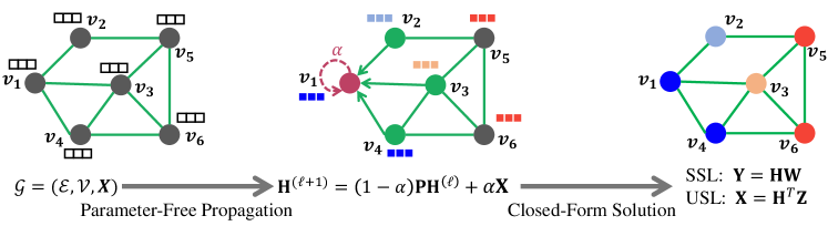
(a) Graph-form Illustration of our FLGC framework. FLGC first performs parameter-free propagation which aggregates multi-hop neighboring information with a power iteration of propagation matrix $\mathbf{P}$ and then predicts node labels by calculating a closed-form solution (affinity matrix).

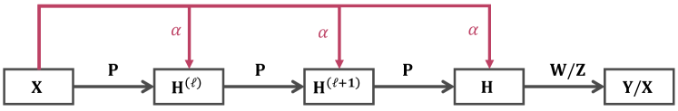
(b) Matrix-form data flow of FLGC. It can be seen that FLGC conducts a personalized multi-hop propagation operation with a fixed propagation matrix $\mathbf{P}$, followed by a linear model parameterized by a weight matrix $\mathbf{W}$ for semi-supervised classification or a coefficient matrix $\mathbf{Z}$ for unsupervised classification.

Figure 1: Schematic representations of our proposed FLGC.

III Fully Linear Graph Convolutional Networks

We present the general FLGC framework for semi-supervised classification and unsupervised classification problems, as illustrated in Fig. 1 (a). The core behind our FLGC is to generalize GCNs to traditional linear models so that a) training linear GCN model with global optimal solution b) enabling traditional linear models to work on graph-structured data, 3) further simplifying the existing GCN models.

III-A Fully Linearization of GCN

Inspired by the SGC [20] model, we further remove all nonlinear operations of a $K$-layer GCN, including the logistic regression classifier. It derives the following linear GCN

$$\mathbf{P}^{K}\mathbf{\mathbf{X}}\mathbf{W}=\mathbf{\tilde{Y}}.$$ (9)

This linearization brings three major benefits. First, it is easy to decouple the fully linear GCN into two stages: a parameter-free feature propagation stage (i.e., $\mathbf{H}=\mathbf{P}^{K}\mathbf{\mathbf{X}}$, where $\mathbf{H}$ denotes graph embedding) and a target-dependent prediction stage (i.e., $\mathbf{\tilde{Y}}=\mathbf{H}\mathbf{W}$). The former aggregates $K$-hop neighborhoods based on a predefined propagation matrix $\mathbf{P}$. While the later acts as a ridge regression classifier parameterized by $\mathbf{W}$. Second, it establishes a relationship between traditional linear models and GCN models. This relationship enables us to reconsider the traditional linear models from the graph representation learning point of view. Also, it endows the classic ridge regression classifier with the ability to handle graphs directly. Third, the linearization makes it possible to efficiently solve the global optimal solution of GCN without using gradient descent. We refer to such GCN as Fully Linear Graph Convolution (FLGC). A matrix-form data flow of FLGC is depicted in Fig. 1 (b). More details will be introduced as follows.

III-B Multi-hop Propagation

In light of the aforementioned linearization, we can define various propagation strategies and incorporate them into Eq. (9). Here we introduce a stable propagation scheme for our FLGC. According to the spectral graph theory, $\underset{K\rightarrow\infty}{\lim}\mathbf{P}^{K}\mathbf{X}$ will converge to a stationary state as the number of propagation steps increases [21, 16]. While the node representations on the same connected component of a graph become indistinguishable, i.e., over-smoothing problem [21, 16]. Moreover, $\mathbf{P}^{K}\mathbf{X}$ serves as a structure aggregation term and ignores the importance of initial node features. The initial node features often imply unique discriminant information, especially for those data without directly available graph structures.

To balance the structure between initial features, we adopt an extended APPNP’s propagation scheme to propagate multi-hop neighboring information. The propagation procedure with $K$ power iteration is recursively calculated by

$$\begin{array}[]{c}\mathbf{H}^{\left(\ell+1\right)}=\left(1-\alpha\right)\mathbf{P}\mathbf{H}^{\left(\ell\right)}+\alpha\mathbf{X}\\ s.t.~{}\mathbf{H}^{\left(1\right)}=\mathbf{X},~{}\ell=1,\cdots,K\end{array}.$$ (10)

Instead of using a neural network to generate a prediction as it is done in APPNP [21], we directly use the initial $\mathbf{X}$ as topics to be ranked in the topic-sensitive PageRank [22]. Let the resulting final graph embedding be $\mathbf{H}=\mathbf{H}^{\left(K\right)}$. This ensures that $\mathbf{H}$ is always contributed by both structure and initial features with a fixed proportion $\alpha$. It is trivial to prove that SGC’s propagation (i.e., Eq. (9)) is a special case of Eq. (10) with $\alpha=0$. Furthermore, when $\alpha=1$, SGC degrades into an ordinary neural network, in which no structural information is used. From the residual network’s point of view [12, 16, 35], our propagation scheme is a special form of residual connection, where each forward step connects with initial inputs and weighted by $\alpha$ [as shown in Fig. 1 (b)]. Thus, our propagation mechanism is also called initial residual [16].

III-C FLGC for Semi-Supervised Learning

Having introduced the FLFC framework, we are ready to calculate the closed-form solution for a specific downstream task. We first use the FLGC for the semi-supervised node classification problem. Let $\hat{\mathbf{Y}}\in\mathbb{R}^{N\times C}$ be an augmented target matrix, where labeled nodes are presented as one-hot vectors while unlabeled nodes are marked as zero vectors. Further let $\mathbf{M}$ be a diagonal mask matrix associated with the labeled and unlabeled nodes. Thus, the semi-supervised FLGC can be denoted by

$$\mathbf{H}\mathbf{W}=\mathbf{\hat{\mathbf{Y}}}.$$ (11)

To effectively solve this problem, we rewrite the objective function as a Frobenius norm minimization problem, i.e.,

$$\underset{\mathbf{W}}{\arg\min}\left\|\mathbf{W}\right\|_{F},~{}s.t.~{}\mathbf{H}\mathbf{W}=\widetilde{\mathbf{Y}}.$$ (12)

The problem can be further expressed in the following form by using the Lagrangian multiplier

$$\begin{aligned} \underset{\mathbf{W}}{\arg\min~{}}\mathcal{L}=&\frac{1}{2}\left\|\mathbf{M}^{1/2}\left(\mathbf{H}\mathbf{W}-\mathbf{\hat{\mathbf{Y}}}\right)\right\|_{F}^{2}+\frac{\lambda}{2}\left\|\mathbf{W}\right\|_{F}^{2}\\ =&\frac{1}{2}\mathrm{tr}(\mathbf{W}^{T}\mathbf{H}{}^{T}\mathbf{M}\mathbf{H}\mathbf{W}+\mathbf{\hat{\mathbf{Y}}}^{T}\mathbf{M}\mathbf{\hat{\mathbf{Y}}}-\\ &2\mathbf{\hat{\mathbf{Y}}}^{T}\mathbf{M}\mathbf{H}\mathbf{W}+\lambda\mathbf{W}^{T}\mathbf{W})\end{aligned},$$ (13)

where $\lambda$ denotes a regularization coefficient. The partial derivative of $\mathcal{L}$ with respect to $\mathbf{W}$ is

$$\begin{aligned} \frac{\partial\mathcal{L}}{\partial\mathbf{W}}=&\left(\mathbf{H}^{T}\mathbf{M}\mathbf{H}\mathbf{W}-\mathbf{H}^{T}\mathbf{M}\mathbf{\hat{\mathbf{Y}}}+\lambda\mathbf{W}\right)\end{aligned}.$$ (14)

The global optimal solution is derived when $\frac{\partial\mathcal{L}}{\partial\mathbf{W}}=0$, i.e.,

$$\mathbf{H}^{T}\mathbf{M}\mathbf{H}\mathbf{W}-\mathbf{H}^{T}\mathbf{M}\mathbf{\hat{\mathbf{Y}}}+\lambda\mathbf{W} =0$$ (15)

Consequently, we denote the solution in closed form as

$$\boldsymbol{\mathbf{W}}^{*}=\left(\mathbf{H}^{T}\mathbf{M}\mathbf{H}+\lambda\mathbf{I}_{D}\right)^{-1}\mathbf{H}^{T}\mathbf{M}\mathbf{\hat{\mathbf{Y}}}.$$ (16)

Finally, we infer the test node’s labels via a transductive manner.

III-D FLGC for Clustering

Our unsupervised FLGC follows the classic subspace clustering by assuming that the $K$-hop graph embeddings lie in a union of $C$ subspaces. More precisely, every node belonging to a certain subspace can be explicitly represented using other nodes in this subspace while subspaces do not interact with each other. We refer to this property of data as self-expressiveness. However, using an initial input to model such a property may lead to an unreliable estimate of subspace coefficients due to outliers and noisy points. Instead, we model our unsupervised FLGC based on the graph embedding of inputs. The motivation behind our method is that the intra-class variation of the initial inputs can be smoothed by using the graph convolution. Formally, we express our unsupervised FLGC as follows

$$\underset{\mathbf{Z}}{\arg\min~{}}\left\|\mathbf{Z}\right\|_{q},~{}s.t.~{}\mathbf{H}^{T}\mathbf{Z}=\mathbf{X}^{T},\mathrm{diag}\left(\mathbf{Z}\right)=0$$ (17)

Here, $\mathbf{Z}\in\mathbb{R}^{N\times N}$ is an affinity matrix, in which the $j$-th column denotes the representation coefficient vector of node $v_{j}$, and $q$ indicates the $q$-norm of a matrix. By analogy with classic subspace clustering models, $q=1$ will lead to a standard sparse subspace representation while replacing $q$ with the nuclear norm will derive a low-rank subspace representation.

In this paper, we aim to calculate a dense subspace representation by adopting the Frobenius norm, as well as maintaining the consistency of our FLGC framework. It has been proven [36] that the constraint $\mathrm{diag}\left(\mathbf{Z}\right)=0$ can be relaxed and discarded by using a Frobenius norm. Hence, our unsupervised FLGC can be rewritten as

$$\begin{aligned} \underset{\mathbf{Z}}{\arg\min~{}}\mathcal{L}=\frac{1}{2}\left\|\mathbf{H}^{T}\mathbf{Z}-\mathbf{X}^{T}\right\|_{F}^{2}+\frac{\lambda}{2}\left\|\mathbf{Z}\right\|_{F}^{2}=\\ \mathrm{tr}\left(\mathbf{Z}^{T}\mathbf{H}\mathbf{H}^{T}+\mathbf{X}^{T}\mathbf{X}-2\mathbf{X}\mathbf{H}^{T}\mathbf{Z}+\frac{\lambda}{2}\mathbf{Z}^{T}\mathbf{Z}\right)\end{aligned}.$$ (18)

We further compute $\frac{\partial\mathcal{L}}{\partial\mathbf{W}}$ as

$$\frac{\partial\mathcal{L}}{\partial\mathbf{Z}}=\left(\mathbf{H}\mathbf{H}^{T}\mathbf{Z}-\mathbf{H}\mathbf{X}^{T}+\lambda\mathbf{Z}\right).$$ (19)

Similar to the semi-supervised FLGC, we can give the global optimal closed-form solution of Eq. (18), i.e.,

$$\boldsymbol{\mathbf{Z}}^{*}=\left(\mathbf{H}\mathbf{H}^{T}+\lambda\mathbf{I}_{N}\right)^{-1}\mathbf{H}\mathbf{X}^{T}.$$ (20)

Following [7] and [7], we perform the spectral clustering on $\boldsymbol{\mathbf{Z}}^{*}$ to segment subspaces after using a block-structure heuristic.

III-E Remarks on FLGC

In Algorithm refalg:pesudocode, we provide the pseudocode for our semi-supervised and unsupervised FLGC. Noticed that both methods share a unified learning procedure and are easy to implement and train. In reality, our proposed FLGC models can be treated as natural generalizations of classic linear models in the non-Euclidean domain.

Algorithm 1 Pseudocode of FLGC in a PyTorch-like style.
# lambda: regularization coefficient
# alpha: teleport (or restart) probability
#
# fit: calculate closed form solutions
# sc: spectral clustering
# mm: matrix-matrix multiplication
# gcn_norm: normlize adjacency matrix
# compute augmented normalized adjacency
P = gcn_norm(A) # NxD
# compute K-hop graph embedding
H = X # NxD
for i range(K):
# propagate neighborhood using Eq.(10)
H = (1 - alpha) * mm(A_hat, H) + alpha * X # NxD
# SEMI-SUPERVISED FLGC
if task == ’ssl’:
# compute W using Eq.(16)
W = fit(H, Y_aug, M) # DxC
# predict unlabeled nodes
y = mm(H, W)
# UNSUPERVISED FLGC
elif task == ’usl’:
# compute Z using Eq.(20)
Z = fit(H, X)
# assign node labels through spectral clustering
y = sc(Z)

Let $\mathcal{F_{\varTheta}}\left(\mathcal{G}\right)$ be the generalized linear learning model defined on a graph $\mathcal{G}$. FLGC can be broadly denoted as a classic model, $f_{\varTheta}$, multiplied by a $K$-hop propagation matrix, $\mathcal{P}_{K}$, i.e.,

$$\mathcal{F_{\varTheta}}\left(\mathcal{G}\right)=\mathcal{P}_{K}\left(\mathbf{A}\right)f_{\varTheta}\left(\mathbf{X}\right).$$ (21)

The only trainable parameter, $\varTheta$, is derived from the classic model which can be solved in a similar manner to the existing models. It is easy to prove that FLGC is a generalization of classic linear models in the non-Euclidean domain. When $\mathcal{P}_{K}\left(\mathbf{A}\right)=\mathbf{I}$, signifying that $\mathcal{G}$ does not have any edges except for self-loops, FLGC is equivalent to classic linear models. Benefited from the decoupled design, $\mathcal{P}_{K}\left(\mathbf{A}\right)$ is target-independent and can be precomputed. Thus, FLGC does not increase the computational burden compared to the classic linear models. Here, we show the connections of FLGC to existing models.

• FLGC v.s. Manifold Regularization Let $\mathcal{L}_{MR}=\mathcal{O}_{emp}\left(f\right)+\lambda\mathcal{R}_{srm}\left(\varTheta\right)+\gamma\mathcal{R}_{pri}\left(f\right)$ be the objective function of a manifold regularized model, where $\mathcal{O}_{emp}$, $\mathcal{R}_{srm}$, and $\mathcal{R}_{pri}$ denote the empirical error term, the structural risk term, and the manifold prior term, orderly. Further let $\mathcal{L}_{FLGC}=\mathcal{O}_{emp}\left(\mathcal{F}\right)+\lambda\mathcal{R}_{srm}\left(\varTheta\right)$ be the proposed FLGC. As suggested in [37], both $\mathcal{L}_{MR}$ and $\mathcal{L}_{FLGC}$ are derived from the same optimization framework. Nonetheless, there is a considerable difference between them. That is, our FLGC directly works in the non-Euclidean domain, while the manifold regularization is proposed for Euclidean data. During the learning, manifold regularized models use the graph structure as the prior knowledge, generally defined as $\mathcal{R}_{pri}=\mathrm{tr}\left(f^{T}\mathbf{L}f\right)$, which is incorporated as a single term balanced by an additional regularization coefficient. In particular, the manifold regularization cannot model the long-range relationships. In contrast, our FLGC propagates multi-hop structural information in a more general and flexible manner.

• FLGC v.s. AutoEncoder Our unsupervised FLGC is highly related to linear autoencoders [7]. We define a linear graph autoencoder as $\mathcal{D}_{\mathbf{Z}}\left(\mathcal{E}_{\varTheta}\left(\mathcal{G}\right)\right)=\mathbf{X}$, where $\mathcal{E}_{\varTheta}$ and $\mathcal{D}_{\mathbf{Z}}$ are the decoder and encoder, respectively. By collapsing weights matrices of a $K$-layer encoder in a single matrix $\varTheta$, an autoencoder with a self-expressive layer becomes $\mathcal{E}_{\varTheta}=\varTheta\mathbf{X}^{T}\mathbf{P}^{K}=\mathbf{H}$ and $\mathcal{D}_{\mathbf{Z}}=\mathbf{H}\mathbf{Z}=\mathbf{X}$. By replacing $\varTheta$ using a fixed unitary matrix $\mathbf{I}$, such encoder becomes the propagation stage of the unsupervised FLGC, while our $\mathcal{D}_{\mathbf{Z}}$ is a single layer self-expression. Furthermore, our FLGC aims to reconstruct node features rather than the structure that adopted in the graph autoencoder [38].

IV Experiments of SSL

In this section, we compare the proposed semi-supervised FLGC model against many SOTAs and classic methods on 3 real-world graph benchmark datasets and 24 regular UCI datasets. Furthermore, numerous ablation experiments are conducted to systematically and comprehensively analyze the effectiveness and robustness of the proposed FLGC.

TABLE I: Summary of citation network datasets.

Dataset	#Nodes	#Edges	#Classes	#Features	Train/Dev/Test
Cora	2,708	5,429	7	1433	140/500/1,000
Citeseer	3,327	4,732	6	3703	120/500/1,000
Pubmed	19,717	44,338	3	500	60/500/1,000

TABLE II: Summary of baseline comparison under public splits for Cora, Citeseer, and Pubmed. FLGC* corresponds to FLGC with $\alpha=0.1$. The results at the top are collected from literature while the middle is reproduced according to our settings.

Method	Cora	Citeseer	PubMed
GCN	81.4 $\pm$0.4	70.9 $\pm$0.5	79.0 $\pm$0.4
GAT	83.3 $\pm$0.7	72.6 $\pm$0.6	78.5 $\pm$0.3
FastGCN	79.8 $\pm$0.3	68.8 $\pm$0.6	77.4 $\pm$0.3
GIN	77.6 $\pm$1.1	66.1 $\pm$0.9	77.0 $\pm$1.2
LNet	80.2 $\pm$3.0	67.3 $\pm$0.5	78.3 $\pm$0.6
AdaLNet	81.9 $\pm$1.9	70.6 $\pm$0.8	77.8 $\pm$0.7
DGI	82.5 $\pm$0.7	71.6 $\pm$0.7	78.4 $\pm$0.7
SGC	81.0$\pm$0.0	71.9 $\pm$0.1	78.9 $\pm$0.0
MixHop	81.9$\pm$ 0.4	71.4$\pm$0.8	80.8$\pm$0.6
DropEdge	82.8	72.3	79.6
G3NN	82.5$\pm$0.2	74.4$\pm$0.3	77.9 $\pm$0.4
GCN	81.1$\pm$0.2	69.8$\pm$0.2	79.4$\pm$0.1
GCN-Linear	80.8$\pm$0.0	68.7$\pm$0.1	79.4$\pm$0.1
SGC	81.7$\pm$0.0	71.1$\pm$0.0	76.6$\pm$0.0
APPNP	82.5$\pm$0.2	70.4$\pm$0.1	79.4$\pm$0.3
FLGC	82.9$\pm$0.0	72.7$\pm$0.0	79.2$\pm$0.0
FLGC*	84.0$\pm$0.0	73.2$\pm$0.0	81.1$\pm$0.0

TABLE III: Summary of baseline comparison under random splits and full splits for Cora, Citeseer, and Pubmed.

Method	Random Split			Full Split
	Cora	Citeseer	PubMed	Cora	Citeseer	PubMed
GCN	79.1$\pm$1.8	67.9$\pm$1.2	76.9$\pm$2.9	86.4	75.4	85.9
GCN-Linear	79.8$\pm$2.1	68.4$\pm$2.1	76.7$\pm$1.4	87.0	75.7	83.9
SGC	81.3$\pm$1.7	68.5$\pm$2.2	76.4$\pm$3.3	86.2	77.6	83.7
APPNP	81.0$\pm$0.0	68.5$\pm$0.0	75.1$\pm$0.0	88.4	78.6	82.3
FLGC	81.5$\pm$0.6	71.0$\pm$0.9	77.6$\pm$0.3	87.0	78.1	87.9
FLGC*	82.0$\pm$0.1	72.1$\pm$0.0	77.7$\pm$0.0	88.5	79.2	88.3

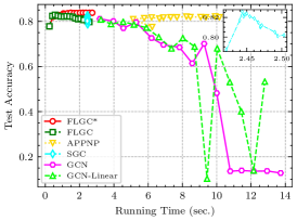
(a)

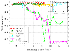
(b)

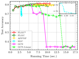
(c)

Figure 2: Classification accuracy vs. training time with varying propagation step on (a) Cora, (b) Citeseer, and (c) Pubmed datasets. We keep other hyperparameters fixed except for $K$ for each model so that running time is affected only by the propagation step. In the figures, each curve contains 15 points (i.e., 15 propagation steps) and each corresponds to the running time (x-axis) and test accuracy (y-axis) yielded by a specific $K$-hop model, where $K=\left[1,2,\cdots,15\right]$ and increases with running time. The insets indicate the zoom-up of SGC.

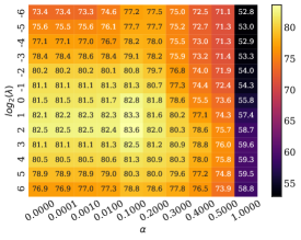
(a)

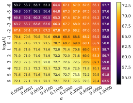
(b)

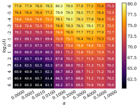
(c)

Figure 3: Effect of $\lambda$ and $\alpha$ on (a) Cora, (b) Citeseer, and (c) Pubmed datasets.

IV-A Results on Real-World Benchmarks

IV-A1 Dataset Description

We evaluate our proposed FLGCs on three standard citation network datasets available from the PyTorch Geometric library, including the Cora, Citeseer, and PubMed [39]. The summary of these datasets is reported in Table I. In these datasets, nodes correspond to documents, and edges correspond to citations; each node feature corresponds to the bag-of-words representation of the document and belongs to one of the academic topics [40]. Given a portion of nodes and their labeled categories, e.g., history and science, the task is to predict the category for other unlabeled nodes over the same graph.

IV-A2 Baselines and Setup

For citation network datasets, the proposed FLGCs compare against numerous SOTA graph neural network models, including the vanilla GCN [12], GAT [15], FastGCN [41], GIN [42], LNET, AdaLNet [43], DGI [44], SGC [20], MixHop [45], DropEdge [18], and G³NN [46]. For these models, we give their results reported in the corresponding literature. Moreover, we reproduce the vanilla GCN w/o non-linear activation (GCN or GCN-Linear), SGC, and APPNP [21]. In our reproduction, we follow the settings suggested in the corresponding papers. Specifically, we implement GCN and GCN-Linear using two-layer graph convolution each with $16$ hidden neurons, and apply an $L_{2}$ regularization with $\lambda=0.0005$ on trainable parameters. For APPNP, we adopt a two-layer MLP, each of which contains $64$ hidden neurons and $\lambda=0.005$. For a fair comparison, we discard other training tricks involved in backpropagation except for weight decay.

We implement two variants of our FLGC model with the PyTorch library, i.e., FLGC* indicates our method that uses our propagation mechanism and FLGC denotes our model that uses the SGC propagation. The hyper-parameters in our models are determined by a grid search among $\lambda=[2^{-8},2^{8}]$, $\alpha=[0,1]$, and $K=[0,20]$. We train and test all baselines with the same data splits and random seeds on an NVIDIA GTX 1080 Ti GPU, and report the average accuracy over $20$ runs. In our experiment, we provide three types of data splits, i.e., public splits as described in [39], random splits where training/validation/test sets are generated randomly with the same proportion as the public splits, and full splits where all remaining nodes are considered as the training set.

IV-A3 Comparison with SOTAs

Table II reports the classification accuracies of node classification with public splits. The results shown in the top part of Table II are collected from [12, 15, 41, 42, 43, 44, 20, 45, 18, 46] while the results shown in the middle part of Table II are reproduced in our experiment. It can be seen that our FLGC models consistently achieve large-margin outperformance across all datasets. Through a point-by-point comparison, FLGC improves upon SGC by a margin of $1.2\%$, $1.6\%$, and $2.6\%$ (absolute differences) on Cora, Citeseer, and Pubmed, respectively, while the margins improved by FLGC* upon APPNP are $1.5\%$, $2.8\%$, and $1.7\%$, respectively. Through a vertical comparison, FLGC* achieves $1.1\%$, $0.5\%$ and $1.9\%$ improvement over FLGC, respectively.

In Table III, we further report the comparison results using the random splits and full splits. We can observe that the proposed FLGCs collectively outperform the competitors in terms of average classification accuracy. It should be noted that our FLGCs tend to obtain a more stable result than other baselines because of their ability to offer closed-form solutions. In a nutshell, the above experiments demonstrate that our FLGC framework is capable of achieving the SOTA performance.

IV-A4 Running Time and Over-smoothing Analysis

Fig. 2 depicts the interaction between training time and classification accuracy. To ensure a fair comparison, all the training times are collected from the same hardware. In particular, the precomputation time of $\mathbf{H}$ is taken into account for SGC and FLGCs. We use fixed hyperparameters to train each model and let $K$ be the only variable increasing from $1$ to $15$. Thus, the running time of each model will definitely increase with $K$, and then will indirectly affect the test accuracy. Remarkably, GCN and linear GCN suffer from unstable performance when $K\geq 2$ because of over-smoothing. On the contrary, both FLGC and FLGC* are robust to the propagation steps. Especially, there is no significant over-smoothing effect in FLGC* across three figures, signifying the effectiveness of our propagation scheme. Also, it suggests that the residual connection is helpful to address the over-smoothing problem.

For a given graph, the training time of a graph model is positively associated with the propagation steps (or layers). Nonetheless, our FLGCs show a notable advantage over other methods (e.g., GCN and APPNP). Especially, it is almost no increase in the computation time using our multi-hop propagation scheme. Instead, such a strategy improves FLGC significantly, particularly with large $K$. Despite computation efficiency, SGC suffers from over-smoothing and its training relies on the optimizer and its parameter settings. In summary, our FLGC model achieves a good balance between classification accuracy and training time.

TABLE IV: Details of 24 UCI benchmark datasets.

Dataset	#classes	#instances	#features	#train	#test	Dataset	#classes	#instances	#features	#train	#test
air	3	359	64	37	322	appendicitis	2	106	7	12	94
ecoli	8	336	7	38	298	heart	2	270	13	27	243
iris	3	150	4	15	135	cleve	2	296	13	30	266
fertility	2	100	9	11	89	segmentation	7	210	18	21	189
wine	3	178	13	19	159	x8d5k	5	1000	8	100	900
wdbc	2	569	30	58	511	vote	2	435	16	44	391
haberman	3	306	3	32	274	wbc	2	683	9	69	614
spectf	2	267	44	28	239	WBC	2	683	9	69	614
cotton	6	356	21	37	319	breast	2	277	9	29	248
seeds	3	210	7	21	189	australian	2	690	14	70	620
glass	6	214	10	23	191	diabetes	2	768	8	78	690
zoo	7	101	16	13	88	dnatest	3	1186	180	120	1066

IV-A5 Impact of $\lambda$ and $\alpha$

We study the sensitivity of $\lambda$ and $\alpha$ of FLGC. As depicted in Fig. 3 (a)-(f), both $\lambda$ and $\alpha$ have a significant effect on the accuracy. Due to the difference in the neighborhood structure, the optimum of $\lambda$ and $\alpha$ will be varied for different datasets. Usually, a large $\lambda$ value tends to bring a compact model, while a small value increases the risk of over-fitting. For Cora and Citeseer datasets, a large $\lambda$ is desired by the FLGC models, while this value should be small on the Pubmed dataset. It should be noticed that FLGC* is equivalent to FLGC and the classic ridge regression classifier when $\alpha=0$ and $\alpha=1$, respectively. It can be seen that the best settings for this hyper-parameter is around $\alpha\in\left[0.01,0.2\right]$. The teleport probability $\alpha$ serves as a proportion showing to what extent original features contribute to the propagation. Our further analysis revealed the following tendencies: First, compared to the two endpoints ($\alpha=0$ and $\alpha=1$) in Fig. 3, FLGC improves the classic ridge regression with a significant margin. This means that structure information is pretty useful for the traditional linear model. Second, the original node features are helpful to improve FLGC, which makes it possible to aggregate higher hop neighbors.

IV-B Results on Regular Datasets

IV-B1 Dataset Description

To further explore the generalization ability of FLGCs, we conduct a series of experiences on $24$ widely-used regular classification datasets taken from the University of California at Irvine (UCI) repository. These datasets include a number of binary-class and multi-class classification problems. In the preprocessing, all datasets are scaled into the range of $[0,1]$ using the min-max standardization technique. For each dataset, we randomly take $10\%$ samples from each class as the labeled set and the rest $90\%$ as the unlabeled set. A detailed description of these datasets is provided in Table IV.

TABLE V: Semi-supervised classification accuracy on 24 UCI datasets. Best results are in bold.

Dataset	SS-ELM	TSVM	LapRLS	GCN-Linear	GCN	DropEdge	SGC	GCNII	APPNP	FLGC	FLGC*
air	76.23$\pm$4.08	80.19$\pm$3.65	76.09$\pm$6.08	90.09$\pm$4.09	90.12$\pm$3.80	86.43$\pm$4.13	78.94$\pm$3.71	89.16$\pm$2.53	90.31$\pm$4.17	90.65$\pm$2.89	91.02$\pm$3.44
ecoli	77.41$\pm$5.31	79.43$\pm$4.34	85.86$\pm$1.99	83.41$\pm$3.90	83.55$\pm$3.87	80.71$\pm$2.85	77.13$\pm$1.47	83.28$\pm$2.61	81.32$\pm$3.96	84.09$\pm$2.10	84.73$\pm$1.92
iris	80.19$\pm$4.26	92.56$\pm$3.67	91.93$\pm$3.34	91.63$\pm$4.63	90.81$\pm$4.89	88.81$\pm$5.95	88.59$\pm$6.29	92.67$\pm$2.05	91.41$\pm$3.49	96.30$\pm$0.66	96.81$\pm$0.47
Fertility	75.28$\pm$10.03	71.74$\pm$8.72	77.25$\pm$5.80	73.03$\pm$9.91	74.38$\pm$10.31	83.48$\pm$4.69	88.76$\pm$0.00	76.18$\pm$8.92	77.87$\pm$9.36	88.76$\pm$0.00	88.76$\pm$0.00
wine	79.53$\pm$7.66	94.09$\pm$2.10	95.13$\pm$2.12	93.08$\pm$1.57	93.14$\pm$1.14	90.44$\pm$2.00	91.13$\pm$4.50	93.33$\pm$2.69	91.64$\pm$2.22	94.03$\pm$1.69	94.28$\pm$1.47
wdbc	89.17$\pm$5.90	93.64$\pm$1.83	85.92$\pm$2.41	93.56$\pm$1.75	93.60$\pm$2.05	93.68$\pm$1.60	91.78$\pm$1.68	93.52$\pm$0.98	93.62$\pm$1.86	94.58$\pm$0.90	95.60$\pm$0.67
Haberman	71.73$\pm$2.44	62.57$\pm$5.73	70.02$\pm$3.15	70.51$\pm$2.15	70.40$\pm$2.83	67.96$\pm$4.15	73.72$\pm$0.00	70.88$\pm$2.05	69.71$\pm$2.63	73.72$\pm$0.00	73.72$\pm$0.00
SPECTF	77.41$\pm$1.83	74.33$\pm$3.41	49.77$\pm$4.59	77.24$\pm$2.55	78.49$\pm$1.93	76.99$\pm$4.24	79.50$\pm$0.00	79.50$\pm$0.00	78.58$\pm$2.07	79.50$\pm$0.00	79.50$\pm$0.00
CAR	74.18$\pm$3.00	86.46$\pm$2.19	83.78$\pm$1.20	79.36$\pm$1.18	85.52$\pm$1.23	82.77$\pm$1.80	73.89$\pm$0.73	85.40$\pm$1.10	85.03$\pm$1.17	78.91$\pm$0.78	78.96$\pm$0.84
cotton	60.64$\pm$4.00	78.10$\pm$3.24	76.10$\pm$3.90	74.83$\pm$3.12	75.45$\pm$3.26	71.25$\pm$4.43	72.88$\pm$2.05	75.49$\pm$2.03	75.86$\pm$2.30	73.70$\pm$5.70	78.24$\pm$4.37
Seeds	87.22$\pm$7.08	91.93$\pm$2.58	92.83$\pm$1.76	90.63$\pm$2.40	90.42$\pm$2.83	78.31$\pm$20.88	89.89$\pm$0.69	91.48$\pm$1.60	89.47$\pm$2.93	92.06$\pm$0.63	93.17$\pm$1.12
glass	64.26$\pm$7.54	77.16$\pm$4.27	73.58$\pm$4.79	78.74$\pm$4.18	77.85$\pm$4.09	56.39$\pm$20.35	71.47$\pm$5.92	79.63$\pm$3.20	76.34$\pm$5.79	74.55$\pm$5.49	74.87$\pm$5.47
zoo	78.78$\pm$10.07	98.58$\pm$1.24	97.03$\pm$1.99	92.59$\pm$3.57	92.82$\pm$2.65	85.06$\pm$4.34	91.06$\pm$3.12	92.59$\pm$3.41	92.24$\pm$2.94	93.06$\pm$3.30	93.06$\pm$1.11
appendicitis	81.44$\pm$5.92	75.11$\pm$11.76	72.55$\pm$5.83	80.43$\pm$7.86	80.32$\pm$7.81	81.17$\pm$5.81	82.34$\pm$2.29	82.66$\pm$7.93	81.49$\pm$6.83	83.19$\pm$6.86	83.30$\pm$5.69
heart	71.71$\pm$6.32	73.27$\pm$4.16	73.85$\pm$3.18	76.09$\pm$5.46	76.13$\pm$4.12	75.51$\pm$9.46	79.14$\pm$3.39	76.67$\pm$6.58	77.28$\pm$6.13	81.11$\pm$1.31	81.65$\pm$1.38
cleve	71.07$\pm$5.87	73.98$\pm$5.49	71.60$\pm$3.15	76.28$\pm$2.81	75.79$\pm$3.63	71.50$\pm$4.59	76.39$\pm$1.48	76.88$\pm$2.98	77.03$\pm$3.79	77.37$\pm$1.93	77.44$\pm$2.35
segmentation	55.63$\pm$5.85	76.06$\pm$6.44	80.61$\pm$5.02	76.98$\pm$2.91	75.98$\pm$3.55	69.21$\pm$7.27	71.32$\pm$3.03	78.20$\pm$3.84	74.66$\pm$3.31	76.51$\pm$4.13	79.10$\pm$4.16
X8D5K	94.33$\pm$4.29	100.0$\pm$0.0	100.0$\pm$0.0	100.0$\pm$0.0	100.0$\pm$0.0	100.0$\pm$0.0	100.0$\pm$0.0	100.0$\pm$0.0	100.0$\pm$0.0	100.0$\pm$0.0	100.00$\pm$0.00
vote	80.54$\pm$5.32	90.52$\pm$1.75	84.90$\pm$3.02	89.23$\pm$2.48	89.64$\pm$2.42	87.37$\pm$2.50	87.34$\pm$1.04	90.20$\pm$2.06	89.85$\pm$2.19	91.10$\pm$1.51	91.79$\pm$1.46
WBC	92.73$\pm$3.43	92.38$\pm$2.68	93.98$\pm$1.33	95.70$\pm$1.56	95.88$\pm$1.07	96.69$\pm$0.51	95.90$\pm$0.51	95.64$\pm$0.50	95.65$\pm$0.81	96.19$\pm$0.47	96.48$\pm$0.66
breast	69.96$\pm$3.86	63.47$\pm$4.85	71.73$\pm$2.52	66.25$\pm$4.18	66.90$\pm$4.05	71.13$\pm$3.29	70.97$\pm$0.00	67.50$\pm$3.13	68.79$\pm$3.07	72.10$\pm$1.41	73.35$\pm$1.49
austra	78.54$\pm$5.48	77.65$\pm$3.83	81.49$\pm$2.37	85.44$\pm$1.64	85.23$\pm$1.98	76.97$\pm$11.37	81.87$\pm$1.37	84.35$\pm$1.06	83.98$\pm$3.10	85.16$\pm$1.54	85.66$\pm$0.68
diabetes	69.93$\pm$2.96	66.75$\pm$2.75	70.69$\pm$1.55	68.13$\pm$0.92	69.10$\pm$1.05	67.13$\pm$1.81	65.01$\pm$0.87	70.09$\pm$1.13	69.10$\pm$1.50	69.31$\pm$1.55	69.48$\pm$1.10
dnatest	48.96$\pm$2.27	82.95$\pm$1.53	83.47$\pm$1.19	85.30$\pm$1.07	85.54$\pm$1.05	81.91$\pm$1.42	74.40$\pm$1.85	87.80$\pm$1.00	82.03$\pm$5.27	84.92$\pm$0.92	85.39$\pm$1.27
Average	75.29$\pm$5.20	81.37$\pm$3.84	80.84$\pm$3.01	82.86$\pm$3.16	83.21$\pm$3.15	80.04$\pm$5.39	81.39$\pm$1.92	83.88$\pm$2.64	83.05$\pm$3.37	84.62$\pm$1.91	85.27$\pm$1.71

TABLE VI: Summary of ranks computed by the Wilcoxon test. "$\shortuparrow$" denotes the method in the row improves the method of the column. "$\shortdownarrow$" indicates the method in the column improves the method of the row. The upper diagonal of level significance is 0.1 while the lower diagonal level of significance is 0.05.

	SS-ELM	TSVM	LapRLS	GCN-Linear	GCN	DropEdge	SGC	GCNII	APPNP	FLGC	FLGC*
SS-ELM	-	66.0 $\shortdownarrow$	54.0 $\shortdownarrow$	23.0 $\shortdownarrow$	18.0 $\shortdownarrow$	56.0 $\shortdownarrow$	15.0 $\shortdownarrow$	8.0 $\shortdownarrow$	10.0 $\shortdownarrow$	1.0 $\shortdownarrow$	1.0 $\shortdownarrow$
TSVM	234.0 $\shortuparrow$	-	136.0	74.0 $\shortdownarrow$	66.0 $\shortdownarrow$	157.0	142.0	48.0 $\shortdownarrow$	80.0 $\shortdownarrow$	53.0 $\shortdownarrow$	37.0 $\shortdownarrow$
LapRLS	246.0 $\shortuparrow$	140.0	-	110.0	100.0	167.0	146.0	74.0 $\shortdownarrow$	106.0	67.0 $\shortdownarrow$	41.0 $\shortdownarrow$
GCN-Linear	277.0 $\shortuparrow$	202.0	166.0	-	99.0	215.0 $\shortuparrow$	191.0	42.5 $\shortdownarrow$	135.5	41.5 $\shortdownarrow$	22.0 $\shortdownarrow$
GCN	282.0 $\shortuparrow$	210.0 $\shortuparrow$	176.0	177.0	-	231.0 $\shortuparrow$	197.0 $\shortuparrow$	48.0 $\shortdownarrow$	172.5	63.0	38.0 $\shortdownarrow$
DropEdge	244.0 $\shortuparrow$	119.0	109.0	61.0 $\shortdownarrow$	45.0 $\shortdownarrow$	-	101.0	34.0 $\shortdownarrow$	37.0 $\shortdownarrow$	13.0 $\shortdownarrow$	9.0 $\shortdownarrow$
SGC	285.0 $\shortuparrow$	134.0	130.0	85.0	79.0	175.0	-	65.5 $\shortdownarrow$	71.0 $\shortdownarrow$	5.0 $\shortdownarrow$	5.0 $\shortdownarrow$
GCNII	292.0 $\shortuparrow$	228.0 $\shortuparrow$	202.0	257.5 $\shortuparrow$	228.0 $\shortuparrow$	242.0 $\shortuparrow$	234.5 $\shortuparrow$	-	208.0 $\shortuparrow$	104.5	65.5 $\shortdownarrow$
APPNP	290.0 $\shortuparrow$	196.0	170.0	140.5	127.5	239.0 $\shortuparrow$	205.0 $\shortuparrow$	68.0 $\shortdownarrow$	-	46.0 $\shortdownarrow$	29.0 $\shortdownarrow$
FLGC	299.0 $\shortuparrow$	223.0 $\shortuparrow$	209.0$\shortuparrow$	235.5 $\shortuparrow$	214.0 $\shortuparrow$	263.0 $\shortuparrow$	295.0 $\shortuparrow$	195.5	230.0 $\shortuparrow$	-	5.0 $\shortdownarrow$
FLGC*	299.0 $\shortuparrow$	239.0 $\shortuparrow$	235.0 $\shortuparrow$	254.0 $\shortuparrow$	238.0 $\shortuparrow$	267.0 $\shortuparrow$	295.0 $\shortuparrow$	234.5 $\shortuparrow$	247.0 $\shortuparrow$	271.0 $\shortuparrow$	-

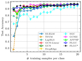
(a)

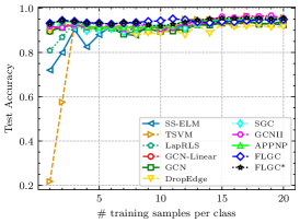
(b)

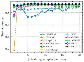
(c)

Figure 4: Test accuracy with different training samples per class on (a) Iris, (b) Wine, (c) WDBC datasets.

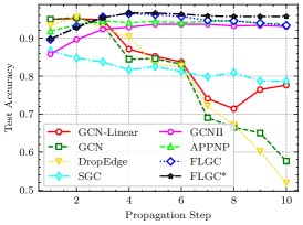
(a)

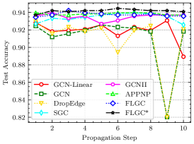
(b)

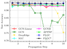
(c)

Figure 5: Over-smoothing effect on (a) Iris, (b) Wine, (c) WDBC datasets.

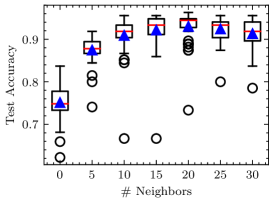
(a)

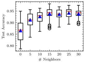
(b)

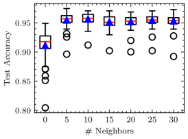
(c)

Figure 6: Effect of neighbor size on (a) Iris, (b) Wine, (c) WDBC datasets. We perform FLGC by fixing $\lambda=10^{-4}$, $K=5$, and $\alpha=0.1$ and varying $k\in\left\{0,5,10,15,20,25,30\right\}$. Noticed that $k=0$ means $\mathbf{A}=\mathbf{I}$ and thus only $\mathbf{X}$ is used. Each box indicates the statistic over $50$ independent runs and corresponding average value is denoted as a blue triangle.

IV-B2 Baselines and Setup

In this experiment, the selected baselines include GCN variants, i.e., GCN-Linear, GCN [12], DropEdge [18], SGC [20], GCNII [16], and APPNP [21], and classic semi-supervised classification models, i.e., SS-ELM [47], TSVM [48], and LapRLS [25]. There is no off-the-shelf structure in these regular datasets, thus, we construct $k$NN graphs [7, 26] for the representation of structured information. Specifically, we adopt the Euclidean distance to measure the similarity between sample pairs and choose top $k$ neighbors centered on a certain sample as its edges. To avoid hyper-parameter $k$, we empirically set it as $k=\left\lfloor\frac{N}{5C}\right\rfloor$.

IV-B3 Comparison with SOTAs and Statistical Test

In Table V, we provide the comparative results on the 24 UCI datasets. All the results are calculated by averaging $30$ independent runs. At the bottom of the table, we summarize the arithmetic mean accuracy over 24 datasets. Remarkably, our FLGC models consistently outperform not only the classic semi-supervised models but also the recent GCN variants. Specifically, FLGC* achieves the highest accuracy on $16$ out of $24$ datasets. On average, FLGC and FLGC* respectively obtain $84.62\pm 1.91$ and $85.27\pm 1.71$ accuracy across 24 datasets, which improve upon SGC and APPNP by margins of $3.23\%$ and $2.22\%$, respectively. Furthermore, we notice that GCN variants are generally superior to classic semi-supervised models even on the regular grid datasets. This is a valuable clue in designing semi-supervised models on regular datasets.

To further rank all baselines, we carry on a non-parametric statistical test on the results reported in Table V. To this end, we follow the suggestion posed by Garcia et al. [49] on adopting the Wilcoxon signed-ranks test to compute the sum of ranks for each pair of methods. Table VI shows the detailed statistical results. According to the exact critical value table of the Wilcoxon test, the critical values on $24$ datasets for a confidence level of $0.05$ and $0.1$ correspond to $81$ (lower diagonal) and $91$ ( upper diagonal), respectively. We can observe that our proposed FLGC* is significantly better than all the other competitors for different confidence levels, while the FLGC model performs equally to GCNII and GCN for the confidence level of $0.05$ and $0.1$, respectively. The results markedly demonstrate that our proposed FLGC models can generalize to the regular Euclidean data and can achieve promising performance.

IV-B4 Comparison w.r.t. Different Sizes of Training Samples

We conduct an experiment to compare the performance of baselines with varying labeled samples size. Fig. 4 (a)-(c) illustrate the comparative results on three selected datasets, i.e., Iris, Wine, and WDBC. We gradually increase the training samples per class from 1 to 20 and plot the test accuracy curves of $11$ competitive methods. It can be seen that both of our FLGC models show competitive performance w.r.t. the other baselines under different training sizes. Particularly, our methods remarkably outperform many baselines (e.g., SS-ELM, TSVM, and LapRLS) using all datasets when using an extremely small training size, e.g., only 1 labeled sample per class.

IV-B5 Study on Over-Smoothing

Fig. 5 (a)-(c) show the effect of the propagation step on the selected datasets. Several tendencies can be observed from the figures. Firstly, GCNII, APPNP, FLGC, and FLGC* face less risk of falling into the over-smoothing dilemma, while that occurs in the other methods. Secondly, linear GCN tends to outperform the nonlinear GCN on the selected datasets. A conceivable reason is that the nonlinear activation accelerates the speed of over-smoothing. Also, this is affected by the predefined graph structure. Thirdly, by adding initial residual, FLGC* benefits from the longer-range propagation, and thus significantly improves upon FLGC.

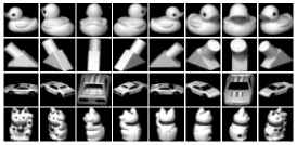
(a)

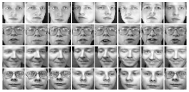
(b)

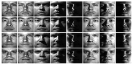
(c)

Figure 7: Sample images from (a) COIL20, (b) ORL, and (c) Extended Yale B.

TABLE VII: The clustering performance of different clustering models on Iris, Wine, and Yale datasets.

Datasets	Metric	K-Means	NMF	NCut	CAN	CLR	SSR	KMM	RRCSL	EGCSC	FLGC	FLGC*
Iris	ACC	0.797	0.636	0.586	0.573	0.846	0.686	0.817	0.873	0.940	0.953	0.960
	NMI	0.637	0.404	0.572	0.427	0.723	0.580	0.682	0.754	0.851	0.874	0.886
Wine	ACC	0.960	0.722	0.959	0.926	0.915	0.955	0.541	0.972	0.949	0.949	0.983
	NMI	0.862	0.447	0.881	0.780	0.732	0.848	0.361	0.881	0.820	0.820	0.928
Yale	ACC	0.472	0.339	0.511	0.521	0.509	0.593	0.442	0.600	0.515	0.546	0.630
	NMI	0.540	0.412	0.561	0.549	0.582	0.584	0.506	0.631	0.558	0.557	0.657

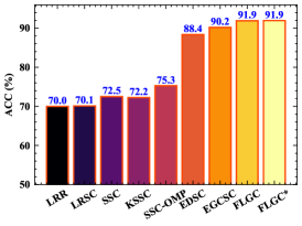
(a)

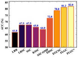
(b)

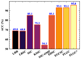
(c)

Figure 8: Clustering ACC (in %) on the (a) COIL20, (b) ORL, and (c) Extended Yale B datasets. Different colors indicate different methods. The height of the bars indicates the clustering ACC, so the higher the better.

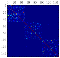
(a)

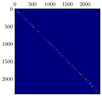
(b)

Figure 9: Affinity matrix obtained by FLGC* for (a) Iris and (b) Extended Yale B datasets.

TABLE VIII: Clustering results of the robustness experiments on the Extended Yale B dataset.

Noise Type	Noise Intensity	ACC				NMI
		EDSC	EGCSC	FLGC	FLGC*	EDSC	EGCSC	FLGC	FLGC*
Gaussian	$\sigma^{2}=0.01$	0.853	0.863	0.863	0.901	0.897	0.881	0.881	0.919
	$\sigma^{2}=0.05$	0.838	0.830	0.830	0.891	0.884	0.855	0.855	0.906
	$\sigma^{2}=0.1$	0.472	0.748	0.748	0.824	0.748	0.780	0.780	0.866
	$\sigma^{2}=0.2$	0.680	0.643	0.643	0.774	0.774	0.710	0.710	0.813
Salt & Pepper	$p=0.01$	0.845	0.891	0.891	0.908	0.886	0.901	0.901	0.922
	$p=0.05$	0.842	0.862	0.862	0.896	0.885	0.883	0.883	0.913
	$p=0.1$	0.843	0.847	0.847	0.894	0.885	0.870	0.870	0.912
	$p=0.2$	0.838	0.826	0.826	0.877	0.881	0.850	0.850	0.901

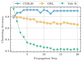
(a)

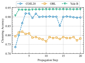
(b)

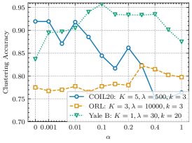
(c)

Figure 10: Effect of propagation step on the clustering accuracy of (a) FLGC and (b) FLGC*. (c) The influence of $\alpha$ on three benchmarks.

IV-B6 Effect of the Neighborhood Size

We aim to further explore the effect of the predefined graph structure on the classification performance of our FLGC. Fig. 6 shows the tendency of accuracy varied with neighborhood sizes. When $k=0$, meaning $\mathbf{P}=\mathbf{I}$, FLGC performs identically to a ridge regression classifier. At this point, FLGC’s performance becomes more unstable and worse than that considered neighborhood information. This demonstrates that a pairwise relationship defines the intrinsic structure of regular data. Different from real-word graph data, however, the predefined edges (i.e., $k$NN graph) cannot perfectly describe such structures. As a result, the performance of FLGC varies with neighborhood sizes. Empirically, a large neighborhood leads to more performance improvement since that enlarges the first-order receptive field. However, a too large neighborhood size will inevitably degrade the performance because of the increased risk of noisy edges and over-smoothing. It is still an open problem to find an optimum neighborhood size.

V Experiments of Clustering

In this section, we extensively evaluate our proposed unsupervised FLGC on several challenging clustering benchmarks and compare it with many previous clustering models.

V-A Dataset Description

Except for two simple UCI datasets (i.e., Iris and Wine), we add four challenging image clustering benchmarks for performance comparison, i.e., COIL20 object image dataset and Yale, Extended Yale B, and ORL face image datasets. The COIL20 dataset contains $1,440$ gray-scale image samples with a spatial size of $32\times 32$ and consists of $20$ distinct objects, e.g., duck, cat, and car models. The ORL dataset is composed of $400$ human face images, with $40$ subjects each having $10$ samples. Following [50], we down-sampled the original face images from $112\times 92$ to $32\times 32$. The Yale and Extended Yale B datasets are popular benchmarks for subspace clustering. The former includes $165$ face images collected from $15$ individuals. The latter database is more challenging than the former because it contains $2,432$ images of $38$ human subjects acquired under different poses and illumination conditions. The resolution of the two face databases is scaled to $32\times 32$ and $42\times 48$, respectively. Some selected sample images from COIL20, ORL, and Extended Yale B are illustrated in Fig. 7.

V-B Baselines and Setup

We divide our experiment into two parts. In the first part, we aim to evaluate our methods on three small and simple datasets, i.e., Iris, Wine, and Yale. This part follows the settings suggested in [51]. We compare our method with the following baselines: K-Means, NMF [52], Normalized Cuts (NCut) [53], CAN [54], CLR [55], SSR [56], K-Multiple-Means (KMM) [57], EGCSC [7], and RRCSL [51]. Similar to Section IV, we use FLGC* to denote our method with the initial residual. In the second part, we conduct experiments on three challenging image datasets (i.e., COIL20, ORL, and Extended Yale B). The baselines that we compare FLGCs with in this part include Low Rank Representation (LRR) [58], LRSC [34], SSC [24], KSSC [59], SSC by Orthogonal Matching Pursuit (SSC-OMP) [60], EDSC [36], and EGCSC [7]. We follow the experiment setups reported in [50]. For our FLGC, we search for the optimum parameter setting among $\lambda\in\left[1,10^{4}\right]$, $K\in\left[1,20\right]$, $\alpha\in\left[0,1\right]$, and a $k$NN graph of $k=\left\lfloor\frac{N}{5C}\right\rfloor$.

Two popular metrics are utilized to quantify the performance of the clustering methods, including clustering Accuracy (ACC) and Normalized Mutual Information (NMI) [7, 51]. Specifically, both metrics range in $[0,1]$, and the higher score the more accurate clustering result.

V-C Quantitative and Qualitative Results

Table VII gives the quantitative comparison of different clustering models on three small datasets. We can observe that our FLGC models consistently achieve superior ACC and NMI with significant margins compared with many existing clustering models. Specifically, FLGC* obtains $0.960$ and $0.983$ ACC on Iris and Wine datasets, respectively, outperforming the advanced RRCSL ($0.873$ and $0.972$) and KMM ($0.817$ and $0.541$) by large margins. In Fig. 8, we provide a visual comparison of the clustering performance on the three challenging datasets. The results reveal that the proposed FLGC models can markedly improve many self-expressiveness-based clustering models. As an extension of subspace clustering, our unsupervised FLGC reduces the intra-class variations through neighborhood propagation, making it more robust to find the inherent subspace structure among data. Taking Iris and Extended Yale B datasets as examples, we visualize the affinity matrices yielded by FLGC*, as shown in Fig. 9. The visualizations exhibit distinctly block-diagonal structures, which are highly close to the corresponding ground truths.

V-D Analysis of Robustness

To analyze the robustness of FLGCs, we conduct experiments to compare the clustering performance under different noise conditions. Specifically, we adopt a Gaussian noise and a salt-and-pepper noise to corrupt images. The variance $\sigma^{2}$ of the Gaussian noise and the proportion of corrupted pixels $p$ by the salt and pepper noise are treated as the intensity of noise. We test our method with different intensities of 0.01, 0.05, 0.1, and 0.2. It can be observed from Table VIII, our FLGC* is more robust to noise than other methods. This superiority is benefited from the graph structure, as well as the initial residual propagation scheme. FLGC and EGCSC have the same performance which is because FLGC obtains the best performance when $K=1$, and FLGC degrades into SGCSC at this point. Compared with EDSC, the other three methods show lower sensitivity to noise, demonstrating the robustness of the graph convolution.

V-E Influence of $K$ and $\alpha$

To study the effect of over-smoothing, we show clustering accuracy under different propagation steps on the COIL20, ORL, and Extended Yale B datasets, given in Fig. 10 (a) and (b). We find that FLGC* (Fig. 10 (a)) is robust to large propagation steps since its performance is almost unaffected by a large $K$ on the Extended Yale B dataset. In comparison, the accuracy obtained by FLGC drops about 0.70 in terms of ACC for $K=20$. This robustness to large propagation step further demonstrates that the initial features are crucial for regular data. This conclusion is further supported in Fig. 10 (c), where the clustering ACC tends to be increased by large $\alpha$ for the ORL and Extended Yale B datasets. It should be noticed that the structure information shows a higher contribution than initial features for the COIL20 datasets. A conceivable reason is that the samples within COIL20 have a strong inter-class difference, which results in a more accurate structure.

VI Conclusions

In this paper, we have presented a unified and simple graph convolutional framework, i.e., fully linear graph convolution networks, which incorporates multi-hop neighborhood aggregation into classic linear models to further simplify the training, applying, and implementing of GCN. Technically, we train FLGC by computing a global optimal closed-form solution, resulting in efficient computation. Also, based on the framework, we developed a semi-supervised FLGC and an unsupervised FLGC for semi-supervised node classification tasks and unsupervised clustering tasks, respectively. Furthermore, we showed that FLGC acts as a generalization of traditional linear models on the non-Euclidean data. In comparison with existing approaches, our FLGCs achieved superior performance across real-word graphs and regular grid data concurrently. The success of our FLGC establishes a connection between GCN and classic linear models. Future work may include exploring more scalable linear models to deal with large-scale graph, inductive learning, and extending FLGC to different GCNs.

Acknowlegment

The authors would like to thank the anonymous reviewers for their constructive suggestions and criticisms.

References

- [1] Z. Zhang, P. Cui, and W. Zhu, “Deep learning on graphs: A survey,” IEEE Transactions on Knowledge and Data Engineering, pp. 1–1, 2020.
- [2] J. Zhou, G. Cui, Z. Zhang, C. Yang, Z. Liu, and M. Sun, “Graph neural networks: A review of methods and applications,” CoRR, vol. abs/1812.08434, 2018.
- [3] Q. Li, Z. Han, and X.-M. Wu, “Deeper insights into graph convolutional networks for semi-supervised learning,” in Thirty-Second AAAI Conference on Artificial Intelligence, 2018.
- [4] Z. Wu, S. Pan, F. Chen, G. Long, C. Zhang, and P. S. Yu, “A comprehensive survey on graph neural networks,” IEEE Transactions on Neural Networks and Learning Systems, pp. 1–21, 2020.
- [5] W. Fan, Y. Ma, Q. Li, Y. He, E. Zhao, J. Tang, and D. Yin, “Graph neural networks for social recommendation,” in The World Wide Web Conference, ser. WWW ’19, 2019, pp. 417–426.
- [6] F. Monti, D. Boscaini, J. Masci, E. Rodola, J. Svoboda, and M. M. Bronstein, “Geometric deep learning on graphs and manifolds using mixture model cnns,” in Proceedings of the IEEE Conference on Computer Vision and Pattern Recognition (CVPR), July 2017.
- [7] Y. Cai, Z. Zhang, Z. Cai, X. Liu, X. Jiang, and Q. Yan, “Graph convolutional subspace clustering: A robust subspace clustering framework for hyperspectral image,” IEEE Transactions on Geoscience and Remote Sensing, vol. 59, no. 5, pp. 4191–4202, 2021.
- [8] Y. Ding, X. Zhao, Z. Zhang, W. Cai, and N. Yang, “Multiscale graph sample and aggregate network with context-aware learning for hyperspectral image classification,” IEEE Journal of Selected Topics in Applied Earth Observations and Remote Sensing, vol. 14, pp. 4561–4572, 2021.
- [9] M. Gasse, D. Chetelat, N. Ferroni, L. Charlin, and A. Lodi, “Exact combinatorial optimization with graph convolutional neural networks,” in Advances in Neural Information Processing Systems, vol. 32. Curran Associates, Inc., 2019, pp. 15 580–15 592.
- [10] B. Wilder, E. Ewing, B. Dilkina, and M. Tambe, “End to end learning and optimization on graphs,” in Advances in Neural Information Processing Systems, H. Wallach, H. Larochelle, A. Beygelzimer, F. d'Alché-Buc, E. Fox, and R. Garnett, Eds., vol. 32, 2019, pp. 4672–4683.
- [11] M. Defferrard, X. Bresson, and P. Vandergheynst, “Convolutional neural networks on graphs with fast localized spectral filtering,” in Proceedings of the 30th International Conference on Neural Information Processing Systems, ser. NIPS’16. Red Hook, NY, USA: Curran Associates Inc., 2016, pp. 3844–3852.
- [12] T. N. Kipf and M. Welling, “Semi-supervised classification with graph convolutional networks,” in 5th International Conference on Learning Representations, ICLR 2017, Toulon, France, April 24-26, 2017, Conference Track Proceedings, 2017.
- [13] W. L. Hamilton, R. Ying, and J. Leskovec, “Inductive representation learning on large graphs,” in Proceedings of the 31st International Conference on Neural Information Processing Systems, ser. NIPS’17. Red Hook, NY, USA: Curran Associates Inc., 2017, pp. 1025–1035.
- [14] Y. Ding, X. Zhao, Z. Zhang, W. Cai, and N. Yang, “Graph sample and aggregate-attention network for hyperspectral image classification,” IEEE Geoscience and Remote Sensing Letters, pp. 1–5, 2021, doi: 10.1109/LGRS.2021.3062944.
- [15] P. Veličković, G. Cucurull, A. Casanova, A. Romero, P. Liȯ, and Y. Bengio, “Graph attention networks,” in International Conference on Learning Representations, 2018.
- [16] Z. W. Ming Chen, B. D. Zengfeng Huang, and Y. Li, “Simple and deep graph convolutional networks,” in Proceedings of the 37th International Conference on Machine Learning, 2020.
- [17] W. Feng, J. Zhang, Y. Dong, Y. Han, H. Luan, Q. Xu, Q. Yang, E. Kharlamov, and J. Tang, “Graph random neural networks for semi-supervised learning on graphs,” in Advances in Neural Information Processing Systems, H. Larochelle, M. Ranzato, R. Hadsell, M. F. Balcan, and H. Lin, Eds., vol. 33. Curran Associates, Inc., 2020, pp. 22 092–22 103.
- [18] Y. Rong, W. Huang, T. Xu, and J. Huang, “Dropedge: Towards deep graph convolutional networks on node classification,” in International Conference on Learning Representations, 2019.
- [19] T. Zhao, Y. Liu, L. Neves, O. Woodford, M. Jiang, and N. Shah, “Data augmentation for graph neural networks,” in The Thirty-Fifth AAAI Conference on Artificial Intelligence, 2021.
- [20] F. Wu, A. Souza, T. Zhang, C. Fifty, T. Yu, and K. Weinberger, “Simplifying graph convolutional networks,” in International Conference on Machine Learning, 2019, pp. 6861–6871.
- [21] J. Klicpera, A. Bojchevski, and S. Günnemann, “Predict then propagate: Graph neural networks meet personalized pagerank,” in International Conference on Learning Representations (ICLR), 2019.
- [22] L. Page, S. Brin, R. Motwani, and T. Winograd, “The pagerank citation ranking: Bringing order to the web.” Technical Report 1999-66, November 1999, previous number = SIDL-WP-1999-0120.
- [23] S. An, W. Liu, and S. Venkatesh, “Face recognition using kernel ridge regression,” in 2007 IEEE Conference on Computer Vision and Pattern Recognition, 2007, pp. 1–7.
- [24] E. Elhamifar and R. Vidal, “Sparse subspace clustering: Algorithm, theory, and applications,” IEEE Transactions on Pattern Analysis and Machine Intelligence, vol. 35, no. 11, pp. 2765–2781, Nov 2013.
- [25] M. Belkin, P. Niyogi, and V. Sindhwani, “Manifold regularization: A geometric framework for learning from labeled and unlabeled examples,” Journal of machine learning research, vol. 7, no. Nov, pp. 2399–2434, 2006.
- [26] Y. Cai, Z. Zhang, Z. Cai, X. Liu, and X. Jiang, “Hypergraph-structured autoencoder for unsupervised and semisupervised classification of hyperspectral image,” IEEE Geoscience and Remote Sensing Letters, pp. 1–5, 2021, doi: 10.1109/LGRS.2021.3054868.
- [27] M. Yin, J. Gao, and Z. Lin, “Laplacian regularized low-rank representation and its applications,” IEEE Transactions on Pattern Analysis and Machine Intelligence, vol. 38, no. 3, pp. 504–517, March 2016.
- [28] J. Gu, Z. Wang, J. Kuen, L. Ma, A. Shahroudy, B. Shuai, T. Liu, X. Wang, G. Wang, J. Cai, and T. Chen, “Recent advances in convolutional neural networks,” Pattern Recognition, vol. 77, pp. 354–377, 2018.
- [29] Y. Cai, X. Liu, and Z. Cai, “Bs-nets: An end-to-end framework for band selection of hyperspectral image,” IEEE Transactions on Geoscience and Remote Sensing, vol. 58, no. 3, pp. 1969–1984, 2020.
- [30] R. Hang, Q. Liu, H. Song, Y. Sun, F. Zhu, and H. Pei, “Graph regularized nonlinear ridge regression for remote sensing data analysis,” IEEE Journal of Selected Topics in Applied Earth Observations and Remote Sensing, vol. 10, no. 1, pp. 277–285, 2017.
- [31] P. Ghamisi, E. Maggiori, S. Li, R. Souza, Y. Tarablaka, G. Moser, A. De Giorgi, L. Fang, Y. Chen, M. Chi, S. B. Serpico, and J. A. Benediktsson, “New frontiers in spectral-spatial hyperspectral image classification: The latest advances based on mathematical morphology, markov random fields, segmentation, sparse representation, and deep learning,” IEEE Geoscience and Remote Sensing Magazine, vol. 6, no. 3, pp. 10–43, Sep. 2018.
- [32] Y. LeCun, Y. Bengio, and G. Hinton, “Deep learning,” Nature, vol. 521, no. 7553, pp. 436–444, 2015.
- [33] Y. Cai, Z. Zhang, Q. Yan, D. Zhang, and M. J. Banu, “Densely connected convolutional extreme learning machine for hyperspectral image classification,” Neurocomputing, 2020, doi:10.1016/j.neucom.2020.12.064.
- [34] R. Vidal and P. Favaro, “Low rank subspace clustering (lrsc),” Pattern Recognition Letters, vol. 43, pp. 47 – 61, 2014, iCPR2012 Awarded Papers.
- [35] K. He, X. Zhang, S. Ren, and J. Sun, “Deep residual learning for image recognition,” in The IEEE Conference on Computer Vision and Pattern Recognition (CVPR), June 2016.
- [36] Pan Ji, M. Salzmann, and Hongdong Li, “Efficient dense subspace clustering,” in IEEE Winter Conference on Applications of Computer Vision, March 2014, pp. 461–468.
- [37] M. Zhu, X. Wang, C. Shi, H. Ji, and P. Cui, “Interpreting and unifying graph neural networks with an optimization framework,” arXiv preprint arXiv:2101.11859, 2021.
- [38] T. N. Kipf and M. Welling, “Variational graph auto-encoders,” arXiv preprint arXiv:1611.07308, 2016.
- [39] P. Sen, G. Namata, M. Bilgic, L. Getoor, B. Galligher, and T. Eliassi-Rad, “Collective classification in network data,” AI magazine, vol. 29, no. 3, pp. 93–93, 2008.
- [40] Z. Yang, W. Cohen, and R. Salakhudinov, “Revisiting semi-supervised learning with graph embeddings,” in International conference on machine learning. PMLR, 2016, pp. 40–48.
- [41] J. Chen, T. Ma, and C. Xiao, “Fastgcn: Fast learning with graph convolutional networks via importance sampling,” in International Conference on Learning Representations, 2018.
- [42] K. Xu, W. Hu, J. Leskovec, and S. Jegelka, “How powerful are graph neural networks?” in International Conference on Learning Representations, 2018.
- [43] R. Liao, Z. Zhao, R. Urtasun, and R. S. Zemel, “Lanczosnet: Multi-scale deep graph convo-lutional networks,” in 7th International Conference on Learning Representations, ICLR 2019, 2019.
- [44] P. Velickovic, W. Fedus, W. L. Hamilton, P. Liò, Y. Bengio, and R. D. Hjelm, “Deep graph infomax.” in ICLR (Poster), 2019.
- [45] S. Abu-El-Haija, B. Perozzi, A. Kapoor, N. Alipourfard, K. Lerman, H. Harutyunyan, G. Ver Steeg, and A. Galstyan, “Mixhop: Higher-order graph convolutional architectures via sparsified neighborhood mixing,” in international conference on machine learning. PMLR, 2019, pp. 21–29.
- [46] J. Ma, W. Tang, J. Zhu, and Q. Mei, “A flexible generative framework for graph-based semi-supervised learning,” in 33rd Conference on Neural Information Processing Systems (NeurIPS 2019), 2019.
- [47] G. Huang, S. Song, J. N. D. Gupta, and C. Wu, “Semi-supervised and unsupervised extreme learning machines,” IEEE Transactions on Cybernetics, vol. 44, no. 12, pp. 2405–2417, Dec 2014.
- [48] T. Joachims, “Transductive inference for text classification using support vector machines,” in ICML, vol. 99, 1999, pp. 200–209.
- [49] S. Garcia and F. Herrera, “An extension on“statistical comparisons of classifiers over multiple data sets”for all pairwise comparisons,” Journal of machine learning research, vol. 9, no. Dec, pp. 2677–2694, 2008.
- [50] P. Ji, T. Zhang, H. Li, M. Salzmann, and I. Reid, “Deep subspace clustering networks,” in Advances in Neural Information Processing Systems 30, I. Guyon, U. V. Luxburg, S. Bengio, H. Wallach, R. Fergus, S. Vishwanathan, and R. Garnett, Eds. Curran Associates, Inc., 2017, pp. 24–33.
- [51] Q. Wang, R. Liu, M. Chen, and X. Li, “Robust rank-constrained sparse learning: A graph-based framework for single view and multiview clustering,” IEEE Transactions on Cybernetics, pp. 1–12, 2021, doi: 10.1109/TCYB.2021.3067137.
- [52] D. D. Lee and H. S. Seung, “Learning the parts of objects by non-negative matrix factorization,” Nature, vol. 401, no. 6755, pp. 788–791, 1999.
- [53] J. Shi and J. Malik, “Normalized cuts and image segmentation,” IEEE Transactions on pattern analysis and machine intelligence, vol. 22, no. 8, pp. 888–905, 2000.
- [54] F. Nie, X. Wang, and H. Huang, “Clustering and projected clustering with adaptive neighbors,” in Proceedings of the 20th ACM SIGKDD international conference on Knowledge discovery and data mining, 2014, pp. 977–986.
- [55] F. Nie, X. Wang, M. Jordan, and H. Huang, “The constrained laplacian rank algorithm for graph-based clustering,” in Proceedings of the AAAI conference on artificial intelligence, vol. 30, no. 1, 2016.
- [56] J. Huang, F. Nie, and H. Huang, “A new simplex sparse learning model to measure data similarity for clustering,” in Twenty-Fourth International Joint Conference on Artificial Intelligence, 2015.
- [57] F. Nie, C.-L. Wang, and X. Li, “K-multiple-means: A multiple-means clustering method with specified k clusters,” in Proceedings of the 25th ACM SIGKDD International Conference on Knowledge Discovery & Data Mining, 2019, pp. 959–967.
- [58] G. Liu, Z. Lin, S. Yan, J. Sun, Y. Yu, and Y. Ma, “Robust recovery of subspace structures by low-rank representation,” IEEE transactions on pattern analysis and machine intelligence, vol. 35, no. 1, pp. 171–184, 2012.
- [59] V. M. Patel and R. Vidal, “Kernel sparse subspace clustering,” in 2014 ieee international conference on image processing (icip). IEEE, 2014, pp. 2849–2853.
- [60] C. You, D. Robinson, and R. Vidal, “Scalable sparse subspace clustering by orthogonal matching pursuit,” in Proceedings of the IEEE conference on computer vision and pattern recognition, 2016, pp. 3918–3927.