On the Spontaneous Dynamics of Synaptic Weights in Stochastic Models with Pair-Based STDP

Abstract.

We investigate spike-timing dependent plasticity (STPD) in the case of a synapse connecting two neural cells. We develop a theoretical analysis of several STDP rules using Markovian theory. In this context there are two different timescales, fast neural activity and slower synaptic weight updates. Exploiting this timescale separation, we derive the long-time limits of a single synaptic weight subject to STDP. We show that the pairing model of presynaptic and postsynaptic spikes controls the synaptic weight dynamics for small external input, on an excitatory synapse. This result implies in particular that mean-field analysis of plasticity may miss some important properties of STDP. Anti-Hebbian STDP seems to favor the emergence of a stable synaptic weight, but only for high external input. In the case of inhibitory synapse the pairing schemes matter less, and we observe convergence of the synaptic weight to a non-null value only for Hebbian STDP. We extensively study different asymptotic regimes for STDP rules, raising interesting questions for future works on adaptative neural networks and, more generally, on adaptive systems.

1. Introduction

Understanding brain’s learning and memory is a challenging topic combining a large spectrum of research fields ranging from neurobiology to applied mathematics. Neural networks, through the dynamics of their connections, are able to store complex patterns over long periods of time, and as such are good candidates for the establishment of memory. In particular, the intensity $\displaystyle W$ of the connection between two neurons, the synaptic weight, is seen as an essential building block to explain learning and memory formation [39].

Synaptic plasticity, processes that can modify the synaptic weight, is a complex mechanism [8], but general principles have been inferred from experimental data and used for a long time in computational models.

Spike-timing dependent plasticity (STDP) gathers plasticity processes that depends on the timing of pre-synaptic and post-synaptic spiking activity. Many experimental protocols has been developed to study STDP: most use sequences of spikes pairing from either side of a specific synapse are presented, at a certain frequency and with a certain delay, see [10].

Experiments show that long-term synaptic plasticity is characterized by the coexistence of two different timescales. Membrane potential and pre/post-synaptic interspike intervals evolve on the order of several milliseconds, see [13]. Synaptic weights $\displaystyle W$ change on a slower timescale ranging from seconds to minutes before observing an effect of an STDP protocol on the synaptic weights. For this reason, a slow-fast approximation is proposed to analyze the associated mathematical models of synaptic plasticity. The analysis of slow-fast limits for a general class of STDP models is detailed in [30, 31, 29].

Computational models of synaptic plasticity have also used similar scaling principles, see [20, 32, 21, 35].

In pair-based models, the synaptic weight updates depend only on $\displaystyle\Delta t{=}t_{\rm post}-t_{\rm pre}$ for a subset of instants of pre/post-synaptic spikes $\displaystyle t_{\rm pre}/t_{\rm post}$.

Hebbian STDP plasticity occur when

• a pre-post pairing, i.e., $\displaystyle t_{\rm pre}{<}t_{\rm post}$ leads to an increase of the synaptic weight value (potentiation), which translates into $\displaystyle\Delta W{>}0$;

• a post-pre pairing, $\displaystyle t_{\rm post}{<}t_{\rm pre}$, leads to a smaller synaptic weight (depression), and therefore $\displaystyle\Delta W{<}0$.

Hebbian STDP has been observed at many different synapses [3, 10] and is extensively studied in computational models [20, 32, 21, 35, 19, 36, 12, 6, 37, 38, 16].

Other types of polarity have been observed experimentally, they are often neglected in theoretical studies of STDP. For example, Anti-Hebbian STDP follows the opposite principles, whereby pre-post pairings lead to depression, and post-pre pairings to potentiation. Such plasticities were observed experimentally in the striatum, see [11, 34]. Different types of STDP rules were analyzed in [33, 7, 37, 41, 34, 4].

The context, in general, is a single neuron receiving a large number of excitatory inputs subject to STDP, leading to a Fokker-Plank approach [35, 36, 6]. In particular, the importance of a single pairing is diluted over the large number of inputs in the mean-field limit, whereas by definition STDP relies on the repetition of such correlated pairings.

The use of the pre-/postsynaptic spike correlation function [20, 19, 12] was used to study the influence of STDP with high correlated inputs. However, this method relies on the assumption that all pairs of pre- and postsynaptic spikes impact the synaptic weight update. Several studies have questioned this hypothesis [18, 25, 26], and its influence on the synaptic weight dynamics has not been discussed in theoretical works, except in [6].

Finally, most studies focus on excitatory inputs, whereas inhibitory synapses also exhibit STDP [17, 10], but few theoretical works exist [24].

Here we develop a theoretical study of a large class of rules, for a system with two neurons and a single synapse. This simple setting is used to test the influence of STDP on an excitatory and an inhibitory synapse, for three different classes of pairing interactions leading to an extensive categorization of the different dynamics. We show in particular that several interesting properties of the synaptic weight dynamics are lost when using classical models with numerous excitatory inputs, leading to an underestimation of the role of STDP in learning systems.

2. Theoretical analysis

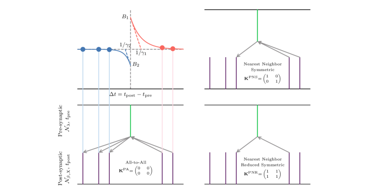
Figure 1. Synaptic Plasticity Kernels for Pair-Based Rules

2.1. Spiking neurons and Poisson processes

The spike train of the pre-synaptic neuron is represented by an homogeneous Poisson process $\displaystyle{\cal N}_{\lambda}$ with $\displaystyle\lambda{>}0$, where $\displaystyle\delta_{x}$ is the Dirac measure at $\displaystyle x{\in}\mathbb{R}$, then

$${\cal N}_{\lambda}{=}\sum_{n{\geq}1}\delta_{t_{{\rm pre},n}},\text{ with }0{\leq}t_{{\rm pre},1}\leq\cdots\leq t_{{\rm pre},n}\leq\cdots,$$

with $\displaystyle t_{pre/post}$ the pre- and postsynaptic spike times.

In particular $\displaystyle\mathbb{P}\left(\rule{0.0pt}{14.22636pt}{\cal N}_{\lambda}(t,t{+}\mathop{}\mathopen{}\mathrm{d}t){\neq}0\right){=}\lambda\mathop{}\mathopen{}\mathrm{d}t{+}o(\mathop{}\mathopen{}\mathrm{d}t)$.

We define a stochastic process $\displaystyle(X(t))$ following leaky-integrate dynamics:

1. It decays exponentially to $\displaystyle 0$ with a fixed exponential decay, set to $\displaystyle 1$.

2. It is incremented by the synaptic weight $\displaystyle W{>}0$ at each pre-synaptic spike, i.e. at each instant of $\displaystyle{\cal N}_{\lambda}$.

The firing mechanism of the postsynaptic neuron is driven by an activation function function $\displaystyle\beta$, when $\displaystyle X$ is $\displaystyle x$, the output neuron fires at rate $\displaystyle\beta(x)$. The sequence of instants of post-synaptic spikes $\displaystyle(t_{\textup{post},n})$ is a point process $\displaystyle{\cal N}_{\beta,X}$ on $\displaystyle\mathbb{R}_{+}$ such that

$$\mathbb{P}\left.\left(\rule{0.0pt}{14.22636pt}{\cal N}_{\beta,X}(t,t{+}\mathop{}\mathopen{}\mathrm{d}t){\neq}0\right|X(t){=}x\right){=}\beta(x)\mathop{}\mathopen{}\mathrm{d}t{+}o(\mathop{}\mathopen{}\mathrm{d}t).$$

The process represents the membrane potential of the postsynaptic neuron in the case of an excitatory synapse. For simplicity, we chose to differentiate between excitatory and inhibitory synapses at the level of the activation function, instead of allowing for negative $\displaystyle W$.

Indeed, for an excitatory synapse, the activation function $\displaystyle\beta(x){=}\nu{+}\beta x$ is used, $\displaystyle\nu$ is the rate of the external input to the post-synaptic neuron, it models external noise. For inhibitory synapses, we consider $\displaystyle\beta(x){=}\max(\nu{-}\beta x,0)$.

2.2. Pair-based STDP rules

We study an important implementation of STDP referred to as pair-based rules. For a pair $\displaystyle(t_{\rm pre},t_{\rm post})$ of instants of pre- and post-synaptic spikes, the synaptic weight update $\displaystyle\Delta W$ depends only on $\displaystyle\Delta t{=}t_{\rm post}{-}t_{\rm pre}$, as illustrated in Figure 1. Most of STDP experimental studies are based on such pairing protocols, where pre- and post-synaptic spikes are repeated with a fixed delay for a given number of evenly spaced pairings, see [26, 3, 10].

An important choice for the model is to decide which pairings to take into account in the plasticity update. A large choice of different schemes have been analyzed in the literature [26]. We have chosen to focus on three versions, that are summarized in Figure 1:

• PA: All-to-all pair-based model: all pairs of spikes are taken into account in the synaptic plasticity rule.

• PNS: Nearest neighbor symmetric model: whenever one neuron spikes, the synaptic weight is updated by only taking into account the last spike of the other neuron.

• PNR: Nearest neighbor symmetric reduced model: only consecutive pairs of spikes are used to update the synaptic weight.

The synaptic weight update is therefore composed of the sum over relevant spikes, of an kernel $\displaystyle\Phi(\Delta t)$ known as the plasticity curve, here we chose an exponential kernel, given by,

$$\Phi(\Delta t)=\begin{cases}B_{2}\exp(\gamma_{2}\Delta t)&\Delta t{<}0,\\ B_{1}\exp(-\gamma_{1}\Delta t)&\Delta t{>}0.\\ \end{cases}$$

where $\displaystyle B_{1},B_{2}{\in}\mathbb{R}$ represents the amplitude of the STDP and $\displaystyle\gamma_{1},\gamma_{2}>0$ the characteristic time of interaction, see Figure 1 (top).

All these pair-based rules can be represented by a system of the form

(1) $$\begin{cases}\mathop{}\mathopen{}\mathrm{d}X(t)&={-}X(t)\mathop{}\mathopen{}\mathrm{d}t+W(t{-})\mathcal{N}_{\lambda}(\mathop{}\mathopen{}\mathrm{d}t),\\ \mathop{}\mathopen{}\mathrm{d}Z_{1}(t)&={-}\gamma_{1}Z_{1}(t)\mathop{}\mathopen{}\mathrm{d}t\\ &\hskip 28.45274pt+(B_{1}-K_{1,1}Z_{1}(t{-}))\mathcal{N}_{\lambda}(\mathop{}\mathopen{}\mathrm{d}t)\\ &\hskip 28.45274pt-K_{1,2}Z_{1}(t{-})\mathcal{N}_{\beta,X}(\mathop{}\mathopen{}\mathrm{d}t),\\ \mathop{}\mathopen{}\mathrm{d}Z_{2}(t)&={-}\gamma_{2}Z_{2}(t)\mathop{}\mathopen{}\mathrm{d}t\\ &\hskip 28.45274pt+(B_{2}{-}K_{2,2}Z_{2}(t{-}))\mathcal{N}_{\beta,X}(\mathop{}\mathopen{}\mathrm{d}t)\\ &\hskip 28.45274pt-K_{2,1}Z_{2}(t{-})\mathcal{N}_{\lambda}(\mathop{}\mathopen{}\mathrm{d}t),\\ \mathop{}\mathopen{}\mathrm{d}W(t)&=Z_{1}(t{-})\mathcal{N}_{\beta,X}(\mathop{}\mathopen{}\mathrm{d}t)+Z_{2}(t{-})\varepsilon\mathcal{N}_{\lambda}(\mathop{}\mathopen{}\mathrm{d}t)\end{cases}$$

where $\displaystyle\gamma_{1},\gamma_{2}{>}0$, $\displaystyle B_{1},B_{2}{\in}\mathbb{R}$, $\displaystyle{\mathbf{K}}{=}(K_{ij},i,j{\in}\{1,2\}){\in}\{0,1\}^{4}$.

For the three pair-based STDP rules detailed, we have,

$${\mathbf{K}}^{\rm PA}{=}\begin{pmatrix}0&0\\ 0&0\end{pmatrix},\quad{\mathbf{K}}^{\rm PNS}{=}\begin{pmatrix}1&0\\ 0&1\end{pmatrix},\quad{\mathbf{K}}^{\rm PNR}{=}\begin{pmatrix}1&1\\ 1&1\end{pmatrix}.$$

Appendix B provides more details on the model and equations.

2.3. General formulation in a slow-fast system

We consider that the processes $\displaystyle(X(t))$ and $\displaystyle(Z_{1}(t),Z_{2}(t))$ evolve on a fast time scale $\displaystyle t{\mapsto}t/\varepsilon$ for some small $\displaystyle\varepsilon{>}0$. The increments of the variable $\displaystyle W$ are scaled with the parameter $\displaystyle\varepsilon$, so that the variation on a bounded time-interval is $\displaystyle O(1)$, $\displaystyle(W_{\varepsilon}(t))$ is described as the slow process.

An intuitive picture of approximation results used in this paper can be described as follows. For $\displaystyle\varepsilon$ small, on a short time interval, the slow process $\displaystyle(W_{\varepsilon}(t))$ is almost constant, and, due to its faster dynamics, the process $\displaystyle(X_{\varepsilon}(t),Z_{1,\varepsilon}(t),Z_{2,\varepsilon}(t))$ is “almost” at its equilibrium distribution associated to the current value of $\displaystyle W_{\varepsilon}(t){\approx}w$. This is also the equilibrium of the process $\displaystyle(X^{w}(t),Z_{1}^{w}(t),Z_{2}^{w}(t))$ such that

(2) $$\begin{cases}\mathop{}\mathopen{}\mathrm{d}X^{w}(t)\displaystyle&={-}X^{w}(t)\mathop{}\mathopen{}\mathrm{d}t+w\mathcal{N}_{\lambda}(\mathop{}\mathopen{}\mathrm{d}t),\\ \mathop{}\mathopen{}\mathrm{d}Z_{1}^{w}(t)\displaystyle&={-}\gamma Z_{1}^{w}(t)\mathop{}\mathopen{}\mathrm{d}t\\ &\hskip 28.45274pt+(B_{1}-K_{1,1}Z_{1}^{w}(t{-}))\mathcal{N}_{\lambda}(\mathop{}\mathopen{}\mathrm{d}t)\\ &\hskip 28.45274pt-K_{1,2}Z_{1}^{w}(t{-})\mathcal{N}_{\beta,X^{w}}(\mathop{}\mathopen{}\mathrm{d}t),\\ \mathop{}\mathopen{}\mathrm{d}Z_{2}^{w}(t)\displaystyle&={-}\gamma Z_{2}^{w}(t)\mathop{}\mathopen{}\mathrm{d}t\\ &\hskip 28.45274pt+(B_{2}-K_{2,2}Z_{2}^{w}(t{-}))\mathcal{N}_{\beta,X^{w}}(\mathop{}\mathopen{}\mathrm{d}t)\\ &\hskip 28.45274pt-K_{2,1}Z_{2}^{w}(t{-})\mathcal{N}_{\lambda}(\mathop{}\mathopen{}\mathrm{d}t).\end{cases}$$

Classical results on Markov systems imply that there is unique stationary distribution $\displaystyle\Pi_{w}^{\mathbf{K}}$ on‘ $\displaystyle\mathbb{R}_{+}{\times}\mathbb{R}^{2}$, for simplicity we will denote $\displaystyle\Pi_{w}^{\text{\rm PX}}{=}\Pi_{w}^{K^{\text{\rm PX}}}$, see [30]

Using averaging principle arguments, the asymptotic dynamic of $\displaystyle(W_{\varepsilon}(t))$ is given by the ODE,

(3) $$\displaystyle\frac{\mathop{}\mathopen{}\mathrm{d}w}{\mathop{}\mathopen{}\mathrm{d}t}(t) \displaystyle=\int_{\mathbb{R}_{+}{\times}\mathbb{R}^{2}}(\lambda z_{2}{+}\beta(x)z_{1})\Pi_{w(t)}^{\mathbf{K}}(\mathop{}\mathopen{}\mathrm{d}x,\mathop{}\mathopen{}\mathrm{d}z)$$

(4) $$\displaystyle=\mathbb{E}_{\Pi^{\mathbf{K}}_{w(t)}}\left[\lambda Z_{2}{+}\beta(X)Z_{1}\right].$$

A more rigorous development on this result is given in Appendix C.

LTD (Long Term Depression)	$\displaystyle\forall w_{0},$ $\displaystyle\displaystyle\lim_{t{\rightarrow}{+}\infty}w(t)=0$	$\displaystyle p_{+\infty}<p_{\text{\rm bif}}$ $\displaystyle p_{0}\geq p_{\text{\rm bif}}$ $\displaystyle p_{\text{\rm stable}}<p_{\text{\rm bif}}$
LTP (Long Term Potentiation)	$\displaystyle\forall w_{0},$ $\displaystyle\displaystyle\lim_{t{\rightarrow}{+}\infty}w(t)=+\infty$	$\displaystyle p_{+\infty}\geq p_{\text{\rm bif}}$ $\displaystyle p_{0}<p_{\text{\rm bif}}$ $\displaystyle p_{\text{\rm stable}}<p_{\text{\rm bif}}$
UNSTABLE Fixed Point	$\displaystyle\exists w_{\textup{eq}},\forall w_{0}{<}w_{\textup{eq}},$ $\displaystyle\displaystyle\lim_{t{\rightarrow}{+}\infty}w(t)=0$ and $\displaystyle\forall w_{0}{>}w_{\textup{eq}},$ $\displaystyle\displaystyle\lim_{t{\rightarrow}{+}\infty}w(t)=+\infty$	$\displaystyle p_{+\infty}\geq p_{\text{\rm bif}}$ $\displaystyle p_{0}\geq p_{\text{\rm bif}}$ $\displaystyle p_{\text{\rm stable}}<p_{\text{\rm bif}}$
STABLE Fixed Point	$\displaystyle\exists w_{\textup{eq}},$ $\displaystyle\forall w_{0},\displaystyle\lim_{t{\rightarrow}{+}\infty}w(t)=w_{\textup{eq}}$	$\displaystyle p_{+\infty}<p_{\text{\rm bif}}$ $\displaystyle p_{0}<p_{\text{\rm bif}}$ $\displaystyle p_{\text{\rm stable}}\geq p_{\text{\rm bif}}$
MULTIPLE Fixed Point	Other behaviors	Complementary set

Table 1. Different possible behaviors, theoretical definitions and numerical estimations

2.4. Computer simulations

To compare different dynamics, synapses and pairing schemes, we perform, for each set of parameters, independent simulations and from this array of dynamics we compute several variables:

• The probability of diverging to infinity, $\displaystyle p_{+\infty}{=}\mathbb{P}\left(W_{\varepsilon}(t){=}+\infty\right)$, approximated by the proportion of simulations where the synaptic weight goes above $\displaystyle w_{\text{\rm max}}$.

• The probability of converging to $\displaystyle 0$, $\displaystyle p_{0}{=}\mathbb{P}\left(W_{\varepsilon}(t){=}0\right)$, approximated by the proportion of simulations whose synaptic weight goes below $\displaystyle 0$.

• The probability to have a stable fixed point defined by the complementary probability $\displaystyle p_{\text{\rm st}}{=}1{-}p_{+\infty}{-}p_{0}$.

Five different asymptotic behaviors for $\displaystyle w$, solution of (3) are defined using analytical asymptotic properties in Table 1. We define numerical approximates of these possible behaviors, depending on the values of $\displaystyle p_{+\infty}$, $\displaystyle p_{0}$ and $\displaystyle p_{\text{\rm st}}$, and a fixed parameters $\displaystyle p_{\text{\rm bif}}$.

3. Results

Figure 2. All-to-all pair-based STDP for an excitatory synapse

In this framework, we study the asymptotic behavior of the dynamical system (3) for the three pair-based rules,

$$\frac{\mathop{}\mathopen{}\mathrm{d}w}{\mathop{}\mathopen{}\mathrm{d}t}(t){=}f^{\mathbf{K}}(w(t)),\text{ with }f^{\mathbf{K}}(w){\stackrel{{\scriptstyle\text{\rm def}.}}{{=}}}\mathbb{E}_{\Pi^{{\mathbf{K}}}_{w}}\left[\lambda Z_{2}{+}\beta(X)Z_{1}\right],$$

$\displaystyle{\mathbf{K}}{\in}\{{\rm PA},{\rm PNS},{\rm PNR}\}$.

We will show that the synaptic weight $\displaystyle w(t)$ usually end up having one of three different asymptotic behaviors, which all have a biological interpretation:

• Convergence of $\displaystyle w(t)$ towards $\displaystyle 0$, which corresponds the disconnection (or pruning) of the synapse: the presynaptic neuron loses its ability to influence the postsynaptic neuron.

• Divergence of $\displaystyle w(t)$ to infinity, leading an unstable system which, in a biological system, will be stopped by saturation mechanisms.

• Convergence to a non null value $\displaystyle w_{eq}$, resulting in self-sustained activity, i.e., pre- and postsynaptic activities coupled with STDP are sufficient to have a bounded stable synaptic weight.

3.1. Stability and divergence depends on the polarity of STDP

Starting with the all-to-all scheme for an excitatory synapse, i.e. $\displaystyle\beta(x){=}\nu{+}\beta x$, we have,

$$\frac{\mathop{}\mathopen{}\mathrm{d}w}{\mathop{}\mathopen{}\mathrm{d}t}(t)=f^{\text{\rm PA}}(w)=A^{\text{\rm PA}}_{0}{+}A^{\text{\rm PA}}_{1}w=A^{\text{\rm PA}}_{1}\left(w{-}w^{\text{\rm PA}}\right).$$

with

$$A^{\text{\rm PA}}_{0}\stackrel{{\scriptstyle\text{\rm def}.}}{{=}}\nu\lambda\left(\frac{B_{1}}{\gamma_{1}}{+}\frac{B_{2}}{\gamma_{2}}\right),\\ A^{\text{\rm PA}}_{1}\stackrel{{\scriptstyle\text{\rm def}.}}{{=}}\beta\lambda^{2}\left(\frac{B_{1}}{\gamma_{1}}{+}\frac{B_{2}}{\gamma_{2}}{+}\frac{B_{1}}{\lambda(1{+}\gamma_{1})}\right)\text{ and }\\ w^{\text{\rm PA}}\stackrel{{\scriptstyle\text{\rm def}.}}{{=}}{-}A^{\text{\rm PA}}_{0}/A^{\text{\rm PA}}_{1}.$$

The calculation is detailed in Appendix E.1. The signs of $\displaystyle A^{\text{\rm PA}}_{0}$ and $\displaystyle A^{\text{\rm PA}}_{1}$ determine in fact the asymptotic behavior of $\displaystyle w$. We study the impact of $\displaystyle B_{1}$ and $\displaystyle B_{2}$ with, or without, external input rate $\displaystyle\nu$ on the dynamics in Figure 2.

If $\displaystyle\nu{=}0$, then $\displaystyle w^{\text{\rm PA}}{=}0$. Without external input $\displaystyle\nu$, the synaptic weights cannot converge to a positive stable solution.

• If $\displaystyle A^{\text{\rm PA}}_{1}{<}0$, $\displaystyle(w(t))$ converges to $\displaystyle 0$, as shown by the blue region of Figure 2 (a), with some examples of dynamics at points $\displaystyle(A)$ and $\displaystyle(B)$ below.

• If $\displaystyle A^{\text{\rm PA}}_{1}{>}0$, $\displaystyle(w(t))$ diverges to $\displaystyle+\infty$, the red region of Figure 2 (top) and example $\displaystyle(C)$.

If $\displaystyle\nu{>}0$, $\displaystyle w^{\text{\rm PA}}$ is a positive fixed point. This gives two new behaviors in the bifurcation map, see Figure 2 (b).

• If $\displaystyle A^{\text{\rm PA}}_{1}{>}0$ and $\displaystyle A^{\text{\rm PA}}_{0}{<}0$, the fixed point is unstable (orange region), the example (B) shows that in that case, the dynamics depends on the initial value of synaptic weight. It diverges to $\displaystyle+\infty$ if starting above $\displaystyle w^{\text{\rm PA}}$, and converges to $\displaystyle 0$ otherwise.

• If $\displaystyle A^{\text{\rm PA}}_{1}{<}0$ and $\displaystyle A^{\text{\rm PA}}_{0}{>}0$, the fixed point is stable (green region) and all simulations converge to $\displaystyle w^{\text{\rm PA}}$ independently of the initial point. See example (C).

3.2. Influence of pairing scheme

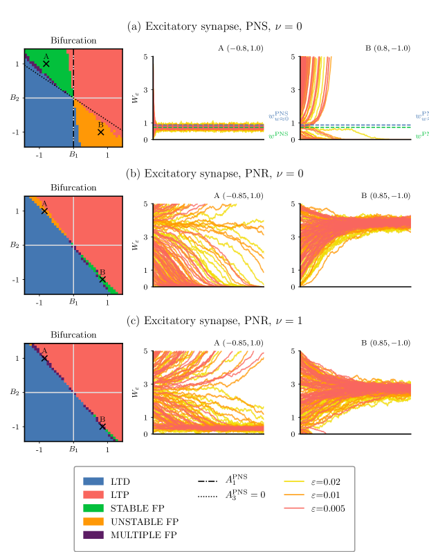
Figure 3. Different pairing schemes leads to diverse dynamics

Nearest neighbor symmetric STDP

For nearest neighbor symmetric STDP with $\displaystyle\beta(x){=}\nu{+}\beta x$, we derive in Appendix E.2.1, the associated dynamical system,

$$\frac{\mathop{}\mathopen{}\mathrm{d}w}{\mathop{}\mathopen{}\mathrm{d}t}(t)=f^{\text{\rm PNS}}(w)\stackrel{{\scriptstyle\text{\rm def}.}}{{=}}A^{\text{\rm PNS}}_{0}{+}A^{\text{\rm PNS}}_{1}w{+}A^{\text{\rm PNS}}_{2}h^{\text{\rm PNS}}(w),$$

with,

$$\displaystyle A^{\text{\rm PNS}}_{0} \displaystyle\stackrel{{\scriptstyle\text{\rm def}.}}{{=}}\frac{\nu\lambda}{\lambda{+}\gamma_{1}}B_{1}{+}\frac{\nu\lambda}{\nu{+}\gamma_{2}}B_{2},$$

$$\displaystyle A^{\text{\rm PNS}}_{1} \displaystyle\stackrel{{\scriptstyle\text{\rm def}.}}{{=}}\lambda\beta\frac{1{+}\lambda}{1{+}\lambda{+}\gamma_{1}}B_{1},\ A^{\text{\rm PNS}}_{2}{=}\lambda B_{2},$$

and

$$h^{\text{\rm PNS}}(w)\stackrel{{\scriptstyle\text{\rm def}.}}{{=}}\gamma_{2}\int_{\mathbb{R}_{+}}e^{-\gamma_{2}\tau}\left(1-\exp\left(\rule{0.0pt}{11.38109pt}{-}\nu\tau\right.\right.\\ \left.\left.{-}\lambda\int_{0}^{\tau}\left(1{-}\exp\left(-\beta w\left(1{-}e^{s-\tau}\right)\right)\right)\mathop{}\mathopen{}\mathrm{d}s\right.\right.\\ \left.\left.\rule{0.0pt}{11.38109pt}{-}\lambda\int_{-\infty}^{0}\left(1{-}\exp\left(-\beta w\left(1{-}e^{-\tau}\right)e^{s}\right)\right)\mathop{}\mathopen{}\mathrm{d}s\right)\right)\mathop{}\mathopen{}\mathrm{d}\tau-\frac{\nu}{\nu{+}\gamma_{2}}.$$

The asymptotic behavior of $\displaystyle(w(t))$ can be analyzed rigorously in this case, details in Appendix E.2.2.

If $\displaystyle\nu{=}0$, let

$$A^{\text{\rm PNS}}_{3}\stackrel{{\scriptstyle\text{\rm def}.}}{{=}}{f^{\text{\rm PNS}}}^{\prime}(0){=}\lambda\beta\left(\frac{1+\lambda}{1+\lambda+\gamma_{1}}B_{1}{+}\frac{\lambda}{\gamma_{2}}B_{2}\right)$$

• If $\displaystyle A^{\text{\rm PNS}}_{1}{<}0$ and $\displaystyle A^{\text{\rm PNS}}_{3}{<}0$, $\displaystyle(w(t))$ converges to $\displaystyle 0$ in finite time (blue).

• If $\displaystyle A^{\text{\rm PNS}}_{1}{>}0$ and $\displaystyle A^{\text{\rm PNS}}_{3}{>}0$, The system diverges to infinity when both parameters are positive (red).

• If $\displaystyle A^{\text{\rm PNS}}_{1}{<}0$ and $\displaystyle A^{\text{\rm PNS}}_{3}{>}0$, a stable fixed point $\displaystyle w^{\text{\rm PNS}}$ exists (green), see example $\displaystyle A$ $\displaystyle(B_{1},B_{2}){=}(-0.8,1)$.

• If $\displaystyle A^{\text{\rm PNS}}_{1}{>}0$ and $\displaystyle A^{\text{\rm PNS}}_{3}{<}0$, an unstable fixed point $\displaystyle w^{\text{\rm PNS}}$ exists (orange), example B.

In Appendix E.2.2, we prove the existence of the fixed point $\displaystyle w^{\text{\rm PNS}}$ and provided a numerical estimation in Figure 3(a). We compute an approximation of $\displaystyle w^{\text{\rm PNS}}$ when $\displaystyle w{\approx}0$ in E.2.2 is given, Figure 3(a) shows a comparison with numerical experiments.

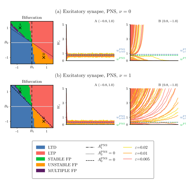
Figure 7. Nearest neighbor symetric pair-based STDP for an excitatory synapse

The picture is similar for the case $\displaystyle\nu{>}0$, with slightly different conditions (Appendix E.2.2 and Figure 7).

Discussion. Nearest neighbor symmetric STDP has significant differences with the all-to-all scheme. First, a positive stable (or unstable) fixed point may exist in the absence of external noise. The condition on $\displaystyle A^{\text{\rm PNS}}_{1}$ is a condition on $\displaystyle B_{1}$ only. If $\displaystyle B_{1}{<}0$ the system either converges to $\displaystyle 0$ or to a positive fixed point, and similarly when $\displaystyle B_{1}{>}0$. The all-to-all case does not exhibit such a simple behavior, because $\displaystyle A^{\text{\rm PA}}_{0}$ and $\displaystyle A^{\text{\rm PA}}_{1}$ both depend on $\displaystyle B_{1}$ and $\displaystyle B_{2}$.

Nearest neighbor symmetric reduced STDP

A theoretical study of $\displaystyle(w(t))$ solution of (3) with $\displaystyle\beta(x){=}\nu{+}\beta x$ is possible, but more involved than for PA and PNS. Some indications are given in the Appendix E.3. Computer simulations were done using this scheme and the results are illustrated in Figure 3(b) and (c). Surprisingly, we observe two different dynamics depending on the values of $\displaystyle\nu$.

For $\displaystyle\nu{=}0$, there exists a (narrow) range of parameters in the Hebbian region (bottom right) where a stable fixed point occurs, see example (B) in Figure 3(b). Symmetrically, an unstable fixed point seems to exist in the anti-Hebbian region (top left) and example (A).

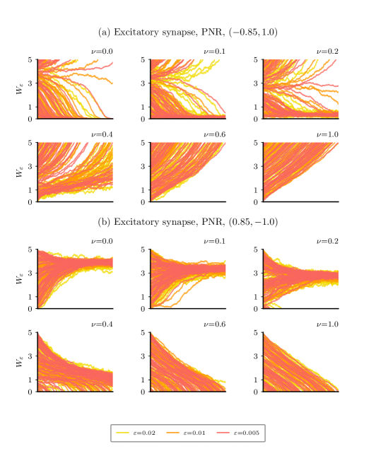
Figure 5. Influence of $\displaystyle\nu$ on dynamics with the pair-based nearest-neighbor reduced symmetric scheme

For $\displaystyle\nu{>}0$, a second fixed point appears leading to more complex behaviors characterized by the presence of a stable and an unstable fixed point at the same time Figure 3(c). If the stable fixed point is lower than the unstable one, see example (A) and (top left) in Figure 3(c), the synaptic weight either converges to a non null value or diverges to infinity. For Hebbian parameters (bottom right), the situation is reversed, see example (B) in Figure 3(c). The spectrum of values with this complex behavior narrows when $\displaystyle\nu$ is increasing. In particular, for large values of $\displaystyle\nu$, only a perfect balance in the parameters may lead to other behaviors than whole depression or potentiation. We have studied this influence of $\displaystyle\nu$, on the dynamics, for $\displaystyle B_{1}$ and $\displaystyle B_{2}$ constant in Figure 5.

Discussion. There are several differences of interest with the two other STDP pair-based rules for an excitatory synapse. First, for all-to-all and nearest neighbor symmetric pairings at an excitatory synapse, the stable fixed point only appears for anti-Hebbian parameters, $\displaystyle B_{1}{<}0$, whereas an unstable one exists for Hebbian STDP, $\displaystyle B_{1}{>}0$. With nearest neighbor symmetric reduced STDP, we have numerically shown that a more complex behavior with several fixed points may occur.

Second, the nearest neighbor symmetric reduced STDP needs an almost exact balance of the parameters to enable convergence of the system toward a fixed point.

Table 3 gathers up all results for an excitatory synapse.

3.3. All-to-all STDP with an inhibitory synapse

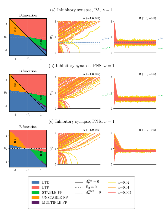
Figure 4. Pair-based STDP for an inhibitory synapse

We now study the dynamics (3) of the synaptic weight for an inhibitory synapse, i.e. when $\displaystyle\beta(x){=}(\nu{-}\beta x)^{+}$.

Computations of $\displaystyle f^{\text{\rm PA}}$ are detailed in Appendix E.4. We restrict our study to two cases.

For small $\displaystyle w$,

$$\displaystyle\frac{\mathop{}\mathopen{}\mathrm{d}w}{\mathop{}\mathopen{}\mathrm{d}t}(t) \displaystyle=f^{\text{\rm PA}}(w)=A^{\text{\rm PA}}_{0}{-}A^{\text{\rm PA}}_{1}w{+}o(w)$$

$$\displaystyle={-}A^{\text{\rm PA}}_{1}\left(w{+}w^{\text{\rm PA}}\right){+}o(w).$$

with $\displaystyle A^{\text{\rm PA}}_{0/1}$ defined before.

When $\displaystyle w\geq\nu/\beta$, we have

$$\frac{\mathop{}\mathopen{}\mathrm{d}w}{\mathop{}\mathopen{}\mathrm{d}t}(t)=\frac{A^{\text{\rm PAI}}}{w(t)^{\lambda+\gamma_{1}}}\left(1{+}\eta^{\text{\rm PAI}}\left[\frac{w(t)}{w^{\text{\rm PAI}}}\right]^{\gamma_{1}}\right)$$

with

$$A^{\text{\rm PAI}}\stackrel{{\scriptstyle\text{\rm def}.}}{{=}}\left[\frac{\nu}{\beta}\right]^{\lambda+\gamma_{1}}\frac{c(\lambda)B_{1}\nu}{\left(\lambda+\gamma_{1}\right)\left(\lambda{+}\gamma_{1}{+}1\right)},$$

$$w^{\text{\rm PAI}}\stackrel{{\scriptstyle\text{\rm def}.}}{{=}}\frac{\beta}{\nu}\left(\left|\frac{B_{2}}{B_{1}}\right|\frac{\left(\lambda{+}\gamma_{1}\right)\left(\lambda+\gamma_{1}{+}1\right)}{\gamma_{2}\left(\lambda+1\right)}\right)^{1/\gamma_{1}},$$

$$\eta^{\text{\rm PAI}}\stackrel{{\scriptstyle\text{\rm def}.}}{{=}}\left|\frac{B_{2}}{B_{1}}\right|\frac{B_{1}}{B_{2}}.$$

For stability properties, the two relevant parameters are $\displaystyle A^{\text{\rm PA}}_{0}$ and $\displaystyle B_{2}$.

• For $\displaystyle B_{2}{>}0$ and $\displaystyle A^{\text{\rm PA}}_{0}{>}0$, the synaptic weight diverges to infinity (in red),

• For $\displaystyle B_{2}{<}0$ and $\displaystyle A^{\text{\rm PA}}_{0}{<}0$, it converges to $\displaystyle 0$ in finite time (in blue).

• For $\displaystyle B_{2}{>}0$ and $\displaystyle A^{\text{\rm PA}}_{0}{<}0$, there is an unstable fixed point (orange, example A).

• For $\displaystyle B_{2}{<}0$ and $\displaystyle A^{\text{\rm PA}}_{0}{>}0$, the system exhibits a stable equilibrium (green, example B).

We note here an inversion with the properties observed for the excitatory synapse, where only anti-Hebbian STDP led to a stable fixed point, compared to the inhibitory case where only Hebbian STDP elicits this type of behavior.

Moreover, $\displaystyle A^{\text{\rm PA}}_{0}{=}0$ corresponds to the line $\displaystyle w^{\text{\rm PA}}{=}0$, suggesting that an important parameter for the classification of behavior is the range of parameters where $\displaystyle w^{\text{\rm PA}}{=}0$ for the excitatory case.

This analysis is completed with the other schemes in Figure 4(b) for PNS and Figure 4(c) for PNR. The dynamics are similar to the all-to-all case for this range of parameters, only the values of the fixed points seems to change (compare B for the three cases). For the nearest neighbor symmetric STDP, we also plotted the line $\displaystyle w^{\text{\rm PNS}}{=}0$, as it could be related to the change of dynamics following the analysis of the all-to-all case.

All these behaviors are gathered in Table 4. It is striking that the pairing scheme does not seem to have a decisive impact on the dynamics for an inhibitory synapse, contrarily to the case of an excitatory synapse. This may be due to the fact that for the inhibitory case, we need to have a constant external input in order to have spikes. We note here that, for the sake of simplicity, we only tested cases where $\displaystyle\nu{=}1$.

4. Conclusion

We have developed a simple and rigorous analysis of synaptic weight dynamics via a slow-fast approximation and numerical simulations. For an excitatory synapse, anti-Hebbian STDP can lead to a stable fixed point, with some slight variations depending on the pairing scheme used. In particular, for all-to-all STDP rules, a fixed point exists only for positive external rate $\displaystyle\nu$, whereas for nearest symmetric reduced scheme, at least two fixed points exists for balanced STDP rules. Moreover, for an inhibitory synapse, numerical arguments showed that all schemes were similar, with the existence of a stable fixed point for Hebbian STDP.

In a learning paradigm, a subset of correlated neurons are able to repeatedly trigger an action potential of the postsynaptic neuron, even in the presence of noise. It is not a surprise then if this regime of activity led to the most interesting behaviors for the synaptic weight dynamics of our study. Indeed, when the influence of a single neuron (or by extension a group of correlated neurons) is not negligible compared to the rest of inputs (when $\displaystyle\lambda w{>}\nu$), the asymptotic behavior of the synaptic weight highly depends on the polarity of the STDP curve and the pairing scheme.

On the contrary, when the impact of the presynaptic neuron spikes is lost in the external noise (consistent with a large number of external uncorrelated inputs, $\displaystyle\lambda w{<}\nu$), pairing schemes do not influence the type of dynamics observed. Indeed, the influence of ‘direct’ and ‘repetitive’ pairings is lost in the large noise limit: in mean-field models, the synaptic weight dynamics is essentially driven by the mean synaptic weight, see [1].

This work highlights the fact that the choice of spikes to take into account in STDP is an essential part of the modeling process. In particular, this conclusion should apply to more complex pairing schemes such as triplets rules [27, 1] or more complex calcium-based rules.

If this article focuses on a single synapse dynamics, its conclusions can be used to explain some of the results from the literature on the influence of STDP in recurrent networks [5, 15, 40]. [22] studies short-term plasticity in a large network and [23] the noise-enhanced coupling of two excitatory neurons subject to STDP, which can be extended to the formation of multiclusters in adaptive networks [2]. It would be challenging to extend our results to large stochastic networks with plastic synapses where theoretical studies are scarce. Multi-dimensional auto-exciting/inhibiting processes are an important tool in this context. In particular Hawkes processes, see [28, 9]. This is a promising approach toward a better understanding of learning in adaptive neural systems.

Appendix A Computer methods

For each set of parameters, we have run several simulations, with different initial weight values uniformly taken in $\displaystyle[0,w_{\text{\rm max}}]$. We have tested the dynamics of the synaptic weight for the different pairing schemes defined before for a wide range of parameters. Simulations have been done using Python 3.X for the simple network of a pre-synaptic and a post-synaptic neuron. We used a discrete Euler scheme for the dynamics of the membrane potential $\displaystyle X$ and the plasticity variables $\displaystyle Z_{1}$ and $\displaystyle Z_{2}$. Whenever the synaptic weight was either $\displaystyle 0$ or a maximal value $\displaystyle w_{\text{\rm max}}$ the dynamics was stopped and the synaptic weight state recorded.

We also plot the temporal dynamics for specific values of $\displaystyle B_{1}$ and $\displaystyle B_{2}$, typically used $\displaystyle P{=}50$ simulations for each scaling $\displaystyle\varepsilon$.

Appendix B Pair-based STDP with different pairing schemes

All-to-all Model

The all-to-all pair-based model supposes that all pairs of spikes are taken into account in the synaptic plasticity rule. The synaptic weight is updated at each post-synaptic spike occurring at time $\displaystyle t_{\rm post}$, by taking into account all pre-synaptic spikes before time $\displaystyle t_{\rm post}$:

$$\Delta W(t_{\rm post})=B_{1}\sum_{t_{{\rm pre},n}{<}t_{\rm post}}e^{-\gamma_{1}(t_{\rm post}{-}t_{{\rm pre},n})}=Z_{1}^{\rm PA}(t_{\rm post})$$

and,

$$\Delta W(t_{\rm pre})=B_{2}\sum_{t_{{\rm post},n}{<}t_{\rm pre}}e^{-\gamma_{2}(t_{\rm pre}{-}t_{{\rm post},n})}=Z_{2}^{\rm PA}(t_{\rm pre})$$

The processes $\displaystyle(Z_{i}^{\rm PA}(t))$, $\displaystyle i{=}1$, $\displaystyle 2$ can be expressed as solutions of the stochastic differential equations,

(5) $$\begin{cases}\mathop{}\mathopen{}\mathrm{d}Z_{1}^{\rm PA}(t)\displaystyle={-}\gamma_{1}Z_{1}^{\rm PA}(t)\mathop{}\mathopen{}\mathrm{d}t+B_{1}\mathcal{N}_{\lambda}(\mathop{}\mathopen{}\mathrm{d}t),\\ \mathop{}\mathopen{}\mathrm{d}Z_{2}^{\rm PA}(t)\displaystyle={-}\gamma_{2}Z_{2}^{\rm PA}(t)\mathop{}\mathopen{}\mathrm{d}t+B_{2}\mathcal{N}_{\beta,X}(\mathop{}\mathopen{}\mathrm{d}t),\end{cases}$$

they are two shot-noise processes, see [14, 30].

The synaptic weight updates correspond to the evaluation of $\displaystyle(Z_{1}^{\rm PA}(t))$ at jumps of the point process $\displaystyle{\cal N}_{\beta,X}$ for post-synaptic activity, and similarly for $\displaystyle(Z_{2}^{\rm PA}(t))$ with $\displaystyle{\cal N}_{\lambda}$,

$$\displaystyle\mathop{}\mathopen{}\mathrm{d}W^{\rm PA}(t) \displaystyle=\sum_{t_{{\rm pre},n}}Z_{2}^{\rm PA}(t_{{\rm pre},n}-)\delta_{t_{{\rm pre},n}}$$

$$\displaystyle\hskip 28.45274pt+\sum_{t_{\rm post},n}Z_{1}^{\rm PA}(t_{{\rm post},n}-)\delta_{t_{\rm post},n},$$

or, equivalently,

$$\mathop{}\mathopen{}\mathrm{d}W^{\rm PA}(t)=Z_{2}^{\rm PA}(t-){\cal N}_{\lambda}(\mathop{}\mathopen{}\mathrm{d}t)+Z_{1}^{\rm PA}(t-){\cal N}_{\beta,X}(\mathop{}\mathopen{}\mathrm{d}t).$$

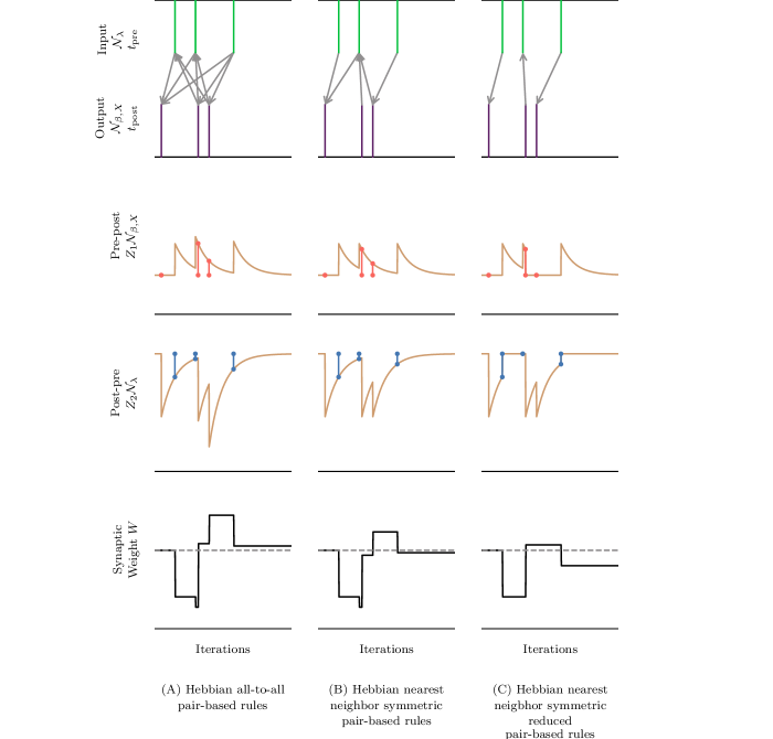
Figure 6. Markovian formulation of pair-based models

The notation $\displaystyle U(t{-})$ is for the left limit of the function $\displaystyle(U(t))$ at $\displaystyle t$. A simple example of the dynamics of the all-to-all pair-based model is depicted in Figure 6 (A) with interacting pairs of spikes.

Nearest-neighbor symmetric model

In the nearest neighbor symmetric model, whenever one neuron spikes, the synaptic weight is updated by only taking into account the last spike of the other neuron, as can be seen in Figure 1. If the pre-synaptic neuron fires at time $\displaystyle t_{\rm pre}$, the contribution to the plasticity kernel is $\displaystyle\Phi(t_{\rm pre}{-}t_{\rm post})$ , where $\displaystyle t_{\rm post}$ is the last post-synaptic spike before $\displaystyle t_{\rm pre}$ and similarly for post-synaptic spikes.

The nearest neighbor symmetric rule leads to,

(6) $$\begin{cases}\mathop{}\mathopen{}\mathrm{d}Z_{1}^{\rm PNS}(t)\displaystyle&={-}\gamma_{1}Z_{1}^{\rm PNS}(t)\mathop{}\mathopen{}\mathrm{d}t\\ &+(B_{1}-Z_{1}^{\rm PNS}(t-))\mathcal{N}_{\lambda}(\mathop{}\mathopen{}\mathrm{d}t),\\ \mathop{}\mathopen{}\mathrm{d}Z_{2}^{\rm PNS}(t)\displaystyle&={-}\gamma_{2}Z_{2}^{\rm PNS}(t)\mathop{}\mathopen{}\mathrm{d}t\\ &+(B_{2}-Z_{2}^{\rm PNS}(t-)))\mathcal{N}_{\beta,X}(\mathop{}\mathopen{}\mathrm{d}t).\end{cases}$$

At each pre-synaptic spike, $\displaystyle(Z_{1}^{\rm PNS}(t))$, resp. $\displaystyle(Z_{2}^{\rm PNS}(t))$, is reset to $\displaystyle B_{1}$, resp. $\displaystyle B_{2}$. See Figure 6 (B).

Nearest-neighbor symmetric reduced model

Finally, for the nearest neighbor symmetric reduced scheme, only consecutive pairs of spikes are used to update the synaptic weight. The synaptic weight is updated at pre-synaptic spike time $\displaystyle t_{\rm pre}$ only if there are no pre-synaptic spikes since the last post-synaptic spike. And similarly for post-synaptic spike times. See Figure 1 (bottom right).

This rule leads to $\displaystyle(Z_{i}^{\rm PNR}(t))$, $\displaystyle i{=}1$, $\displaystyle 2$, solutions of

(7) $$\begin{cases}\mathop{}\mathopen{}\mathrm{d}Z_{1}^{\rm PNR}(t)\displaystyle&={-}\gamma_{1}Z_{1}^{\rm PNR}(t)\mathop{}\mathopen{}\mathrm{d}t\\ &+(B_{1}-Z_{1}^{\rm PNR}(t-))\mathcal{N}_{\lambda}(\mathop{}\mathopen{}\mathrm{d}t)\\ &-Z_{1}^{\rm PNR}(t-))\mathcal{N}_{\beta,X}(\mathop{}\mathopen{}\mathrm{d}t),\\ \mathop{}\mathopen{}\mathrm{d}Z_{2}^{\rm PNR}(t)\displaystyle&={-}\gamma_{2}Z_{2}^{\rm PNR}(t)\mathop{}\mathopen{}\mathrm{d}t\\ &+(B_{2}-Z_{2}^{\rm PNR}(t-)))\mathcal{N}_{\beta,X}(\mathop{}\mathopen{}\mathrm{d}t)\\ &-Z_{2}^{\rm PNR}(t-)\mathcal{N}_{\lambda}(\mathop{}\mathopen{}\mathrm{d}t).\end{cases}$$

See Figure 6 (C).

Appendix C Slow-fast approximations, averaging principles

We have the scaled system, for $\displaystyle\varepsilon{>}0$,

(8) $$\begin{cases}\mathop{}\mathopen{}\mathrm{d}X_{\varepsilon}(t)&={-}1/\varepsilon X_{\varepsilon}(t)\mathop{}\mathopen{}\mathrm{d}t+W_{\varepsilon}(t{-})\mathcal{N}_{\lambda/\varepsilon}(\mathop{}\mathopen{}\mathrm{d}t),\\ \mathop{}\mathopen{}\mathrm{d}Z_{1,\varepsilon}(t)&={-}\gamma_{1}Z_{1,\varepsilon}(t)\mathop{}\mathopen{}\mathrm{d}t/\varepsilon\\ &\hskip 5.69054pt+(B_{1}-K_{1,1}Z_{1,\varepsilon}(t{-}))\mathcal{N}_{\lambda/\varepsilon}(\mathop{}\mathopen{}\mathrm{d}t)\\ &\hskip 5.69054pt-K_{1,2}Z_{1,\varepsilon}(t{-})\mathcal{N}_{\beta/\varepsilon,X_{\varepsilon}}(\mathop{}\mathopen{}\mathrm{d}t),\\ \mathop{}\mathopen{}\mathrm{d}Z_{2,\varepsilon}(t)&={-}\gamma_{2}Z_{2,\varepsilon}(t)\mathop{}\mathopen{}\mathrm{d}t/\varepsilon\\ &\hskip 5.69054pt+(B_{2}{-}K_{2,2}Z_{2,\varepsilon}(t{-}))\mathcal{N}_{\beta/\varepsilon,X_{\varepsilon}}(\mathop{}\mathopen{}\mathrm{d}t)\\ &\hskip 5.69054pt-K_{2,1}Z_{2,\varepsilon}(t{-})\mathcal{N}_{\lambda/\varepsilon}(\mathop{}\mathopen{}\mathrm{d}t),\\ \mathop{}\mathopen{}\mathrm{d}W_{\varepsilon}(t)&=Z_{1,\varepsilon}(t{-})\varepsilon\mathcal{N}_{\beta/\varepsilon,X_{\varepsilon}}(\mathop{}\mathopen{}\mathrm{d}t)\\ &\hskip 5.69054pt+Z_{2,\varepsilon}(t{-})\varepsilon\mathcal{N}_{\lambda/\varepsilon}(\mathop{}\mathopen{}\mathrm{d}t)\end{cases}$$

where $\displaystyle\gamma_{1},\gamma_{2}{>}0$, $\displaystyle B_{1},B_{2}{\in}\mathbb{R}$, $\displaystyle{\mathbf{K}}{=}(K_{ij},i,j{\in}\{1,2\}){\in}\{0,1\}^{4}$.

Approximations of $\displaystyle(W_{\varepsilon}(t))$ solution of (1) when $\displaystyle\varepsilon$ is small are discussed and investigated with ad-hoc methods. The corresponding scaling results, known as separation of timescales, are routinely used in approximations in mathematical models of computational neuroscience, for example [20].

We first need to define the processes $\displaystyle(X^{w}(t),Z_{1}^{w}(t),Z_{2}^{w}(t))$ which follow the fast processes dynamics with a constant synaptic weight $\displaystyle w$ and prove that a unique invariant distribution exists for the associated dynamics. This is the purpose of Proposition 1.

Proposition 1 (Equilibrium of Fast Processes).

For $\displaystyle{\mathbf{K}}{=}(K_{ij},i,j{\in}\{1,2\}){\in}\{0,1\}^{4}$, $\displaystyle\gamma_{1},\gamma_{2}{>}0$, $\displaystyle B_{1},B_{2}{\in}\mathbb{R}$, and each $\displaystyle w{\geq}0$, the Markov process $\displaystyle(X^{w}(t),Z_{1}^{w}(t),Z_{2}^{w}(t))$ solution of (2) has a unique stationary distribution $\displaystyle\Pi_{w}^{\mathbf{K}}$ on $\displaystyle\mathbb{R}_{+}{\times}\mathbb{R}^{2}$.

Proof.

See Proposition 25 of [29]. ∎

Theorem 1 (Averaging Principle).

There exists $\displaystyle S_{0}{\in}(0,{+}\infty]$ such that, when $\displaystyle\varepsilon$ goes to $\displaystyle 0$, the process $\displaystyle(W_{\varepsilon}(t),t{<}S_{0})$ is converging in distribution to $\displaystyle(w(t),t{<}S_{0})$, solution of the equation

$$\frac{\mathop{}\mathopen{}\mathrm{d}w}{\mathop{}\mathopen{}\mathrm{d}t}(t)=\mathbb{E}_{\Pi^{\mathbf{K}}_{w(t)}}\left[\lambda Z_{2}{+}\beta(X)Z_{1}\right],$$

where $\displaystyle\Pi^{K}_{w}$ is defined in Proposition 1.

Proof.

See [31] and [29]. ∎

Appendix D Comparison to classical computational models

In this section, we compare averaging principles for STDP rules leading to Relation (3) with the results of [20] in the all-to-all pair-based scheme.

The asymptotic behavior of the synaptic weight dynamics, Relation (4) of [20], is a consequence of a similar slow-fast argument,

(9) $$\frac{\mathop{}\mathopen{}\mathrm{d}\widetilde{w}}{\mathop{}\mathopen{}\mathrm{d}t}(t)=\int_{-\infty}^{+\infty}\widetilde{\Phi}(s)\widetilde{\mu}(s,t)\mathop{}\mathopen{}\mathrm{d}s,$$

where,

• $\displaystyle\widetilde{\Phi}(s)$ represents the STDP curve;

• $\displaystyle\widetilde{\mu}(s,t){=}\overline{{<}S^{1}(t{+}s)S^{2}(t){>}}$, the correlation between the spike trains.

The quantity $\displaystyle\overline{\left<{\cdots}\right>}$ is defined in terms of temporal and ensemble averages, $\displaystyle{<}{\cdots}{>}$ is the ensemble average and $\displaystyle\overline{\cdots}$ the temporal average over the spike trains.

In our setting, Theorem 1 gives the following equation,

$$\frac{\mathop{}\mathopen{}\mathrm{d}w}{\mathop{}\mathopen{}\mathrm{d}t}(t)=\mathbb{E}_{\Pi^{\text{\rm PA}}_{w(t)}}\left[\lambda Z_{2}{+}\beta(X)Z_{1}\right],$$

with

$$\Phi(t)\stackrel{{\scriptstyle\text{\rm def}.}}{{=}}B_{1}\exp(-\gamma_{1}t)\mathbbm{1}_{\left\{t>0\right\}}+B_{2}\exp(\gamma_{2}t)\mathbbm{1}_{\left\{t<0\right\}}.$$

We have, using simple calculus,

$$\lambda\mathbb{E}_{\Pi^{\text{\rm PA}}_{w(t)}}\left[Z_{2}\right]=\int_{-\infty}^{0}B_{2}\exp(\gamma_{2}\tau)\lambda\mathbb{E}_{\Pi^{\text{\rm PA}}_{w(t)}}\left[\beta(x)\right]\mathop{}\mathopen{}\mathrm{d}\tau$$

We denote by $\displaystyle\Pi^{\text{\rm PA}}_{2{\mapsto}1,t}(\tau)$ the probability of having a post-pre pairing with delay $\displaystyle\tau$ at time $\displaystyle t$. For the post-pre pairing, we can consider that $\displaystyle\Pi^{\text{\rm PA}}_{2{\mapsto}1,t}(\tau)$ does not depend on $\displaystyle\tau$ and that it is just equal to the product of both rates, i.e there is no causality, and

$$\Pi^{\text{\rm PA}}_{2{\mapsto}1,t}(\tau)=\lambda\mathbb{E}_{\Pi^{\text{\rm PA}}_{w(t)}}\left[\beta(x)\right].$$

We easily conclude that,

$$\lambda\mathbb{E}_{\Pi^{\text{\rm PA}}_{w(t)}}\left[Z_{2}\right]=\int_{-\infty}^{0}\Phi(\tau)\Pi^{\text{\rm PA}}_{2{\mapsto}1,t}(\tau)\mathop{}\mathopen{}\mathrm{d}\tau,$$

with $\displaystyle\Pi^{\text{\rm PA}}_{2{\mapsto}1,t}(\tau)\approx\overline{{<}S^{1}(t{+}\tau)S^{2}(t){>}}$.

Similarly, we have

$$\mathbb{E}_{\Pi^{\text{\rm PA}}_{w(t)}}\left[\beta(X)Z_{1}\right]=\mathbb{E}_{\Pi^{\text{\rm PA}}_{w(t)}}\left[\sum_{t_{\text{\rm pre}}{<}t_{\text{\rm post}}}B_{1}\exp(-\gamma_{1}(t_{\text{\rm post}}-t_{\text{\rm pre}}))\beta(X)\right]$$

We denote by $\displaystyle\Pi^{\text{\rm PA}}_{1{\mapsto}2,t}(\tau)$ the probability of having a pre-post pairing with delay $\displaystyle\tau$ at time $\displaystyle t$. For the pre-post pairing, this quantity depends on $\displaystyle\tau$ because spikes of the pre-synaptic neuron influence the spiking of the post-synaptic one, so we have, by using the fact that $\displaystyle\Pi^{\text{\rm PA}}$ is the invariant distribution,

$$\mathbb{E}_{\Pi^{\text{\rm PA}}_{w(t)}}\left[\sum_{t_{\text{\rm pre}}{<}t_{\text{\rm post}}}B_{1}\exp(-\gamma_{1}(t_{\text{\rm post}}-t_{\text{\rm pre}}))\beta(X)\right]=\\ \int_{0}^{+\infty}B_{1}\exp(-\gamma_{1}\tau)\Pi^{\text{\rm PA}}_{1{\mapsto}2,t}(\tau)\mathop{}\mathopen{}\mathrm{d}\tau.$$

See SM2 of [31], hence

$$\mathbb{E}_{\Pi^{\text{\rm PA}}_{w(t)}}\left[\beta(X)Z_{1}\right]=\int_{0}^{+\infty}\Phi(\tau)\Pi^{\text{\rm PA}}_{1{\mapsto}2,t}(\tau)\mathop{}\mathopen{}\mathrm{d}\tau,$$

with $\displaystyle\Pi^{\text{\rm PA}}_{1{\mapsto}2,t}(\tau)\approx\overline{{<}S^{1}(t)S^{2}(t{+}\tau){>}}$. This shows the equivalence between [20] and our result for the all-to-all pair-based STDP rules.

Appendix E Proofs

E.1. All-to-all STDP at an excitatory synapse

We prove that,

$$\mathbb{E}_{\Pi^{\textup{PA}}_{w(t)}}\left[\lambda Z_{2}{+}\beta(X)Z_{1}\right]=A^{\text{\rm PA}}_{0}{+}A^{\text{\rm PA}}_{1}w=A^{\text{\rm PA}}_{1}\left(w{-}w^{\text{\rm PA}}\right).$$

where,

$$A^{\text{\rm PA}}_{0}=\nu\lambda\left(\frac{B_{1}}{\gamma_{1}}{+}\frac{B_{2}}{\gamma_{2}}\right),\,A^{\text{\rm PA}}_{1}=\beta\lambda^{2}\left(\frac{B_{1}}{\gamma_{1}}{+}\frac{B_{2}}{\gamma_{2}}{+}\frac{B_{1}}{\lambda(1{+}\gamma_{1})}\right)$$

Proof.

First, it is easy to show that,

$$\mathbb{E}\left[Z^{\textup{PA},w}_{1}\right]=\lambda\frac{B_{1}}{\gamma_{1}},\text{ and }\mathbb{E}\left[Z^{\textup{PA},w}_{2}\right]=\nu\frac{B_{2}}{\gamma_{2}}{+}\beta\lambda\frac{B_{2}}{\gamma_{2}}w$$

Moreover, denoting $\displaystyle(Y^{w}(t)){=}(X^{w}(t)Z^{\textup{PA},w}_{1}(t))$, we get

$$\mathop{}\mathopen{}\mathrm{d}Y^{w}(t)={-}(1{+}\gamma_{1})Y^{w}(t)\mathop{}\mathopen{}\mathrm{d}t+\left(\rule{0.0pt}{11.38109pt}wZ^{\textup{PA},w}_{1}(t{-}){+}B_{1}X^{w}(t{-})+wB_{1}\right){\cal N}_{\lambda}(\mathop{}\mathopen{}\mathrm{d}t),$$

by integrating this ODE on $\displaystyle[0,t]$ and taking the expected value, we obtain

$$\mathbb{E}\left[X^{w}Z^{\textup{PA},w}_{1}\right]=\frac{\lambda w\mathbb{E}\left[Z^{\textup{PA},w}_{1}\right]{+}\lambda B_{1}\mathbb{E}\left[X^{w}\right]{+}\lambda wB_{1}}{1{+}\gamma_{1}}=\left(\frac{\lambda^{2}}{\gamma_{1}}{+}\frac{\lambda}{1{+}\gamma_{1}}\right)B_{1}w.$$

∎

E.2. Nearest neighbor symmetric STDP at an excitatory synapse

E.2.1. Estimation of $\displaystyle f^{\text{\rm PNS}}$

$$\mathbb{E}_{\Pi^{\textup{PNS}}_{w(t)}}\left[\lambda Z_{2}{+}\beta(X)Z_{1}\right]=A^{\text{\rm PNS}}_{0}{+}A^{\text{\rm PNS}}_{1}w{+}A^{\text{\rm PNS}}_{2}h^{\text{\rm PNS}}(w)$$

with,

$$A^{\text{\rm PNS}}_{0}{=}\frac{\nu\lambda}{\lambda{+}\gamma_{1}}B_{1}{+}\frac{\nu\lambda}{\nu{+}\gamma_{2}}B_{2},\,A^{\text{\rm PNS}}_{1}{=}\lambda\beta\frac{1{+}\lambda}{1{+}\lambda{+}\gamma_{1}}B_{1},\ A^{\text{\rm PNS}}_{2}{=}\lambda B_{2},$$

and,

$$h^{\text{\rm PNS}}(w)=\gamma_{2}\int_{\mathbb{R}_{+}}e^{-\gamma_{2}\tau}\left(1-\exp\left(\rule{0.0pt}{11.38109pt}{-}\nu\tau{-}\lambda\int_{0}^{\tau}\left(1{-}\exp\left({-}\beta w\left(1{-}e^{s-\tau}\right)\right)\right)\mathop{}\mathopen{}\mathrm{d}s\right.\right.\\ \displaystyle\hskip 85.35826pt\left.\left.\rule{0.0pt}{11.38109pt}{-}\lambda\int_{-\infty}^{0}\left(1{-}\exp\left({-}\beta w\left(1{-}e^{-\tau}\right)e^{s}\right)\right)\mathop{}\mathopen{}\mathrm{d}s\right)\right)\mathop{}\mathopen{}\mathrm{d}\tau{-}\frac{\nu}{\nu{+}\gamma_{2}}.$$

Proof.

For $\displaystyle w{\geq}0$, we have,

$$f^{\text{\rm PNS}}(w)=\nu B_{2}\int_{\mathbb{R}_{+}}\lambda e^{-(\lambda+\gamma_{2})\tau}\mathop{}\mathopen{}\mathrm{d}\tau{+}\lambda\beta wB_{1}\int_{\mathbb{R}_{+}}(1{+}\lambda)e^{-(1{+}\lambda{+}\gamma_{1})\tau}\mathop{}\mathopen{}\mathrm{d}\tau\\ {-}\lambda\gamma_{2}\int_{\mathbb{R}_{+}}\exp(-\gamma_{2}\tau)\left(1-\exp\left(\rule{0.0pt}{11.38109pt}{-}\nu\tau{-}\lambda\int_{0}^{\tau}\left(1{-}\exp\left(-\beta w\left(1{-}e^{s-\tau}\right)\right)\right)\mathop{}\mathopen{}\mathrm{d}s\right.\right.\\ \displaystyle\hskip 28.45274pt\left.\left.\rule{0.0pt}{11.38109pt}{-}\lambda\int_{-\infty}^{0}\left(1{-}\exp\left(-\beta w\left(1{-}e^{-\tau}\right)e^{s}\right)\right)\mathop{}\mathopen{}\mathrm{d}s\right)\right)\mathop{}\mathopen{}\mathrm{d}\tau.$$

Stochastic calculus gives, for $\displaystyle\xi{\geq}0$,

$${-}\ln\mathbb{E}\left[e^{{-}\xi{\cal N}_{\beta,X^{w}_{\infty}}((0,a))}\right]{=}\nu a\left(\!1{-}e^{-\xi}\!\right){+}\lambda\!\!\int_{0}^{a}\left(1{-}\exp\left(-\beta w\left(1{-}e^{{-}\xi}\right)\!\!\left(1{-}e^{s-a}\right)\right)\right)\!\mathop{}\mathopen{}\mathrm{d}s\\ {+}\lambda\int_{-\infty}^{0}\left(1{-}\exp\left(-\beta w\left(1{-}e^{-\xi}\right)\left(1{-}e^{-a}\right)e^{s}\right)\right)\mathop{}\mathopen{}\mathrm{d}s.$$

By letting $\displaystyle\xi$ go to infinity, we have obtained the desired expression. The proposition is proved.

∎

E.2.2. Dynamics of $\displaystyle w$

We start with some calculations for $\displaystyle h^{\text{\rm PNS}}$ of Section 3.2.

Lemma 1.

$\displaystyle h^{\text{\rm PNS}}$ is a convex function, and,

$$h^{\text{\rm PNS}}(0)=0,\,h^{\text{\rm PNS}}({+}\infty)=1{-}\frac{\nu}{\nu{+}\gamma_{2}},\,{h^{\text{\rm PNS}}}^{\prime}(0)=\frac{\lambda\beta\gamma_{2}}{(\nu{+}\gamma_{2})^{2}}$$

Proof.

We compute,

$${h^{\text{\rm PNS}}}^{\prime}(w)=\lambda\beta\gamma_{2}\int_{\mathbb{R}_{+}}e^{-(\nu+\gamma_{2})\tau}\left(\int_{0}^{\tau}\left(1{-}e^{s-\tau}\right)\exp\left(-\beta w\left(1{-}e^{s-\tau}\right)\right)\mathop{}\mathopen{}\mathrm{d}s\right.\\ \left.{+}\int_{-\infty}^{0}\left(1{-}e^{-\tau}\right)e^{s}\exp\left(-\beta w\left(1{-}e^{-\tau}\right)e^{s}\right)\mathop{}\mathopen{}\mathrm{d}s\right)\\ \exp\left(\rule{0.0pt}{11.38109pt}{-}\lambda\int_{0}^{\tau}\left(1{-}\exp\left(-\beta w\left(1{-}e^{s-\tau}\right)\right)\right)\mathop{}\mathopen{}\mathrm{d}s{-}\lambda\int_{-\infty}^{0}\left(1{-}\exp\left(-\beta w\left(1{-}e^{-\tau}\right)e^{s}\right)\right)\mathop{}\mathopen{}\mathrm{d}s\right)\mathop{}\mathopen{}\mathrm{d}\tau.$$

We have $\displaystyle h^{\prime}(w)$ is an increasing function in $\displaystyle w$, so $\displaystyle h(w)$ is convex. ∎

The system

$$\frac{\mathop{}\mathopen{}\mathrm{d}w}{\mathop{}\mathopen{}\mathrm{d}t}(t)=A^{\text{\rm PNS}}_{0}{+}A^{\text{\rm PNS}}_{1}w{+}A^{\text{\rm PNS}}_{2}h^{\text{\rm PNS}}(w)$$

has the following dynamics.

$\displaystyle\nu$	LTD	LTP	STABLE FP	UNSTABLE FP
$\displaystyle 0$	$\displaystyle A^{\text{\rm PNS}}_{3}{<}0$	$\displaystyle A^{\text{\rm PNS}}_{3}{>}0$	$\displaystyle A^{\text{\rm PNS}}_{3}{<}0$	$\displaystyle A^{\text{\rm PNS}}_{3}{>}0$
	$\displaystyle A^{\text{\rm PNS}}_{1}{<}0$	$\displaystyle A^{\text{\rm PNS}}_{1}{>}0$	$\displaystyle A^{\text{\rm PNS}}_{1}{>}0$	$\displaystyle A^{\text{\rm PNS}}_{1}{<}0$
$\displaystyle>0$	$\displaystyle A^{\text{\rm PNS}}_{0}{<}0$	$\displaystyle A^{\text{\rm PNS}}_{0}{>}0$	$\displaystyle A^{\text{\rm PNS}}_{0}{<}0$	$\displaystyle A^{\text{\rm PNS}}_{0}{>}0$
	$\displaystyle A^{\text{\rm PNS}}_{1}{<}0$	$\displaystyle A^{\text{\rm PNS}}_{1}{>}0$	$\displaystyle A^{\text{\rm PNS}}_{1}{>}0$	$\displaystyle A^{\text{\rm PNS}}_{1}{<}0$

Table 2. Bifurcations parameters for the nearest neighbor symmetric scheme

where

$$A^{\text{\rm PNS}}_{3}=\lambda\beta\left(\frac{1{+}\lambda}{1{+}\lambda{+}\gamma_{1}}B_{1}{+}\frac{\lambda}{\gamma_{2}}B_{2}\right)={f^{\text{\rm PNS}}}^{\prime}(0)_{\nu{=}0}.$$

Proof.

Case $\displaystyle\nu=0$

We have $\displaystyle f^{\text{\rm PNS}}(0)=0$ and $\displaystyle\lim_{w\rightarrow+\infty}f^{\text{\rm PNS}}(w)=\text{sign}(A^{\text{\rm PNS}}_{1}){\times}\infty$. We need to look then at the sign of $\displaystyle{f^{\text{\rm PNS}}}^{\prime}(0)=A^{\text{\rm PNS}}_{3}$.

If $\displaystyle A^{\text{\rm PNS}}_{1}$ and $\displaystyle A^{\text{\rm PNS}}_{3}$ are of the same sign, $\displaystyle f^{\text{\rm PNS}}_{1}$ has no positive roots. Therefore, if $\displaystyle A^{\text{\rm PNS}}_{1}{>}0$ and $\displaystyle A^{\text{\rm PNS}}_{3}{>}0$, we have $\displaystyle\lim_{t\rightarrow+\infty}w(t)=+\infty$. Reciprocally, if $\displaystyle A^{\text{\rm PNS}}_{1}{>}0$ and $\displaystyle A^{\text{\rm PNS}}_{3}{<}0$, we have $\displaystyle\lim_{t\rightarrow+\infty}w(t)=0$.

If $\displaystyle A^{\text{\rm PNS}}_{1}$ and $\displaystyle A^{\text{\rm PNS}}_{3}$ are not of the same sign, $\displaystyle f^{\text{\rm PNS}}_{1}$ has a unique positive root $\displaystyle w^{\text{\rm PNS}}$. Then, if $\displaystyle A^{\text{\rm PNS}}_{1}{<}0$ and $\displaystyle A^{\text{\rm PNS}}_{3}{>}0$, $\displaystyle w^{\text{\rm PNS}}$ is a stable fixed point and $\displaystyle A^{\text{\rm PNS}}_{1}{>}0$ and $\displaystyle A^{\text{\rm PNS}}_{3}{<}0$, it is an unstable fixed point.

Case $\displaystyle\nu>0$

We have $\displaystyle f^{\text{\rm PNS}}(0)=A^{\text{\rm PNS}}_{0}$ and $\displaystyle\lim_{w\rightarrow+\infty}f^{\text{\rm PNS}}(w)=\text{sign}(A^{\text{\rm PNS}}_{1}){\times}\infty$

Similarly as for $\displaystyle\nu{=}0$, if $\displaystyle A^{\text{\rm PNS}}_{0}$ and $\displaystyle A^{\text{\rm PNS}}_{1}$ are not of the same sign, $\displaystyle f^{\text{\rm PNS}}_{1}$ has a unique positive root $\displaystyle w^{\text{\rm PNS}}$, following the convexity of $\displaystyle f^{\text{\rm PNS}}$. Then, if $\displaystyle A^{\text{\rm PNS}}_{0}{>}0$ and $\displaystyle A^{\text{\rm PNS}}_{1}{<}0$, $\displaystyle w^{\text{\rm PNS}}$ is a stable fixed point and $\displaystyle A^{\text{\rm PNS}}_{0}{<}0$ and $\displaystyle A^{\text{\rm PNS}}_{1}{>}0$, it is an unstable fixed point.

It is slightly more complex for the other cases. We will focus on the case, $\displaystyle A^{\text{\rm PNS}}_{0}{>}0$ and $\displaystyle A^{\text{\rm PNS}}_{1}{>}0$. We have that $\displaystyle f^{\text{\rm PNS}}(0)>0$ and that $\displaystyle\lim_{w\rightarrow+\infty}f^{\text{\rm PNS}}(w)=+\infty$. As $\displaystyle f^{\text{\rm PNS}}$ is convex, two cases are possible. Either $\displaystyle f^{\text{\rm PNS}}$ has no positive root, and in that case, it is easy to see that $\displaystyle\lim_{t\rightarrow+\infty}w(t)=+\infty$. However, it is also possible that $\displaystyle f^{\text{\rm PNS}}$ has two positive roots and in that case it would lead to more complex dynamics. we just need to look at $\displaystyle{f^{\text{\rm PNS}}}^{\prime}(0)$ and show that it is positive to prove that this case does not happen.

$\displaystyle A^{\text{\rm PNS}}_{0}{>}0$ leads to a first inequality,

$$B_{1}\geq{-}B_{2}\frac{\lambda{+}\gamma_{1}}{\nu{+}\gamma_{2}}\geq 0.$$

We can then say that,

$$\displaystyle{f^{\text{\rm PNS}}}^{\prime}(0) \displaystyle=A^{\text{\rm PNS}}_{1}{+}A^{\text{\rm PNS}}_{2}\frac{\lambda\beta\gamma_{2}}{(\nu{+}\gamma_{2})^{2}}=B_{1}\lambda\beta\frac{1{+}\lambda}{1{+}\lambda{+}\gamma_{1}}{+}B_{2}\frac{\lambda^{2}\beta\gamma_{2}}{(\nu{+}\gamma_{2})^{2}}$$

$$\displaystyle\geq{-}B_{2}\lambda\beta\frac{(\lambda{+}\gamma_{1})\frac{1{+}\lambda}{1{+}\lambda{+}\gamma_{1}}{-}\frac{\lambda\gamma_{2}}{\nu{+}\gamma_{2}}}{\nu{+}\gamma_{2}}={-}B_{2}\lambda\beta\frac{\lambda\nu{+}\lambda^{2}\nu{+}\gamma_{1}\nu{+}\gamma_{1}\gamma_{2}+\lambda\nu\gamma_{1}}{(\nu{+}\gamma_{2})^{2}(1{+}\lambda{+}\gamma_{1})}\geq 0$$

The same arguments are true for the other case. ∎

E.2.3. Approximation for $\displaystyle w$ small

We have the following expansion for $\displaystyle w$ small,

$$f^{\text{\rm PNS}}(w)=\nu B_{1}\frac{\lambda}{\lambda{+}\gamma_{1}}{+}\lambda\beta wB_{1}\frac{1{+}\lambda}{1{+}\lambda{+}\gamma_{1}}{+}\lambda B_{2}\frac{\nu{+}\lambda\beta w}{\gamma_{2}{+}\nu{+}\lambda\beta w}{+}o(w).$$

Leading to the following differential system,

$$\frac{\mathop{}\mathopen{}\mathrm{d}w}{\mathop{}\mathopen{}\mathrm{d}t}(t)=\frac{a^{\text{\rm PNS}}w(t)^{2}+b^{\text{\rm PNS}}w(t)+c^{\text{\rm PNS}}}{w(t)-w^{\text{\rm PNS}}_{\text{approx}}}+o(w(t)),$$

where,

$$a^{\text{\rm PNS}}=B_{1}\frac{\lambda^{2}\beta^{2}(1{+}\lambda)}{1{+}\lambda{+}\gamma_{1}},\,b^{\text{\rm PNS}}=B_{1}\frac{\nu\lambda^{2}\beta}{\lambda{+}\gamma_{1}}{+}B_{1}\frac{\lambda\beta(1{+}\lambda)(\gamma_{2}{+}\nu)}{1{+}\lambda{+}\gamma_{1}}{+}B_{2}\lambda,\\ c^{\text{\rm PNS}}=B_{1}\frac{\nu\lambda(\gamma_{2}{+}\nu)}{\lambda{+}\gamma_{1}}{+}B_{2}\frac{\nu}{\beta}\text{ and }w^{\text{\rm PNS}}_{\text{approx}}={-}\frac{\gamma_{2}{+}\nu}{\lambda\beta}.$$

Proof.

$$f^{\text{\rm PNS}}(w)=\nu B_{1}\frac{\lambda}{\lambda{+}\gamma_{1}}{+}\lambda\beta wB_{1}\frac{1{+}\lambda}{1{+}\lambda{+}\gamma_{1}}\\ {+}\lambda B_{2}{-}\lambda\gamma_{2}B_{2}\int_{\mathbb{R}_{+}}\exp\left(\rule{0.0pt}{11.38109pt}{-}\tau\left(\gamma_{2}{+}\nu{+}\lambda\beta w\right)\right)\mathop{}\mathopen{}\mathrm{d}\tau{+}o(w).$$

∎

Therefore, if

$$\Delta^{\text{\rm PNS}}={b^{\text{\rm PNS}}}^{2}-4a^{\text{\rm PNS}}c^{\text{\rm PNS}}>0,$$

we have an analytical expression for the fixed points of the dynamics $\displaystyle w^{\text{\rm PNS}}_{w{\approx}0}$,

$$w^{\text{\rm PNS}}_{w{\approx}0}=\frac{-b^{\text{\rm PNS}}+/-\sqrt{\Delta^{\text{\rm PNS}}}}{2a^{\text{\rm PNS}}}.$$

E.3. Nearest neighbor symmetric reduced STDP at an excitatory synapse

To study the invariant distribution, we need to use a different formulation of the nearest reduced symmetric rule.

For $\displaystyle w{\geq}0$, we can define $\displaystyle(X^{w}(t),T^{\textup{PNR},w}_{1},T^{\textup{PNR},w}_{2}(t))$, the solution of the SDEs,

(10) $$\begin{cases}\mathop{}\mathopen{}\mathrm{d}X^{w}(t)\displaystyle={-}X^{w}(t)\mathop{}\mathopen{}\mathrm{d}t+w\mathcal{N}_{\lambda}(\mathop{}\mathopen{}\mathrm{d}t),\\ \mathop{}\mathopen{}\mathrm{d}T^{\textup{PNR},w}_{1}(t)=\mathop{}\mathopen{}\mathrm{d}t{-}T^{\textup{PNR},w}_{1}(t{-})\,\mathcal{N}_{\lambda}(\mathop{}\mathopen{}\mathrm{d}t),\\ \mathop{}\mathopen{}\mathrm{d}T^{\textup{PNR},w}_{2}(t)=\mathop{}\mathopen{}\mathrm{d}t{-}T^{\textup{PNR},w}_{2}(t{-})\,\mathcal{N}_{\beta,X^{w}}(\mathop{}\mathopen{}\mathrm{d}t).\end{cases}$$

and,

$$\frac{\mathop{}\mathopen{}\mathrm{d}w}{\mathop{}\mathopen{}\mathrm{d}t}(t)=f^{\text{\rm PNR}}(w)=\mathbb{E}_{\Pi^{\textup{PNR}}_{w(t)}}\left[\lambda Z_{2}{+}\beta(X)Z_{1}\right]\\ =\mathbb{E}_{\Pi^{\textup{PNR}}_{w(t)}}\left[\mathbbm{1}_{\left\{T_{1}<T_{2}\right\}}B_{1}\beta(X)\exp(-\gamma_{1}T_{1})\right.\\ {+}\left.\mathbbm{1}_{\left\{T_{2}<T_{1}\right\}}B_{2}\lambda\exp(-\gamma_{2}T_{2})\right]$$

E.4. All-to-all STDP at an inhibitory synapse

Definition 1.

We define the density of probability $\displaystyle Q(y)$ of the exponential Shot-Noise process $\displaystyle Y$ associated to $\displaystyle\mathcal{N}_{\lambda}$, according to Gilbert and Pollack (1960). A general expression of $\displaystyle Q(y)$ can be found in Gilbert and Pollack (1960). In our case, we will use,

$$\begin{cases}Q(y)&=c(\lambda)y^{\lambda-1}\quad,0\leq y\leq 1,\\ \displaystyle\lim_{y\rightarrow+\infty}Q(y)&=0,\end{cases}$$

with,

$$c(\lambda)=\frac{e^{-\gamma_{e}\lambda}}{\Gamma(\lambda)}$$

where, $\displaystyle\gamma_{e}$ Euler constant and $\displaystyle\Gamma$ Euler function.

We have the two following limits, for small $\displaystyle w$,

$$\frac{\mathop{}\mathopen{}\mathrm{d}w}{\mathop{}\mathopen{}\mathrm{d}t}(t)=f^{\text{\rm PA}}(w)=A^{\text{\rm PA}}_{0}{-}A^{\text{\rm PA}}_{1}w=-A^{\text{\rm PA}}_{1}\left(w+w^{\text{\rm PA}}\right).$$

where,

$$A^{\text{\rm PA}}_{0}=\nu\lambda\left(\frac{B_{1}}{\gamma_{1}}{+}\frac{B_{2}}{\gamma_{2}}\right)\text{ and }A^{\text{\rm PA}}_{1}=\beta\lambda^{2}\left(\frac{B_{1}}{\gamma_{1}}{+}\frac{B_{2}}{\gamma_{2}}{+}\frac{B_{1}}{\lambda(1{+}\gamma_{1})}\right).$$

We can compute, when $\displaystyle w{\geq}\nu/\beta$,

$$\frac{\mathop{}\mathopen{}\mathrm{d}w}{\mathop{}\mathopen{}\mathrm{d}t}(t)=\frac{A^{\text{\rm PAI}}}{w(t)^{\lambda{+}\gamma_{1}}}\left(1{+}\eta^{\text{\rm PAI}}\left[\frac{w(t)}{w^{\text{\rm PAI}}}\right]^{\gamma_{1}}\right)$$

where,

$$A^{\text{\rm PAI}}=\left[\frac{\nu}{\beta}\right]^{\lambda{+}\gamma_{1}}\frac{c(\lambda)B_{1}\nu}{\left(\lambda{+}\gamma_{1}\right)\left(\lambda{+}\gamma_{1}{+}1\right)},\,w^{\text{\rm PAI}}=\frac{\beta}{\nu}\left(\left|\frac{B_{2}}{B_{1}}\right|\frac{\left(\lambda{+}\gamma_{1}\right)\left(\lambda{+}\gamma_{1}{+}1\right)}{\gamma_{2}\left(\lambda{+}1\right)}\right)^{1/\gamma_{1}},$$

and,

$$\eta^{\text{\rm PAI}}=\left|\frac{B_{2}}{B_{1}}\right|\frac{B_{1}}{B_{2}}.$$

Proof.

For $\displaystyle w{\geq}0$, we have to calculate,

$$I_{1}\stackrel{{\scriptstyle\text{\rm def}.}}{{=}}\int(\nu-\beta x)^{+}z_{1}\Pi^{\textup{PA}}_{w}(\mathop{}\mathopen{}\mathrm{d}x,\mathop{}\mathopen{}\mathrm{d}z),\text{ and }I_{2}\stackrel{{\scriptstyle\text{\rm def}.}}{{=}}\lambda\int z_{2}\Pi^{\textup{PA}}_{w}(\mathop{}\mathopen{}\mathrm{d}x,\mathop{}\mathopen{}\mathrm{d}z).$$

We have,

$$I_{2}=\frac{\lambda B_{2}}{\gamma_{2}}\int(\nu-\beta x)^{+}\Pi^{\textup{PA}}_{w}(\mathop{}\mathopen{}\mathrm{d}x,\mathop{}\mathopen{}\mathrm{d}z)=c(\lambda)\frac{\lambda B_{2}}{\gamma_{2}}\int_{0}^{\frac{\nu}{\beta w}}\left(\nu-\beta wy\right)Q(y)\mathop{}\mathopen{}\mathrm{d}y$$

We have two cases, if $\displaystyle w{\ll}\nu/\beta$, then,

$$I_{2}=\frac{\lambda B_{2}}{\gamma_{2}}\left(\nu{-}\beta w\lambda\right).$$

And, if $\displaystyle w{\geq}\nu/\beta$,

$$\displaystyle I_{2} \displaystyle=c(\lambda)\frac{\lambda B_{2}}{\gamma_{2}}\int_{0}^{\frac{\nu}{\beta w}}\left(\nu-\beta wy\right)y^{\lambda-1}\mathop{}\mathopen{}\mathrm{d}y$$

$$\displaystyle=c(\lambda)\frac{\lambda B_{2}}{\gamma_{2}}\nu\left[\frac{\nu}{\beta w}\right]^{\lambda}\left(\frac{\nu}{\lambda}{-}\frac{1}{\lambda{+}1}\right)=c(\lambda)\frac{B_{2}}{\gamma_{2}}\frac{\nu}{\lambda{+}1}\left[\frac{\nu}{\beta w}\right]^{\lambda}$$

Then,

$$I_{1}=\int\max(0,\nu-\beta x)z_{1}\Pi^{\textup{PA}}_{w}(\mathop{}\mathopen{}\mathrm{d}x,\mathop{}\mathopen{}\mathrm{d}z)=c(\lambda)\int_{0}^{\frac{\nu}{\beta w}}\left(\nu-\beta wy\right)B_{1}y^{\gamma_{1}}Q(y)\mathop{}\mathopen{}\mathrm{d}y$$

We have two cases again, if $\displaystyle w\ll\nu/\beta$, then,

$$I_{1}=\frac{\lambda B_{1}}{\gamma_{1}}\left(\nu{-}\beta w\lambda\right){-}\frac{\lambda B_{1}}{\gamma_{1}{+}+1}\beta w$$

Again, if $\displaystyle w\geq\nu/\beta$,

$$\displaystyle I_{1} \displaystyle=\int\max(0,\nu-\beta x)z_{1}\Pi^{\textup{PA}}_{w}(\mathop{}\mathopen{}\mathrm{d}x,\mathop{}\mathopen{}\mathrm{d}z)=c(\lambda)\int_{0}^{\frac{\nu}{\beta w}}\left(\nu{-}\beta wy\right)B_{1}y^{\gamma_{1}}y^{\lambda-1}\mathop{}\mathopen{}\mathrm{d}y$$

$$\displaystyle=\frac{c(\lambda)B_{1}\nu}{(\lambda{+}\gamma_{1})(\lambda{+}\gamma_{1}{+}1)}\left[\frac{\nu}{\beta w}\right]^{\lambda{+}\gamma_{1}}$$

∎

	$\displaystyle\nu$	Sym. LTD	Sym. LTP	Hebbian	Anti-Hebbian
PA	0	LTD	LTP	LTD if $\displaystyle A^{\text{\rm PA}}_{0}{<}0$	LTD if $\displaystyle A^{\text{\rm PA}}_{0}{<}0$
				LTP if $\displaystyle A^{\text{\rm PA}}_{0}{>}0$	LTP if $\displaystyle A^{\text{\rm PA}}_{0}{>}0$
	$\displaystyle{>}0$	LTD	LTP	LTD if $\displaystyle A^{\text{\rm PA}}_{0}{<}0$	LTD if $\displaystyle A^{\text{\rm PA}}_{1}{<}0$
				LTP if $\displaystyle A^{\text{\rm PA}}_{1}{>}0$	LTP if $\displaystyle A^{\text{\rm PA}}_{0}{>}0$
				UNSTABLE FP if not	STABLE FP if not
PNS	$\displaystyle\geq 0$	LTD	LTP	LTP if $\displaystyle A^{\text{\rm PNS}}_{0/3}{>}0$	LTD if $\displaystyle A^{\text{\rm PNS}}_{0/3}{<}0$
				UNSTABLE FP if not	STABLE FP if not
PNR*	$\displaystyle{=}0$	LTD	LTP	LTD	LTD
				LTP	LTP
				STABLE FP	UNSTABLE FP
	$\displaystyle{>}0$	LTD	LTP	LTD	LTD
				LTP	LTP
				MULTIPLE FP	MULTIPLE FP

Table 3. Different pairing schemes lead to diverse dynamics for an excitatory synapse (* with simulations)

	Sym. LTD	Sym. LTP	Hebbian	Anti-Hebbian
PA	LTD	LTP	LTD if $\displaystyle A^{\text{\rm PA}}_{0}{<}0$	LTP if $\displaystyle A^{\text{\rm PA}}_{0}{>}0$
			STABLE FP if not	UNSTABLE FP if not
PNS/PNR*	LTD	LTP	LTD	LTP
			STABLE FP	UNSTABLE FP

Table 4. Different pairing schemes lead to diverse dynamics for an inhibitory synapse

References

- [1] Baktash Babadi and L.. Abbott “Stability and Competition in Multi-spike Models of Spike-Timing Dependent Plasticity” In PLoS computational biology 12.3, 2016, pp. e1004750 DOI: 10.1371/journal.pcbi.1004750
- [2] Rico Berner, Eckehard Schöll and Serhiy Yanchuk “Multiclusters in Networks of Adaptively Coupled Phase Oscillators” Publisher: Society for Industrial and Applied Mathematics In SIAM Journal on Applied Dynamical Systems 18.4, 2019, pp. 2227–2266 DOI: 10.1137/18M1210150
- [3] Guo-qiang Bi and Mu-ming Poo “Synaptic Modifications in Cultured Hippocampal Neurons: Dependence on Spike Timing, Synaptic Strength, and Postsynaptic Cell Type” In Journal of Neuroscience 18.24, 1998, pp. 10464–10472 DOI: 10.1523/JNEUROSCI.18-24-10464.1998
- [4] Kendra S. Burbank and Gabriel Kreiman “Depression-biased reverse plasticity rule is required for stable learning at top-down connections” In PLoS computational biology 8.3, 2012, pp. e1002393 DOI: 10.1371/journal.pcbi.1002393
- [5] A.. Burkitt, M. Gilson and J.. Hemmen “Spike-timing-dependent plasticity for neurons with recurrent connections” In Biological Cybernetics 96.5, 2007, pp. 533–546 DOI: 10.1007/s00422-007-0148-2
- [6] Anthony N. Burkitt, Hamish Meffin and David B. Grayden “Spike-timing-dependent plasticity: the relationship to rate-based learning for models with weight dynamics determined by a stable fixed point” In Neural Computation 16.5, 2004, pp. 885–940 DOI: 10.1162/089976604773135041
- [7] Hideyuki Câteau and Tomoki Fukai “A stochastic method to predict the consequence of arbitrary forms of spike-timing-dependent plasticity” In Neural Computation 15.3, 2003, pp. 597–620 DOI: 10.1162/089976603321192095
- [8] Ami Citri and Robert C. Malenka “Synaptic plasticity: multiple forms, functions, and mechanisms” In Neuropsychopharmacology: Official Publication of the American College of Neuropsychopharmacology 33.1, 2008, pp. 18–41 DOI: 10.1038/sj.npp.1301559
- [9] Manon Costa, Carl Graham, Laurence Marsalle and Viet Chi Tran “Renewal in Hawkes processes with self-excitation and inhibition” arXiv: 1801.04645 In arXiv:1801.04645 [math], 2018 URL: http://arxiv.org/abs/1801.04645
- [10] Daniel E. Feldman “The spike-timing dependence of plasticity” In Neuron 75.4, 2012, pp. 556–571 DOI: 10.1016/j.neuron.2012.08.001
- [11] Elodie Fino, Jacques Glowinski and Laurent Venance “Bidirectional activity-dependent plasticity at corticostriatal synapses” In The Journal of Neuroscience: The Official Journal of the Society for Neuroscience 25.49, 2005, pp. 11279–11287 DOI: 10.1523/JNEUROSCI.4476-05.2005
- [12] Wulfram Gerstner and Werner M. Kistler “Mathematical formulations of Hebbian learning” In Biological Cybernetics 87.5-6, 2002, pp. 404–415 DOI: 10.1007/s00422-002-0353-y
- [13] Wulfram Gerstner and Werner M. Kistler “Spiking Neuron Models: Single Neurons, Populations, Plasticity” Google-Books-ID: Rs4oc7HfxIUC Cambridge University Press, 2002
- [14] E.. Gilbert and H.. Pollak “Amplitude Distribution of Shot Noise” In Bell System Technical Journal 39.2, 1960, pp. 333–350 DOI: 10.1002/j.1538-7305.1960.tb01603.x
- [15] Matthieu Gilson, Anthony Burkitt and Leo J. Van Hemmen “STDP in Recurrent Neuronal Networks” In Frontiers in Computational Neuroscience 4, 2010 DOI: 10.3389/fncom.2010.00023
- [16] Matthieu Gilson, Timothée Masquelier and Etienne Hugues “STDP allows fast rate-modulated coding with Poisson-like spike trains” In PLoS computational biology 7.10, 2011, pp. e1002231 DOI: 10.1371/journal.pcbi.1002231
- [17] Julie S. Haas, Thomas Nowotny and H… Abarbanel “Spike-timing-dependent plasticity of inhibitory synapses in the entorhinal cortex” In Journal of Neurophysiology 96.6, 2006, pp. 3305–3313 DOI: 10.1152/jn.00551.2006
- [18] Eugene M. Izhikevich and Niraj S. Desai “Relating STDP to BCM” In Neural Computation 15.7, 2003, pp. 1511–1523 DOI: 10.1162/089976603321891783
- [19] R. Kempter, W. Gerstner and J.. Hemmen “Intrinsic stabilization of output rates by spike-based Hebbian learning” In Neural Computation 13.12, 2001, pp. 2709–2741 DOI: 10.1162/089976601317098501
- [20] Richard Kempter, Wulfram Gerstner and J. Hemmen “Hebbian learning and spiking neurons” In Physical Review E 59.4, 1999, pp. 4498–4514 DOI: 10.1103/PhysRevE.59.4498
- [21] Werner M. Kistler and J. van Hemmen “Modeling Synaptic Plasticity in Conjunction with the Timing of Pre- and Postsynaptic Action Potentials” In Neural Computation 12.2, 2000, pp. 385–405 DOI: 10.1162/089976600300015844
- [22] Eva Löcherbach “Large deviations for cascades of diffusions arising in oscillating systems of interacting Hawkes processes” arXiv: 1709.09356 In arXiv:1709.09356 [math], 2017 URL: http://arxiv.org/abs/1709.09356
- [23] Leonhard Lucken, Oleksandr V. Popovych, Peter A. Tass and Serhiy Yanchuk “Noise-enhanced coupling between two oscillators with long-term plasticity” Publisher: American Physical Society In Physical Review E 93.3, 2016, pp. 032210 DOI: 10.1103/PhysRevE.93.032210
- [24] Yotam Luz and Maoz Shamir “The Effect of STDP Temporal Kernel Structure on the Learning Dynamics of Single Excitatory and Inhibitory Synapses” In PLoS ONE 9.7, 2014, pp. e101109 DOI: 10.1371/journal.pone.0101109
- [25] Abigail Morrison, Ad Aertsen and Markus Diesmann “Spike-timing-dependent plasticity in balanced random networks” In Neural Computation 19.6, 2007, pp. 1437–1467 DOI: 10.1162/neco.2007.19.6.1437
- [26] Abigail Morrison, Markus Diesmann and Wulfram Gerstner “Phenomenological models of synaptic plasticity based on spike timing” In Biological Cybernetics 98.6, 2008, pp. 459–478 DOI: 10.1007/s00422-008-0233-1
- [27] Jean-pascal Pfister and Wulfram Gerstner “Beyond Pair-Based STDP: a Phenomenological Rule for Spike Triplet and Frequency Effects” In Advances in Neural Information Processing Systems 18 MIT Press, 2006 URL: https://proceedings.neurips.cc/paper/2005/hash/a4666cd9e1ab0e4abf05a0fb232f4ad3-Abstract.html
- [28] P. Reynaud-Bouret, V. Rivoirard and C. Tuleau-Malot “Inference of functional connectivity in Neurosciences via Hawkes processes” In 2013 IEEE Global Conference on Signal and Information Processing, 2013, pp. 317–320 DOI: 10.1109/GlobalSIP.2013.6736879
- [29] Philippe Robert and Gaëtan Vignoud “Averaging Principles for Markovian Models of Plasticity” In Journal of Statistical Physics 183.3, 2021, pp. 47–90 URL: https://doi.org/10.1007/s10955-021-02785-3
- [30] Philippe Robert and Gaëtan Vignoud “Stochastic Models of Neural Plasticity” In SIAM Journal on Applied Mathematics 81.5, 2021, pp. 1821–1846 URL: https://doi.org/10.1137/20M138288X
- [31] Philippe Robert and Gaëtan Vignoud “Stochastic Models of Neural Plasticity: A Scaling Approach” To Appear. Arxiv preprint PDF In SIAM Journal on Applied Mathematics, 2021 URL: https://arxiv.org/abs/2106.04845
- [32] Patrick D. Roberts “Computational Consequences of Temporally Asymmetric Learning Rules: I. Differential Hebbian Learning” In Journal of Computational Neuroscience 7.3, 1999, pp. 235–246 DOI: 10.1023/A:1008910918445
- [33] Patrick D. Roberts “Dynamics of temporal learning rules” In Phys. Rev. E 62 American Physical Society, 2000, pp. 4077–4082 DOI: 10.1103/PhysRevE.62.4077
- [34] Patrick D. Roberts and Todd K. Leen “Anti-hebbian spike-timing-dependent plasticity and adaptive sensory processing” In Frontiers in Computational Neuroscience 4, 2010, pp. 156 DOI: 10.3389/fncom.2010.00156
- [35] M.. Rossum, G.. Bi and G.. Turrigiano “Stable Hebbian learning from spike timing-dependent plasticity” In The Journal of Neuroscience: The Official Journal of the Society for Neuroscience 20.23, 2000, pp. 8812–8821
- [36] J. Rubin, D.. Lee and H. Sompolinsky “Equilibrium properties of temporally asymmetric Hebbian plasticity” In Physical Review Letters 86.2, 2001, pp. 364–367 DOI: 10.1103/PhysRevLett.86.364
- [37] Clifton C. Rumsey and L.. Abbott “Equalization of synaptic efficacy by activity- and timing-dependent synaptic plasticity” In Journal of Neurophysiology 91.5, 2004, pp. 2273–2280 DOI: 10.1152/jn.00900.2003
- [38] Dominic Standage, Sajiya Jalil and Thomas Trappenberg “Computational consequences of experimentally derived spike-time and weight dependent plasticity rules” In Biological Cybernetics 96.6, 2007, pp. 615–623 DOI: 10.1007/s00422-007-0152-6
- [39] Tomonori Takeuchi, Adrian J. Duszkiewicz and Richard G.. Morris “The synaptic plasticity and memory hypothesis: encoding, storage and persistence” In Philosophical Transactions of the Royal Society of London. Series B, Biological Sciences 369.1633, 2014, pp. 20130288 DOI: 10.1098/rstb.2013.0288
- [40] Marcus A. Triplett, Lilach Avitan and Geoffrey J. Goodhill “Emergence of spontaneous assembly activity in developing neural networks without afferent input” In PLoS Computational Biology 14.9, 2018, pp. e1006421 DOI: 10.1371/journal.pcbi.1006421
- [41] Quan Zou and Alain Destexhe “Kinetic models of spike-timing dependent plasticity and their functional consequences in detecting correlations” In Biological Cybernetics 97.1, 2007, pp. 81–97 DOI: 10.1007/s00422-007-0155-3