Mask-guided Spectral-wise Transformer for
Efficient Hyperspectral Image Reconstruction

Abstract

Hyperspectral image (HSI) reconstruction aims to recover the 3D spatial-spectral signal from a 2D measurement in the coded aperture snapshot spectral imaging (CASSI) system. The HSI representations are highly similar and correlated across the spectral dimension. Modeling the inter-spectra interactions is beneficial for HSI reconstruction. However, existing CNN-based methods show limitations in capturing spectral-wise similarity and long-range dependencies. Besides, the HSI information is modulated by a coded aperture (physical mask) in CASSI. Nonetheless, current algorithms have not fully explored the guidance effect of the mask for HSI restoration. In this paper, we propose a novel framework, Mask-guided Spectral-wise Transformer (MST), for HSI reconstruction. Specifically, we present a Spectral-wise Multi-head Self-Attention (S-MSA) that treats each spectral feature as a token and calculates self-attention along the spectral dimension. In addition, we customize a Mask-guided Mechanism (MM) that directs S-MSA to pay attention to spatial regions with high-fidelity spectral representations. Extensive experiments show that our MST significantly outperforms state-of-the-art (SOTA) methods on simulation and real HSI datasets while requiring dramatically cheaper computational and memory costs. https://github.com/caiyuanhao1998/MST/

1 Introduction

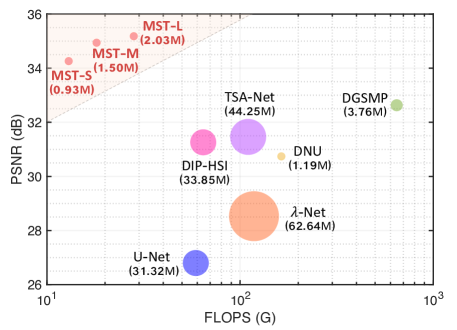
Figure 1: PSNR-Params-FLOPS comparisons with CNN-based HSI reconstruction methods. The vertical axis is PSNR (in dB performance), the horizontal axis is FLOPS (computational cost), and the circle radius is Params (memory cost). Our proposed Mask-guided Spectral-wise Transformers (MSTs) outperform previous methods while requiring significantly cheaper FLOPS and Params.

Hyperspectral imaging refers to multi-channel imaging where each channel captures the information at a specific spectral wavelength for a real-world scene. Generally, hyperspectral images (HSIs) have more spectral bands than normal RGB images to store richer information and delineate more detailed characteristics of the imaged scene. Relying on this property, HSIs have been widely applied to many computer vision related tasks, e.g., remote sensing [5, 34, 59], object tracking [21, 40], medical image processing [3, 33, 37], etc. To collect HSIs, conventional imaging systems with spectrometers scan the scenes along the spatial or spectral dimension, usually requiring a long time. Therefore, these traditional imaging systems are unsuitable for capturing and measuring dynamic scenes. Recently, researchers have used snapshot compressive imaging (SCI) systems to capture HSIs. These SCI systems compress information of snapshots along the spectral dimension into one single 2D measurement [58]. Among current existing SCI systems [32, 45, 47, 10, 16], the coded aperture snapshot spectral imaging (CASSI) [36, 45] stands out and forms one promising mainstream research direction.

Based on CASSI, a large number of reconstruction algorithms have been proposed to recover the 3D HSI cube from the 2D measurement. Conventional model-based methods adopt hand-crafted priors such as sparsity [23, 29, 46], total variation [24, 51, 57], and non-local similarity [30, 52, 61] to regularize the reconstruction procedure. However, these methods need to tweak parameters manually, resulting in poor generalization ability, unsatisfactory reconstruction quality, and slow restoration speed. With the development of deep learning, HSI reconstruction has witnessed significant progress. Deep convolutional neural network (CNN) applies a powerful model to learn the end-to-end mapping function from the 2D measurement to the 3D HSI cube. Although impressive results have been achieved, CNN-based methods [39, 36, 20, 35] show limitations in modeling the inter-spectra similarity and long-range dependencies. Besides, the HSIs are modulated by a physical mask in CASSI. Nonetheless, previous CNN-based methods [36, 48, 35, 38] mainly adopt the inner product between the mask and the shifted measurement as the input. This scheme corrupts the input HSI information and does not fully explore the guidance effect of the mask, leading to limited improvement.

In recent years, the natural language processing (NLP) model, Transformer [44], has been introduced into computer vision and outperformed CNN methods in many tasks. The Multi-head Self-Attention (MSA) module in Transformer excels at capturing non-local similarity and long-range dependencies. This advantage provides a possibility to address the aforementioned limitations of CNN-based methods in HSI reconstruction. However, directly applying the original Transformer may be unsuitable for HSI restoration due to the following reasons. Firstly, original Transformers learn to capture the long-range dependencies in spatial wise but the representations of HSIs are spectrally highly self-similar. In this case, the inter-spectra similarity and correlations are not well modeled. Meanwhile, the spectral information is spatially sparse. Capturing spatial interactions may be less cost-effective than modeling spectral correlations with the same resources. Secondly, the HSI representations are modulated by the mask in the CASSI system. The original Transformer without sufficient guidance may easily attend to many low-fidelity and less informative image regions when calculating self-attention. This may degrade the model efficiency. Thirdly, when using the original global Transformer [15], the computational complexity is quadratic to the spatial size. This burden is nontrivial and sometimes unaffordable. When using the local window-based Transformer [31], the receptive fields of the MSA module are limited within the position-specific windows and some highly related tokens may be neglected.

To cope with the above problems, we propose a novel method, Mask-guided Spectral-wise Transformer (MST), for HSI reconstruction. Firstly, in Fig. 2 (a), we observe that each spectral channel of HSIs captures an incomplete part of the same scene due to the constraints of the specific wavelength. This indicates that the HSI representations are similar and complementary along the spectral dimension. Hence, we propose a Spectral-wise MSA (S-MSA) to capture the long-range inter-spectra dependencies. Specifically, S-MSA treats each spectral channel feature as a token and calculates the self-attention along the spectral dimension. Secondly, in Fig. 2 (b), a mask is used in the CASSI system to modulate HSIs. The light transmittance of different positions on the mask varies significantly. This indicates that the fidelity of the modulated spectral information is position-sensitive. Therefore, we exploit the mask as a key clue and present a novel Mask-guided Mechanism (MM) that directs the S-MSA module to pay attention to the regions with high-fidelity spectral representations. Meanwhile, MM also alleviates the limitation of S-MSA in modeling the spatial correlations of HSI representations. Finally, with our proposed techniques, we establish a series of extremely efficient MST models that surpass state-of-the-art (SOTA) methods by a large margin, as illustrated in Fig. 1.

Our contributions can be summarized as follows:

• We propose a new method, MST, for HSI reconstruction. To the best of our knowledge, it is the first attempt to explore the potential of Transformer in this task.

• We present a novel self-attention, S-MSA, to capture the inter-spectra similarity and dependencies of HSIs.

• We customize an MM that directs S-MSA to pay attention to regions with high-fidelity HSI representations.

• Our MST dramatically outperforms SOTA methods on all scenes in simulation while requiring much cheaper Params and FLOPS. Besides, MST yields more visually pleasant results in real-world HSI reconstruction.

2 Related Work

2.1 HSI Reconstruction

Traditional HSI reconstruction methods [23, 29, 46, 30, 52, 61, 57, 43, 18] are mainly based on hand-crafted priors. For example, GAP-TV [57] introduces the total variation prior. DeSCI [30] exploits the low-rank property and non-local self-similarity. However, these model-based methods achieve unsatisfactory performance and generality due to the poor representing capacity. Recently, deep CNNs have been applied to learn the end-to-end mapping function of HSI reconstruction [39, 49, 20, 36, 19] to achieve promising performance. TSA-Net [36] uses three spatial-spectral self-attention modules to capture the dependencies in compressed spatial or spectral dimensions. The additional costs are nontrivial while the improvement is limited. DGSMP[20] suggests an interpretable HSI restoration method with learned Gaussian Scale Mixture (GSM) prior. These CNN-based methods yield impressive performance but show limitations in modeling inter-spectra similarity and correlations. Besides, the guidance effect of the mask is under-studied.

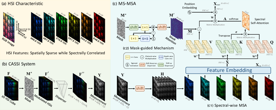
Figure 2: Illustration of the proposed method. Our Mask-guided Spectral-wise Multi-head Self-Attention (MS-MSA) is motivated by the HSI characteristics and CASSI system. (a) The representations of HSIs are spatially sparse while spectrally correlated. (b) The CASSI system uses a mask to modulate the HSIs. (c) Our MS-MSA in stage 0 of MST. (c1) S-MSA treats each spectral feature as a token and calculates self-attention along the spectral dimension. (c2) Mask-guided Mechanism directs the Spectral-wise MSA to pay attention to spatial regions with high-fidelity HSI representations. Some components are omitted for simplification. Please refer to the text for details.

2.2 Vision Transformer

Transformer is firstly proposed by [44] for machine translation. Recently, Transformer has achieved great success in many high-level vision tasks, such as image classification [31, 2, 15, 17], object detection [64, 1, 60, 13], segmentation [55, 8, 63], human pose estimation [26, 56, 7, 25], etc. Due to its promising performance, Transformer has also been introduced into low-level vision [11, 27, 9, 54, 6, 28, 14]. SwinIR [27] uses Swin Transformer [27] blocks to build up a residual network and achieve SOTA results in image restoration. However, these Transformers mainly aim to capture long-range dependencies of spatial regions. As for spectrally self-similar and mask-modulated HSIs, directly applying previous Transformers may be less effective in capturing spectral-wise correlations. In addition, the MSA may pay attention to less informative spatial regions.

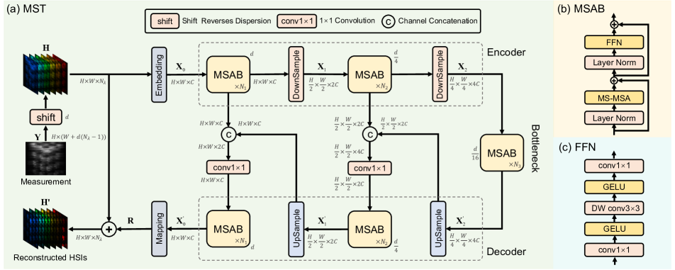
Figure 3: The overall architecture of MST. (a) MST adopts a U-shaped structure that consists of an encoder, a bottleneck, and a decoder. (b) MSAB is composed of a Feed-Forward Network (FFN), an MS-MSA, and two layer normalization. (c) The components of FFN.

3 CASSI System

A concise CASSI principle is shown in Fig. 2 (b). Given a 3D HSI cube, denoted by $\mathbf{F}\in\mathbb{R}^{H\times W\times N_{\lambda}}$, where $H$, $W$, and $N_{\lambda}$ represent the HSI’s height, width, and number of wavelengths, respectively. $\mathbf{F}$ is firstly modulated by the coded aperture (physical mask) $\mathbf{M^{*}}\in\mathbb{R}^{H\times W}$ as

$$\mathbf{F}^{\prime}(:,:,n_{\lambda})=\mathbf{F}(:,:,n_{\lambda})\odot\mathbf{M^{*}},\vspace{-1.2mm}$$ (1)

where $\mathbf{F}^{\prime}$ denotes the modulated HSIs, $n_{\lambda}\in[1,\dots,N_{\lambda}]$ indexes the spectral channels, and $\odot$ denotes the element-wise multiplication. After passing through the disperser, $\mathbf{F}^{\prime}$ becomes tilted and is considered to be sheared along the $y$-axis. We use $\mathbf{F}^{\prime\prime}\in\mathbb{R}^{H\times(W+d(N_{\lambda}-1))\times N_{\lambda}}$ to denote the tilted HSI cube, where $d$ represents the shifting step. We assume $\lambda_{c}$ to be the reference wavelength, i.e., $\mathbf{F}^{\prime\prime}(:,:,n_{\lambda_{c}})$ is not sheared along the $y$-axis. Then we have

$$\mathbf{F}^{\prime\prime}(u,v,n_{\lambda})=\mathbf{F}^{\prime}(x,y+d(\lambda_{n}-\lambda_{c}),n_{\lambda}),\vspace{-1.2mm}$$ (2)

where $(u,v)$ represents the coordinate system on the detector plane, $\lambda_{n}$ denotes the wavelength of the $n_{\lambda}$-th channel, and $d(\lambda_{n}-\lambda_{c})$ indicates the spatial shifting for the $n_{\lambda}$-th channel on $\mathbf{F}^{\prime\prime}$. Finally, the captured 2D compressed measurement $\mathbf{Y}\in\mathbb{R}^{H\times(W+d(N_{\lambda}-1))}$ can be obtained by

$$\mathbf{Y}=\sum_{n_{\lambda}=1}^{N_{\lambda}}\mathbf{F}^{\prime\prime}(:,:,n_{\lambda})+\mathbf{G},\vspace{-1.5mm}$$ (3)

where $\mathbf{G}\in\mathbb{R}^{H\times(W+d(N_{\lambda}-1))}$ is the imaging noise on the measurement, generated by the photon sensing detector.

4 Method

4.1 Overall Architecture

The overall architecture of MST is shown in Fig. 3 (a). We adopt a U-shaped structure that consists of an encoder, a bottleneck, and a decoder. MST is built up by Mask-guided Spectral-wise Attention Blocks (MSAB). Firstly, we reverse the dispersion process (Eq. (2)) and shift back the measurement to obtain the initialized signal $\mathbf{H}\in\mathbb{R}^{H\times W\times N_{\lambda}}$ as

$$\mathbf{H}(x,y,n_{\lambda})=\mathbf{Y}(x,y-d(\lambda_{n}-\lambda_{c})).\vspace{-1.2mm}$$ (4)

Then we feed $\mathbf{H}$ into the model. Firstly, MST exploits a conv3$\times$3 (convolution with kernel size = 3) layer to map $\mathbf{H}$ into feature $\mathbf{X}_{0}\in\mathbb{R}^{H\times W\times C}$. Secondly, $\mathbf{X}_{0}$ undergoes $N_{1}$ MSABs, a downsample module, $N_{2}$ MSABs, and a downsample module to generate hierarchical features. The downsample module is a strided conv4$\times$4 layer that downscales the feature maps and doubles the channels. Therefore, the feature of the $i$-th stage of the encoder is denoted as $\mathbf{X}_{i}\in\mathbb{R}^{\frac{H}{2^{i}}\times\frac{W}{2^{i}}\times 2^{i}C}$. Thirdly, $\mathbf{X}_{2}$ passes through the bottleneck that consists of $N_{3}$ MSABs. Subsequently, We follow the spirit of U-Net [42] and design a symmetrical structure as the decoder. In particular, the upsample module is a strided deconv2$\times$2 layer. The skip connections are exploited for feature aggregation between the encoder and decoder to alleviate the information loss caused by the downsample operations. Similarly, the feature of the $i$-th stage of the decoder is denoted as $\mathbf{X}^{\prime}_{i}\in\mathbb{R}^{\frac{H}{2^{i}}\times\frac{W}{2^{i}}\times 2^{i}C}$. After passing through the decoder, the feature maps undergo a conv3$\times$3 layer to generate the residual HSIs $\mathbf{R}\in\mathbb{R}^{H\times W\times N_{\lambda}}$. Finally, the reconstructed HSIs $\mathbf{H}^{\prime}\in\mathbb{R}^{H\times W\times N_{\lambda}}$ can be obtained by the sum of $\mathbf{R}$ and $\mathbf{H}$, i.e., $\mathbf{H}^{\prime}=\mathbf{H}+\mathbf{R}$.

In implementation, we set $C$ to 28 and change the combination $(N_{1},N_{2},N_{3})$ to establish a series of MST models with small, medium, and large model sizes and computation costs: MST-S (2,2,2), MST-M (2,4,4), and MST-L (4,7,5).

The basic unit of MST is MSAB. As shown in Fig. 3 (b), MSAB consists of two layer normalization, a Mask-guided Spectral-wise MSA (MS-MSA), and a Feed-Forward Network (FFN). The details of FFN are depicted in Fig. 3 (c).

4.2 Spectral-wise Multi-head Self-Attention

The non-local self-similarity is often exploited in HSI reconstruction but is usually not well modeled by CNN-based methods. Due to the effectiveness of Transformer in capturing non-local long-range dependencies and its impressive performance in other vision tasks, we aim to explore the potential of Transformer in HSI reconstruction. However, there are two main issues when directly applying Transformer to HSI restoration. The first problem is that original Transformers model long-range dependencies in spatial dimensions. But the HSI representations are spatially sparse and spectrally correlated, as shown in Fig. 2 (a). Capturing spatial-wise interactions may be less cost-effective than modeling spectral-wise correlations. Hence, we propose S-MSA that treats each spectral feature map as a token and calculates self-attention along the spectral dimension. Fig. 2 (c1) shows the S-MSA used in stage 0 of MST. The input $\mathbf{X}_{in}\in\mathbb{R}^{H\times W\times C}$ is reshaped into tokens $\mathbf{X}\in\mathbb{R}^{HW\times C}$. Then $\mathbf{X}$ is linearly projected into query $\mathbf{Q}\in\mathbb{R}^{HW\times C}$, key $\mathbf{K}\in\mathbb{R}^{HW\times C}$, and value $\mathbf{V}\in\mathbb{R}^{HW\times C}$:

$$\mathbf{Q}=\mathbf{X}\mathbf{W}^{\mathbf{Q}},\mathbf{K}=\mathbf{X}\mathbf{W}^{\mathbf{K}},\mathbf{V}=\mathbf{X}\mathbf{W}^{\mathbf{V}},\vspace{0.2mm}$$ (5)

where $\mathbf{W}^{\mathbf{Q}}$, $\mathbf{W}^{\mathbf{K}}$, and $\mathbf{W}^{\mathbf{V}}\in\mathbb{R}^{C\times C}$ are learnable parameters; $biases$ are omitted for simplification. Subsequently, we respectively split $\mathbf{Q}$, $\mathbf{K}$, and $\mathbf{V}$ into $N$ heads along the spectral channel dimension: $\mathbf{Q}=[\mathbf{Q}_{1},\ldots,\mathbf{Q}_{N}]$, $\mathbf{K}=[\mathbf{K}_{1},\ldots,\mathbf{K}_{N}]$, and $\mathbf{V}=[\mathbf{V}_{1},\ldots,\mathbf{V}_{N}]$. The dimension of each head is $d_{h}=\frac{C}{N}$. Please note that Fig. 2 (c1) depicts the situation with $N$ = 1 and some details are omitted for simplification. Different from original MSAs, our S-MSA treats each spectral representation as a token and calculates the self-attention for each $head_{j}$:

$$\mathbf{A}_{j}=\text{softmax}(\sigma_{j}\mathbf{K}_{j}^{\text{T}}\mathbf{Q}_{j}),~{}~{}{head}_{j}=\mathbf{V}_{j}\mathbf{A}_{j},\vspace{-0.2mm}$$ (6)

where $\mathbf{K}_{j}^{\text{T}}$ denotes the transposed matrix of $\mathbf{K}_{j}$. Because the spectral density varies significantly with respect to the wavelengths, we use a learnable parameter $\sigma_{j}\in\mathbb{R}^{1}$ to adapt the self-attention $\mathbf{A}_{j}$ by re-weighting the matrix multiplication $\mathbf{K}_{j}^{\text{T}}\mathbf{Q}_{j}$ inside $head_{j}$. Subsequently, the outputs of $N$ heads are concatenated in spectral wise to undergo a linear projection and then is added with a position embedding:

$$\text{S-MSA}(\mathbf{X})=\big{(}\mathop{\text{Concat}}\limits_{j=1}^{N}(head_{j})\big{)}\mathbf{W}+f_{p}(\mathbf{V}),$$ (7)

where $\mathbf{W}\in\mathbb{R}^{C\times C}$ are learnable parameters, $f_{p}(\cdot)$ is the function to generate position embedding. It consists of two depth-wise conv3$\times$3 layers, a GELU activation, and reshape operations. The HSIs are sorted by the wavelength along the spectral dimension. Therefore, we exploit this embedding to encode the position information of different spectral channels. Finally, we reshape the result of Eq. (7) to obtain the output feature maps $\mathbf{X}_{out}\in\mathbb{R}^{H\times W\times C}$.

We analyze the computational complexity of S-MSA and compare it with other MSAs. We only compare the main difference, i.e., the self-attention mechanism in Eq. (6):

$$O(\text{S-MSA})=\frac{2HWC^{2}}{N},~{}O(\text{G-MSA})=2(HW)^{2}C,$$ (8)

$$O(\text{W-MSA})=2(M^{2})^{2}(\frac{HW}{M^{2}})C=2M^{2}HWC,$$

where G-MSA denotes the original global MSA [15], W-MSA denotes the local window-based MSA [31], and $M$ represents the window size. The computational complexity of S-MSA and W-MSA is linear to the spatial size $HW$. This cost is much cheaper than that of G-MSA (quadratic to $HW$). Meanwhile, S-MSA treats a whole spectral feature map as a token. Thus, the receptive field of our S-MSA is global and not limited to position-specific windows.

4.3 Mask-guided Mechanism

The second problem of directly using Transformer for HSI restoration is that original Transformers may attend to some less informative spatial regions with low-fidelity HSI representations. In CASSI, a physical mask is used to modulate the HSIs. Thus, the light transmittance of different positions on the mask varies. As a result, the fidelity of the modulated spectral information is position-sensitive. This observation motivates us that the mask should be used as a clue to direct the model to attend to regions with high-fidelity HSI representations. In this part, we firstly analyze the usage of the mask in previous CNN-based methods, and then introduce our Mask-guided Mechanism (MM).

Previous Mask Usage Scheme. Previous CNN-based methods [36, 48, 35, 38] mainly conduct an inner product between the initialized HSIs $\mathbf{H}$ and the mask $\mathbf{M}^{*}$ to generate a modulated input. This scheme introduces spatial fidelity information but suffers from the following limitations: (i) This operation corrupts the input HSI representations, causes the information loss, and leads to spatial discontinuity. (ii) This scheme only operates at the input. The guidance effect of the mask in directing the network to pay attention to regions with high-fidelity HSI representations is not fully explored. (iii) This scheme does not exploit learnable parameters to model the spatial-wise correlations.

Our MM. Different from previous methods, our MM preserves all the input HSI representations and learns to direct S-MSA to pay attention to the spatial regions with high-fidelity spectral representations. To be specific, given the mask $\mathbf{M}^{*}\in\mathbb{R}^{H\times W}$ shown in Fig. 2 (c2), since the modulated HSIs are shifted by the disperser of the CASSI system, we firstly shift $\mathbf{M}^{*}$ like the dispersion process:

$$\mathbf{M}_{s}(x,y,n_{\lambda})=\mathbf{M}^{*}(x,y+d(\lambda_{n}-\lambda_{c})),\vspace{-0.8mm}$$ (9)

where $\mathbf{M}_{s}\in\mathbb{R}^{H\times(W+d(N_{\lambda}-1))\times N_{\lambda}}$ denotes the shifted version of $\mathbf{M}^{*}$. The shifted regions out of the range in $y$-axis on $\mathbf{M}^{*}$ are set to 0. Please note that Fig. 2 (c2) shows the MM used in stage 0 of MST. To match the scale of the feature maps in stage $i$ of MST, $\mathbf{M}_{s}$ needs to pass through the same downsample operations in Fig. 3 (a). Subsequently, $\mathbf{M}_{s}$ undergoes a conv1$\times$1 layer and then is input to two paths. The upper path is an identity mapping to retain the original fidelity information. The lower path undergoes a conv1$\times$1 layer, a depth-wise conv5$\times$5 layer, a sigmoid activation, and an inner product with the upper path. S-MSA is effective in capturing inter-spectra dependencies but shows limitations in modeling spatial interactions of HSI representations. Thus, the lower path is designed to capture the spatial-wise correlations. Then we have

$$\mathbf{M}^{\prime}_{s}=(\mathbf{W}_{1}\mathbf{M}_{s})\odot(1+\delta(f_{dw}(\mathbf{W}_{2}\mathbf{W}_{1}\mathbf{M}_{s})),$$ (10)

where $\mathbf{W}_{1}$ and $\mathbf{W}_{2}$ are the learnable parameters of the two conv1$\times$1 layers, $f_{dw}(\cdot)$ denotes the mapping function of the depth-wise conv5$\times$5 layer, $\delta(\cdot)$ represents the sigmoid activation, and $\mathbf{M}^{\prime}_{s}\in\mathbb{R}^{H\times(W+d(N_{\lambda}-1))\times C}$ denotes the intermediate feature maps. To spatially align the mask attention map with the modulated HSIs $\mathbf{F}^{\prime}$ in the CASSI system (Fig. 2 (b)) and the initialized input $\mathbf{H}$ of MST (Fig. 3 (a)), we reverse the dispersion process and shift back $\mathbf{M}^{\prime}_{s}$ to obtain the mask attention map $\mathbf{M}^{\prime}\in\mathbb{R}^{H\times W\times C}$ as

$$\mathbf{M}^{\prime}(x,y,n_{\lambda})=\mathbf{M}^{\prime}_{s}(x,y-d(\lambda_{n}-\lambda_{c}),n_{\lambda}),\vspace{-1.4mm}$$ (11)

where $n_{\lambda}\in[1,\dots,C]$ indexes the spectral channels to match the dimensions of $\mathbf{M}^{\prime}_{s}$. We reshape $\mathbf{M}^{\prime}$ into $\mathbf{M}\in\mathbb{R}^{HW\times C}$ to match the dimensions of $\mathbf{V}$. Then we split $\mathbf{M}$ into $N$ heads in spectral wise: $\mathbf{M}=[\mathbf{M}_{1},\ldots,\mathbf{M}_{N}]$. For each $head_{j}$, MM conducts its guidance by re-weighting $\mathbf{V}_{j}$ using $\mathbf{M}_{j}\in\mathbb{R}^{HW\times d_{h}}$. Hence, when using MM to direct S-MSA, the S-MSA module just needs to make a simple modification by re-formulating $head_{j}$ in Eq. (6):

$${head}_{j}=(\mathbf{M}_{j}\odot\mathbf{V}_{j})\mathbf{A}_{j}.\vspace{-1.2mm}$$ (12)

The subsequent steps of S-MSA remain unchanged. By using MM, S-MSA can extract non-corrupted HSI representations, enjoy the guidance of position-sensitive fidelity information, and adaptively model the spatial-wise interactions.

	TwIST [4]		GAP-TV [57]		DeSCI [30]		$\lambda$-net [39]		HSSP [49]		DNU [50]		DIP-HSI [38]		TSA-Net [36]		DGSMP [20]		MST-S		MST-M		MST-L
Scene	PSNR	SSIM	PSNR	SSIM	PSNR	SSIM	PSNR	SSIM	PSNR	SSIM	PSNR	SSIM	PSNR	SSIM	PSNR	SSIM	PSNR	SSIM	PSNR	SSIM	PSNR	SSIM	PSNR	SSIM
1	25.16	0.700	26.82	0.754	27.13	0.748	30.10	0.849	31.48	0.858	31.72	0.863	32.68	0.890	32.03	0.892	33.26	0.915	34.71	0.930	35.15	0.937	35.40	0.941
2	23.02	0.604	22.89	0.610	23.04	0.620	28.49	0.805	31.09	0.842	31.13	0.846	27.26	0.833	31.00	0.858	32.09	0.898	34.45	0.925	35.19	0.935	35.87	0.944
3	21.40	0.711	26.31	0.802	26.62	0.818	27.73	0.870	28.96	0.823	29.99	0.845	31.30	0.914	32.25	0.915	33.06	0.925	35.32	0.943	36.26	0.950	36.51	0.953
4	30.19	0.851	30.65	0.852	34.96	0.897	37.01	0.934	34.56	0.902	35.34	0.908	40.54	0.962	39.19	0.953	40.54	0.964	41.50	0.967	42.48	0.973	42.27	0.973
5	21.41	0.635	23.64	0.703	23.94	0.706	26.19	0.817	28.53	0.808	29.03	0.833	29.79	0.900	29.39	0.884	28.86	0.882	31.90	0.933	32.49	0.943	32.77	0.947
6	20.95	0.644	21.85	0.663	22.38	0.683	28.64	0.853	30.83	0.877	30.87	0.887	30.39	0.877	31.44	0.908	33.08	0.937	33.85	0.943	34.28	0.948	34.80	0.955
7	22.20	0.643	23.76	0.688	24.45	0.743	26.47	0.806	28.71	0.824	28.99	0.839	28.18	0.913	30.32	0.878	30.74	0.886	32.69	0.911	33.29	0.921	33.66	0.925
8	21.82	0.650	21.98	0.655	22.03	0.673	26.09	0.831	30.09	0.881	30.13	0.885	29.44	0.874	29.35	0.888	31.55	0.923	31.69	0.933	32.40	0.943	32.67	0.948
9	22.42	0.690	22.63	0.682	24.56	0.732	27.50	0.826	30.43	0.868	31.03	0.876	34.51	0.927	30.01	0.890	31.66	0.911	34.67	0.939	35.35	0.942	35.39	0.949
10	22.67	0.569	23.10	0.584	23.59	0.587	27.13	0.816	28.78	0.842	29.14	0.849	28.51	0.851	29.59	0.874	31.44	0.925	31.82	0.926	32.53	0.935	32.50	0.941
Avg	23.12	0.669	24.36	0.669	25.27	0.721	28.53	0.841	30.35	0.852	30.74	0.863	31.26	0.894	31.46	0.894	32.63	0.917	34.26	0.935	34.94	0.943	35.18	0.948

Table 1: Quantitative results on 10 scenes in simulation. PSNR and SSIM are reported. MSTs significantly surpass other competitors.

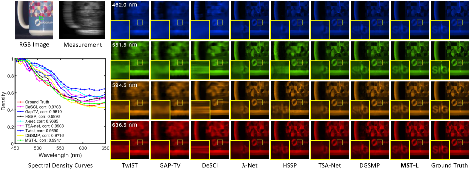
Figure 4: Reconstructed simulation HSI comparisons of Scene 5 with 4 out of 28 spectral channels. 7 SOTA algorithms and our MST-L are included. The spectral curves (bottom-left) are corresponding to the selected green box of the RGB image. Zoom in for a better view.

5 Experiments

5.1 Experimental Settings

Following the settings of TSA-Net [36], we adopt 28 wavelengths from 450 nm to 650 nm derived by spectral interpolation manipulation for HSIs. We perform experiments on both simulation and real HSI datasets.

Simulation HSI Data. We use two simulation hyperspectral image datasets, CAVE [41] and KAIST [12]. CAVE dataset is composed of 32 hyperspectral images at a spatial size of 512$\times$512. KAIST dataset consists of 30 hyperspectral images at a spatial size of 2704$\times$3376. Following the schedule of TSA-Net [36], we adopt CAVE as the training set. 10 scenes from KAIST are selected for testing.

Real HSI Data. We use the real HSI dataset collected by the CASSI system developed in TSA-Net [36].

Evaluation Metrics. We adopt peak signal-to-noise ratio (PSNR) and structural similarity (SSIM) [53] as the metrics to evaluate the HSI reconstruction performance.

Implementation Details. We implement MST in Pytorch. All the models are trained with Adam [22] optimizer ($\beta_{1}$ = 0.9 and $\beta_{2}$ = 0.999) for 300 epochs. The learning rate is set to 4$\times$10^-4 in the beginning and is halved every 50 epochs during the training procedure. When conducting experiments on simulation data, patches at a spatial size of 256$\times$256 cropped from the 3D cubes are fed into the networks. As for real hyperspectral image reconstruction, the patch size is set to 660$\times$660 to match the real-world measurement. The shifting step $d$ in dispersion is set to 2. Thus, the measurement sizes are 256$\times$310 and 660$\times$714 for simulation and real HSI datasets. The shifting step in reversed dispersion is ${d}/{4^{i}},i=0,1,2$ for the $i$-th stage of MST. The batch size is 5. Random flipping and rotation are used for data augmentation. The models are trained on one RTX 8000 GPU. The training objective is to minimize the Root Mean Square Error (RMSE) and Spectrum Constancy Loss [62] between the reconstructed and ground-truth HSIs.

Figure 5: Reconstructed real HSI comparisons of Scene 3 with 4 out of 28 spectral channels. Seven SOTA algorithms and our MST-L are included. MST-L reconstructs more detailed contents and suppresses more noise. Please zoom in for better visualization performance.

5.2 Quantitative Results

We compare our MST with several SOTA HSI reconstruction algorithms, including three model-based methods (TwIST [4], GAP-TV [57], and DeSCI [30]) and six CNN-based methods ($\lambda$-net [39], HSSP [49], DNU [50], PnP-DIP-HSI [38], TSA-Net [36], and DGSMP [20]). For fair comparisons, all methods are tested with the same settings as DGSMP [20]. The PSNR and SSIM results of different methods on 10 scenes in the simulation datasets are listed in Tab. 1. The Params and FLOPS (test size = 256$\times$256) of open-source CNN-based algorithms are reported in Tab. LABEL:tab:model_size. It can be observed from these two tables that our MSTs significantly surpass previous methods by a large margin on all the 10 scenes while requiring much cheaper memory and computational costs. More specifically, our best model, MST-L surpasses DGSMP, TSA-Net, and $\lambda$-net by 2.55, 3.72, and 6.65 dB while costing 54.0% (2.03 / 3.76), 4.6%, and 3.2% Params and 4.4% (28.15 / 646.65), 25.6%, and 23.9% FLOPS. Surprisingly, even our smallest model, MST-S outperforms DGSMP, TSA-Net, PnP-DIP-HSI, DNU, and $\lambda$-net by 1.63, 2.80, 3.00, 3.52, and 5.73 dB while requiring 24.7%, 2.1%, 2.7%, 78.2%, and 1.5% Params and 2.0%, 11.8%, 20.1%, 7.9%, and 11.0% FLOPS.

To intuitively show the superiority of our MST, we provide PSNR-Params-FLOPS comparisons of different reconstruction algorithms in Fig. 1. The vertical axis is PSNR (performance), the horizontal axis is FLOPS (computational cost), and the circle radius is Params (memory cost). It can be seen that our MSTs take up the upper-left corner, exhibiting the extreme efficiency advantages of our method.

5.3 Qualitative Results

Simulation HSI Reconstruction. Fig. 4 visualizes the reconstructed simulation HSIs of Scene 5 with 4 out of 28 spectral channels using seven SOTA methods and our MST-L. Please zoom in for a better view. As can be seen from the reconstructed HSIs (right) and the zoom-in patches of the selected yellow boxes, previous methods are less favorable to restore HSI details. They either yield over-smooth results sacrificing fine-grained structural contents and textural details, or introduce undesirable chromatic artifacts and blotchy textures. In contrast, our MST-L is more capable of producing perceptually-pleasing and sharp images, and preserving the spatial smoothness of the homogeneous regions. This is mainly because our MST-L enjoys the guidance of modulation information and captures the long-range dependencies of different spectral channels. In addition, we plot the spectral density curves (bottom-left) corresponding to the picked region of the green box in the RGB image (top-left). The highest correlation and coincidence between our curve and the ground truth demonstrate the spectral-wise consistency restoration effectiveness of our MST.

Real HSI Reconstruction. We further apply our proposed approach to real HSI reconstruction. Similar to [36, 20], we re-train our model (MST-L) on all scenes of CAVE [41] and KAIST [12] datasets. To simulate real imaging situations, we inject 11-bit shot noise into the measurements during training. Visual comparisons are shown in Fig. 5. Our MST-L surpasses previous algorithms in terms of high-frequency structural detail reconstruction and real noise suppression.

Baseline	S-MSA	MM	PSNR	SSIM	Params (M)	FLOPS (G)
✓			32.29	0.897	0.53	7.43
✓	✓		33.18	0.923	0.70	10.36
✓	✓	✓	34.26	0.935	0.93	12.96

(a)

Method	Baseline	Global MSA	Local W-MSA	Swin W-MSA	S-MSA
PSNR	32.29	32.67	32.75	32.86	33.18
SSIM	0.897	0.912	0.916	0.919	0.923
Params (M)	0.53	0.70	0.70	0.70	0.70
FLOPS (G)	7.43	11.88	11.07	11.07	10.36

(b)

Method	$\lambda$-net [39]	DNU [50]	DIP-HSI [38]	TSA-Net [36]	DGSMP [20]	MST-S	MST-M	MST-L
PSNR	28.53	30.74	31.26	31.46	32.63	34.26	34.94	35.18
SSIM	0.841	0.863	0.894	0.894	0.917	0.935	0.943	0.948
Params (M)	62.64	1.19	33.85	44.25	3.76	0.93	1.50	2.03
FLOPS (G)	117.98	163.48	64.42	110.06	646.65	12.96	18.07	28.15

(c)

Method	Input	MM	PSNR	SSIM
A	$\mathbf{H}$		33.18	0.923
B	$\mathbf{H}\odot\mathbf{M}^{*}$		33.57	0.927
C	$\mathbf{H}$	✓	34.26	0.935
D	$\mathbf{H}\odot\mathbf{M}^{*}$	✓	34.07	0.932

(d)

Table 2: Ablations. We train models on CAVE [41] and test on KAIST [12] in simulation. PSNR, SSIM, Params, and FLOPS are reported.

5.4 Ablation Study

In this part, we adopt the simulation HSI datasets [41, 12] to conduct ablation studies. The baseline model is derived by removing our S-MSA and MM from MST-S.

Break-down Ablation. We firstly conduct a break-down ablation experiment to investigate the effect of each component towards higher performance. The results are listed in Tab. LABEL:tab:breakdown. The baseline model yields 32.29 dB. When we successively apply our S-MSA and MM, the model continuously achieves 0.89 and 1.08 dB improvements. These results suggest the effectiveness of S-MSA and MM.

Self-Attention Scheme Comparison. We compare S-MSA with other self-attentions and report the results in Tab. LABEL:tab:attention. For fair comparisons, the Params of models using different self-attention schemes are set to the same value (0.70 M). Please note that we downscale the input feature of global MSA [15] into $\frac{1}{4}$ size to avoid out of memory. The baseline model yields 32.29 dB while costing 0.53 M Params and 7.43 G FLOPS.

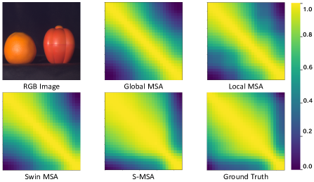
Figure 6: Visualization of the correlation coefficients among spectral channels of HSIs reconstructed by models using different MSAs. The correlation coefficient map of the model equipped with our S-MSA is the most similar one to that of the ground truth.

We respectively apply the global MSA [15], local window-based MSA [31], Swin W-MSA [31], and our S-MSA. The model gains by 0.38, 0.46, 0.57, and 0.89 dB while adding 4.45, 3.64, 3.64, and 2.93 G FLOPS. Our S-MSA yields the most significant improvement but requires the least computational cost. We explain these results by the HSI characteristics that the spectral representations are spatially sparse and spectrally highly self-similar. Hence, capturing spatial interactions may be less cost-effective than modeling inter-spectra dependencies. This evidence clearly verifies the efficiency superiority of our S-MSA.

In addition, we further conduct visual analysis about different MSAs in Fig. 6. Specifically, we visualize the correlation coefficients between each spectral pair of HSIs reconstructed by models equipped with different MSAs. It can be observed that the correlation coefficient map of the model using our proposed S-MSA is the most similar one to that of the ground truth. These results demonstrate the promising effectiveness of our S-MSA in modeling the inter-spectra similarity and long-range spectral-wise dependencies.

Mask-guided Mechanism. We conduct ablation studies to investigate the effect of the previous mask usage scheme described in Sec. 4.3, our MM, and their interaction. The adopted network is the baseline model using S-MSA. The results are reported in Tab. LABEL:tab:mask. Method A uses our input setting. Method B exploits the previous scheme that adopts $\mathbf{H}\odot\mathbf{M}^{*}$ as the input. B achieves a limited improvement due to the HSI representation corruption and under-utilization of the mask. Method C uses our MM. C yields the most significant improvement by 1.08 dB, showing the guidance advantage of MM for HSI reconstruction. D exploits both the previous scheme and our MM but degrades by 0.19 dB when compared to method C. This degradation may stem from the loss of some input spectral information.

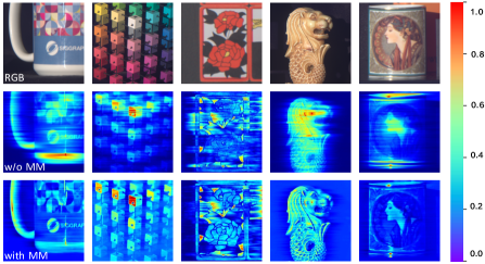
Figure 7: Visual analysis of the feature maps of the last MSAB in MST-S. The top row shows the original RGB images. The middle and bottom rows exhibit the feature maps without and with MM. The model using MM pays more high-fidelity attention to details.

Additionally, to intuitively show the advantages of MM, we visualize the feature maps of the last MSAB in MST-S. As depicted in Fig. 7, the top row shows the original RGB images. The middle and bottom rows respectively exhibit the feature maps without and with MM. It can be clearly observed that the model without MM generates blurred, distorted, and incomplete feature maps while sacrificing some details, neglecting some scene patches, or introducing unpleasant artifacts. In contrast, the model using our MM pays more accurate and high-fidelity attention to the detailed contents and structural textures of the desired scenes.

6 Conclusion

In this paper, we propose an efficient Transformer-based framework, MST, for accurate HSI reconstruction. Motivated by the HSI characteristics, we develop an S-MSA to capture inter-spectra similarity and dependencies. Moreover, we customize an MM module to direct S-MSA to pay attention to spatial regions with high-fidelity HSI representations. With these novel techniques, we establish a series of extremely efficient MST models. Quantitative experiments demonstrate that our method surpasses SOTA algorithms by a large margin, even requiring significantly cheaper Params and FLOPS. Qualitative comparisons show that our MST achieves more visually pleasant reconstructed HSIs.

Acknowledgements: This work is partially supported by the NSFC fund (61831014), the Shenzhen Science and Technology Project under Grant (ZDYBH201900000002, CJGJZD20200617102601004), the Westlake Foundation (2021B1501-2), and the funding from Lochn Optics.

References

- [1] Nicolas arion, Francisco Massa, Gabriel Synnaeve, Nicolas Usunier, Alexander Kirillov, and Sergey Zagoruyko. End-to-end object detection with transformers. In ECCV, 2020.
- [2] Anurag Arnab, Mostafa Dehghani, Georg Heigold, Chen Sun, Mario Lučić, and Cordelia Schmid. Vivit: A video vision transformer. arXiv preprint arXiv:2103.15691, 2021.
- [3] V. Backman, M. B. Wallace, L. Perelman, J. Arendt, R. Gurjar, M. Muller, Q. Zhang, G. Zonios, E. Kline, and T. McGillican. Detection of preinvasive cancer cells. Nature, 2000.
- [4] J.M. Bioucas-Dias and M.A.T. Figueiredo. A new twist: Two-step iterative shrinkage/thresholding algorithms for image restoration. TIP, 2007.
- [5] M. Borengasser, W. S. Hungate, and R. Watkins. Hyperspectral remote sensing: principles and applications. CRC press, 2007.
- [6] Yuanhao Cai, Xiaowan Hu, Haoqian Wang, Yulun Zhang, Hanspeter Pfister, and Donglai Wei. Learning to generate realistic noisy images via pixel-level noise-aware adversarial training. In NeurIPS, 2021.
- [7] Yuanhao Cai, Zhicheng Wang, Zhengxiong Luo, Binyi Yin, Angang Du, Haoqian Wang, Xinyu Zhou, Erjin Zhou, Xiangyu Zhang, and Jian Sun. Learning delicate local representations for multi-person pose estimation. arXiv preprint arXiv:2003.04030, 2020.
- [8] Hu Cao, Yueyue Wang, Joy Chen, Dongsheng Jiang, Xiaopeng Zhang, Qi Tian, and Manning Wang. Swin-unet: Unet-like pure transformer for medical image segmentation. arXiv preprint arXiv:2105.05537, 2021.
- [9] Jiezhang Cao, Yawei Li, Kai Zhang, and Luc Van Gool. Video super-resolution transformer. arXiv preprint arXiv:2106.06847, 2021.
- [10] Xun Cao, Tao Yue, Xing Lin, Stephen Lin, Xin Yuan, Qionghai Dai, Lawrence Carin, and David J. Brady. Computational snapshot multispectral cameras: Toward dynamic capture of the spectral world. IEEE Signal Processing Magazine, 2016.
- [11] Hanting Chen, Yunhe Wang, Tianyu Guo, Chang Xu, Yiping Deng, Zhenhua Liu, Siwei Ma, Chunjing Xu, Chao Xu, and Wen Gao. Pre-trained image processing transformer. In CVPR, 2021.
- [12] Inchang Choi, MH Kim, D Gutierrez, DS Jeon, and G Nam. High-quality hyperspectral reconstruction using a spectral prior. In Technical report, 2017.
- [13] Xiyang Dai, Yinpeng Chen, Jianwei Yang, Pengchuan Zhang, Lu Yuan, and Lei Zhang. Dynamic detr: End-to-end object detection with dynamic attention. In ICCV, 2021.
- [14] Zhuo Deng, Yuanhao Cai, Lu Chen, Zheng Gong, Qiqi Bao, Xue Yao, Dong Fang, Shaochong Zhang, and Lan Ma. Rformer: Transformer-based generative adversarial network for real fundus image restoration on a new clinical benchmark. arXiv preprint arXiv:2201.00466, 2022.
- [15] Alexey Dosovitskiy, Lucas Beyer, Alexander Kolesnikov, Dirk Weissenborn, Xiaohua Zhai, Thomas Unterthiner, Mostafa Dehghani, Matthias Minderer, Georg Heigold, Sylvain Gelly, Jakob Uszkoreit, and Neil Houlsby. An image is worth 16x16 words: Transformers for image recognition at scale. In ICLR, 2021.
- [16] Hao Du, Xin Tong, Xun Cao, and Stephen Lin. A prism-based system for multispectral video acquisition. In ICCV, 2009.
- [17] Alaaeldin El-Nouby, Hugo Touvron, Mathilde Caron, Piotr Bojanowski, Matthijs Douze, Armand Joulin, Ivan Laptev, Natalia Neverova, Gabriel Synnaeve, Jakob Verbeek, et al. Xcit: Cross-covariance image transformers. In NeurIPS, 2021.
- [18] Ying Fu, Yinqiang Zheng, Imari Sato, and Yoichi Sato. Exploiting spectral-spatial correlation for coded hyperspectral image restoration. In CVPR, 2016.
- [19] Xiaowan Hu, Yuanhao Cai, Jing Lin, Haoqian Wang, Xin Yuan, Yulun Zhang, Radu Timofte, and Luc Van Gool. Hdnet: High-resolution dual-domain learning for spectral compressive imaging. In CVPR, 2022.
- [20] Tao Huang, Weisheng Dong, Xin Yuan, Jinjian Wu, and Guangming Shi. Deep gaussian scale mixture prior for spectral compressive imaging. In CVPR, 2021.
- [21] M. H. Kim, T. A. Harvey, D. S. Kittle, H. Rushmeier, R. O. Prum J. Dorsey, and D. J. Brady. 3d imaging spectroscopy for measuring hyperspectral patterns on solid objects. ACM Transactions on on Graphics, 2012.
- [22] Diederik P. Kingma and Jimmy Lei Ba. Adam: A method for stochastic optimization. In ICLR, 2015.
- [23] David Kittle, Kerkil Choi, Ashwin Wagadarikar, and David J Brady. Multiframe image estimation for coded aperture snapshot spectral imagers. Applied optics, 2010.
- [24] David Kittle, Kerkil Choi, Ashwin Wagadarikar, and David J. Brady. Multiframe image estimation for coded aperture snapshot spectral imagers. OSA Applied Optics, 2010.
- [25] Ke Li, Shijie Wang, Xiang Zhang, Yifan Xu, Weijian Xu, and Zhuowen Tu. Pose recognition with cascade transformers. In CVPR, 2021.
- [26] Yanjie Li, Shoukui Zhang, Zhicheng Wang, Sen Yang, Wankou Yang, Shu-Tao Xia, and Erjin Zhou. Tokenpose: Learning keypoint tokens for human pose estimation. In ICCV, 2021.
- [27] Jingyun Liang, Jiezhang Cao, Guolei Sun, Kai Zhang, Luc Van Gool, and Radu Timofte. Swinir: Image restoration using swin transformer. In ICCVW, 2021.
- [28] Jing Lin, Yuanhao Cai, Xiaowan Hu, Haoqian Wang, Youliang Yan, Xueyi Zou, Henghui Ding, Yulun Zhang, Radu Timofte, and Luc Van Gool. Flow-guided sparse transformer for video deblurring. arXiv preprint arXiv:2201.01893, 2022.
- [29] Xing Lin, Yebin Liu, Jiamin Wu, and Qionghai Dai. Spatial-spectral encoded compressive hyperspectral imaging. TOG, 2014.
- [30] Yang Liu, Xin Yuan, Jinli Suo, David Brady, and Qionghai Dai. Rank minimization for snapshot compressive imaging. TPAMI, 2019.
- [31] Ze Liu, Yutong Lin, Yue Cao, Han Hu, Yixuan Wei, Zheng Zhang, Stephen Lin, and Baining Guo. Swin transformer: Hierarchical vision transformer using shifted windows. In ICCV, 2021.
- [32] Patrick Llull, Xuejun Liao, Xin Yuan, Jianbo Yang, David Kittle, Lawrence Carin, Guillermo Sapiro, and David J Brady. Coded aperture compressive temporal imaging. Optics Express, 2013.
- [33] Guolan Lu and Baowei Fei. Medical hyperspectral imaging: a review. Journal of Biomedical Optics, 2014.
- [34] Farid Melgani and Lorenzo Bruzzone. Classification of hyperspectral remote sensing images with support vector machines. IEEE Transactions on Geoscience and Remote Sensing, 2004.
- [35] Ziyi Meng, Shirin Jalali, and Xin Yuan. Gap-net for snapshot compressive imaging. arXiv preprint arXiv:2012.08364, 2020.
- [36] Ziyi Meng, Jiawei Ma, and Xin Yuan. End-to-end low cost compressive spectral imaging with spatial-spectral self-attention. In ECCV, 2020.
- [37] Ziyi Meng, Mu Qiao, Jiawei Ma, Zhenming Yu, Kun Xu, and Xin Yuan. Snapshot multispectral endomicroscopy. Optics Letters, 2020.
- [38] Ziyi Meng, Zhenming Yu, Kun Xu, and Xin Yuan. Self-supervised neural networks for spectral snapshot compressive imaging. In ICCV, 2021.
- [39] Xin Miao, Xin Yuan, Yunchen Pu, and Vassilis Athitsos. l-net: Reconstruct hyperspectral images from a snapshot measurement. In ICCV, 2019.
- [40] Z. Pan, G. Healey, M. Prasad, and B. Tromberg. Face recognition in hyperspectral images. TPAMI, 2003.
- [41] Jong-Il Park, Moon-Hyun Lee, Michael D. Grossberg, and Shree K. Nayar. Multispectral imaging using multiplexed illumination. In ICCV, 2007.
- [42] Olaf Ronneberger, Philipp Fischer, Thomas Brox, a, and b. U-net: Convolutional networks for biomedical image segmentation. In MICCAI, 2015.
- [43] Jin Tan, Yanting Ma, Hoover Rueda, Dror Baron, and Gonzalo R. Arce. Compressive hyperspectral imaging via approximate message passing. IEEE Journal of Selected Topics in Signal Processing, 2016.
- [44] Ashish Vaswani, Noam Shazeer, Niki Parmar, Jakob Uszkoreit, Llion Jones, Aidan N Gomez, Łukasz Kaiser, and Illia Polosukhin. Attention is all you need. In NeurIPS, 2017.
- [45] Ashwin Wagadarikar, Renu John, Rebecca Willett, and David Brady. Single disperser design for coded aperture snapshot spectral imaging. Applied Optics, 2008.
- [46] Ashwin Wagadarikar, Renu John, Rebecca Willett, and David Brady. Single disperser design for coded aperture snapshot spectral imaging. Applied optics, 2008.
- [47] Ashwin A Wagadarikar, Nikos P Pitsianis, Xiaobai Sun, and David J Brady. Video rate spectral imaging using a coded aperture snapshot spectral imager. Optics Express, 2009.
- [48] Jiamian Wang, Yulun Zhang, Xin Yuan, Yun Fu, and Zhiqiang Tao. A new backbone for hyperspectral image reconstruction. arXiv preprint arXiv:2108.07739, 2021.
- [49] Lizhi Wang, Chen Sun, Ying Fu, Min H. Kim, and Hua Huang. Hyperspectral image reconstruction using a deep spatial-spectral prior. In CVPR, 2019.
- [50] Lizhi Wang, Chen Sun, Maoqing Zhang, Ying Fu, and Hua Huang. Dnu: Deep non-local unrolling for computational spectral imaging. In CVPR, 2020.
- [51] Lizhi Wang, Zhiwei Xiong, Dahua Gao, Guangming Shi, and Feng Wu. Dual-camera design for coded aperture snapshot spectral imaging. OSA Applied Optics, 2015.
- [52] Lizhi Wang, Zhiwei Xiong, Guangming Shi, Feng Wu, and Wenjun Zeng. Adaptive nonlocal sparse representation for dual-camera compressive hyperspectral imaging. TPAMI, 2016.
- [53] Zhou Wang, Alan C Bovik, Hamid R Sheikh, and Eero P Simoncell. Image quality assessment: from error visibility to structural similarity. TIP, 2004.
- [54] Zhendong Wang, Xiaodong Cun, Jianmin Bao, and Jianzhuang Liu. Uformer: A general u-shaped transformer for image restoration. arXiv preprint 2106.03106, 2021.
- [55] Bichen Wu, Chenfeng Xu, Xiaoliang Dai, Alvin Wan, Peizhao Zhang, Zhicheng Yan, Masayoshi Tomizuka, Joseph Gonzalez, Kurt Keutzer, and Peter Vajda. Visual transformers: Token-based image representation and processing for computer vision. arXiv preprint arXiv:2006.03677, 2020.
- [56] Sen Yang, Zhibin Quan, Mu Nie, and Wankou Yang. Transpose: Keypoint localization via transformer. In ICCV, 2021.
- [57] Xin Yuan. Generalized alternating projection based total variation minimization for compressive sensing. In ICIP, 2016.
- [58] Xin Yuan, David J Brady, and Aggelos K Katsaggelos. Snapshot compressive imaging: Theory, algorithms, and applications. IEEE Signal Processing Magazine, 2021.
- [59] Yuan Yuan, Xiangtao Zheng, and Xiaoqiang Lu. Hyperspectral image superresolution by transfer learning. IEEE Journal of Selected Topics in Applied Earth Observations and Remote Sensing, 2017.
- [60] Nicolas ZCarion, Francisco Massa, Gabriel Synnaeve, Nicolas Usunier, Alexander Kirillov, and Sergey Zagoruyko. Rend-to-end object detection with transformers. In ECCV, 2020.
- [61] Shipeng Zhang, Lizhi Wang, Ying Fu, Xiaoming Zhong, and Hua Huang. Computational hyperspectral imaging based on dimension-discriminative low-rank tensor recovery. In ICCV, 2019.
- [62] Yuanyuan Zhao, Hui Guo, Zhan Ma, Xun Cao, Tao Yue, and Xuemei Hu. Hyperspectral imaging with random printed mask. In CVPR, 2019.
- [63] Sixiao Zheng, Jiachen Lu, Hengshuang Zhao, Xiatian Zhu, Zekun Luo, Yabiao Wang, Yanwei Fu, Jianfeng Feng, Tao Xiang, Philip H.S. Torr, and Li Zhang. Rethinking semantic segmentation from a sequence-to-sequence perspective with transformers. In CVPR, 2021.
- [64] Xizhou Zhu, Weijie Su, Lewei Lu, Bin Li, Xiaogang Wang, and Jifeng Dai. Deformable detr: Deformable transformers for end-to-end object detection. In ICLR, 2021.