QCD Static Force in Gradient Flow

Abstract

We compute the QCD static force and potential using gradient flow at next-to-leading order in the strong coupling. The static force is the spatial derivative of the static potential: it encodes the QCD interaction at both short and long distances. While on the one side the static force has the advantage of being free of the $O(\Lambda_{\rm QCD})$ renormalon affecting the static potential when computed in perturbation theory, on the other side its direct lattice QCD computation suffers from poor convergence. The convergence can be improved by using gradient flow, where the gauge fields in the operator definition of a given quantity are replaced by flowed fields at flow time $t$, which effectively smear the gauge fields over a distance of order $\sqrt{t}$, while they reduce to the QCD fields in the limit $t\to 0$. Based on our next-to-leading order calculation, we explore the properties of the static force for arbitrary values of $t$, as well as in the $t\to 0$ limit, which may be useful for lattice QCD studies.

1 Introduction

The potential between a static quark and a static antiquark encodes important information about the QCD interaction for a wide range of distances Wilson:1974sk ; Susskind:1976pi ; Fischler:1977yf ; Brown:1979ya . While at long distances, the static potential exhibits a confining behavior, the short-distance behavior can be directly compared with perturbative QCD calculations Fischler:1977yf ; Schroder:1998vy ; Brambilla:1999qa ; Anzai:2009tm ; Smirnov:2009fh . This has been proved useful in the extraction of the strong coupling constant, $\alpha_{s}$, from lattice QCD computations of the static potential. See refs. Karbstein:2014bsa ; Bazavov:2014soa ; Karbstein:2018mzo ; Takaura:2018vcy ; Bazavov:2019qoo ; Ayala:2020odx for some recent determinations.

The perturbative QCD calculation of the static potential in dimensional regularization is affected by a renormalon of order $\Lambda_{\rm QCD}$, which may be absorbed in an overall constant shift Pineda:1998id ; Hoang:1998nz . Analogously, in lattice regularization, there is a linear divergence that is proportional to the inverse of the lattice spacing. Because a constant shift in the potential has no physical significance, it is preferable to directly probe the slope of the static potential.

The static force, which is defined by the spatial derivative of the static potential, carries the essential information that determines the slope of the static potential. It does not depend on the constant shift in the potential which makes it convenient for comparing lattice with perturbative studies Necco:2001xg ; Necco:2001gh ; Pineda:2002se .

The force can be computed from the finite differences of the lattice data of the static potential. This works well if the available data are dense, like in the case of quenched lattice data Necco:2001xg . In the case of full QCD lattice studies, however, data at short distances are still sparse, and the computation of the force from their finite differences leads to large uncertainties Bazavov:2014soa . To overcome this problem, in Vairo:2015vgb ; Vairo:2016pxb it has been suggested to compute the force directly from a Wilson loop with a chromoelectric field insertion in it. An exploratory study in lattice QCD of such a Wilson loop has been carried out in ref. Brambilla:2021wqs .

In ref. Brambilla:2021wqs , it has been found, however, that direct lattice QCD calculations of the static force exhibit sizable discretization errors and the convergence to the continuum limit is rather slow. This poor convergence may be understood from the convergence of the Fourier transform of the perturbative QCD calculation in momentum space. At tree level, the static potential is given by the Fourier transform with respect to the spatial momentum $\bm{q}$ of a function proportional to $1/\bm{q}^{2}$, which, after integrating over the angles of $\bm{q}$, leads to an integral over $|\bm{q}|$ whose integrand decreases like $1/|\bm{q}|$ at large $|\bm{q}|$. On the other hand, the static force leads to an integral over $|\bm{q}|$ whose integrand does not decrease with increasing $|\bm{q}|$. As the lattice regularization has the effect of introducing a momentum-space cutoff of the order of the inverse of the lattice spacing, we can expect poor convergence to the continuum limit when computing the static force directly in lattice QCD.

The gradient-flow formulation has proven useful in lattice QCD calculations of correlation functions and local operator matrix elements Narayanan:2006rf ; Luscher:2009eq ; Luscher:2010iy ; Luscher:2011bx ; Luscher:2013vga ; Borsanyi:2012zs ; Suzuki:2013gza ; Makino:2014taa ; Harlander:2018zpi . In gradient flow, the gauge fields in the operator definitions of matrix elements are replaced by flowed fields that depend on the spacetime coordinate and the flow time $t$. The flowed fields reduce to the bare gauge fields at $t=0$. At tree level in perturbation theory, the flowed fields come with a factor $e^{-q^{2}t}$ for every momentum-space gauge field with momentum $q$ in the operator definition. If we compute the static force in gradient flow, the $e^{-q^{2}t}$ factors will make the integrand of the Fourier transform decrease faster than any power of $\bm{q}$ at large $|\bm{q}|$. If this behavior is kept unspoiled beyond tree level, we expect that the poor convergence of the lattice QCD calculation of the static force will be greatly improved by using gradient flow.

In this work, we compute the static force in gradient flow in perturbation theory at next-to-leading order in the strong coupling. This calculation is significant in two aspects. First, we examine the convergence of the Fourier transform explicitly beyond tree level. Second, we examine the dependence on the flow time $t$, and in particular the behavior in the limit $t\to 0$, that may be useful when extrapolating to QCD from lattice calculations done in gradient flow.

The paper is organized as follows. In section 2, we define the static force and introduce the flowed fields in gradient flow. We compute the static force explicitly through next-to-leading order accuracy in the strong coupling in section 3. Integral representations of some coefficients are given in appendix A. We conclude in section 4.

2 Definitions and conventions

We define the static potential in Euclidean QCD as Wilson:1974sk ; Susskind:1976pi ; Fischler:1977yf ; Brown:1979ya

$$V(r)=-\lim_{T\to\infty}\frac{1}{T}\log\langle W_{r\times T}\rangle,$$ (1)

where $W_{r\times T}$ is a Wilson loop with temporal and spatial extension $T$ and $r$, respectively, and $\langle\cdots\rangle$ is the color-normalized time-ordered vacuum expectation value

$$\langle\cdots\rangle=\frac{\langle 0|{\cal T}\cdots|0\rangle}{\langle 0|{\rm tr}_{\rm color}{\bf 1}_{\rm c}|0\rangle},$$ (2)

with ${\cal T}$ the time ordering, $|0\rangle$ the QCD vacuum, and ${\rm tr}_{\rm color}{\bf 1}_{\rm c}=N_{c}$ the number of colors. An explicit expression for the Wilson loop $W_{r\times T}$ is

$$W_{r\times T}={\rm tr}_{\rm color}P\exp\left[ig\oint_{C}dz^{\mu}A_{\mu}(z)\right],$$ (3)

where $P$ stands for the path ordering of the color matrices, $A_{\mu}$ is the bare gluon field, $g$ is the bare strong coupling, and $C$ is the closed contour shown in figure 1.

Figure 1: The closed contour that defines the Wilson loop $W_{r\times T}$ in eq. (3). This is a rectangle with spatial extension $r$ and temporal extension $T$. The horizontal axis represents time, and the vertical axis is a spatial coordinate in an arbitrary direction.

Following refs. Brambilla:2000gk ; Vairo:2015vgb ; Vairo:2016pxb ; Brambilla:2019zqc ; Brambilla:2021wqs , we define the QCD static force by the spatial derivative of $V(r)$ as

$$F(r)\equiv\frac{\partial}{\partial r}V(r)=-i\lim_{T\to\infty}\frac{1}{T}\frac{\int_{-T/2}^{+T/2}dx_{0}\,\langle W_{r\times T}\hat{\bm{r}}\cdot g\bm{E}(x_{0},\bm{r})\rangle}{\langle W_{r\times T}\rangle},$$ (4)

where in the second equality, the chromoelectric field $gE_{i}=gF_{i0}$ is inserted into the Wilson loop at spacetime point $(x_{0},\bm{r})$; $F_{\mu\nu}=\partial_{\mu}A_{\nu}-\partial_{\nu}A_{\mu}-ig[A_{\mu},A_{\nu}]$ is the gluon field-strength tensor. The perturbative QCD expressions for $F(r)$ can be obtained from $V(r)$ by differentiating with respect to $r$.

The static force in gradient flow, $F(r;t)$, can be defined by replacing the gluon fields $gA_{\mu}(x)$ by the flowed fields $B_{\mu}(x;t)$, where $B_{\mu}$ is defined through the flow equation Luscher:2010iy ; Luscher:2011bx

$$\frac{\partial}{\partial t}B_{\mu}(x;t) = D_{\nu}G_{\nu\mu}+\lambda D_{\mu}\partial_{\nu}B_{\nu},$$ (5)

$$G_{\mu\nu} = \partial_{\mu}B_{\nu}-\partial_{\nu}B_{\mu}+[B_{\mu},B_{\nu}],\quad D_{\mu}=\partial_{\mu}+[B_{\mu},\cdot],$$ (6)

with the initial condition

$$B_{\mu}(x;t=0)=gA_{\mu}(x).$$ (7)

Here, $\lambda$ is an arbitrary constant, and the flow time $t$ is a variable of mass dimension $-2$. Due to the initial condition, the gradient-flow static force $F(r;t)$ reduces to $F(r)$ in the limit $t\to 0$. In perturbation theory, the flowed field in momentum space $\tilde{B}_{\mu}$ can be written in terms of the usual momentum-space gluon field $g\tilde{A}_{\mu}$ by solving iteratively the flow equation. Since the iterative solution takes a particularly simple form at $\lambda=1$, we set $\lambda=1$ in our calculation. In this case, we have Luscher:2011bx

$$\tilde{B}_{\mu}^{a}(p;t) = e^{-p^{2}t}g\tilde{A}_{\mu}^{a}(p)$$ (8)

$$+\int_{0}^{t}ds\,e^{-(t-s)p^{2}}\sum_{n=2}^{3}\frac{1}{n!}\int\frac{d^{d}q_{1}}{(2\pi)^{d}}\cdots\int\frac{d^{d}q_{n}}{(2\pi)^{d}}\delta(p+q_{1}+\cdots+q_{n})$$

$$\times X^{(n,0)}(p,q_{1},\ldots,q_{n})^{ab_{1}\ldots b_{n}}_{\mu\nu_{1}\ldots\nu_{n}}\tilde{B}_{\nu_{1}}^{b_{1}}(-q_{1};s)\cdots\tilde{B}_{\nu_{n}}^{b_{n}}(-q_{n};s),$$

where $d$ is the number of spacetime dimensions, and

$$X^{(2,0)}(p,q_{1},q_{2})^{ab_{1}b_{2}}_{\mu\nu_{1}\nu_{2}} = if^{ab_{1}b_{2}}[(q_{2}-q_{1})_{\mu}\delta_{\nu_{1}\nu_{2}}+2q_{1}{}_{\nu_{2}}\delta_{\mu\nu_{1}}-2q_{2}{}_{\nu_{1}}\delta_{\mu\nu_{2}}],$$ (9)

$$X^{(3,0)}(p,q_{1},q_{2},q_{3})^{ab_{1}b_{2}b_{3}}_{\mu\nu_{1}\nu_{2}\nu_{3}} = f^{ab_{1}c}f^{b_{2}b_{3}c}(\delta_{\mu\nu_{3}}\delta_{\nu_{1}\nu_{2}}-\delta_{\mu\nu_{2}}\delta_{\nu_{1}\nu_{3}})$$ (10)

$$+f^{ab_{3}c}f^{b_{1}b_{2}c}(\delta_{\mu\nu_{2}}\delta_{\nu_{1}\nu_{3}}-\delta_{\mu\nu_{1}}\delta_{\nu_{2}\nu_{3}})$$

$$+f^{ab_{2}c}f^{b_{3}b_{1}c}(\delta_{\mu\nu_{1}}\delta_{\nu_{2}\nu_{3}}-\delta_{\mu\nu_{3}}\delta_{\nu_{1}\nu_{2}}).$$

We refer to the factor $e^{-(t-s)p^{2}}$ as the propagator of the flow line from flow time $s$ to $t$, and to $X^{(n,0)}$ as flow vertices.

For perturbative calculations, it is advantageous to first compute the static potential in gradient flow, $V(r;t)$, by replacing the gluon fields $gA_{\mu}(x)$ by the flowed fields $B_{\mu}(x;t)$ in the definition of the Wilson loop, and then differentiate with respect to $r$ to find the static force $F(r;t)$. This is equivalent to computing $F(r;t)$ directly from the expression involving the chromoelectric field, as the second equality in eq. (4) remains valid for nonzero $t$. The perturbative QCD calculation of the static potential can be further simplified by choosing a gauge where the contributions from the spatial-direction Wilson lines at the times $\pm T/2$ vanish in the limit $T\to\infty$. It has been shown that in Feynman gauge, the contributions from the gluon fields at the times $\pm T/2$ can indeed be neglected in computing the static potential Schroder:1999sg . Hence, we will employ the Feynman gauge and consider only contributions from the temporal Wilson lines in the calculation of the static potential.

A simple set of Feynman rules can be found by going to momentum space and setting $T\to\infty$ Schroder:1999sg . The momentum-space potential $\tilde{V}(\bm{q})$ is related to the position-space counterpart by

$$V(r)=\int\frac{d^{3}\bm{q}}{(2\pi)^{3}}\tilde{V}(\bm{q})e^{i\bm{q}\cdot\bm{r}}.$$ (11)

The same relation holds for the static potential in gradient flow. The momentum-space Feynman rules for the positive-time-direction temporal Wilson line are equivalent to the Feynman rules for a static quark field in heavy-quark effective theory (HQET); whereas, the negative-time-direction temporal Wilson line corresponds to a static antiquark field in HQET Schroder:1999sg ; Eichten:1989zv . Since our goal is to compute the static force, we neglect contributions to $\tilde{V}(\bm{q})$ with support only at vanishing $\bm{q}$, such as the heavy quark/antiquark self-energy diagrams: such contributions correspond to $r$-independent constants that do not contribute to the static force.

Loop corrections to the momentum-space potential $V(\bm{q})$ involve both ultraviolet (UV) and infrared (IR) divergences, which require regularization. We regularize the divergences using dimensional regularization in $d=4-2\epsilon$ spacetime dimensions. While the IR divergences cancel in the sum of all Feynman diagrams up to two loops Brambilla:1999qa ; Brambilla:1999xf , the UV divergences must be removed by the renormalization of $\alpha_{s}=g^{2}/(4\pi)$. We renormalize the strong coupling in the $\overline{\rm MS}$ scheme. We associate a factor of $[\mu^{2}e^{\gamma_{\rm E}}/(4\pi)]^{\epsilon}$ to every loop integral, where $\mu$ is the $\overline{\rm MS}$ scale and $\gamma_{\rm E}$ is the Euler–Mascheroni constant, so that renormalization in the $\overline{\rm MS}$ scheme is carried out by simply subtracting the poles in $\epsilon$.

3 Computation of the static force

In this section we discuss the momentum-space calculation of the static potential in gradient flow through next-to-leading order in $\alpha_{s}$, from which we compute the static force in position space.

3.1 Leading order

At order $g^{0}$, we have $\langle W_{r\times T}\rangle=1+O(g^{2})$, whose contribution vanishes in $V(r;t)$. The leading nontrivial contribution to $V(r;t)$ occurs at order $g^{2}$. At this order, the momentum-space potential is given by

$$-\tilde{V}(\bm{q};t)=\frac{g^{2}C_{F}}{\bm{q}^{2}}e^{-2\bm{q}^{2}t}+O(\alpha_{s}^{2}),$$ (12)

where $C_{F}=(N_{c}^{2}-1)/(2N_{c})$. The factor $e^{-2\bm{q}^{2}t}$ comes from the insertion of a flowed $B_{\mu}(x;t)$ field on each of the two temporal Wilson lines. As we have argued in the previous section, we neglect the diagrams that contribute only at $\bm{q}=\bm{0}$, such as the heavy quark/antiquark self-energy diagrams, because they do not contribute to the static force.

3.2 Next-to-leading order

The Feynman diagrams for the static potential at next-to-leading order (NLO) in $\alpha_{s}$ (order $\alpha_{s}^{2}$) are shown in figure 2. We include all combinatorial factors in $W_{n}$, so that the sum of all diagrams is simply given by $\displaystyle\sum_{n=1}^{9}W_{n}$. Since we work in Feynman gauge, we do not consider diagrams that vanish in this gauge, such as the triple gluon vertex diagram. Diagrams $W_{1}$–$W_{3}$ are the same as in QCD, except that in gradient flow, the gluon fields are replaced by the flowed fields $B_{\mu}$ at flow time $t$. The remaining diagrams come from contributions to the flowed fields $B_{\mu}$ beyond leading order in the iterative solution of the flow equation, so that they involve flow lines, which are represented by solid lines. The diagrams $W_{4}$–$W_{7}$ correspond to one-loop self-energy corrections to the flowed fields $B_{\mu}$; it has been shown in ref. Luscher:2011bx that the self-energy diagrams corresponding to $W_{4}$–$W_{6}$ are UV divergent, while $W_{7}$ is finite.

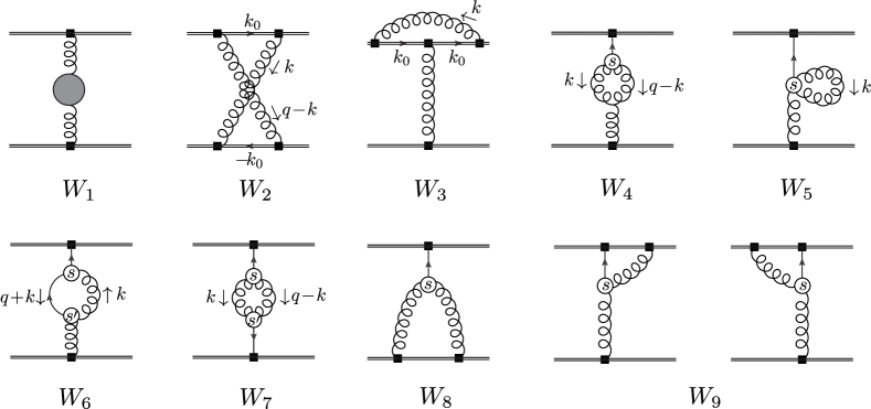
Figure 2: Feynman diagrams for the static potential at next-to-leading order in $\alpha_{s}$. The double lines represent temporal Wilson lines, curly lines are gluons, and solid lines are flow lines. The arrows on flow lines are in the direction of the greater flow time. Filled squares represent the flowed $B_{\mu}$ fields at flow time $t$, and open circles are flow vertices $X^{(n,0)}$. The blob in $W_{1}$ represents the gluon vacuum polarization.

In the computation of the NLO diagrams, we neglect the contributions that correspond to products of order-$\alpha_{s}$ contributions to $V(r)$, which arise from the perturbative expansion of $\langle W_{r\times T}\rangle\overset{T\to\infty}{=}e^{-V(r)T}$ beyond linear order. At order $\alpha_{s}^{2}$, the contribution to $V(r)$ can be extracted by writing the color factors as linear combinations of $C_{F}^{2}$ and $C_{F}C_{A}$, and discarding the terms proportional to $C_{F}^{2}$, because the $C_{F}^{2}$ terms correspond to the $[-V(r)T]^{2}/2$ term in the perturbative expansion of $e^{-V(r)T}$. Here, $C_{A}=N_{c}$.

We now discuss one by one the computation of the diagrams in figure 2. Diagram $W_{1}$ comes from the gluon vacuum polarization at one loop. In Feynman gauge, $W_{1}$ is given by

$$W_{1}=\frac{g^{4}C_{F}}{16\pi^{2}\bm{q}^{2}}e^{-2\bm{q}^{2}t}\left[\frac{31}{9}C_{A}-\frac{10}{9}n_{f}+\left(\frac{5}{3}C_{A}-\frac{2}{3}n_{f}\right)\left(\frac{1}{\epsilon_{\rm UV}}+\log(\mu^{2}/\bm{q}^{2})\right)\right],$$ (13)

where $n_{f}$ is the number of massless quark flavors. We use the label UV to indicate the ultraviolet origin of the $1/\epsilon$ pole.

Diagram $W_{2}$ is given by

$$W_{2} = \frac{1}{2}g^{4}C_{F}C_{A}\int\frac{d^{d}k}{(2\pi)^{d}}\frac{e^{-2t[k^{2}+(q-k)^{2}]}}{k^{2}(q-k)^{2}(k_{0}+i\varepsilon)^{2}}$$ (14)

$$= -\frac{1}{2}g^{4}C_{F}C_{A}\frac{e^{-2\bm{q}^{2}t}}{\bm{q}^{2+2\epsilon}}\frac{({\mu^{2}e^{\gamma_{\rm E}}})^{\epsilon}}{8\pi^{2}}\int_{0}^{\infty}dx\int_{0}^{\infty}dy\,\frac{\exp\left(\frac{4\bar{t}^{2}-xy}{4\bar{t}+x+y}\right)}{(x+y+4\bar{t})^{1-\epsilon}},$$

where we have used Schwinger parametrization, we have integrated over $k$ to obtain the parameter integral in the last line, and set $\bar{t}\equiv\bm{q}^{2}t$. The parameter integral is IR divergent for $\epsilon=0$, which can be seen from the behavior of the integrand at $x\to\infty$ or $y\to\infty$. We employ sector decomposition Hepp:1966eg ; Binoth:2000ps ; Binoth:2003ak ; Heinrich:2008si to compute the parameter integral, which provides a way to separate the divergent and finite contributions. The finite contribution is obtained in the form of a parameter integral that is finite at $\epsilon=0$, so that we can expand the integrand in powers of $\epsilon$. We change the integration variables according to $x=\bar{t}x_{1}/(1-x_{1})$ and $y=\bar{t}x_{2}/(1-x_{2})$, so that the region of integration is a unit square given by $0<x_{1}<1$ and $0<x_{2}<1$. The region of integration is then divided into the sectors $x_{1}<x_{2}$ and $x_{1}>x_{2}$; the contribution from each sector can again be expressed as an integral over a unit square by rescaling the integration variables. We obtain

$$W_{2}=g^{4}C_{F}C_{A}\frac{e^{-2\bm{q}^{2}t}}{16\pi^{2}\bm{q}^{2}}\left[2\left(\frac{1}{\epsilon_{\rm IR}}+\log(\mu^{2}/\bm{q}^{2})\right)+W_{2}^{F}(\bar{t})+O(\epsilon)\right],$$ (15)

where we use the label IR to indicate the infrared origin of the $1/\epsilon$ pole, and $W_{2}^{F}(\bar{t})$ is the finite piece given by

$$W_{2}^{F}(\bar{t})=2\left[e^{2\bar{t}}\left(\text{Ei}(-\bar{t})-2\,\text{Ei}(-2\bar{t})\right)-\text{Ei}(\bar{t})+2\log 2+2\log\bar{t}+2\gamma_{\rm E}\right].$$ (16)

The function $\text{Ei}(z)$ is the exponential integral defined by

$$\text{Ei}(x)=\int_{-x}^{\infty}\frac{e^{-t}}{t}dt.$$ (17)

Diagram $W_{3}$ can be computed in a similar way. We have

$$W_{3}=-g^{4}C_{F}C_{A}\frac{e^{-2\bm{q}^{2}t}}{\bm{q}^{2}}\int\frac{d^{d}k}{(2\pi)^{d}}\frac{1}{k^{2}(k_{0}+i\varepsilon)^{2}}e^{-2tk^{2}}.$$ (18)

We use Schwinger parametrization to combine the $k^{2}$ in the denominator and the exponent. We obtain

$$W_{3} = -g^{4}C_{F}C_{A}\frac{e^{-2\bm{q}^{2}t}}{\bm{q}^{2}}\int_{0}^{\infty}dx\int\frac{d^{d}k}{(2\pi)^{d}}\frac{1}{(k_{0}+i\varepsilon)^{2}}e^{-(x+2t)k^{2}}$$ (19)

$$= \frac{(\mu^{2}e^{\gamma_{\rm E}})^{\epsilon}}{8\pi^{2}}g^{4}C_{F}C_{A}\frac{e^{-2\bm{q}^{2}t}}{\bm{q}^{2}}\int_{0}^{\infty}\frac{dx}{(x+2t)^{1-\epsilon}}$$

$$= g^{4}C_{F}C_{A}\frac{e^{-2\bm{q}^{2}t}}{16\pi^{2}\bm{q}^{2}}\left[-2\left(\frac{1}{\epsilon_{\rm IR}}+\log(\mu^{2}/\bm{q}^{2})\right)+W_{3}^{F}(\bar{t})+O(\epsilon)\right],$$

where

$$W_{3}^{F}(\bar{t})=-2[\log(2\bar{t})+\gamma_{\rm E}].$$ (20)

The pole in $\epsilon$ comes from the divergence of the parameter integral at large $x$, which corresponds to the vanishing of $k^{2}$. Hence, the pole in $W_{3}$ is an IR pole. We note that the IR poles cancel in $W_{2}+W_{3}$, similarly to the QCD case Fischler:1977yf .

The computation of the UV-divergent diagrams $W_{4}$–$W_{6}$ can be done in a similar way. We have

$$W_{4} = \frac{2g^{4}C_{A}C_{F}}{\bm{q}^{2}}\int_{0}^{t}ds\,e^{-(2t-s)q^{2}}\int\frac{d^{d}k}{(2\pi)^{d}}e^{-s(k^{2}+(q-k)^{2})}\frac{2(d-2)k_{0}^{2}+q^{2}+2k^{2}}{k^{2}(q-k)^{2}},$$ (21)

$$W_{5} = -\frac{2(d-1)g^{4}C_{A}C_{F}}{\bm{q}^{2}}e^{-2\bm{q}^{2}t}\int_{0}^{t}ds\,\int\frac{d^{d}k}{(2\pi)^{d}}\frac{1}{k^{2}}e^{-2sk^{2}},$$ (22)

$$W_{6} = \frac{4g^{4}C_{A}C_{F}}{\bm{q}^{2}}e^{-2\bm{q}^{2}t}\int_{0}^{t}ds\int_{0}^{s}ds^{\prime}\int\frac{d^{d}k}{(2\pi)^{d}}e^{sq^{2}-(s-s^{\prime})(q+k)^{2}-(s+s^{\prime})k^{2}-s^{\prime}q^{2}}$$ (23)

$$\hskip 150.69397pt\times\frac{2(d-2)k_{0}^{2}+k^{2}+k\cdot q+2q^{2}}{k^{2}}.$$

We use again Schwinger parametrization to exponentiate the gluon propagator denominators. After integrating over $k$, we obtain expressions that are integrals over the Schwinger parameters and the flow times $s$ and $s^{\prime}$. These integrals can then be reexpressed as integrals over a unit hypercube, in a way similar to what we have done for the computation of $W_{2}$, and by rescaling the flow times $s$ and $s^{\prime}$. We then use sector decomposition to extract the UV poles of the parameter integrals and obtain the following expressions:

$$W_{4} = g^{4}C_{A}C_{F}\frac{e^{-2\bm{q}^{2}t}}{16\pi^{2}\bm{q}^{2}}\left[3\left(\frac{1}{\epsilon_{\rm UV}}+\log(\mu^{2}/\bm{q}^{2})\right)+W_{4}^{F}(\bar{t})+O(\epsilon)\right],$$ (24)

$$W_{5} = g^{4}C_{A}C_{F}\frac{e^{-2\bm{q}^{2}t}}{16\pi^{2}\bm{q}^{2}}\left[-3\left(\frac{1}{\epsilon_{\rm UV}}+\log(\mu^{2}/\bm{q}^{2})\right)+W_{5}^{F}(\bar{t})+O(\epsilon)\right],$$ (25)

$$W_{6} = g^{4}C_{A}C_{F}\frac{e^{-2\bm{q}^{2}t}}{16\pi^{2}\bm{q}^{2}}\left[2\left(\frac{1}{\epsilon_{\rm UV}}+\log(\mu^{2}/\bm{q}^{2})\right)+W_{6}^{F}(\bar{t})+O(\epsilon)\right],$$ (26)

where the terms $W_{4}^{F}(\bar{t})$, $W_{5}^{F}(\bar{t})$, and $W_{6}^{F}(\bar{t})$ can be written as integrals over a unit hypercube that are finite at $d=4$. The analytical expression for $W_{5}^{F}(\bar{t})$ is given by

$$W_{5}^{F}(\bar{t})=-1-3\gamma_{\rm E}-3\log(2\bar{t}).$$ (27)

We have not found analytical expressions for $W_{4}^{F}(\bar{t})$ and $W_{6}^{F}(\bar{t})$. We show $W_{4}^{F}(\bar{t})$ and $W_{6}^{F}(\bar{t})$ as integrals over a unit hypercube in appendix A. The UV poles of $W_{4}$ and $W_{5}+W_{6}$ agree with the results in ref. Luscher:2011bx .

The remaining diagrams $W_{7}$–$W_{9}$ yield

$$W_{7} = 2g^{4}C_{A}C_{F}\int_{0}^{t}ds\int_{0}^{t}ds^{\prime}\int\frac{d^{d}k}{(2\pi)^{d}}e^{-(s+s^{\prime})(k^{2}+(k-q)^{2})-(t-s-s^{\prime})q^{2}}\frac{(d-2)k_{0}^{2}+2k^{2}}{k^{2}(q-k)^{2}},\quad\quad$$ (28)

$$W_{8} = 2g^{4}C_{A}C_{F}\int_{0}^{t}ds\,e^{-(t-s)q^{2}}\int\frac{d^{d}k}{(2\pi)^{d}}e^{-s(k^{2}+(q-k)^{2})}\frac{e^{-k^{2}t}}{k^{2}}\frac{e^{-(q-k)^{2}t}}{(q-k)^{2}},$$ (29)

$$W_{9} = -2g^{4}C_{A}C_{F}\int\frac{d^{d}k}{(2\pi)^{d}}\int_{0}^{t}ds\,e^{-(t-s)(q-k)^{2}}e^{-s(k^{2}+q^{2})}\frac{e^{-q^{2}t}}{q^{2}}\frac{e^{-k^{2}t}}{k^{2}}.$$ (30)

Since these diagrams are finite, we can compute them at $d=4$. We again compute these diagrams by using Schwinger parametrization. After integrating over $k$, we obtain

$$W_{7} = g^{4}C_{A}C_{F}\frac{e^{-2\bm{q}^{2}t}}{16\pi^{2}\bm{q}^{2}}W_{7}^{F}(\bar{t})+O(\epsilon),$$ (31)

$$W_{8} = g^{4}C_{A}C_{F}\frac{e^{-2\bm{q}^{2}t}}{16\pi^{2}\bm{q}^{2}}W_{8}^{F}(\bar{t})+O(\epsilon),$$ (32)

$$W_{9} = g^{4}C_{A}C_{F}\frac{e^{-2\bm{q}^{2}t}}{16\pi^{2}\bm{q}^{2}}W_{9}^{F}(\bar{t})+O(\epsilon),$$ (33)

where $W_{7}^{F}(\bar{t})$, $W_{8}^{F}(\bar{t})$, and $W_{9}^{F}(\bar{t})$ are parameter integrals over a unit hypercube; explicit expressions can be found in appendix A. The expressions for $W_{8}^{F}$ and $W_{9}^{F}$ can be further simplified into

$$W_{8}^{F}(\bar{t}) = -2\left\{2e^{2\bar{t}}\text{Ei}\left(-2\bar{t}\right)+e^{\bar{t}}\left[\text{Ei}\left(-\frac{\bar{t}}{2}\right)-(e^{\bar{t}}+2)\text{Ei}\left(-\bar{t}\right)\right]+\text{Ei}\left(\frac{\bar{t}}{2}\right)-\text{Ei}\left(\bar{t}\right)\right\},\quad\quad$$ (34)

$$W_{9}^{F}(\bar{t}) = \frac{1}{\bar{t}}\left[-\sqrt{2\pi\bar{t}}\,\text{erfi}\left(\sqrt{\bar{t}/2}\right)+2e^{\bar{t}/2}-2\right],$$ (35)

where, $\text{erfi}(z)=-i\,\text{erf}(iz)$ is the imaginary error function, and

$$\text{erf}(z)=\frac{2}{\sqrt{\pi}}\int_{0}^{z}dt\,e^{-t^{2}}.$$ (36)

As a cross check of our results, we have also evaluated the diagrams $W_{2}$–$W_{9}$ by using different parameterizations of the Feynman integrals and evaluating them numerically, and found agreements in all cases. In the case of divergent diagrams, the use of different parameterizations leads to expressions of divergent and finite integrands that differ nontrivially from what we have obtained above, and so, the agreement in the sum of the divergent and finite contributions to each diagram serves as an independent check of our results.

3.3 Results in momentum space

The total one-loop correction to $-\tilde{V}(\bm{q};t)$ is given by

$$\sum_{n=1}^{9}W_{n}=\frac{4\pi\alpha_{s}C_{F}e^{-2\bm{q}^{2}t}}{\bm{q}^{2}}\frac{\alpha_{s}}{4\pi}\bigg{[}\beta_{0}\left(\frac{1}{\epsilon_{\rm UV}}+\log(\mu^{2}/\bm{q}^{2})\right)+a_{1}+C_{A}\,W_{\rm NLO}^{F}(\bar{t})+O(\epsilon)\bigg{]},$$ (37)

where $\displaystyle\beta_{0}=\frac{11}{3}C_{A}-\frac{2}{3}n_{f}$, and

$$a_{1} = \frac{31}{9}C_{A}-\frac{10}{9}n_{f},$$ (38)

$$W_{\rm NLO}^{F}(\bar{t}) = \sum_{n=2}^{9}W_{n}^{F}(\bar{t}).$$ (39)

The UV pole is subtracted by renormalization of the strong coupling. In the $\overline{\rm MS}$ scheme, we find

$$\tilde{V}(\bm{q};t) = -\frac{4\pi\alpha_{s}(\mu)C_{F}e^{-2\bm{q}^{2}t}}{\bm{q}^{2}}$$ (40)

$$\times\bigg{\{}1+\frac{\alpha_{s}(\mu)}{4\pi}\bigg{[}\beta_{0}\log(\mu^{2}/\bm{q}^{2})+a_{1}+C_{A}\,W_{\rm NLO}^{F}(\bar{t})\bigg{]}\bigg{\}}+O(\alpha_{s}^{3}),$$

where now $\alpha_{s}(\mu)$ is the strong coupling constant in the $\overline{\rm MS}$ scheme, and $\mu$ is the renormalization scale. The term $a_{1}$ is the finite piece of the one-loop correction to the static potential in regular QCD Fischler:1977yf , while $C_{A}\,W_{\rm NLO}^{F}(\bar{t})$ is the extra finite term that appears in gradient flow.

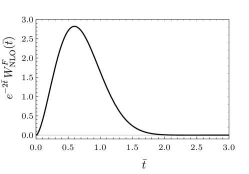
Figure 3: The finite correction term $e^{-2\bar{t}}W_{\rm NLO}^{F}(\bar{t})$ as a function of $\bar{t}=\bm{q}^{2}t$.

Since we have not obtained analytical results for some of the one-loop diagrams, we compute $W_{\rm NLO}^{F}(\bar{t})$ for arbitrary $\bar{t}$ by numerically evaluating the parameter integrals given in the appendix. As $\bar{t}$ increases, $W_{\rm NLO}^{F}(\bar{t})$ diverges like $e^{\bar{t}}/\bar{t}$. However, when multiplied by the factor $e^{-2\bm{q}^{2}t}=e^{-2\bar{t}}$, the extra finite term still decreases exponentially at large $\bar{t}$. We show the numerical results for $e^{-2\bar{t}}\,W_{\rm NLO}^{F}(\bar{t})$ in figure 3.

It is possible to show analytically that $W_{\rm NLO}^{F}(\bar{t})$ vanishes in the limit $\bar{t}\to 0$, so that we recover the QCD result as expected. From the analytical expressions, we have the following expansions at $\bar{t}=0$:

$$W_{2}^{F}(\bar{t}) = -4\bar{t}\left[-1+\gamma_{\rm E}+\log(4\bar{t})\right]+O(\bar{t}^{2}),$$ (41)

$$W_{8}^{F}(\bar{t}) = -2\bar{t}[-2+\gamma_{\rm E}+\log(8\bar{t})]+O(\bar{t}^{2}),$$ (42)

$$W_{9}^{F}(\bar{t}) = -1-\frac{\bar{t}}{12}+O(\bar{t}^{2}),$$ (43)

moreover we find the following expansions by computing the parameter integrals near $t=0$:

$$W_{4}^{F}(\bar{t}) = 3\log(2\bar{t})+3\gamma_{\rm E}+\frac{5}{2}+\bar{t}\left[-\frac{4}{3}\log(2\bar{t})-\frac{4}{3}\gamma_{\rm E}+\frac{31}{9}\right]+O(\bar{t}^{2}),$$ (44)

$$W_{6}^{F}(\bar{t}) = 2\log(2\bar{t})+2\gamma_{\rm E}-\frac{1}{2}+\frac{145}{36}\bar{t}+O(\bar{t}^{2}),$$ (45)

$$W_{7}^{F}(\bar{t}) = 5\bar{t}\log 2+O(\bar{t}^{2}).$$ (46)

The $\bar{t}\log\bar{t}$ term in $W_{4}^{F}(\bar{t})$ arises from divergences in the parameter integral when the integrand is expanded in powers of $\bar{t}$; the coefficient of the $\bar{t}\log\bar{t}$ term can be computed by isolating the divergent regions in the limit $\bar{t}\to 0$. By using the above expansions and the exact analytical expressions of $W_{3}^{F}(\bar{t})$ and $W_{5}^{F}(\bar{t})$, we obtain

$$W_{\rm NLO}^{F}(\bar{t})=\bar{t}\left(-\frac{22\gamma_{\rm E}}{3}+\frac{277}{18}-\frac{31\log 2}{3}-\frac{22}{3}\log\bar{t}\right)+O(\bar{t}^{2}).$$ (47)

Since the $\bar{t}\log\bar{t}$ terms do not cancel in $W_{\rm NLO}^{F}(\bar{t})$, we find that the $t$-dependent one-loop finite term is not analytical at $t=0$, even though $W_{\rm NLO}^{F}(\bar{t})$ vanishes in the limit $t\to 0$ as expected. The order-$\bar{t}$ term in eq. (47) will be crucial in obtaining the behavior of the position-space static force in the limit $t\to 0$ in the next section.

3.4 Results in position space

We now turn to position space to obtain

$$F(r;t)=\frac{\partial}{\partial r}\int\frac{d^{3}\bm{q}}{(2\pi)^{3}}\tilde{V}(\bm{q};t)e^{i\bm{q}\cdot\bm{r}}=\frac{1}{r^{2}}\int_{0}^{\infty}d|\bm{q}|\bm{q}^{2}\frac{|\bm{q}|r\cos(|\bm{q}|r)-\sin(|\bm{q}|r)}{2\pi^{2}|\bm{q}|}\tilde{V}(\bm{q};t).$$ (48)

By using the fact that $r^{2}F(r;t)$ is dimensionless, we define the following dimensionless quantities

$${\cal F}_{0}(r;t) = -\int_{0}^{\infty}d|\bm{q}|\bm{q}^{2}\frac{|\bm{q}|r\cos(|\bm{q}|r)-\sin(|\bm{q}|r)}{2\pi^{2}|\bm{q}|}\frac{4\pi e^{-2\bm{q}^{2}t}}{\bm{q}^{2}},$$ (49)

$${\cal F}_{\rm NLO}^{L}(r;t;\mu) = -\int_{0}^{\infty}d|\bm{q}|\bm{q}^{2}\frac{|\bm{q}|r\cos(|\bm{q}|r)-\sin(|\bm{q}|r)}{2\pi^{2}|\bm{q}|}\frac{4\pi e^{-2\bm{q}^{2}t}}{\bm{q}^{2}}\log(\mu^{2}/\bm{q}^{2}),$$ (50)

$${\cal F}_{\rm NLO}^{F}(r;t) = -\int_{0}^{\infty}d|\bm{q}|\bm{q}^{2}\frac{|\bm{q}|r\cos(|\bm{q}|r)-\sin(|\bm{q}|r)}{2\pi^{2}|\bm{q}|}\frac{4\pi e^{-2\bm{q}^{2}t}}{\bm{q}^{2}}W_{\rm NLO}^{F}(\bar{t}=\bm{q}^{2}t),$$ (51)

so that

$$F(r;t) = \frac{\alpha_{s}(\mu)C_{F}}{r^{2}}\bigg{[}\left(1+\frac{\alpha_{s}}{4\pi}a_{1}\right){\cal F}_{0}(r;t)$$ (52)

$$\hskip 51.6665pt+\frac{\alpha_{s}}{4\pi}\beta_{0}{\cal F}_{\rm NLO}^{L}(r;t;\mu)+\frac{\alpha_{s}C_{A}}{4\pi}{\cal F}_{\rm NLO}^{F}(r;t)\bigg{]}+O(\alpha_{s}^{3}).$$

The integrands for ${\cal F}_{0}(r;t)$ and ${\cal F}_{\rm NLO}^{L}(r;t;\mu)$ involve the factor $e^{-2\bm{q}^{2}t}$ that makes the integrands decrease exponentially at large $|\bm{q}|$, so that the Fourier transforms converge rapidly. In the case of ${\cal F}_{\rm NLO}^{F}(r;t)$, the convergence is slower, because $W_{\rm NLO}^{F}(\bar{t})$ diverges exponentially at large $\bar{t}$. However, since $e^{-2\bm{q}^{2}t}W_{\rm NLO}^{F}(\bar{t}=\bm{q}^{2}t)$ still decreases exponentially at large $|\bm{q}|$, the integral in ${\cal F}_{\rm NLO}^{F}(r;t)$ still converges rapidly.

The quantities ${\cal F}_{0}(r;t)$ and ${\cal F}_{\rm NLO}^{L}(r;t;\mu)$ can be computed analytically:

$${\cal F}_{0}(r;t) = \text{erf}\left(\frac{r}{\sqrt{8t}}\right)-\frac{r}{\sqrt{2\pi t}}\exp\left(-\frac{r^{2}}{8t}\right),$$ (53)

$${\cal F}_{\rm NLO}^{L}(r;t;\mu) = \log(\mu^{2}r^{2}){\cal F}_{0}(r;t)+\log\left(\frac{8t}{r^{2}}e^{\gamma_{\rm E}}\right){\cal F}_{0}(r;t)$$ (54)

$$-\frac{r}{\sqrt{2\pi t}}\left[e^{-\frac{r^{2}}{8t}}M^{(1,0,0)}\left(0,\frac{1}{2},\frac{r^{2}}{8t}\right)+M^{(1,0,0)}\left(\frac{1}{2},\frac{3}{2},-\frac{r^{2}}{8t}\right)\right],$$

where $M(a,b,z)$ is the confluent hypergeometric function defined by

$$M(a,b,z)=\sum_{k=0}^{\infty}\frac{(a)_{k}}{(b)_{k}}\frac{z^{k}}{k!},$$ (55)

with $(x)_{k}=\Gamma(x+k)/\Gamma(x)$, and

$$M^{(1,0,0)}(a,b,z)=\frac{\partial}{\partial a}M(a,b,z).$$ (56)

We note that ${\cal F}_{0}(r;t)$ is a function of $r/\sqrt{t}$ only. This function vanishes at $r=0$, and $\displaystyle\lim_{t\to 0}{\cal F}_{0}(r;t)=1$. We show ${\cal F}_{0}(r;t)$ as a function of $r/\sqrt{t}$ in figure 4.

Figure 4: The factor ${\cal F}_{0}(r;t)$ as a function of $r/\sqrt{t}$.

Combining the corrections $\log(\mu^{2}r^{2}){\cal F}_{0}(r;t)$ and $\log(8t/r^{2}){\cal F}_{0}(r;t)$ in ${\cal F}_{\rm NLO}^{L}(r;t;\mu)$ may suggest that the logarithmic corrections in ${\cal F}_{\rm NLO}^{L}$ will be suppressed if we set $\mu=1/\sqrt{8t}$. This is indeed the case for $r^{2}/t\ll 1$, since in this limit the hypergeometric functions in ${\cal F}_{\rm NLO}^{L}(r;t;\mu)$ are analytic. On the other hand, the contributions to ${\cal F}_{\rm NLO}^{L}(r;t;\mu)$ other than $\log(\mu^{2}r^{2}){\cal F}_{0}(r;t)$ assume the constant value $2(\gamma_{\rm E}-1)$ in the opposite limit $r^{2}/t\to\infty$. Hence, the relevant scale for the one-loop correction is $\mu=1/r$ for $r^{2}/t\gg 1$, while it is $\mu=1/\sqrt{8t}$ for $r^{2}/t\ll 1$. We find that the scale choice $\mu=(r^{2}+8t)^{-1/2}$ makes the logarithmic correction factor ${\cal F}_{\rm NLO}^{L}(r;t;\mu)/{\cal F}_{0}(r;t)$ of order 1 for all values of $r/\sqrt{t}$, in contrast to the choices $\mu=1/r$ or $\mu=1/\sqrt{8t}$. This is shown in figure 5. Furthermore we have that ${\cal F}_{\rm NLO}^{L}(r;t;\mu)$ approaches the limit $t\to 0$ linearly in $t$, in the form

$${\cal F}_{\rm NLO}^{L}(r;t;\mu)\approx\log(\mu^{2}r^{2})+2(\gamma_{\rm E}-1)-12\frac{t}{r^{2}},$$ (57)

which can be obtained from the asymptotic expansion of $M(a,b,z)$ for large $z$ (see, for example, ref. NIST:DLMF ).

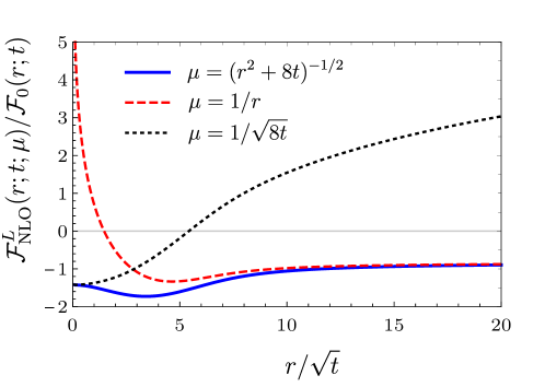
Figure 5: The logarithmic correction factor ${\cal F}_{\rm NLO}^{L}(r;t;\mu)/{\cal F}_{0}(r;t)$ for $\mu=(r^{2}+8t)^{-1/2}$, $\mu=1/r$, and $\mu=1/\sqrt{8t}$ shown as a function of $r/\sqrt{t}$.

Now we discuss the finite correction term ${\cal F}_{\rm NLO}^{F}(r;t)$. Since ${\cal F}_{\rm NLO}^{F}(r;t)$ is dimensionless, it is a function of $\xi=r/\sqrt{t}$ only, and we can rewrite ${\cal F}_{\rm NLO}^{F}(r;t)$ as

$${\cal F}_{\rm NLO}^{F}(r;t)=-\frac{2}{\pi}\int_{0}^{\infty}dx\left[\xi\cos(\xi x)-\frac{\sin(\xi x)}{x}\right]e^{-2x^{2}}W_{\rm NLO}^{F}(\bar{t}=x^{2}).$$ (58)

Because we compute $W_{\rm NLO}^{F}(\bar{t})$ numerically from the finite parameter integrals, also ${\cal F}_{\rm NLO}^{F}(r;t)$ is only known numerically for a given value of $\xi=r/\sqrt{t}$. We show ${\cal F}_{\rm NLO}^{F}(r;t)$ as a function of $\xi$ in figure 6. A function that approximates ${\cal F}_{\rm NLO}^{F}(r;t)$ better than 1% in the region $1<\xi<10$ and better than 2% in the region $\xi>10$ is

$$\sum_{n=1}^{10}\frac{c_{n}}{n!}\left(\frac{\xi}{1+\xi/C_{a}}\right)^{n}e^{-\xi}+\frac{44-C_{b}}{C_{a}+\xi^{2}}+\frac{C_{b}\xi^{2}}{\xi^{4}+C_{c}},$$ (59)

with $C_{a}=109.358$, $C_{b}=43.8438$, $C_{c}=404.790$, and $c_{n}$ listed in table 1. The function (59) does not reproduce ${\cal F}_{\rm NLO}^{F}(r;t)$ for $\xi<1$.

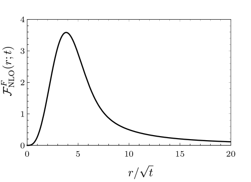
Figure 6: The finite one-loop correction ${\cal F}_{\rm NLO}^{F}(r;t)$ as a function of $r/\sqrt{t}$.

$c_{1}$	$-0.0501648$
$c_{2}$	$0.526758$
$c_{3}$	$-5.55177$
$c_{4}$	$45.8753$
$c_{5}$	$-147.8$
$c_{6}$	$463.906$
$c_{7}$	$-851.741$
$c_{8}$	$884.315$
$c_{9}$	$-499.105$
$c_{10}$	$121.773$

Table 1: Numerical values of the coefficients $c_{n}$ appearing in eq. (59) that make that function reproduce ${\cal F}_{\rm NLO}^{F}(r;t)$ for $1<r/\sqrt{t}<10$ better than 1%, and for $r/\sqrt{t}>10$ better than 2%.

For small values of $\xi$, we may expand the terms in the square brackets in eq. (58) as series in $\xi$ and compute the coefficients numerically to find

$${\cal F}_{\rm NLO}^{F}(r;t)=0.304930\,\xi^{3}-0.0332202\,\xi^{5}+0.00181358\,\xi^{7}+O(\xi^{9}).$$ (60)

The truncated series agrees with the numerical calculation of ${\cal F}_{\rm NLO}^{F}(r;t)$ for $\xi<0.5$ by better than $10^{-4}$, and for $0.5<\xi<1.0$ by better than $5\times 10^{-4}$.

For large values of $\xi$ (small $t$, fixed $r$), we derive the asymptotic behavior of ${\cal F}_{\rm NLO}^{F}(r;t)$ based on the behavior of $W_{\rm NLO}^{F}(\bar{t})$ at small $\bar{t}$ and the Riemann–Lebesgue lemma. We first rewrite ${\cal F}_{\rm NLO}^{F}(r;t)$ as

$${\cal F}_{\rm NLO}^{F}(r;t)=-\frac{2}{\pi}\int_{0}^{\infty}dx\left[\xi\cos(\xi x)f(x)-\sin(\xi x)g(x)\right],$$ (61)

where $f(x)=e^{-2x^{2}}W_{\rm NLO}^{F}(\bar{t}=x^{2})$, and $g(x)=f(x)/x$. We note that $f(x)\sim x^{2}\log(x/C)$ and $g(x)\sim x\log(x/C)$ for small $x$, where $C$ is a constant, while they both vanish exponentially at large $x$. We first consider the cosine term. By integrating by parts, we obtain

$$\xi\int_{0}^{\infty}dx\,\cos(\xi x)f(x)=-\int_{0}^{\infty}dx\sin(\xi x)f^{\prime}(x)=-\frac{1}{\xi}\int_{0}^{\infty}dx\cos(\xi x)f^{\prime\prime}(x).$$ (62)

In the first and second equalities, we used the fact that both $f(x)$ and $f^{\prime}(x)$ vanish at $x=0$ and $x=\infty$, so that the boundary terms vanish. From the Riemann–Lebesgue lemma, we see that the integral $\displaystyle\int_{0}^{\infty}dx\cos(\xi x)f^{\prime\prime}(x)$ vanishes in the limit $\xi\to\infty$, because $\displaystyle\int_{0}^{\infty}dx|f^{\prime\prime}(x)|$ is finite. We use integration by parts again to obtain

$$\xi\int_{0}^{\infty}dx\,\cos(\xi x)f(x)=-\frac{1}{\xi^{2}}\sin(\xi x)f^{\prime\prime}(x)\Big{|}_{x=0}^{\infty}+\frac{1}{\xi^{2}}\int_{0}^{\infty}dx\,\sin(\xi x)f^{\prime\prime\prime}(x).$$ (63)

Since $f^{\prime\prime}(x)$ diverges logarithmically and $\sin(\xi x)$ vanishes linearly at $x=0$, the boundary terms vanish. The Riemann–Lebesgue lemma does not apply to the last term, because $f^{\prime\prime\prime}(x)$ diverges like $1/x$. However, if we split the region of integration as

$$\xi\int_{0}^{\infty}dx\,\cos(\xi x)f(x)=\frac{1}{\xi^{2}}\left[\int_{0}^{a}dx\,\sin(\xi x)f^{\prime\prime\prime}(x)+\int_{a}^{\infty}dx\,\sin(\xi x)f^{\prime\prime\prime}(x)\right],$$ (64)

where $a$ is a positive constant, the second term in the square brackets vanishes in the limit $\xi\to\infty$, because $\displaystyle\int_{a}^{\infty}dx|f^{\prime\prime\prime}(x)|$ is finite. In the limit $\xi\to\infty$, we can see that the first term in the square brackets converges to a finite value by approximating $W_{\rm NLO}^{F}(\bar{t})$ by eq. (47). We obtain from the Dirichlet integral

$$\lim_{\xi\to\infty}\int_{0}^{a}dx\,\sin(\xi x)f^{\prime\prime\prime}(x)\approx 2\pi c_{L},$$ (65)

where $c_{L}=-22/3$ is the coefficient of $\bar{t}\log\bar{t}$ in eq. (47). Similarly, by using integration by parts we can rewrite the sine term of eq. (61) as

$$-\int_{0}^{\infty}dx\,\sin(\xi x)g(x)=\frac{1}{\xi^{2}}\left[\int_{0}^{a}dx\,\sin(\xi x)g^{\prime\prime}(x)+\int_{a}^{\infty}dx\,\sin(\xi x)g^{\prime\prime}(x)\right],$$ (66)

where the second term in the square brackets vanishes in the limit $\xi\to\infty$, and

$$\lim_{\xi\to\infty}\int_{0}^{a}dx\,\sin(\xi x)g^{\prime\prime}(x)\approx\pi c_{L}.$$ (67)

From these results we obtain the following asymptotic behavior for large $\xi$ given by

$${\cal F}_{\rm NLO}^{F}(r;t)\approx-\frac{6c_{L}}{\xi^{2}}.$$ (68)

This shows that ${\cal F}_{\rm NLO}^{F}(r;t)$ for a given $r$ vanishes in the limit $t\to 0$ linearly as $-6c_{L}t/r^{2}$. We recall that the $t\to 0$ limit is the relevant limit, the one that reduces the gradient flow to QCD.

We now show the numerical results for the static force in gradient flow, $r^{2}F(r;t)$, at NLO in $\alpha_{s}$. We compute $\alpha_{s}$ in the $\overline{\rm MS}$ scheme at the scale $\mu=(r^{2}+8t)^{-1/2}$ by using RunDec Chetyrkin:2000yt at four loops, and set $n_{f}=4$. At tree level, $r^{2}F(r;t=0)$ equals $\alpha_{s}C_{F}$, so that it increases with $r$, due to the evolution of $\alpha_{s}(\mu=1/r)$.

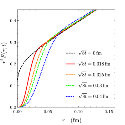
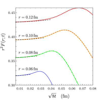
Figure 7: Left panel: numerical results for $r^{2}F(r;t)$ for fixed values of $\sqrt{8t}$ as functions of $r$. Right panel: numerical results for $r^{2}F(r;t)$ for fixed values of $r$ as functions of $\sqrt{8t}$; the black dashed lines are approximate results based on eq. (69), which is valid at small flow time. We have set $\mu=(r^{2}+8t)^{-1/2}$ and $n_{f}=4$.

In the left panel of figure 7, we show $r^{2}F(r;t)$ as a function of $r$ for several fixed values of $\sqrt{8t}$. We can see that $r^{2}F(r;t)$ vanishes for $r\to 0$, while we recover the QCD result $r^{2}F(r;t=0)$ (black dashed line) for $r\gg\sqrt{8t}$. We observe that $r^{2}F(r;t)$ slightly overshoots the QCD result before converging to the $t\to 0$ limit, which comes from the positive correction due to ${\cal F}_{\rm NLO}^{F}(r;t)$ being larger than the negative correction due to ${\cal F}_{\rm NLO}^{L}(r;t;\mu)$.

In the right panel of figure 7, we show $r^{2}F(r;t)$ as a function of $t$ for several fixed values of $r$. For large $t$ ($\sqrt{8t}\gtrsim r$), $r^{2}F(r;t)$ is below the QCD result (given by the $t\to 0$ limit). As $t$ decreases, $r^{2}F(r;t)$ slightly overshoots the QCD result before converging to it. Again, this overshoot comes mainly from the positive correction due to ${\cal F}_{\rm NLO}^{F}$.

By using the asymptotic expansions of ${\cal F}_{\rm NLO}^{L}(r;t;\mu)$ and ${\cal F}_{\rm NLO}^{F}(r;t)$ for small $t$, we can derive the behavior of $r^{2}F(r;t)$ near $t=0$ as

$$r^{2}F(r;t)\approx r^{2}F(r;t=0)+\frac{\alpha_{s}^{2}C_{F}}{4\pi}\left[-12\beta_{0}-6C_{A}c_{L}\right]\frac{t}{r^{2}},$$ (69)

where $c_{L}=-22/3$ and $F(r;t=0)$ is the usual QCD result for the static force

$$F(r;t=0)=\frac{\alpha_{s}(\mu)C_{F}}{r^{2}}\left\{1+\frac{\alpha_{s}}{4\pi}\left[a_{1}+2\beta_{0}\log(\mu re^{\gamma_{\rm E}-1})\right]\right\}+O(\alpha_{s}^{3}).$$ (70)

For any positive $n_{f}$, the coefficient of the $t/r^{2}$ term is positive, and grows linearly with increasing $n_{f}$: specifically it is $\left[-12\beta_{0}-6C_{A}c_{L}\right]=8n_{f}$. Surprisingly the coefficient of the $t/r^{2}$ term vanishes at NLO in the pure SU(3) gauge theory ($n_{f}=0$). We compare the exact NLO result for $r^{2}F(r;t)$ at small $t$ with the expression given in eq. (69), in the right panel of figure 7. The function (69), which is quadratic in $\sqrt{8t}$ for $n_{f}=4$, is represented by the dashed black curve. The exact result approaches smoothly the approximate one at small flow time.

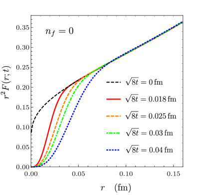
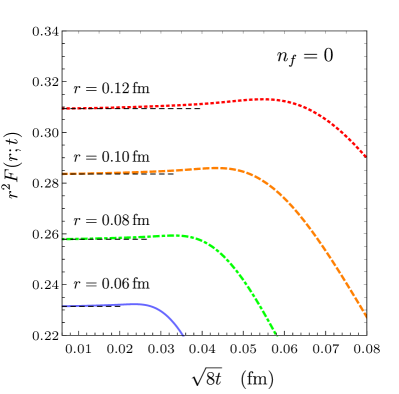
Figure 8: Left panel: numerical results for $r^{2}F(r;t)$ in the pure SU(3) gauge theory ($n_{f}=0$) for fixed values of $\sqrt{8t}$ as functions of $r$. Right panel: numerical results for $r^{2}F(r;t)$ in the pure SU(3) gauge theory ($n_{f}=0$) for fixed values of $r$ as functions of $\sqrt{8t}$; the black dashed lines are the QCD results for $r^{2}F(r;t=0)$. We have set $\mu=(r^{2}+8t)^{-1/2}$.

We also show $r^{2}F(r;t)$ in the pure SU(3) gauge theory ($n_{f}=0$) in figure 8 as a function of $r$ for fixed values of $\sqrt{8t}$, and as a function of $\sqrt{8t}$ for fixed values of $r$. We have computed $\alpha_{s}$ in the pure SU(3) gauge theory by using RunDec Chetyrkin:2000yt at four loops, based on the value $r_{0}\Lambda_{\rm QCD}=0.637^{+0.032}_{-0.030}$ in ref. Brambilla:2010pp , with $r_{0}=0.5$ fm Necco:2001xg . Due to the vanishing of the term linear in $t$ in eq. (69), the expression in eq. (69) is equal to the QCD result $r^{2}F(r;t=0)$, which we show in the right panel of figure 8 as horizontal black dashed lines.

4 Summary and discussion

In this work, we have computed the QCD static force and potential in gradient flow to next-to-leading order (NLO) accuracy in the strong coupling. The details of the NLO calculation have been given in section 3.2. The results in momentum space have been summarized in section 3.3, and the position-space results for the force have been given in section 3.4. As we have anticipated in the introduction, the gradient flow makes the Fourier transform of the static force in momentum space better converging, because the nonzero flow time $t$ introduces an exponentially decreasing factor in the integrand. Thus, we expect that the use of gradient flow may as well improve the convergence towards the continuum limit of the lattice QCD calculation of the static force done at finite flow time. This is supported by the preliminary results in ref. Leino:2021-157/21 .

Once the continuum limit of the lattice calculation of the force at finite flow time has been reached, the position-space results presented in section 3.4 may be useful for extrapolating to zero flow time, i.e. to QCD. We have shown explicitly that, indeed, both momentum and position-space NLO results reduce to the usual QCD result in the $t\to 0$ limit. We have also derived the NLO behavior of the static force in gradient flow near $t=0$, which is shown in eq. (69). The linear correction in $t$ vanishes in the pure SU(3) gauge theory, while it is positive for any positive number of massless quark flavors.

The NLO correction to the static force involves the length scale $\sqrt{8t}$, which often appears in loop-level calculations in gradient flow. Unlike the case of local operator matrix elements, an optimal choice of the renormalization scale $\mu$ is given by a combination of $1/r$ and $1/\sqrt{8t}$, rather than just the scale $1/\sqrt{8t}$. This happens because the static force depends only on the scale $1/r$ at $t=0$.

The fact that the static force in gradient flow involves two scales $1/r$ and $1/\sqrt{8t}$ brings in some complications in the investigation of its behavior near $t=0$. While the $t\to 0$ limit exists, since the static force is finite without renormalization of the gluon field, the NLO correction is not analytic at $t=0$, so that we cannot expand in powers of $t$ in a straightforward manner. If there was only one scale $1/\sqrt{8t}$, the nonanalyticity in $t$ could be read off from the $\log\mu$ terms in the NLO correction, which, in turn, are determined by the UV divergences. However, because of the two scales, the NLO correction involves complicated functions of the dimensionless ratio of the two scales, which happen to be nonanalytic at $t=0$. As a result, the derivation of the behavior of the static force near $t=0$ and beyond the $t\to 0$ limit in eq. (69) required a careful examination of the asymptotic expansion of the functions appearing in the NLO correction.

We expect this work to be of help in lattice QCD studies of the static force: if gradient flow provides a better convergence of direct lattice calculations of the force towards the continuum limit, the perturbative calculation done here adds a better controlled zero flow time limit. Similar analyses could be extended to a vast range of nonperturbative quarkonium observables in the factorization framework provided by nonrelativistic effective field theories Brambilla:2004jw . For instance, one could study in gradient flow the quarkonium potential at higher orders in $1/m$ Eichten:1979pu ; Barchielli:1988zp ; Bali:1997am ; Brambilla:2000gk ; Pineda:2000sz ; Brambilla:2003mu ; Koma:2006si ; Koma:2006fw ; Koma:2010zza , where $m$ is the heavy quark mass, static hybrid potentials Juge:2002br ; Capitani:2018rox ; Schlosser:2021wnr , hybrid potentials at higher orders in $1/m$ Oncala:2017hop ; Brambilla:2018pyn ; Brambilla:2019jfi , gluonic correlators entering the expressions of quarkonium inclusive widths and cross sections Brambilla:2001xy ; Brambilla:2002nu ; Brambilla:2020xod ; Brambilla:2020ojz ; Brambilla:2021abf .

Appendix A Finite parameter integrals at one loop

In this appendix, we show the expressions for the finite parameter integrals $W_{2}^{F}(\bar{t})$, $W_{4}^{F}(\bar{t})$, $W_{6}^{F}(\bar{t})$, $W_{7}^{F}(\bar{t})$, $W_{8}^{F}(\bar{t})$, and $W_{9}^{F}(\bar{t})$ that appear in the finite parts of the one-loop corrections to the static potential in gradient flow, see section 3.2. We express them as integrals over unit hypercubes of dimensions of up to 4. We also show the parameter integrals for $W_{2}^{F}(\bar{t})$, $W_{8}^{F}(\bar{t})$, and $W_{9}^{F}(\bar{t})$, even though we have computed them analytically in terms of exponential integrals and error functions, because the parameter integrals may be useful in some numerical analyses. We write $W_{4}^{F}(\bar{t})$, $W_{6}^{F}(\bar{t})$ and $W_{9}^{F}(\bar{t})$ as sums of analytic functions of $\bar{t}$ and parameter integrals that vanish at $\bar{t}=0$, so that the $\bar{t}\to 0$ limit can be easily identified. The expressions read:

$$W_{2}^{F}(\bar{t}) = -2\int_{0}^{1}dx_{1}dx_{2}\Bigg{[}\frac{\bar{t}x_{2}\exp\left(\frac{\left(3x_{1}x_{2}^{2}-4\left(x_{1}+1\right)x_{2}+4\right)\bar{t}}{2x_{1}x_{2}^{2}-3\left(x_{1}+1\right)x_{2}+4}\right)}{(x_{2}-1)\left(x_{1}x_{2}-1\right)\left(2x_{1}x_{2}^{2}-3\left(x_{1}+1\right)x_{2}+4\right)}$$ (71)

$$\hskip 86.11084pt+\frac{\bar{t}e^{\frac{x_{1}\bar{t}}{x_{1}-1}}}{(x_{2}-1)\left(x_{1}-1\right){}^{2}}-\log\bar{t}-\gamma_{\rm E}\Bigg{]},$$

$$W_{4}^{F}(\bar{t}) = 3\log(2\bar{t})+3\gamma_{\rm E}+\frac{5}{2}$$ (72)

$$+\frac{1}{2}\int_{0}^{1}dx_{1}dx_{2}dx_{3}\Bigg{[}\frac{8\exp\left(\frac{x_{2}\left(x_{1}x_{2}-1\right)\bar{t}}{x_{1}\left(2x_{2}-1\right)-2}\right)}{x_{2}\left(-2x_{2}x_{1}+x_{1}+2\right){}^{2}}+\frac{8e^{\frac{x_{1}^{2}\left(x_{2}-1\right)x_{2}\bar{t}}{2x_{1}\left(x_{2}-1\right)-1}}}{x_{2}\left(1-2x_{1}\left(x_{2}-1\right)\right){}^{2}}$$

$$+\frac{16x_{2}\left(x_{3}-1\right)\left(x_{2}x_{3}-1\right)\exp\left(\frac{x_{2}x_{3}\left(x_{1}^{2}x_{2}\left(x_{3}-1\right)\left(x_{2}x_{3}-1\right)-1\right)\bar{t}}{2x_{1}\left(x_{3}-1\right)x_{3}x_{2}^{2}-2x_{1}\left(x_{3}-1\right)x_{2}-2x_{3}x_{2}+x_{2}+1}\right)}{x_{3}\left(2x_{1}\left(x_{3}-1\right)x_{3}x_{2}^{2}-2x_{1}\left(x_{3}-1\right)x_{2}-2x_{3}x_{2}+x_{2}+1\right){}^{3}}$$

$$+\frac{16x_{2}\left(x_{1}x_{2}x_{3}-1\right)\left(x_{2}x_{3}-1\right)\exp\left(\frac{x_{3}\left(-x_{2}x_{3}+x_{1}x_{2}\left(x_{2}\left(x_{3}^{2}-1\right)-x_{3}\right)+1\right)\bar{t}}{2x_{1}\left(x_{3}-1\right)x_{3}x_{2}^{2}-\left(x_{1}+1\right)\left(2x_{3}-1\right)x_{2}+2}\right)}{x_{3}\left(2x_{1}\left(x_{3}-1\right)x_{3}x_{2}^{2}-\left(x_{1}+1\right)\left(2x_{3}-1\right)x_{2}+2\right){}^{3}}$$

$$+\frac{16x_{2}\left(x_{3}-1\right)\left(x_{1}x_{2}x_{3}-1\right)\exp\left(\frac{x_{2}x_{3}\left(-x_{3}x_{2}+x_{2}+x_{1}\left(x_{2}^{2}\left(x_{3}-1\right)x_{3}-1\right)\right)\bar{t}}{2x_{1}\left(x_{3}-1\right)x_{3}x_{2}^{2}+\left(-2x_{3}x_{1}+x_{1}-2x_{3}+2\right)x_{2}+1}\right)}{x_{3}\left(2x_{1}\left(x_{3}-1\right)x_{3}x_{2}^{2}+\left(-2x_{3}x_{1}+x_{1}-2x_{3}+2\right)x_{2}+1\right){}^{3}}$$

$$-\frac{16x_{2}}{x_{3}\left(x_{1}x_{2}+x_{2}+2\right){}^{3}}-\frac{16x_{2}}{x_{3}\left(2x_{1}x_{2}+x_{2}+1\right){}^{3}}-\frac{16x_{2}}{x_{3}\left(\left(x_{1}+2\right)x_{2}+1\right){}^{3}}$$

$$+\frac{4\bar{t}\exp\left(\frac{\left(\left(x_{1}-1\right)\left(x_{2}-1\right)x_{3}^{2}-x_{1}x_{2}\right)\bar{t}}{-2x_{2}x_{1}+x_{1}+x_{2}+2\left(x_{1}-1\right)\left(x_{2}-1\right)x_{3}}\right)}{\left(-2x_{2}x_{1}+x_{1}+x_{2}+2\left(x_{1}-1\right)\left(x_{2}-1\right)x_{3}\right){}^{2}}$$

$$-\frac{8}{x_{2}\left(2x_{1}+1\right){}^{2}}-\frac{8}{x_{2}\left(x_{1}+2\right){}^{2}}-2\log\left(\frac{81}{2}\right)\Bigg{]},$$

$$W_{6}^{F}(\bar{t}) = 2\log(2\bar{t})+2\gamma_{\rm E}-\frac{1}{2}$$ (73)

$$+\frac{1}{6}\int_{0}^{1}dx_{1}dx_{2}dx_{3}\Bigg{[}\frac{48\left(x_{2}-1\right)x_{1}\exp\left(\frac{x_{1}^{2}\left(x_{2}-1\right)x_{2}\left(x_{3}-1\right){}^{2}\bar{t}}{2x_{1}\left(x_{2}-1\right)-1}\right)}{x_{2}\left(2x_{1}\left(x_{2}-1\right)-1\right){}^{3}}$$

$$+\frac{48\left(x_{1}x_{2}-1\right)\exp\left(\frac{x_{2}\left(x_{1}x_{2}-1\right)\left(x_{3}-1\right){}^{2}\bar{t}}{x_{1}\left(2x_{2}-1\right)-2}\right)}{x_{2}\left(x_{1}\left(2x_{2}-1\right)-2\right){}^{3}}$$

$$+\frac{24x_{2}\left(\left(x_{1}-1\right)x_{2}\left(x_{3}+3\right)-2x_{1}\right)\bar{t}\exp\left(\frac{\left(x_{1}-1\right)x_{2}^{2}\left(x_{3}-1\right){}^{2}\bar{t}}{2\left(x_{1}-1\right)x_{2}-x_{1}}\right)}{\left(2\left(x_{1}-1\right)x_{2}-x_{1}\right){}^{3}}$$

$$+\frac{6\left(e^{\frac{1}{2}\left(x_{1}-1\right){}^{2}x_{2}\bar{t}}-1\right)}{x_{2}}-\frac{48x_{1}}{x_{2}\left(2x_{1}+1\right){}^{3}}-\frac{48}{x_{2}\left(x_{1}+2\right){}^{3}}+4-6\log 3\Bigg{]},$$

$$W_{7}^{F}(\bar{t}) = 4\int_{0}^{1}dx_{1}dx_{2}dx_{3}dx_{4}\Bigg{[}\frac{\bar{t}\exp\left(\frac{\bar{t}\left(x_{1}-1\right)\left(x_{2}+x_{3}\right){}^{2}}{-x_{1}+2\left(x_{1}-1\right)x_{2}+2\left(x_{1}-1\right)x_{3}}\right)}{\left(x_{1}-2\left(x_{1}-1\right)x_{2}-2\left(x_{1}-1\right)x_{3}\right){}^{2}}$$

$$+\frac{\bar{t}\left(x_{1}-1\right)\left(x_{2}-1\right)\exp\left(\frac{\bar{t}\left(\left(x_{1}-1\right)\left(x_{2}-1\right)x_{3}^{2}+2\left(x_{1}-1\right)\left(x_{2}-1\right)x_{4}x_{3}+\left(x_{1}-1\right)\left(x_{2}-1\right)x_{4}^{2}-x_{1}x_{2}\right)}{-2x_{2}x_{1}+x_{1}+x_{2}+2\left(x_{1}-1\right)\left(x_{2}-1\right)x_{3}+2\left(x_{1}-1\right)\left(x_{2}-1\right)x_{4}}\right)}{2\left(-2x_{2}x_{1}+x_{1}+x_{2}+2\left(x_{1}-1\right)\left(x_{2}-1\right)x_{3}+2\left(x_{1}-1\right)\left(x_{2}-1\right)x_{4}\right){}^{3}}\Bigg{]},$$

$$W_{8}^{F}(\bar{t})=2\int_{0}^{1}dx_{1}dx_{2}dx_{3}\frac{\bar{t}\exp\left(-\frac{\bar{t}\left(\left(x_{1}-1\right)\left(x_{2}-1\right)x_{3}^{2}+2\left(x_{1}-1\right)\left(x_{2}-1\right)x_{3}-x_{1}-x_{2}+1\right)}{x_{1}+x_{2}-2\left(x_{1}-1\right)\left(x_{2}-1\right)x_{3}-2}\right)}{\left(x_{1}+x_{2}-2\left(x_{1}-1\right)\left(x_{2}-1\right)x_{3}-2\right){}^{2}},$$ (75)

$$W_{9}^{F}(\bar{t})=-1-2\int_{0}^{1}dx_{1}dx_{2}\frac{e^{\frac{\left(x_{1}-1\right)\left(x_{2}-1\right){}^{2}\bar{t}}{x_{1}-2}}-1}{\left(x_{1}-2\right){}^{2}}.$$ (76)

References

- (1) K. G. Wilson, Confinement of quarks, Phys. Rev. D 10 (1974) 2445.
- (2) L. Susskind, Coarse grained Quantum Chromodynamics, in Ecole d’Eté de Physique Theorique - Weak and Electromagnetic Interactions at High Energy, pp. 207–308, 1, 1976.
- (3) W. Fischler, Quark-anti-quark potential in QCD, Nucl. Phys. B 129 (1977) 157.
- (4) L. S. Brown and W. I. Weisberger, Remarks on the static potential in Quantum Chromodynamics, Phys. Rev. D 20 (1979) 3239.
- (5) Y. Schröder, The static potential in QCD to two loops, Phys. Lett. B 447 (1999) 321 [hep-ph/9812205].
- (6) N. Brambilla, A. Pineda, J. Soto and A. Vairo, The infrared behavior of the static potential in perturbative QCD, Phys. Rev. D 60 (1999) 091502 [hep-ph/9903355].
- (7) C. Anzai, Y. Kiyo and Y. Sumino, Static QCD potential at three-loop order, Phys. Rev. Lett. 104 (2010) 112003 [0911.4335].
- (8) A. V. Smirnov, V. A. Smirnov and M. Steinhauser, Three-loop static potential, Phys. Rev. Lett. 104 (2010) 112002 [0911.4742].
- (9) F. Karbstein, A. Peters and M. Wagner, from a momentum space analysis of the quark-antiquark static potential, JHEP 09 (2014) 114 [1407.7503].
- (10) A. Bazavov, N. Brambilla, X. G. Tormo, I, P. Petreczky, J. Soto and A. Vairo, Determination of from the QCD static energy: An update, Phys. Rev. D 90 (2014) 074038 [1407.8437].
- (11) F. Karbstein, M. Wagner and M. Weber, Determination of and analytic parametrization of the static quark-antiquark potential, Phys. Rev. D 98 (2018) 114506 [1804.10909].
- (12) H. Takaura, T. Kaneko, Y. Kiyo and Y. Sumino, Determination of from static QCD potential: OPE with renormalon subtraction and lattice QCD, JHEP 04 (2019) 155 [1808.01643].
- (13) A. Bazavov, N. Brambilla, X. Garcia i Tormo, P. Petreczky, J. Soto, A. Vairo et al., Determination of the QCD coupling from the static energy and the free energy, Phys. Rev. D 100 (2019) 114511 [1907.11747].
- (14) C. Ayala, X. Lobregat and A. Pineda, Determination of from an hyperasymptotic approximation to the energy of a static quark-antiquark pair, JHEP 09 (2020) 016 [2005.12301].
- (15) A. Pineda, Heavy quarkonium and nonrelativistic effective field theories, Ph.D thesis, University of Barcelona, 1998.
- (16) A. H. Hoang, M. C. Smith, T. Stelzer and S. Willenbrock, Quarkonia and the pole mass, Phys. Rev. D 59 (1999) 114014 [hep-ph/9804227].
- (17) S. Necco and R. Sommer, The heavy quark potential from short to intermediate distances, Nucl. Phys. B 622 (2002) 328 [hep-lat/0108008].
- (18) S. Necco and R. Sommer, Testing perturbation theory on the static quark potential, Phys. Lett. B 523 (2001) 135 [hep-ph/0109093].
- (19) A. Pineda, The static potential: Lattice versus perturbation theory in a renormalon based approach, J. Phys. G 29 (2003) 371 [hep-ph/0208031].
- (20) A. Vairo, A low-energy determination of at three loops, EPJ Web Conf. 126 (2016) 02031 [1512.07571].
- (21) A. Vairo, Strong coupling from the QCD static energy, Mod. Phys. Lett. A 31 (2016) 1630039.
- (22) N. Brambilla, V. Leino, O. Philipsen, C. Reisinger, A. Vairo and M. Wagner, Lattice gauge theory computation of the static force, 2106.01794.
- (23) R. Narayanan and H. Neuberger, Infinite N phase transitions in continuum Wilson loop operators, JHEP 03 (2006) 064 [hep-th/0601210].
- (24) M. Lüscher, Trivializing maps, the Wilson flow and the HMC algorithm, Commun. Math. Phys. 293 (2010) 899 [0907.5491].
- (25) M. Lüscher, Properties and uses of the Wilson flow in lattice QCD, JHEP 08 (2010) 071 [1006.4518].
- (26) M. Lüscher and P. Weisz, Perturbative analysis of the gradient flow in non-abelian gauge theories, JHEP 02 (2011) 051 [1101.0963].
- (27) M. Lüscher, Future applications of the Yang–Mills gradient flow in lattice QCD, PoS LATTICE2013 (2014) 016 [1308.5598].
- (28) S. Borsanyi et al., High-precision scale setting in lattice QCD, JHEP 09 (2012) 010 [1203.4469].
- (29) H. Suzuki, Energy–momentum tensor from the Yang–Mills gradient flow, PTEP 2013 (2013) 083B03 [1304.0533].
- (30) H. Makino and H. Suzuki, Lattice energy–momentum tensor from the Yang–Mills gradient flow—inclusion of fermion fields, PTEP 2014 (2014) 063B02 [1403.4772].
- (31) R. V. Harlander, Y. Kluth and F. Lange, The two-loop energy–momentum tensor within the gradient-flow formalism, Eur. Phys. J. C 78 (2018) 944 [1808.09837].
- (32) N. Brambilla, A. Pineda, J. Soto and A. Vairo, The QCD potential at , Phys. Rev. D 63 (2001) 014023 [hep-ph/0002250].
- (33) N. Brambilla, V. Leino, O. Philipsen, C. Reisinger, A. Vairo and M. Wagner, Static force from the lattice, PoS LATTICE2019 (2019) 109 [1911.03290].
- (34) Y. Schröder, The Static potential in QCD, Ph.D thesis, Hamburg University, 1999.
- (35) E. Eichten and B. R. Hill, An effective field theory for the calculation of matrix elements involving heavy quarks, Phys. Lett. B 234 (1990) 511.
- (36) N. Brambilla, A. Pineda, J. Soto and A. Vairo, Potential NRQCD: an effective theory for heavy quarkonium, Nucl. Phys. B 566 (2000) 275 [hep-ph/9907240].
- (37) K. Hepp, Proof of the Bogolyubov-Parasiuk theorem on renormalization, Commun. Math. Phys. 2 (1966) 301.
- (38) T. Binoth and G. Heinrich, An automatized algorithm to compute infrared divergent multiloop integrals, Nucl. Phys. B 585 (2000) 741 [hep-ph/0004013].
- (39) T. Binoth and G. Heinrich, Numerical evaluation of multiloop integrals by sector decomposition, Nucl. Phys. B 680 (2004) 375 [hep-ph/0305234].
- (40) G. Heinrich, Sector decomposition, Int. J. Mod. Phys. A 23 (2008) 1457 [0803.4177].
- (41) “NIST Digital Library of Mathematical Functions.” http://dlmf.nist.gov/, Release 1.1.3 of 2021-09-15.
- (42) K. G. Chetyrkin, J. H. Kühn and M. Steinhauser, RunDec: A Mathematica package for running and decoupling of the strong coupling and quark masses, Comput. Phys. Commun. 133 (2000) 43 [hep-ph/0004189].
- (43) N. Brambilla, X. Garcia i Tormo, J. Soto and A. Vairo, Precision determination of from the QCD static energy, Phys. Rev. Lett. 105 (2010) 212001 [1006.2066].
- (44) V. Leino, N. Brambilla, J. Mayer-Steudte and A. Vairo, The static force from generalized Wilson loops using gradient flow, TUM-EFT 157/21.
- (45) N. Brambilla, A. Pineda, J. Soto and A. Vairo, Effective field theories for heavy quarkonium, Rev. Mod. Phys. 77 (2005) 1423 [hep-ph/0410047].
- (46) E. Eichten and F. L. Feinberg, Spin dependent forces in heavy quark systems, Phys. Rev. Lett. 43 (1979) 1205.
- (47) A. Barchielli, N. Brambilla and G. M. Prosperi, Relativistic corrections to the quark-anti-quark potential and the quarkonium spectrum, Nuovo Cim. A 103 (1990) 59.
- (48) G. S. Bali, K. Schilling and A. Wachter, Complete corrections to the static interquark potential from SU(3) gauge theory, Phys. Rev. D 56 (1997) 2566 [hep-lat/9703019].
- (49) A. Pineda and A. Vairo, The QCD potential at : Complete spin dependent and spin independent result, Phys. Rev. D 63 (2001) 054007 [hep-ph/0009145].
- (50) N. Brambilla, A. Pineda, J. Soto and A. Vairo, The scale in heavy quarkonium, Phys. Lett. B 580 (2004) 60 [hep-ph/0307159].
- (51) Y. Koma, M. Koma and H. Wittig, Nonperturbative determination of the QCD potential at O(1/m), Phys. Rev. Lett. 97 (2006) 122003 [hep-lat/0607009].
- (52) Y. Koma and M. Koma, Spin-dependent potentials from lattice QCD, Nucl. Phys. B 769 (2007) 79 [hep-lat/0609078].
- (53) Y. Koma and M. Koma, Heavy quark potentials derived from lattice QCD, AIP Conf. Proc. 1322 (2010) 298.
- (54) K. J. Juge, J. Kuti and C. Morningstar, Fine structure of the QCD string spectrum, Phys. Rev. Lett. 90 (2003) 161601 [hep-lat/0207004].
- (55) S. Capitani, O. Philipsen, C. Reisinger, C. Riehl and M. Wagner, Precision computation of hybrid static potentials in SU(3) lattice gauge theory, Phys. Rev. D 99 (2019) 034502 [1811.11046].
- (56) C. Schlosser and M. Wagner, Hybrid static potentials in SU(3) lattice gauge theory at small quark-antiquark separations, 2111.00741.
- (57) R. Oncala and J. Soto, Heavy quarkonium hybrids: spectrum, decay and mixing, Phys. Rev. D 96 (2017) 014004 [1702.03900].
- (58) N. Brambilla, W. K. Lai, J. Segovia, J. Tarrús Castellà and A. Vairo, Spin structure of heavy-quark hybrids, Phys. Rev. D 99 (2019) 014017 [1805.07713].
- (59) N. Brambilla, W. K. Lai, J. Segovia and J. Tarrús Castellà, QCD spin effects in the heavy hybrid potentials and spectra, Phys. Rev. D 101 (2020) 054040 [1908.11699].
- (60) N. Brambilla, D. Eiras, A. Pineda, J. Soto and A. Vairo, New predictions for inclusive heavy quarkonium -wave decays, Phys. Rev. Lett. 88 (2002) 012003 [hep-ph/0109130].
- (61) N. Brambilla, D. Eiras, A. Pineda, J. Soto and A. Vairo, Inclusive decays of heavy quarkonium to light particles, Phys. Rev. D 67 (2003) 034018 [hep-ph/0208019].
- (62) N. Brambilla, H. S. Chung, D. Müller and A. Vairo, Decay and electromagnetic production of strongly coupled quarkonia in pNRQCD, JHEP 04 (2020) 095 [2002.07462].
- (63) N. Brambilla, H. S. Chung and A. Vairo, Inclusive hadroproduction of -wave heavy quarkonia in potential Nonrelativistic QCD, Phys. Rev. Lett. 126 (2021) 082003 [2007.07613].
- (64) N. Brambilla, H. S. Chung and A. Vairo, Inclusive production of heavy quarkonia in pNRQCD, JHEP 09 (2021) 032 [2106.09417].