EmbAssi: Embedding Assignment Costs for Similarity Search in Large Graph Databases

Abstract

The graph edit distance is an intuitive measure to quantify the dissimilarity of graphs, but its computation is $\mathsf{NP}$-hard and challenging in practice. We introduce methods for answering nearest neighbor and range queries regarding this distance efficiently for large databases with up to millions of graphs. We build on the filter-verification paradigm, where lower and upper bounds are used to reduce the number of exact computations of the graph edit distance. Highly effective bounds for this involve solving a linear assignment problem for each graph in the database, which is prohibitive in massive datasets. Index-based approaches typically provide only weak bounds leading to high computational costs verification. In this work, we derive novel lower bounds for efficient filtering from restricted assignment problems, where the cost function is a tree metric. This special case allows embedding the costs of optimal assignments isometrically into $\ell_{1}$ space, rendering efficient indexing possible. We propose several lower bounds of the graph edit distance obtained from tree metrics reflecting the edit costs, which are combined for effective filtering. Our method termed EmbAssi can be integrated into existing filter-verification pipelines as a fast and effective pre-filtering step. Empirically we show that for many real-world graphs our lower bounds are already close to the exact graph edit distance, while our index construction and search scales to very large databases.

Keywords

graph edit distance, similarity search, index

1 Introduction

In various applications such as cheminformatics [12], bioinformatics [37], computer vision [41] and social network analysis, complex structured data arises, which can be naturally represented as graphs. To analyze large amounts of such data, meaningful measures of (dis)similarity are required. A widely accepted approach is the graph edit distance, which measures the dissimilarity of two graphs in terms of the total cost of transforming one graph into the other by a sequence of edit operations. This concept is appealing because of its intuitive and comprehensible definition, its flexibility to adapt to different types of graphs and annotations, and the interpretability of the dissimilarity measure. However, computing the graph edit distance for a pair of graphs is $\mathsf{NP}$-hard [43] and challenging in practice even for small graphs. This renders similarity search regarding the graph edit distance in databases difficult, which is relevant in many applications. A prime example is a molecular information system, which often contains millions of graphs representing small molecules. A standard task in computational drug discovery is similarity search in such databases, for which the concept of graph edit distance has proven useful [12]. However, the extensive use of graph-based methods in such systems is still hindered by the computational burden, especially in comparison to embedding-based techniques, for which efficient similarity search is well studied [26]. Moreover, similarity search is the fundamental problem when using the graph edit distance in downstream supervised or unsupervised machine learning methods such as $k$-nearest neighbors classification. Promising results have been reported for classifying graphs from diverse applications representing, e.g., small molecules [18], petroglyphs [33], or cuneiform signs [17]. However, this approach does not readily scale to large datasets, where embedding-based methods such as graph kernels [19] and graph neural networks [40] have become the dominating techniques.

Algorithms for exact [14, 21, 8, 9] or approximate [27, 29, 18] graph edit distance computation have been extensively studied. They are typically optimized for pairwise comparison but can be accelerated in cases when a distance cutoff is given as part of the input. While not directly suitable for searching large databases, these algorithms are used in the verification step after a set of candidates has been obtained by filtering. In the filtering step, lower bounds on the graph edit distance are typically used to eliminate graphs that cannot satisfy the distance threshold, while upper bounds are used to add graphs to the answer set without the need for verification. Several techniques following this paradigm have been proposed, see Table 1 for an overview. An important characteristic for scalability is whether these techniques use an index to avoid scanning every graph in the database. This is not directly possible for many of the existing bounds on the graph edit distance, which were often studied in other contexts. A recent systematic comparison of existing bounds [5] shows that there is a trade-off between the efficiency of computation and the tightness of lower and upper bounds. Lower bounds based on linear programming relaxations and solutions of the linear assignment problem were found to be most effective. However, the computation of such bounds requires solving non-trivial optimization problems and is inefficient compared to computing standard distances on vectors. Moreover, their combination with well-studied indices for vector or metric data is often not feasible because they do not satisfy the necessary properties such as being metric or embeddable into vector space. Qin et al. [28] concluded, that methods without an index do not scale well to very large databases, while those with an index often provide only loose bounds leading to a high computational cost for verification. To overcome this, they proposed an inexact filtering mechanism based on hashing, which cannot guarantee a complete answer set. We show that exact similarity search in very large databases using the filter-verification paradigm is possible. We achieve this by developing tight lower bounds based on assignment costs which are embedded into a vector space for index-based acceleration.

Table 1: Overview of methods for similarity search in graph databases.

Name	Ref.	Year	Description	Bounds	Index	Exact
CStar	[43]	2009	Optimal assignments on star structures	lower/upper	no	yes
GSim	[44]	2012	Approximation using path-based $q$-grams	lower	yes	yes
Segos	[39]	2012	Two-level inverted index	lower/upper	yes	yes
k-AT	[38]	2012	Index over tree-based $q$-grams	lower	yes	yes
Pars	[45]	2013	Dynamic partitioning of graphs	lower	yes	yes
Mixed	[46]	2015	Partitioning and $q$-gram based filtering	lower	yes	yes
MLIndex	[23]	2017	Partitioning graphs in a multi-layered Index	lower	yes	yes
Inves	[15]	2019	Incremental partitioning used in verification	lower/upper	no	yes
BSS_GED	[9]	2019	Filtering and efficient verification algorithm	lower	no	yes
GHashing	[28]	2020	Approximate filter via hashing and GNNs	---	yes	no
EmbAssi		2021	Embedding assignment costs	lower	yes	yes

Our Contribution

We develop multiple efficiently computable tight lower bounds for the graph edit distance, that allow exact filtering and can be used with an index for scalability to large databases. Our techniques are shown to achieve a favorable trade-off between efficiency and effectivity in filtering. Specifically, we make the following contributions.
(1) Embedding Assignment Costs. We build on a restricted version of the combinatorial assignment problem between two sets, where the ground costs for assigning individual elements are a tree metric. With this constraint, the cost of an optimal assignment equals the $\ell_{1}$ distance between vectors derived from the sets and the weighted tree representing the metric [18]. We show that these vectors can be computed in linear time and optimized for combination with well-studied indices for vector data [31].
(2) Lower Bounds. We formulate several assignment-based distance functions for graphs that are proven to be lower bounds on the graph edit distance. We show that their ground cost functions are tree metrics and derive the corresponding trees, from which suitable vector representations are computed. We propose bounds supporting uniform as well as non-uniform edit cost models for vertex labels. Further bounds based on vertex degrees and labeled edges are introduced, some of which can be combined to obtain tighter lower bounds. We analyze the proposed lower bounds and formally relate them to existing bounds from the literature.
(3) EmbAssi. We use the vector representation for similarity search in graph databases following the filter-verification paradigm, building upon established indices for the Manhattan ($\ell_{1}$) distance on vectors. Our approach supports range queries as well as $k$-nearest neighbor search using the optimal multi-step $k$-nearest neighbor search algorithm [34]. This allows employing our approach in downstream machine learning and data mining methods such as nearest neighbors classification, local outlier detection [32], or density-based clustering [11].
(4) Experimental Evaluation. We show that, while the proposed bounds are often close to or even outperform state-of-the-art bounds [5, 43], they can be computed much more efficiently. In the filter-verification framework, our approach obtains manageable candidate sets for verification in a very short time even in databases with millions of graphs, for which most competitors fail. Our approach supports efficient construction of an index used for all query thresholds and is, compared to several competitors [23, 44], not restricted to connected graphs with a certain minimum size. We show that our approach can be combined with more expensive lower and upper bounds in a subsequent step to further reduce overall query time.

2 Related Work

We summarize the related work on similarity search in graph databases and graph edit distance computation and conclude by a discussion motivating our approach.

2.1 Similarity Search in Graph Databases

Several methods for accelerating similarity search in graph databases have been proposed, see Table 1. Most approaches follow the filter-verification paradigm and rely on lower and upper bounds of the graph edit distance. These techniques focus almost exclusively on range queries and assume a uniform cost function for graph edit operations. Most of the methods suitable for similarity search can be divided into two categories depending on whether they compare overlapping or non-overlapping substructures.

Representatives of the first category are k-AT [38], CStar [43], Segos [39] and GSim [44]. These methods are inspired by the concept of $q$-grams commonly used for string matching. In [38] tree-based $q$-grams on graphs were proposed. The $k$-adjacent tree of a vertex $v\in V(G)$, denoted $k$-AT$(v)$, is defined as the top-$k$ level subtree of a breadth-first search tree in $G$, starting with vertex $v$. For example, the $1$-AT$(v)$ is a tree rooted at $v$ with the neighbors of $v$ as children. These trees can be generated for each vertex of a graph and the graph can then be represented as the set of its $k$-ATs. Lower bounds for filtering are computed from these representations, which are organized in an inverted index. CStar [43] is a method for computing an upper and lower bound on the graph edit distance using so-called star representations of graphs, which consist of a $1$-AT for each vertex, called star. An optimal assignment between the star representations of graphs regarding a ground cost function on stars the assignment cost yields a lower bound [43]. An upper bound can be obtained by using the cost of an edit path induced by the optimal assignment. Segos [39] also uses these stars as (overlapping) substructures, but enhances the computation of the mapping distance and makes use of a two-layered index for range queries. Another view on $q$-grams is given by the GSim method [44], which uses path-based $q$-grams, i.e., simple path of length $q$, instead of stars. Since the number of path-based $q$-grams affected by an edit operation is lower than the number of tree-based $q$-grams, the derived lower bound is tighter [44].

The second category includes Pars [45], MLIndex [23] and Inves [15], which partition the graphs into non-overlapping substructures. They essentially obtain lower bounds based on the observation, that if $x$ partitions of a database graph are not contained in the query graph, the graph edit distance is at least $x$. Pars uses a dynamic partitioning approach to exploit this, while MLIndex uses a multi-layered index to manage multiple partitionings for each graph. Inves is a method used to verify whether the graph edit distance of two graphs is below a specified threshold by first trying to generate enough mismatching partitions. Mixed [46] combines the idea of $q$-grams and graph partitioning. First, a lower bound that uses the same idea as Inves [15], but a different approach to find mismatching partitions, is proposed. Another lower bound based on so-called branch structures (a vertex and its adjacent edges without the opposite vertex) is combined with the first one to gain an even tighter lower bound. This bound can be generalized to non-uniform edit costs and is referred to as Branch [5]. Recently, it has been proven that this bound is metric and its combination with an index to speed up similarity search for attributed graphs has been proposed [3].

2.1.1 Pairwise Computation of the Graph Edit Distance

In the verification step, the remaining candidates have to be validated by computing the exact graph edit distance. Both general-purpose algorithms [21] as well as approaches tailored to the verification step have been proposed [8], which are usually based on depth- or breadth-first search [14, 8] or integer linear programming [21].

On large graphs, these methods are not feasible and approximations are used [27, 9, 29, 18]. These can be obtained from the exact approaches, e.g., using beam search [27] or linear programming relaxations [5]. BeamD [27] finds a sub-optimal edit path following the $A^{*}$ algorithm by extending only a fixed number of partial solutions. A state-of-the-art approach is BSS_GED [9], which reduces the search space based on beam stack search. It is not only used for computation of the exact graph edit distance, but also for similarity search by filtering with lower bounds during a linear database scan. Recently, an approach using neural networks to improve the performance of the beam search algorithm was proposed [42].

A successful technique referred to as bipartite graph matching [29] obtains a sub-optimal edit path from the solution of an optimal assignment between the vertices where the ground costs also encode the local edge structure. The assignment problem is solved in cubic time using Hungarian-type algorithms [7, 25] or in quadratic time using simple greedy strategies [30]. The running time was further reduced by defining ground costs for the assignment problem that are a tree metric [18]. This allows computing an optimal assignment in linear time by associating elements to the nodes of the tree and matching them in a bottom-up fashion. A tree metric gained from the Weisfeiler-Lehman refinement showed promising results.

2.1.2 Discussion

Various upper and lower bounds for the graph edit distance are known, some of which have been proposed for similarity search, while others are derived from algorithms for pairwise computation and are not directly suitable for fast searching in databases. Recently, an extensive study [5] of different bounds confirmed, that there is a trade-off between computational efficiency and tightness. Lower bounds based on linear programming relaxations and the linear assignment problem were found to be most effective. However, the computation of such bounds requires solving an optimization problem and the combination with indices is non-trivial. Therefore, it has been proposed to compute graph embeddings optimized by graph neural networks, which reflect the graph edit distance, to make efficient index-based filtering possible [28]. This and numerous other approaches [22, 2] that use neural networks to approximate the similarity of graphs do not compute lower or upper bounds on the graph edit distance and hence cannot be used to obtain exact results. Because of this, they are only suitable in situations in which incomplete answer sets are acceptable and are not in direct competition with exact approaches.

Recently, distance measures based on optimal assignments or, more generally, optimal transport (a.k.a. Wasserstein distance) have become increasingly popular for structured data. A method for approximate nearest neighbor search regarding the Wasserstein distance has been proposed recently [1]. Another line of work studies special cases, which allow vector space embeddings, e.g., in the domain of kernels for structured data [16, 20, 18]. On that basis we develop embeddings of novel assignment-based lower bounds for the graph edit distance, which are effective and allow index-accelerated similarity search, while guaranteeing exact results.

3 Preliminaries

We first give an overview of basic definitions concerning graph theory and database search. Then, we introduce tree metrics and the assignment problem, which play a major role in our new approach.

3.1 Graph Theory

A graph $G=(V,E,\mu,\nu)$ consists of a set of vertices $V(G)=V$, a set of edges $E(G)=E\subseteq V\times V$, and labeling functions $\mu:V\rightarrow L$ and $\nu:E\rightarrow L$ for the vertices and edges. The labels $L$ can be arbitrarily defined. We consider undirected graphs and denote an edge between $u$ and $v$ by $uv$. The neighbors of a vertex $v$ are denoted by $N(v)=\{u\mid uv\in E(G)\}$ and the degree of $v$ is $\delta(v)=|N(v)|$. The maximum degree of a graph $G$ is $\delta(G)=\max_{v\in V}\delta(v)$ and we let $\Delta=\max_{G\in\text{DB}}\delta(G)$ for the graph dataset DB.

A measure commonly used to describe the similarity of two graphs is the graph edit distance. An edit operation can be deleting or inserting an isolated vertex or an edge or relabeling any of the two. An edit path between graphs $G$ and $H$ is a sequence $(e_{1},e_{2},\dots,e_{k})$ of edit operations that transforms $G$ into $H$. This means, that if we apply all operations in the edit path to $G$, we get a graph $G^{\prime}$ that is isomorphic to $H$, i.e., we can find a bijection $\xi\colon V(G^{\prime})\rightarrow V(H)$, so that $\forall v\in V(G^{\prime}).\mu(v)=\mu(\xi(v))\wedge\forall uv\in E(G^{\prime}).\nu(uv)=\nu(\xi(u)\xi(v))$. The graph edit distance is the cost of the (not necessarily unique) cheapest edit path.

Definition 1 (Graph Edit Distance [29]).

Let $c$ be a function assigning non-negative costs to edit operations. The graph edit distance between two graphs $G$ and $H$ is defined as

$$d_{\textnormal{ged}}(G,H)=\min\left\{\textstyle\sum\nolimits_{i=1}^{k}c(e_{i})\,\mid\,(e_{1},\dots,e_{k})\in\Upsilon(G,H)\right\},$$

where $\Upsilon(G,H)$ denotes all possible edit paths from $G$ to $H$.

Computation of the graph edit distance is $\mathsf{NP}$-hard [43]. Hence, exact computation is possible only for small graphs. There are several heuristics, see Section 2, many of which are based on solving an assignment problem.

3.2 Optimal Assignments and Tree Metrics

The assignment problem is a well-studied combinatorial optimization problem [25, 7].

Definition 2 (Assignment Problem).

Let $A$ and $B$ be two sets with ${A}={B}=n$ and $c\colon A\times B\to\mathbb{R}$ a ground cost function. An assignment between $A$ and $B$ is a bijection $f\colon A\to B$. The cost of an assignment $f$ is $c(f)=\sum_{a\in A}c(a,f(a))$. The assignment problem is to find an assignment with minimum cost.

For an assignment instance $(A,B,c)$, we denote the cost of an optimal assignment by $d^{c}_{\mathrm{oa}}(A,B)$. The assignment problem can be solved in cubic running time using a suitable implementation of the Hungarian method [25, 7]. The running time can be improved when the cost function is restricted, e.g., to integral values from a bounded range [10]. Of particular interest for our work is the requirement that the cost function is a tree metric, which allows to solve the assignment problem in linear time [18] and relates the optimal cost to the Manhattan distance, see Section 4.1 for details. We summarize the concepts related to these distances.

Definition 3 (Metric).

A metric $d$ on $X$ is a function $d\colon X\times X\to\mathbb{R}$ that satisfies the following properties for all $x,y,z\in X$: (1) $d(x,y)\geq 0$ (non-negativity), (2) $d(x,y)=0\Longleftrightarrow x=y$ (identity of indiscernibles), (3) $d(x,y)=d(y,x)$ (symmetry), (4) $d(x,y)\leq d(x,z)+d(y,z)$ (triangle inequality).

The Manhattan metric (also city-block or $\ell_{1}$ distance) is the metric function $d_{m}(\bm{x},\bm{y})=\lVert\smash{\bm{x}-\bm{y}}\rVert_{1}=\sum_{i=1}^{n}\mid x_{i}-y_{i}\mid$. A tree $T$ is an acyclic, connected graph. To avoid confusion, we will call its vertices nodes. A tree with non-negative edge weights $w:E(T)\rightarrow\mathbb{R}_{\geq 0}$ yields a function $d_{T\!,w}(u,v)=\sum_{e\in P(u,v)}w(e)$ on $V(T)$, where $P(u,v)$ is the unique simple path from $u$ to $v$ in $T$.

Definition 4 (Tree Metric).

A function $d:X\times X\to\mathbb{R}$ is a tree metric if there is a tree $T$ with $X\subseteq V(T)$ and strictly positive real-valued edge weights $w$, such that $d(u,v)=d_{T\!,w}(u,v)$, for all $u,v\in X$.

Vice versa, every tree with strictly positive weights induces a tree metric on its nodes. Equivalently, a metric $d$ is a tree metric iff $\forall v,w,x,y\in X.$ $d(x,y)+d(v,w)\leq\max\{d(x,v)+d(y,w),d(x,w)+d(y,v)\}$ [35]. For such a tree with leaves $X$, a distinguished root, and the additional constraint that all paths from the root to a leaf have the same weighted length, the induced tree metric is an ultrametric. Equivalently, a metric $d$ on $X$ is an ultrametric if it satisfies the strong triangle inequality $\forall x,y,z\in X.$ $d(x,y)\leq\max\{d(x,z),d(y,z)\}$ [35]. In the following, we also allow edge weight zero. Therefore, the distances induced by a tree may violate property (2) of Definition 3 and are therefore pseudometrics. For the sake of simplicity, we still use the terms tree metric and ultrametric.

We consider the assignment problem, where the cost function $c\colon A\times B\to\mathbb{R}$ is a tree metric $d:X\times X\to\mathbb{R}$. To formalize the link between these two functions and, hence, Definitions 2 and 4, we introduce the map $\varrho\colon A\cup B\to X$. Given a tree metric specified by the tree $T$ with weights $w$ and the map $\varrho$, the cost for assigning an object $a\in A$ to an object $b\in B$ is defined as $c(a,b)=d_{T\!,w}(\varrho(a),\varrho(b))$. Note that $\varrho$ is not required to be injective. Therefore, $c$ may be a pseudometric even for trees with strictly positive weights. The input size of the assignment problem according to Definition 2 typically is quadratic in $n$ as $c$ is given by an $n\times n$ matrix. If $c$ is a tree metric, it can be compactly represented by the tree $T$ with weights $w$ having a total size linear in $n$.

3.3 Searching in Databases

Databases can store data in order to retrieve, insert or change it efficiently. Regarding data analysis, retrieval (search) is usually the crucial operation on databases, because it will be performed much more often than updates. We focus on two types of similarity queries when searching a database DB, the first of which is the range query for a radius $r$.

Definition 5 (Range Query).

Given a query object $q$ and a threshold $r$, determine $\operatorname{range}(q,r)=\{o\in\text{DB}\mid d(o,q)\leq r\}$.

A range query finds all objects with a distance no more than the specified range threshold $r$ to the query object $q$. If the distance $d$ is expensive to compute, it makes sense to use the so-called filter-verification principle. In this approach different lower and upper bounds are used to filter out a hopefully large portion of the database. A function $d^{\prime}$ is a lower bound on $d$ if $d^{\prime}(x,y)\leq d(x,y)$, and an upper bound if $d^{\prime}(x,y)\geq d(x,y)$ for all $x,y\in X$. Clearly, objects where one of the lower bounds is greater than $r$ can be dismissed since the exact distance would be even greater. Objects, where an upper bound is at most $r$ can be added to the result immediately. Only the remaining objects need to be verified by computing the exact distance.

The second type of query considered here is the nearest neighbor query, which returns the objects that are closest to the query object.

Definition 6 ($k$-Nearest Neighbor Query, $k$nn Query).

Given a query object $q$ and a parameter $k$, determine the smallest set $\operatorname{NN}(q,k)\subseteq\text{DB}$, so that ${\operatorname{NN}(q,k)}\geq k$ and $\forall o\in\operatorname{NN}(q,k),\forall o^{\prime}\in\text{DB}\setminus\operatorname{NN}(q,k):\enskip d(o,q)<d(o^{\prime},q).$

In conjunction with range queries, it is preferable to return all the objects with a distance, that does not exceed the distance to the $k$th neighbor, which may be more than $k$ objects when tied. That yields an equivalency of the results of $k$nn queries and range queries, i.e., we have $\operatorname{range}(q,r)=\operatorname{NN}(q,{\operatorname{range}(q,r)})$ and $\operatorname{NN}(q,k)=\operatorname{range}(q,r_{k})$, where $r_{k}$ is the maximum distance in $\operatorname{NN}(q,k)$.

The optimal multi-step $k$-nearest neighbor search algorithm [34] minimizes the number of candidates verified by using an incremental neighbor search, which returns the objects in ascending order regarding the lower bound. As new candidates are discovered, their exact distance is computed. The current $k$th smallest exact distance is used as a bound on the incremental search: once we have found at least $k$ objects with an exact distance smaller than the lower bound of all remaining objects, the result is complete. This approach is optimal in the sense that none of the exact distance computations could have been avoided [34].

4 EmbAssi: Embedding Assignment Costs for Graph Edit Distance Lower Bounds

We define lower bounds for the graph edit distance obtained from optimal assignments regarding tree metric costs. These bounds are embedded in $\ell_{1}$ space and used for index-accelerated filtering. In Section 4.1 we describe the general technique for embedding optimal assignment costs for tree metric ground costs based on [18]. In Section 4.2 we propose several embeddable lower bounds for the graph edit distance derived from such assignment problems. These are suitable for graphs with discrete labels and uniform edit costs and are generalized to non-uniform edit costs. In Sections 5.1 and 5.2 we show how to use these bounds for both range and $k$-nearest neighbor queries and discuss optimization details.

4.1 Embedding Assignment Costs

Let $(A,B,c)$ be an assignment problem, where the cost function $c$ is a tree metric defined by the tree $T$ with weights $w$. The cost of an optimal assignment is equal to the Manhattan distance between vectors derived from the sets $A$ and $B$ using the tree $T$ and weights $w$ [18]. Recall that the cost of an assignment is the sum of the costs of all matched pairs. A matched pair $(a,b)$ contributes the cost defined by the weight of the edges on the unique path between the nodes $\varrho(a)$ and $\varrho(b)$ in $T$. Hence, the total cost can be obtained from the number of times the edges occur on such paths.

Let $S_{\overleftarrow{uv}}$ correspond to the number of elements of a set $S$, that are associated by the mapping $\varrho$ with nodes in the subtree of $T$ containing $u$, when the edge $uv$ is deleted (see Figure 1). It was shown in [18] that an optimal assignment has cost

$$d^{c}_{\mathrm{oa}}(A,B)=\sum\nolimits_{uv\in E(T)}\mid A_{\overleftarrow{uv}}-B_{\overleftarrow{uv}}\mid\cdot w(uv).$$ (1)

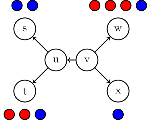
(a) Tree $T$ representing metric $c$

	$\overleftarrow{su}$	$\overleftarrow{tu}$	$\overleftarrow{uv}$	$\overleftarrow{wv}$	$\overleftarrow{xv}$
$\Phi_{c}(A)$	0	2	2	3	0
$\Phi_{c}(B)$	2	1	3	1	1

(b) Embeddings

Figure 1: (1(a)) An assignment problem $(A,B,c)$ with a tree $T$ representing the metric $c$. The elements of $A$ are denoted by $\bullet$ and the elements of $B$ by $\bullet$ and associated to the nodes of $T$ by $\varrho$ as depicted. All edges have weight $1$. (1(b)) Embedding of $A$ and $B$ regarding $T$. The entry $\overleftarrow{uv}$ for the set $B$ counts the total number of $\bullet$ elements associated with the nodes $s$, $t$ and $u$ as indicated by the direction of the edge $uv$ in the tree. The assignment cost is $d^{c}_{\mathrm{oa}}(A,B)=7$.

Note that the roles of $u$ and $v$ are interchangeable and we indicate the choice by directing the edge accordingly. Although this does not affect the assignment cost when applied consistently, there are subtle technical consequences, which we discuss for concrete tree metrics in Section 5.1. Using $T$ and $w$ we can map sets to vectors having a component for every edge of $T$ defined as $\Phi_{c}(S)=\left[\smash{S_{\overleftarrow{uv}}}\cdot w(uv)\right]_{uv\in E(T)}.$ From Eq. 1 it directly follows that the optimal assignment cost are

$$d^{c}_{\mathrm{oa}}(A,B)=\lVert\Phi_{c}(A)-\Phi_{c}(B)\rVert_{1}.$$

This embedding of the optimal assignment cost into $\ell_{1}$ space is used in the following to obtain assignment-based lower bounds on the graph edit distance.

4.2 Embeddable Lower Bounds

Several lower bounds on the graph edit distance can be obtained from optimal assignments [5]. However, these typically do not use a tree metric cost function, which complicates the embedding of assignment costs. In [18] two tree metrics, one based on Weisfeiler-Lehman refinement for graphs with discrete labels and one using clustering for attributed graphs, were introduced. These, however, both do not yield a lower bound. We develop new lower bounds on the graph edit distance from optimal assignment instances, which have a tree metric ground cost function. Most similarity search techniques for the graph edit distance assume a uniform cost model, where every edit operation has the same cost. We also support variable cost functions and discuss choices that are supported by our approach. We use $c_{v}$/$c_{e}$ to denote the costs of inserting or deleting vertices/edges and $c_{vl}$/$c_{el}$ for the costs of changing the respective label.

4.2.1 Vertex Label Lower Bounds

A natural method for defining a lower bound on the graph edit distance is to just take the labels into account ignoring the graph structure. We first discuss the case of uniform cost for changing a label, which is common for discrete labels. Then, non-uniform costs are considered.

Uniform Cost Functions

Clearly, each vertex of one graph, that cannot be assigned to a vertex of the other graph with the same label has to be either deleted or relabeled. The idea leads to a particularly simple assignment instance when we assume fixed costs $c_{vl}$ and $c_{v}$. Let $G$ and $H$ be two graphs with $n$ respectively $m$ vertices. Following the common approach to obtain an assignment instance [29], we extend $G$ by $m$ and $H$ by $n$ dummy nodes denoted by $\epsilon$. We consider the following assignment problem.

Definition 7 (Label Assignment).

The label assignment instance for $G$ and $H$ is given by $(V(G),V(H),c_{\text{llb}})$, where the ground cost function is

$$c_{\text{llb}}(u,v)=\begin{cases}0&\text{ if }\mu(u)=\mu(v)\text{ or }u=v=\epsilon\\ c_{vl}&\text{ if }\mu(u)\neq\mu(v)\\ c_{v}&\text{ if either }u=\epsilon\text{ or }v=\epsilon.\end{cases}$$

We define $\textit{LLB}(G,H)=d^{c_{\text{llb}}}_{\mathrm{oa}}(V(G),V(H))$ and show that it provides a lower bound on the graph edit distance.

Proposition 1 (Label lower bound).

For any two graphs $G$ and $H$, we have $\textit{LLB}(G,H)\leq\textit{GED}(G,H)$.

Proof.

Every assignment directly induces a set of edit operations, which can be arranged to form an edit path. Vice versa, every edit path can be represented by an assignment [29, 5]. Let $\bm{e}$ be a minimum cost edit path. We construct an assignment $f$ from the vertex operations in $\bm{e}$, where the deletion of $v$ is represented by $(v,\epsilon)\in f$, insertion by $(\epsilon,v)\in f$, and relabeling of the vertex $u$ with the label of $v$ by $(u,v)\in f$, where $u,v\neq\epsilon$. We have $c(\bm{e})=Z_{v}+Z_{e}$, where $Z_{v}$ and $Z_{e}$ are the costs of vertex and edge edit operations, respectively. According to the definition of $c_{\text{llb}}$ and the construction of $f$ we have $Z_{v}=c_{\text{llb}}(f)$. An optimal assignment $o$ satisfies $c_{\text{llb}}(o)\leq c_{\text{llb}}(f)$ and $\textit{LLB}(G,H)=c_{\text{llb}}(o)\leq c_{\text{llb}}(f)\leq c(\bm{e})=\textit{GED}(G,H)$ follows, since $Z_{e}\geq 0$. ∎

To obtain embeddings, we investigate for which choices of edit costs the ground cost function $c_{\text{llb}}$ is a tree metric.

Proposition 2 (LLB tree metric).

The ground cost function $c_{\text{llb}}$ is a tree metric if and only if $c_{vl}\leq 2c_{v}$.

Proof.

First we assume $c_{vl}\leq 2c_{v}$ and define a tree $T$ with a central node $r$ having a neighbor for every label $l\in L$ and a neighbor $d$. Let $w(rl)=\tfrac{1}{2}c_{vl}$ for all $l\in L$ and $w(rd)=c_{v}-\tfrac{1}{2}c_{vl}$, cf. Fig. 2(b). The assumption guarantees that all weights are non-negative. We consider the map $\varrho(v)=\mu(v)$ for $v\neq\epsilon$ and $\varrho(\epsilon)=d$. We observe that $c_{\text{llb}}(u,v)=d_{T\!,w}(\varrho(u),\varrho(v))$ by verifying the three cases.

The reverse direction is proven by contradiction. Assume $c_{vl}>2c_{v}$ and $c_{\text{llb}}$ a tree metric. Let $u$ and $v$ be two vertices with $\mu(u)\neq\mu(v)$, then $c_{\text{llb}}(u,v)=c_{vl}$ and $c_{\text{llb}}(u,\epsilon)=c_{\text{llb}}(\epsilon,v)=c_{v}$. Therefore, $c_{\text{llb}}(u,v)>c_{\text{llb}}(u,\epsilon)+c_{\text{llb}}(\epsilon,v)$ contradicting the triangle inequality, Definition 3, (4). Thus, $c_{\text{llb}}$ is not a metric and, in particular, not a tree metric contradicting the assumption. ∎

The requirement $c_{vl}\leq 2c_{v}$ states that relabeling a vertex is at most as expensive as deleting and inserting it with the correct label. This is generally reasonable and not a severe limitation. Because the proof is constructive, it allows us to represent $c_{\text{llb}}$ by a weighted tree, from which we can compute the graph embedding representing the assignment costs following the approach described in Section 4.1.

$G$
$H$

(a) Graphs

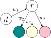
(b) Weighted tree

$\Phi(G)$
$4\cdot w_{1}$
$1\cdot w_{2}$
$1\cdot w_{2}$
$2\cdot w_{2}$

$\Phi(H)$
$4\cdot w_{1}$
$1\cdot w_{2}$
$2\cdot w_{2}$
$1\cdot w_{2}$

(c) Embeddings

Figure 2: Two graphs $G$ and $H$ (2(a)), the weighted tree representing the ground cost function $c_{\text{llb}}$ (2(b)), and the derived embeddings (2(c)). The weights are $w_{1}=c_{v}-\tfrac{1}{2}c_{vl}$ and $w_{2}=\tfrac{1}{2}c_{vl}$. The entries of the vectors correspond to the edges of the tree, from left to right, arrows indicate the direction used when counting elements.

Fig. 2 illustrates the embedding of the label lower bound for an example. The tree representing the cost function is shown in Fig. 2(b). The weight of the edge from the dummy node to the root is chosen, such that the path length from a label to the dummy node is $c_{v}$. Fig. 2(c) shows the vectors $\Phi$ of the two example graphs, which allows obtaining $\textit{LLB}(G,H)=\lVert\Phi(G)-\Phi(H)\rVert_{1}=c_{vl}$ as the Manhattan distance.

Non-Uniform Cost Functions

We have discussed the case where changing one label into another has a fixed cost of $c_{vl}$. In general, the cost for this may depend on the two labels involved, i.e., we assume that a cost function $c_{vl}\colon L\times L\to\mathbb{R}_{\geq 0}$ is given. Two common scenarios can be distinguished: First, $L$ is a (small) finite set of labels that are similar to varying degrees. An example are molecular graphs, where the costs are defined based on vertex labels encoding their pharmacophore properties [12]. Second, $L$ is infinite (or very large), e.g., vertices are annotated with coordinates in $\mathbb{R}^{2}$ and the cost is defined as the Euclidean distance. We propose a general method and then discuss its applicability to both scenarios.

We can extend the tree defining the metric used in the above paragraph to allow for more fine-grained vertex relabel costs. To this end, an arbitrary ultrametric tree on the labels $L$ is defined, where the node $d$ representing deletions is added to its root $r$. Recall that in an ultrametric tree the lengths of all paths from the root to a leaf are equal to, say, $u$. We define the weight of the edge between $r$ and $d$ as $c_{v}-u$ and observe that $c_{v}\geq u$ is required to obtain a valid tree metric in analogy to the proof of Proposition 2.

To obtain an ultrametric tree that reflects the given edit cost function $c_{vl}$, we employ hierarchical clustering. To guarantee that the assignment costs are a lower bound on the graph edit distance, it is crucial that interpreting the hierarchy as an ultrametric tree will underestimate the real edit costs. For optimal results, we would like to obtain a tight lower bound. We formalize the requirements. Let $c_{vl}\colon L{\times}L\to\mathbb{R}_{\geq 0}$ be the given cost function and $d_{hc}\colon L{\times}L\to\mathbb{R}_{\geq 0}$ the ultrametric induced by hierarchical clustering of $L$ with cost function $c_{vl}$. Let $U^{-}\!(c_{vl})$ be the set of all ultrametrics that are lower bounds on $c_{vl}$. There is a unique ultrametric $d^{*}\in U^{-}\!(c_{vl})$ defined as $d^{*}(l_{1},l_{2})=\sup_{d\in U^{-}\!(c_{vl})}\{d(l_{1},l_{2})\}$ for all $l_{1},l_{2}\in L$ [6]. This $d^{*}$ is an upper bound on all ultrametrics in $U^{-}\!(c_{vl})$, a lower bound on $c_{vl}$ and called the subdominant ultrametric to $c_{vl}$. The subdominant ultrametric is generated by single-linkage hierarchical clustering [6], which therefore is, in this respect, optimal for our purpose. In particular, it reconstructs an ultrametric tree if the original costs are ultrametric. Moreover, single-linkage clustering can be implemented with running time $O({L}^{2})$ [36].

For a finite set of labels $L$, our method is a viable solution if the edit cost function $c_{vl}$ is close to an ultrametric and $L$ is small. If $L$ is infinite, we need to approximate it with a finite set through quantization or space partitioning. The realization of such an approach preserving the lower bound property depends on the specific application and is hence not further explored here.

4.2.2 Degree Lower Bound

The LLB does not take the graph structure into account. We now introduce the degree lower bound, which focuses on how many edges have to be inserted or deleted at the minimum. When deleting or inserting vertices, all of the adjacent edges have to be deleted or inserted as well. If two vertices with differing degrees are assigned to one another, again edges have to be deleted or inserted accordingly. As in Section 4.2.1, we extend the graphs $G$ and $H$ by dummy nodes $\epsilon$ and define an assignment problem.

Definition 8 (Degree Assignment).

The degree assignment instance for $G$ and $H$ is given by $(V(G),V(H),c_{\text{dlb}})$, where the ground cost function is $c_{\text{dlb}}(u,v)=\tfrac{1}{2}c_{e}\mid\delta(u)-\delta(v)\mid$ with $\delta(\epsilon):=0$ for the dummy nodes.

We define $\textit{DLB}(G,H)=d^{c_{\text{dlb}}}_{\mathrm{oa}}(V(G),V(H))$, and show that it is a lower bound.

Proposition 3 (Degree lower bound).

For any two graphs $G$ and $H$, we have $\textit{DLB}(G,H)\leq\textit{GED}(G,H)$.

Proof.

Using the same arguments as in the proof of Proposition 2, let $\bm{e}$ be a minimum cost edit path and $f$ an assignment that induces $\bm{e}$. We divide the costs $c(\bm{e})=Z_{v}{+}Z_{e}$ into costs $Z_{v}$ and $Z_{e}$ of vertex and edge edit operations. For the matched vertices $v$ and $f(v)$ at least $\mid\delta(v)-\delta(f(v))\mid$ edges must be deleted or inserted to balance the degrees; in case of insertion and deletion all adjacent edges must be inserted or deleted. Since each edge edit operation increases or decreases the degree of its two endpoints by one, the sum of these costs over all vertices must be divided by two and $c_{\text{dlb}}(f)=Z_{e}$ follows. ∎

To obtain an embedding, we show that $c_{\text{dlb}}$ is a tree metric.

Proposition 4 (DLB tree metric).

The ground cost function $c_{\text{dlb}}$ is a tree metric.

Proof.

To prove that $c_{\text{dlb}}$ is a tree metric, we construct a tree $T$ with edge weights $w$ and a map $\varrho$, so that $c_{\text{dlb}}(u,v)=d_{T\!,w}(\varrho(u),\varrho(v))$. Let $T$ have nodes $V(T)=\{r=0,1,\dots,\Delta\}$ and edges $E(T)=\{ij\mid j=i{+}1\}$ with weight $w_{1}=\tfrac{1}{2}c_{e}$. Since $c_{e}$ cannot be negative, all edge weights are non-negative. We consider the map

$$\varrho(u)=\begin{cases}r&\text{if }u=\epsilon\text{ or }\delta(u)=0\\ \delta(u)&\text{otherwise.}\\ \end{cases}$$

It can easily be seen, that $c_{\text{dlb}}(u,v)=d_{T\!,w}(\varrho(u),\varrho(v))$ by verifying the path lengths in the tree. ∎

The proof gives a concept to construct a tree representing the DLB cost function. As there is no difference between a vertex with degree 0 and a dummy vertex, they can both be assigned to the root node $r$. Note, that the edge labels are not taken into account by this lower bound and edge insertion and deletion are not distinguished. Fig. 3 illustrates the embedding of the degree lower bound, which yields $\textit{DLB}(G,H)=c_{e}$ for the running example.

$G$
$H$

(a) Graphs

(b) Weighted tree

$\Phi(G)$
$4\cdot w_{1}$
$3\cdot w_{1}$
$1\cdot w_{1}$

$\Phi(H)$
$4\cdot w_{1}$
$4\cdot w_{1}$
$0\cdot w_{1}$

(c) Embeddings

Figure 3: Two graphs $G$ and $H$ (3(a)), the weighted tree representing the cost function $c_{\text{dlb}}$ (3(b)), and the derived embeddings (3(c)).

4.2.3 Combined Lower Bound

We can combine LLB and DLB to improve the approximation.

Definition 9 (CLB).

The combined lower bound between $G$ and $H$ is defined as $\textit{CLB}(G,H)=\textit{LLB}(G,H)+\textit{DLB}(G,H).$

We show, that CLB is a lower bound on the graph edit distance. Note that this lower bound is based on the two assignments given by LLB and DLB, which are not necessarily equal.

Lemma 1.

Let $c_{1},c_{2}$ and $c$ be ground cost functions on $X$ and $c(x,y)=c_{1}(x,y)+c_{2}(x,y)$ for all $x,y\in X$. Then for any $A,B\subseteq X$, ${A}={B}=n$, the inequality $d^{c_{1}}_{\mathrm{oa}}(A,B)+d^{c_{2}}_{\mathrm{oa}}(A,B)\leq d^{c}_{\mathrm{oa}}(A,B)$ holds.

Proof.

Let $o_{1},o_{2}$ and $o$ be optimal assignments between $A$ and $B$ regarding the ground costs $c_{1},c_{2}$ and $c$, respectively. Due to the optimality we have $c_{1}(o_{1})\leq c_{1}(o)$ and $c_{2}(o_{2})\leq c_{2}(o)$. Hence, $d^{c_{1}}_{\mathrm{oa}}(A,B)+d^{c_{2}}_{\mathrm{oa}}(A,B)=c_{1}(o_{1})+c_{2}(o_{2})\leq c_{1}(o)+c_{2}(o)=c(o)=d^{c}_{\mathrm{oa}}(A,B)$. ∎

Proposition 5 (Combined lower bound).

For any two graphs $G$ and $H$, we have $\textit{CLB}(G,H)\leq\textit{GED}(G,H)$.

Proof.

Let $\bm{e}$ be a minimum cost edit path and $f$ an assignment that induces $\bm{e}$. We divide the costs $c(\bm{e})=Z_{v}+Z_{e}$ into costs $Z_{v}$ and $Z_{e}$ of vertex and edge edit operations. From the proof of Propositions 1 and 3 we know that $Z_{v}\geq c_{\text{llb}}(f)$ and $Z_{e}\geq c_{\text{dlb}}(f)$ and, hence, $c(\bm{e})\geq c_{\text{llb}}(f)+c_{\text{dlb}}(f)$. Application of Lemma 1 yields $\textit{CLB}(G,H)=c_{\text{llb}}(f_{1})+c_{\text{dlb}}(f_{2})\leq c_{\text{llb}}(f)+c_{\text{dlb}}(f)\leq c(\bm{e})=\textit{GED}(G,H)$, where $f_{1}$ and $f_{2}$ are optimal assignments regarding $c_{\text{llb}}$ and $c_{\text{dlb}}$. ∎

This lower bound is at least as tight as the ones it consists of and, therefore, most promising. The combined lower bound is embedded by concatenating the vectors for LLB and DLB.

4.3 Analysis

We provide a theoretical comparison of our proposed bounds to existing lower bounds and also give details on the time complexity of our approach.

4.3.1 Comparison with Existing Bounds

We relate the CLB to two well-known lower bounds when applied to graphs with vertex labels. The simple label filter (SLF) is the intersection of vertex and edge label multisets, i.e., $\textit{SLF}(G,H)={L_{V}(G)\cap L_{V}(H)}+{{E(G)}-{E(H)}}$ in our case, where $L_{V}$ denotes the vertex label multiset of a graph. Although simple, this bound is often found to be selective [15] and, therefore, widely-used [44, 45]. A very effective bound according to [5] is BranchLB based on general optimal assignments. Several variants have been proposed [29, 46, 5] with at least cubic worst-case time complexity. In our case, BranchLB is the cost of the optimal assignment regarding the ground costs $c_{\text{branch}}(u,v)=c_{\text{llb}}(u,v)+c_{\text{dlb}}(u,v)$. Note that $c_{\text{branch}}$ in general is not a tree metric. SLF assumes $c_{v}=c_{vl}=c_{e}=1$ and we consider this setting although CLB and BranchLB are more general. Using counting arguments and Lemma 1 we obtain the following relation:

Proposition 6.

For any two vertex-labeled graphs $G$ and $H$,

$$\textit{SLF}(G,H)\,{\leq}\,\textit{CLB}(G,H)\,{\leq}\,\textit{BranchLB}(G,H)\,{\leq}\,\textit{GED}(G,H).$$

Experimentally we show in Section 6 that our combined lower bound is close to BranchLB for a wide-range of real-world datasets, but is computed several orders of magnitude faster and allows indexing. This makes it ideally suitable for fast pre-filtering and search.

4.3.2 Time Complexity

We first consider the time required for generating the vector $\Phi_{c}(S)$ for a set $S$ and tree $T$ defining the ground cost function $c$.

Proposition 7.

Given a set $S$ and a weighted tree $T$ representing the ground cost function $c$, the vector $\Phi_{c}(S)$ can be computed in $O({V(T)}+{S})$ time.

Proof.

We first associate the elements of $S$ with the nodes of $T$ via the map $\varrho$ and then traverse $T$ starting from the leaves progressively moving towards the center. The order guarantees that when the node $u$ is visited, exactly one of its neighbors, say $v$, has not yet been visited. Then $S_{\overleftarrow{uv}}$ can be obtained as $\sum_{w\in N(u)\setminus\{v\}}S_{\overleftarrow{wu}}$ from the values computed previously. The tree traversal and computation of $S_{\overleftarrow{uv}}$ for all $uv\in E(T)$ takes $O({V(T)})$ total time. Together with the time for processing the set $S$ we obtain $O({V(T)}+{S})$ time. ∎

The time complexity of the different bounds depends on the size of the tree representing the metric and the size of the graphs.

Proposition 8.

The bounds $c_{\text{llb}}$, $c_{\text{dlb}}$ and $c_{\text{clb}}$ for two graphs $G$ and $H$ can be computed in $O({V(G)}+{V(H)})$ time.

Proof.

First the tree $T$ defining the metric is computed. For the different tree metrics, the trees sizes are linear in the number of nodes of the two graphs $G$ and $H$: For $c_{\text{llb}}$ the tree (denoted $T_{\text{llb}}$) has size ${L_{v}(G)\cup L_{v}(H)}+2$, where $L_{v}(G)$ denotes the set of vertex labels occurring in $G$. The tree consists of a node for each vertex label plus a dummy and a central node. In the worst case, where all labels occur only once, the tree is of size ${V(G)}+{V(H)}+2$. For $c_{\text{dlb}}$, we have ${V(T_{\text{dlb}})}=\max(\delta(G),\delta(H))+1$, since there is a node for each vertex degree, up to the maximum degree (including degree $0$). As shown in Proposition 7, the vector $\Phi_{c}(G)$ can then be computed in time $O({V(T)}+{V(G)})$. For $c_{\text{clb}}$ we concatenate the vectors of $c_{\text{llb}}$ and $c_{\text{dlb}}$. The Manhattan distance between two vectors is computed in time linear in the number of components, which is $O({V(T)})$. Thus, the total running time for computing any of the bounds is in $O({V(G)}+{V(H)})$.

∎

The bound SLF also has a linear time complexity while BranchLB requires $O(n^{2}\Delta^{3}+n^{3})$ time for graphs with $n$ vertices and maximum degree $\Delta$ [5]. Our new approach matches the running time of SLF but in most cases yields tighter bounds, cf. Proposition 6 and our experimental evaluation in Section 6. Hence, it provides a favorable trade-off between efficiency and quality and at the same time can conveniently be combined with indices.

5 EmbAssi for Graph Similarity Search

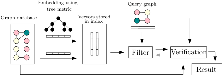
Figure 4: Overview of our pipeline for graph similarity search. In a preprocessing step the embeddings of all database graphs under the specified tree metric are computed and stored in an index. Then similarity search queries are answered by computing the embedding of the query graph and filtering regarding the Manhattan distance. In $k$-nearest neighbor search, the information gained from refining candidates is used to reduce the search range. This is indicated with a gray arrow.

We use the proposed lower bounds for similarity search by computing embeddings for all the graphs in the database in a preprocessing step. Given a query graph, we compute its embedding and realize filtering utilizing indices regarding the Manhattan distance. The approach is illustrated in Fig. 4. Algorithm 1 shows how the preprocessing is done, exemplary for LLB: We construct the tree metric based on the labels and associate the vertices with the leaves of the tree. Then for each graph the embedding is computed using Algorithm 2.

Several technical details must be considered. The choice of how to direct the edges has a huge impact on the resulting vectors and of course using a suitable index is also important. In the following, we briefly discuss our choices and explain how similarity search queries can be answered.

Algorithm 1 Construction for LLB

procedure constructIndex(set of graphs $DB$)

     $T$ $\leftarrow$ new tree with root $\epsilon$ and child $r$

     $w((\epsilon,r))\leftarrow c_{v}-\tfrac{1}{2}c_{vl}$ $\triangleright$ Set edge weight

     for all $G\in DB$ do $\triangleright$ Construct tree metric LLB

         for all $v\in V(G)$ do

              if $\mu(v)\notin T$ then

                  add node $\mu(v)$ as child of $r$ with $w((r,\mu(v)))=\tfrac{1}{2}c_{vl}$

                  $\varrho(v)\leftarrow\mu(v)$

              end if

         end for

     end for

     for all $G\in DB$ do $\triangleright$ Compute embedding under tree metric

         $\Phi(G)\leftarrow$ computeVector($G$, $T$)

     end for

     Create index($\{\Phi(G)\mid G\in DB\}$, Manhattan distance)

end procedure

Algorithm 2 Vector Computation

procedure computeVector(graph $G$, tree $T$)

     $\Phi(G)\leftarrow$ sparse vector

     $S\leftarrow$ relevant subtree$(V(G),T)$ $\triangleright$ $\forall v\in V(G):$ $\varrho(v)$ and path to root

     $count[n]\leftarrow 0,\forall n\in V(S)$

     for all $v\in V(G)$ do

         $count[\varrho(v)]\leftarrow count[\varrho(v)]+1$ $\triangleright$ Count vertices at leaves

     end for

     $leaves\leftarrow$ leaves of $S$

     while $l\leftarrow leaves$.dequeue() and $l\neq$ root of $S$ do

         $\Phi(G)[(l,p)]\leftarrow w((l,p))\cdot count[l]$

         $count[p]=count[p]+count[l]$ $\triangleright$ Propagate vertex count to parent

         delete $l$ from $S$

         if $\delta(p)\leq 1$ then $\triangleright$ $p$ is now a leaf itself

              $leaves$.enqueue($p$)

         end if

     end while

     return $\Phi(G)$

end procedure

5.1 Index Construction

We compute the vectors for all graphs in the database and store them in an index to accelerate queries. When defining the bounds, we considered the pairwise comparison of two graphs and added dummy vertices to obtain graphs of the same size. We have chosen the direction of edges in the trees representing the metrics carefully, cf. Section 4.1, to generate consistent embeddings for the entire database. By rooting the trees at the node $\varrho(\epsilon)$ representing the dummy vertices (see Algorithm 1) and directing all edges towards the leaves the dummy vertices are not counted in any entry of the vectors, see Fig. 2--3. Moreover, this choice often leads to sparse vectors, e.g., for the LLB, where every entry just counts the number of vertices with one specific label. Labels that only appear in a small fraction of the graphs in the database then lead to zero-entries in the vectors of the other graphs and sparse data structures become beneficial. Moreover, this simplifies to dynamically add new vertex labels without requiring to update all existing vectors in the database. Using sparse vector representations, Algorithm 2 can be implemented in time $O({V(G)})$ by considering only the relevant part of $T$. This is the subtree $S$ formed by the nodes of $T$ to which vertices of $G$ are assigned to via $\varrho$, and the nodes on the path to the root from these nodes. The subtree $S$ is processed in a bottom-up fashion computing a non-zero component of $\Phi(G)$ in each step. Note that $S$ can be maintained and modified with low overhead using flags to indicate whether a node of $T$ is contained in $S$.

The choice of a suitable index is crucial for the performance of our approach. We chose to use the cover tree [4] because our data is too high-dimensional for the popular k-d-tree, and our vectors have many zeros and discrete values. The cover tree is a good choice for an in-memory index because of its lightweight construction, low memory requirements, and good metric pruning properties. It is usually superior to the k-d-tree or R-tree if the data stored is high-dimensional but still has a small doubling dimension.

5.2 Queries

For similarity search, we compute the embedding of the query graph and use the index for similarity search regarding Manhattan distance. The index takes responsibility to disregard parts of the database that are too far away from the query object. In $k$-nearest neighbor search, we use the optimal multi-step $k$-nearest neighbor search [34] as described in Section 3.3 to stop the search as early as possible and compute the minimum necessary number of exact graph edit distances. Our lower bounds are especially useful for this because it is well understood how to index data for ranking by Manhattan distance. Further exact distance computations (in particular for range queries) can be avoided by checking additional bounds similar to Inves [15] or BSS_GED [9] prior to an exact distance computation.

A tighter (but more expensive) lower bound produces fewer candidates, while in some applications (such as DBSCAN clustering), where the exact distance is not necessary to have, an upper bound can identify true positives efficiently.

6 Experimental Evaluation

In this section, we compare EmbAssi to state-of-the-art approaches regarding efficiency and approximation quality in range and $k$-nearest neighbor queries. We investigate the speed-up of existing filter-verification pipelines when EmbAssi is used in a pre-filtering step. Specifically, we address the following research questions:

• How tight are our lower bounds compared to the state-of-the-art? How do our bounds perform when taking the trade-off between bound quality and runtime into account?

• Can EmbAssi compete with state-of-the-art methods in terms of runtime and selectivity? Is CLB a suitable lower bound to provide initial candidates for range queries?

• Can EmbAssi perform similarity search on datasets with a million graphs or more?

• Can $k$-nearest neighbor queries be answered efficiently?

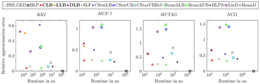
Figure 5: Comparison of several different approximations regarding their relative approximation error and runtime.
$\square$: exact approach, $\circ$: upper bound, $\times$: existing lower bound, $\triangle$: newly proposed lower bound from tree metric.

6.1 Setup

This section gives an overview of the datasets, the methods, and their configuration used in the experimental comparison.

Methods and Distance Functions. We compare EmbAssi to GSim [44] and MLIndex [23], which are representative methods for similarity search based on overlapping substructures and graph partitioning. MLIndex is considered as state-of-the-art [28], although we observed that GSim often performs much better. We also compare to CStar [43] and Branch [5], which provide both upper and lower bounds on the graph edit distance, but are not accelerated with indices. Furthermore, we compare to the exact graph edit distance BLP [21], BSS_GED [9], and the approximations LinD [18], BLPlb [5] and BeamS [27] regarding the approximation of the GED. The costs of all edit operations were set to one because some of the comparison methods only support uniform costs. For BeamD, we used a maximum list size of 100. For LinD, the tree was generated using the Weisfeiler-Lehman algorithm with one refinement iteration. For GSim, we used all provided filters and $q=3$. For MLIndex, the default settings of the authors’ implementation were used.

Table 2: Distance functions compared in the experiments

Name	Description	Bound	Source
BLP	Exact graph edit distance	exact	[21]
BSS_GED	Efficient ged computation/verification	exact	[9]
BeamD	Approximation using BeamSearch	upper	[27]
LinD	Optimal assignments with WL	upper	[18]
BranchUB	Cost of edit path gained from BranchLB	upper	[5]
CStarUB	Optimal assignments with stars	upper	[43]
CStarUBRef	Refined Version of CStarUB	upper	[43]
CStarLB	Mapping distance between stars	lower	[43]
SLF	Min. label changes	lower	[15]
BranchLB	Modification of BP	lower	[5]
BLPlb	Relaxation of BLP	lower	[5]
New distance functions based on tree metrics
LLB	Min. vertex label changes	lower	new
DLB	Min. edge insertion/deletions	lower	new
CLB	LLB and DLB combined	lower	new

The bounds computed by CStar can also be used separately and will be referred to as CStarLB, CStarUB, and CStarUBRef, which is obtained by improving an edit path using local search. SLF and BranchLB are the lower bounds discussed in Section 4.2.3 and were implemented following the description in [15] and [5], respectively. BranchLB and the upper bound gained from the edit path induced by it (BranchUB) are referred to as Branch when applied together. Table 2 gives an overview of the distance functions compared in the experiments including those known from literature as well as those proposed here for use with EmbAssi. The graphs and their respective vectors are indexed using the cover tree [4] implementation of the ELKI framework [31].

Datasets.

Table 3: Datasets with discrete vertex labels and their statistics [24]. ChEMBL (chembl_27, [13]) contains small molecules, Protein Com contains protein complex graphs [37].

Name	$|$Graphs$|$	avg $|V|$	avg $|E|$	avg $\delta(v)$	$|L|$
KKI	$83$	$26.96$	$48.42$	$3.59$ $\pm 2.58$	$190$
MCF-7	$27770$	$26.08$	$28.29$	$2.16$ $\pm 0.76$	$23$
MUTAG	$188$	$17.93$	$19.79$	$2.20$ $\pm 0.74$	$7$
NCI1	$4110$	$29.04$	$31.61$	$2.16$ $\pm 0.78$	$21$
PTC_FM	$349$	$14.11$	$14.48$	$2.05$ $\pm 0.81$	$18$
Protein Com	$1455324$	$9.98$	$8.98$	$1.80$ $\pm 3.03$	$717$
ChEMBL	$1941411$	$30.18$	$32.71$	$2.15$ $\pm 0.74$	$31$

We tested all methods on a wide range of real-world datasets with different characteristics, see Table 3. The datasets have discrete vertex labels. Edge labels and attributes, if present, were removed prior to the experiments since not all methods support them. Also, since MLIndex and GSim do not work for disconnected graphs, only their largest connected components were used.

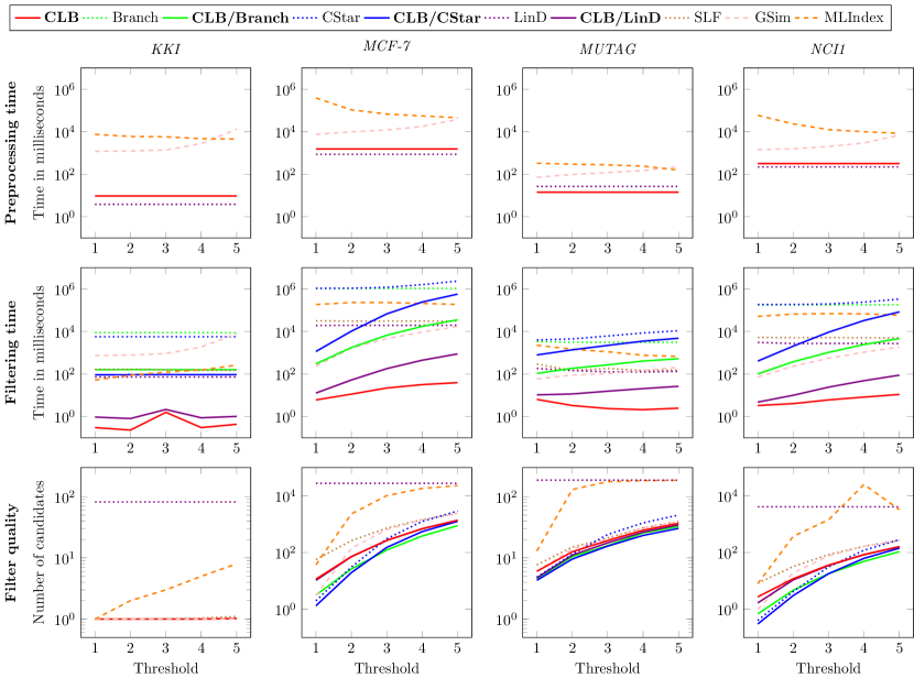
Figure 6: Runtime and selectivity comparison of different filters. Preprocessing time, filtering time for 50 range queries (excluding verification), and the average number of candidates, that need to be verified, is shown. For the methods, that can be enhanced using EmbAssi, the solid line shows the advantage of pre-filtering with CLB, while the dotted line is the original approach.

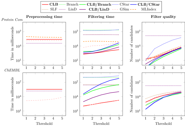
Figure 7: Comparison of several different filters regarding their selectivity and runtime on datasets Protein Com and ChEMBL. The solid lines show the advantage of using EmbAssi with CLB as a pre-filter, while the dotted lines show the original approaches.

6.2 Results

In the following, we report on our experimental results and discuss the different research questions.

Q1: Bound Quality and Runtime. Accuracy is crucial to obtain effective filters for similarity search. We investigate how tight the proposed lower bounds on the graph edit distance are. Fig. 5 shows the average relative approximation error $\frac{{\text{GED}-d_{\text{approx}}}}{\text{GED}}$ of the different bounds in comparison to their runtime. The newly proposed bounds, as well as SLF, are very fast, with varying degrees of accuracy. Although CLB is much faster than BranchLB, its accuracy is in many cases on par or only slightly worse. Note that a timeout of 120 seconds per graph pair was used for the computation of the exact graph edit distance for this experiment. For this reason, values for BSS_GED are not present for the datasets with larger graphs.

Q2: Evaluation of Runtime and Selectivity. The runtime of the algorithms consists of three parts: (1) preprocessing and indexing, (2) filtering, and (3) verification. Preprocessing and indexing is performed only once, and this cost amortizes over many queries, while the time required to determine the candidate set and its size are crucial. The verification step requires to compute the exact graph edit distance and is usually most expensive and essentially depends on the number of candidates.

In the following, we investigate how well EmbAssi performs on range queries, how much of a speed-up can be achieved for existing pipelines when filtering with EmbAssi first, and compare to state-of-the-art approaches. We omit bounds that were shown in the previous experiments to have a poor accuracy or a very high runtime. Fig. 6 shows the runtime for preprocessing, filtering and the average number of candidates per query for range queries with thresholds 1 to 5. The solid lines show the results, when using EmbAssi with CLB as a first filter, while the dotted line represent the original approaches. The solid red line shows the results using only EmbAssi with CLB and no further filters. GSim and MLIndex are shown with dashed lines, since they are stand-alone approaches. These two methods skip database graphs that are smaller than the given threshold. To obtain a valid candidate set, these graphs were added back after filtering. For GSim and MLIndex the preprocessing time is rather high and highly dependent on the maximum threshold for range search, which must be chosen in advance.

It becomes evident that EmbAssi significantly accelerates all methods across the various datasets. The preprocessing and filtering time of EmbAssi is very low: While filtering only takes a few milliseconds, preprocessing ranges from 0.01 to 2 seconds over the various datasets. $CStar$ and $Branch$ have the best selectivity, but they also employ both upper and lower bounds and need more time for filtering. The usage of EmbAssi heavily accelerates both methods, while even increasing the selectivity of $CStar$ (as seen in Fig. 5, $CStarLB$ seems to be looser than CLB in general). Note, that LinD is an upper bound, so the candidate set consist of all graphs, that could not be reported as a result. In combination with EmbAssi it is only slightly worse than the other approaches regarding filter selectivity, while being very fast.

Considering the properties of the datasets and the performance, we observe that a larger set of vertex labels and a high variance among the vertex degrees seem to lead to a better filter quality. The larger the graphs, the greater the improvement in runtime during the filtering step.

Since competing approaches do not use the fast verification algorithm BSS_GED [9] a comparison of verification time would not be fair. On the various datasets the time for verification (of 50 queries with threshold 5) using the candidates of CLB ranged from around $35$ms (KKI) to a maximum of $5$s (MCF-7).

Combining these results, we can conclude that EmbAssi is well suited as pre-filtering for more effective computational demanding bounds. EmbAssi substantially reduces the filtering time and promises scalability even to very large datasets. We investigate this below.

Q3: Similarity Search on Very Large Datasets. We investigate how well EmbAssi performs on very large graph databases using the datasets Protein Com and ChEMBL. Fig. 7 shows the average number of candidates per query as reported by the different methods, as well as the time needed for preprocessing and filtering. MLIndex did not finish on ChEMBL within a time limit of 24 hours (for threshold 1). For dataset Protein Com our new approach is not only much faster, but also provides a better filter quality than state-of-the-art methods. It can clearly be seen, that EmbAssi with CLB provides a substantial boost in runtime, while also improving the filter quality.

Q4: $k$-Nearest-Neighbor Search. An advantage of EmbAssi is that it can also answer $k$-nn queries efficiently due to the use of the multi-step $k$-nearest neighbor search algorithm as described in Section 3.3. Table 4 compares the average number of candidates generated using EmbAssi (with CLB) and BranchLB, as well as the average time needed for answering a $k$-nn query. In both methods, candidate sets were verified using the faster exact graph edit distance computation BSS_GED. The last column shows the average number of nearest neighbors reported, which may be larger than $k$ because of ties.

Table 4: Runtime and number of candidates in $k$-nearest-neighbor search using EmbAssi and BranchLB.

	$k$	EmbAssi		BranchLB		$|$NN$|$
		$|$Cand$|$	Time (sec)	$|$Cand$|$	Time (sec)
PTC_FM	1	14.40	0.24	9.00	1.42	1.20
	2	24.40	0.42	19.60	1.34	3.40
	3	28.40	0.43	22.20	1.16	4.40
	4	31.80	1.06	25.20	1.40	5.60
	5	39.00	1.19	31.20	1.24	6.60
MUTAG	1	6.80	0.15	6.80	0.87	1.60
	2	9.80	0.22	9.80	0.99	3.80
	3	14.00	0.25	14.00	1.31	5.80
	4	14.00	0.49	14.00	1.03	5.80
	5	15.80	0.55	15.80	1.08	7.40
MCF-7	1	659.67	48.04	434.33	191.95	1.33
	2	1114.33	152.43	737.00	244.42	2.33
	3	1610.00	214.64	1045.67	410.11	4.00
	4	1968.33	391.37	1380.33	577.75	10.00
	5	2401.00	642.29	1696.33	678.06	10.67

It can be seen, that EmbAssi provides a runtime advantage in $k$-nearest neighbor search, and the number of candidates generated is not much higher than when using BranchLB. For larger datasets, we expect the advantage of EmbAssi to be more significant. Further optimization of the approach is possible. For example, it might be beneficial to combine both methods and use EmbAssi in combination with tighter lower bounds such as BranchLB to reduce the number of exact graph edit distance computations.

7 Conclusions

We have proposed new lower bounds on the graph edit distance, which are efficiently computed, readily combined with indices, and fairly selective in filtering. This makes them ideally suitable as a pre-filtering step in existing filter-verification pipelines that do not scale to large databases. Our approach supports efficient $k$-nearest neighbor search using the optimal multi-step $k$-nearest neighbor search algorithm unlike many comparable methods. Other methods have to first perform a range query with a sufficient range and find the $k$-nearest neighbors among those candidates.

An interesting direction of future work is the combination and development of indices for computational demanding lower bounds such as those obtained from general assignment problems or linear programming relaxations. Efficient methods for similarity search regarding the Wasserstein distance have only recently been investigated [1]. Moreover, approximate filter techniques for the graph edit distance based on embeddings learned by graph neural networks were only recently proposed [28]. With the increasing amount of structured data, scalability is a key issue in graph similarity search.

References

- Backurs et al. [2020] A. Backurs, Y. Dong, P. Indyk, I. Razenshteyn, and T. Wagner. Scalable nearest neighbor search for optimal transport. In Int. Conf. Machine Learning, ICML, volume 119, pages 497--506, 2020.
- Bai et al. [2019] Y. Bai, H. Ding, S. Bian, T. Chen, Y. Sun, and W. Wang. SimGNN: A neural network approach to fast graph similarity computation. In ACM International Conference on Web Search and Data Mining, WSDM, 2019. ISBN 978-1-4503-5940-5. 10.1145/3289600.3290967.
- Bause et al. [2021] F. Bause, D. B. Blumenthal, E. Schubert, and N. M. Kriege. Metric indexing for graph similarity search. In SISAP 2021, volume 13058 of Lecture Notes in Computer Science, 2021. 10.1007/978-3-030-89657-7_24.
- Beygelzimer et al. [2006] A. Beygelzimer, S. M. Kakade, and J. Langford. Cover trees for nearest neighbor. In Int. Conf. Machine Learning, ICML, volume 148, 2006. 10.1145/1143844.1143857.
- Blumenthal et al. [2019] D. Blumenthal, N. Boria, J. Gamper, S. Bougleux, and L. Brun. Comparing heuristics for graph edit distance computation. The VLDB Journal, 07 2019. 10.1007/s00778-019-00544-1.
- Bock [1974] H. H. Bock. Automatische Klassifikation. Vandenhoeck & Ruprecht, 1974. ISBN 978-3525401309.
- Burkard et al. [2012] R. E. Burkard, M. Dell’Amico, and S. Martello. Assignment Problems. SIAM, 2012. 10.1137/1.9781611972238.
- Chang et al. [2020] L. Chang, X. Feng, X. Lin, L. Qin, W. Zhang, and D. Ouyang. Speeding up GED verification for graph similarity search. In Int. Conf. Data Engineering, ICDE, pages 793--804, 2020. 10.1109/ICDE48307.2020.00074.
- Chen et al. [2019] X. Chen, H. Huo, J. Huan, and J. S. Vitter. An efficient algorithm for graph edit distance computation. Knowledge-Based Systems, 163:762--775, 2019. ISSN 0950-7051. https://doi.org/10.1016/j.knosys.2018.10.002.
- Duan and Su [2012] R. Duan and H.-H. Su. A scaling algorithm for maximum weight matching in bipartite graphs. In Symposium on Discrete Algorithms, SODA, 2012. 10.1137/1.9781611973099.111.
- Ester et al. [1996] M. Ester, H. Kriegel, J. Sander, and X. Xu. A density-based algorithm for discovering clusters in large spatial databases with noise. In Int. Conf. Knowledge Discovery and Data Mining (KDD), pages 226--231, 1996.
- Garcia-Hernandez et al. [2019] C. Garcia-Hernandez, A. Fernández, and F. Serratosa. Ligand-based virtual screening using graph edit distance as molecular similarity measure. J. Chem. Inf. Model., 59(4):1410--1421, 2019. 10.1021/acs.jcim.8b00820.
- Gaulton et al. [2016] A. Gaulton, A. Hersey, M. Nowotka, A. P. Bento, J. Chambers, D. Mendez, P. Mutowo, F. Atkinson, L. J. Bellis, E. Cibrián-Uhalte, M. Davies, N. Dedman, A. Karlsson, M. P. Magariños, J. P. Overington, G. Papadatos, I. Smit, and A. R. Leach. The ChEMBL database in 2017. Nucleic Acids Research, 45(D1):D945--D954, 11 2016. ISSN 0305-1048. 10.1093/nar/gkw1074.
- Gouda and Hassaan [2016] K. Gouda and M. Hassaan. CSI_GED: An efficient approach for graph edit similarity computation. In Int. Conf. Data Engineering, ICDE, 2016. 10.1109/ICDE.2016.7498246.
- Kim et al. [2019] J. Kim, D. Choi, and C. Li. Inves: Incremental partitioning-based verification for graph similarity search. In EDBT, pages 229--240, 2019. 10.5441/002/edbt.2019.21.
- Kriege et al. [2016] N. M. Kriege, P. Giscard, and R. C. Wilson. On valid optimal assignment kernels and applications to graph classification. In Advances in Neural Information Processing Systems, pages 1615--1623, 2016.
- Kriege et al. [2018] N. M. Kriege, M. Fey, D. Fisseler, P. Mutzel, and F. Weichert. Recognizing cuneiform signs using graph based methods. In Int. Workshop on Cost-Sensitive Learning, COST@SDM, volume 88 of PMLR, 2018.
- Kriege et al. [2019] N. M. Kriege, P. Giscard, F. Bause, and R. C. Wilson. Computing optimal assignments in linear time for approximate graph matching. In ICDM, pages 349--358, 2019. 10.1109/ICDM.2019.00045.
- Kriege et al. [2020] N. M. Kriege, F. D. Johansson, and C. Morris. A survey on graph kernels. Appl. Netw. Sci., 5(1):6, 2020. 10.1007/s41109-019-0195-3.
- Le et al. [2019] T. Le, M. Yamada, K. Fukumizu, and M. Cuturi. Tree-sliced variants of Wasserstein distances. In Neural Information Processing Systems, 2019.
- Lerouge et al. [2017] J. Lerouge, Z. Abu-Aisheh, R. Raveaux, P. Héroux, and S. Adam. New binary linear programming formulation to compute the graph edit distance. Pattern Recognit., 72:254--265, 2017. 10.1016/j.patcog.2017.07.029.
- Li et al. [2019] Y. Li, C. Gu, T. Dullien, O. Vinyals, and P. Kohli. Graph matching networks for learning the similarity of graph structured objects. In ICML, 2019.
- Liang and Zhao [2017] Y. Liang and P. Zhao. Similarity search in graph databases: A multi-layered indexing approach. In Int. Conf. Data Engineering, ICDE, 2017. 10.1109/ICDE.2017.129.
- Morris et al. [2020] C. Morris, N. M. Kriege, F. Bause, K. Kersting, P. Mutzel, and M. Neumann. TUDataset: A collection of benchmark datasets for learning with graphs. In ICML Workshop on Graph Representation Learning and Beyond, GRL+, 2020.
- Munkres [1957] J. R. Munkres. Algorithms for the assignment and transportation problems. J. Soc. Ind. Appl. Math., 5(1):32--38, 1957.
- Nasr et al. [2010] R. Nasr, D. S. Hirschberg, and P. Baldi. Hashing algorithms and data structures for rapid searches of fingerprint vectors. J. Chem. Inf. Model., 50(8):1358--1368, 2010. 10.1021/ci100132g.
- Neuhaus et al. [2006] M. Neuhaus, K. Riesen, and H. Bunke. Fast suboptimal algorithms for the computation of graph edit distance. In Structural, Syntactic, and Statistical Pattern Recognition, pages 163--172, 08 2006. 10.1007/11815921_17.
- Qin et al. [2020] Z. Qin, Y. Bai, and Y. Sun. GHashing: Semantic graph hashing for approximate similarity search in graph databases. In ACM SIGKDD, pages 2062--2072, 2020.
- Riesen and Bunke [2009] K. Riesen and H. Bunke. Approximate graph edit distance computation by means of bipartite graph matching. Image Vision Comput., 27(7):950--959, 2009. 10.1016/j.imavis.2008.04.004.
- Riesen et al. [2015] K. Riesen, M. Ferrer, A. Fischer, and H. Bunke. Approximation of graph edit distance in quadratic time. In Graph-Based Representations in Pattern Recognition, pages 3--12, 2015. ISBN 978-3-319-18224-7.
- Schubert and Zimek [2019] E. Schubert and A. Zimek. ELKI: A large open-source library for data analysis - ELKI release 0.7.5 Heidelberg. CoRR, abs/1902.03616, 2019.
- Schubert et al. [2014] E. Schubert, A. Zimek, and H. Kriegel. Local outlier detection reconsidered: a generalized view on locality with applications to spatial, video, and network outlier detection. Data Min. Knowl. Discov., 28(1):190--237, 2014. 10.1007/s10618-012-0300-z.
- Seidl et al. [2015] M. Seidl, E. Wieser, M. Zeppelzauer, A. Pinz, and C. Breiteneder. Graph-based shape similarity of petroglyphs. In ECCV Workshops Computer Vision, pages 133--148, 2015. ISBN 978-3-319-16178-5.
- Seidl and Kriegel [1998] T. Seidl and H. Kriegel. Optimal multi-step k-nearest neighbor search. In SIGMOD Int. Conf. Management of Data, pages 154--165, 1998. 10.1145/276304.276319.
- Semple and Steel [2003] C. Semple and M. Steel. Phylogenetics. Oxford lecture series in mathematics and its applications. Oxford University Press, 2003.
- Sibson [1973] R. Sibson. SLINK: An optimally efficient algorithm for the single-link cluster method. The Computer Journal, 16(1), 01 1973. ISSN 0010-4620. 10.1093/comjnl/16.1.30.
- Stöcker et al. [2019] B. K. Stöcker, T. Schäfer, P. Mutzel, J. Köster, N. M. Kriege, and S. Rahmann. Protein complex similarity based on Weisfeiler-Lehman labeling. In 12th Int. Conf. Similarity Search and Applications, SISAP, volume 11807, pages 308--322, 2019. 10.1007/978-3-030-32047-8_27.
- Wang et al. [2012a] G. Wang, B. Wang, X. Yang, and G. Yu. Efficiently indexing large sparse graphs for similarity search. IEEE Trans. Knowl. Data Eng., 24(3):440--451, 2012a. 10.1109/TKDE.2010.28.
- Wang et al. [2012b] X. Wang, X. Ding, A. Tung, S. Ying, and H. Jin. An efficient graph indexing method. In Int. Conf. Data Engineering, ICDE, 2012b. 10.1109/ICDE.2012.28.
- Wu et al. [2021] Z. Wu, S. Pan, F. Chen, G. Long, C. Zhang, and P. S. Yu. A comprehensive survey on graph neural networks. IEEE Trans. Neural Networks Learn. Syst., 32(1):4--24, 2021. 10.1109/TNNLS.2020.2978386.
- Xiao et al. [2013] B. Xiao, J. Cheng, and E. R. Hancock. Graph-based Methods in Computer Vision: Developments and Applications. Premier reference source. Information Science Reference, 2013. ISBN 9781466618930.
- Yang and Zou [2021] L. Yang and L. Zou. Noah: Neural-optimized A* search algorithm for graph edit distance computation. In 2021 IEEE 37th International Conference on Data Engineering (ICDE), pages 576--587, 2021. 10.1109/ICDE51399.2021.00056.
- Zeng et al. [2009] Z. Zeng, A. K. H. Tung, J. Wang, J. Feng, and L. Zhou. Comparing stars: On approximating graph edit distance. Proc. VLDB Endow., 2(1):25--36, 2009. 10.14778/1687627.1687631.
- Zhao et al. [2012] X. Zhao, C. Xiao, X. Lin, and W. Wang. Efficient graph similarity joins with edit distance constraints. In Int. Conf. Data Engineering, ICDE, 2012. 10.1109/ICDE.2012.91.
- Zhao et al. [2013] X. Zhao, C. Xiao, X. Lin, Q. Liu, and W. Zhang. A partition-based approach to structure similarity search. Proc. VLDB Endow., 7(3):169--180, 2013. 10.14778/2732232.2732236.
- Zheng et al. [2015] W. Zheng, L. Zou, X. Lian, D. Wang, and D. Zhao. Efficient graph similarity search over large graph databases. IEEE Trans. Knowl. Data Eng., 27(4):964--978, 2015. 10.1109/TKDE.2014.2349924.