Convergence of trees with a given degree sequence and of their associated laminations.

Abstract

In this paper, we study uniform rooted plane trees with given degree sequence. We show, under some natural hypotheses on the degree sequence, that these trees converge toward the so-called Inhomogeneous Continuum Random Tree after renormalisation. Our proof relies on the convergence of a modification of the well-known $\L$ukasiewicz path. We also give a unified treatment of the limit, as the number of vertices tends to infinity, of the fragmentation process derived by cutting-down the edges of a tree with a given degree sequence, including its geometric representation by a lamination-valued process. The latter is a collection of nested laminations that are compact subsets of the unit disk made of non-crossing chords. In particular, we prove an equivalence between Gromov-weak convergence of discrete trees and the convergence of their associated lamination-valued processes.

Key words and phrases: Bridge with exchangeable increments, continuum random tree, fragmentation processes, Inhomogeneous CRT, lamination of the disk, scaling limits.

MSC 2020 Subject Classifications: 60C05, 60F17, 60G09, 05C05.

1 Introduction

In his seminal papers [3, 4, 5], Aldous introduced the so-called Brownian continuum random tree (Brownian CRT) as the limit - after renormalisation - of a uniform tree with $n$ vertices, and more generally, of critical size-conditioned Galton–Watson trees with finite offspring variance. The Brownian CRT has appeared since then as the limit of various random tree-like structures such as multi-type Galton-Watson trees [43] or unordered binary trees [40]. Moreover, these results have had plenty of applications in the study of other random structures, e.g. random planar maps [36], random dissections of regular polygons [6, 7], fragmentation and coalescent processes [9], Erdős-Rényi random graphs in the critical window [2], just to mention a few. Therefore, over the last decade, the study of scaling limits of large discrete random trees toward a random continuum tree has seen numerous developments.

We investigate in this paper the scaling limit of trees with given degree sequence as well as of their associated laminations. To be precise, for $n\in\mathbb{N}$, a degree sequence $\mathbf{s}_{n}=(N_{i}^{n},i\geq 0)$ is a sequence of non-negative integers, satisfying $\sum_{i\geq 0}N_{i}^{n}=1+\sum_{i\geq 0}iN_{i}^{n}<\infty$. Then, a random tree with given degree sequence (TGDS) $\mathbf{s}_{n}$ is a random variable whose law is uniform on the set $\mathbb{T}_{\mathbf{s}_{n}}$ of rooted plane trees with $V_{n}\coloneqq\sum_{i\geq 0}N_{i}^{n}$ vertices amongst which $N_{i}^{n}$ have $i$ offspring for every $i\geq 0$, and $E_{n}\coloneqq\sum_{i\geq 0}iN_{i}^{n}$ edges.

1.1 Scaling limits of trees

Scaling limits for trees with given degree sequence were first studied by Broutin & Marckert [20]. Let $\mathbf{s}_{n}$ be a degree sequence and $\mathbf{t}_{n}$ be a random tree sampled uniformly at random in $\mathbb{T}_{\mathbf{s}_{n}}$. We see $\mathbf{t}_{n}$ as a rooted metric measure space $(\mathbf{t}_{n},r_{n}^{\text{gr}},\rho_{n},\mu_{n})$, i.e. $\mathbf{t}_{n}$ is identified as its set of $V_{n}$ vertices, $r_{n}^{\text{gr}}$ is the graph-distance on $\mathbf{t}_{n}$, $\rho_{n}$ is its root, and $\mu_{n}$ is the uniform measure on the set of vertices of $\mathbf{t}_{n}$. Consider the global variance term $\sigma_{n}^{2}=\sum_{i\geq 1}i(i-1)N_{i}^{n}$ for the degree sequence $\mathbf{s}_{n}$, and the maximum degree $\Delta_{n}=\max\{i\geq 0:N_{i}^{n}>0\}$ of any tree with degree sequence $\mathbf{s}_{n}$. Under technical assumptions on $\mathbf{s}_{n}$, in particular $\sigma_{n}^{2}\sim\sigma^{2}V_{n}$ as $n\rightarrow\infty$ for some $\sigma\in(0,\infty)$ and $\lim_{n\rightarrow\infty}\sigma_{n}^{-1}\Delta_{n}=0$, Broutin & Marckert [20] showed the convergence in distribution

$$\left(\mathbf{t}_{n},\frac{\sigma_{n}}{V_{n}}r_{n}^{\text{gr}},\rho_{n},\mu_{n}\right)\xrightarrow[]{d}(\mathcal{T}_{\rm Br},r_{\rm Br},\rho_{\rm Br},\mu_{\rm Br}),\hskip 8.53581pt\text{as}\hskip 5.69054ptn\rightarrow\infty,$$

for the so-called Gromov-Hausdorff-Prokhorov topology, where $(\mathcal{T}_{\rm Br},r_{\rm Br},\rho_{\rm Br},\mu_{\rm Br})$ is the Brownian CRT. In particular, $\mu_{\rm Br}$ is a probability measure supported on the leaves of $\mathcal{T}_{\rm Br}$.

Marzouk [42] has extended the above result under the assumption of no macroscopic degree only. To be more precise, he proved a weaker convergence, in the sense of subtrees spanned by finitely many random vertices. Fix $q\geq 1$ and let $u_{1},\dots u_{q}$ be $q$ i.i.d. uniform random vertices of $\mathbf{t}_{n}$. The reduced tree $\mathbf{t}_{n}^{(q)}$ is obtained by keeping only the root of $\mathbf{t}_{n}$, these $q$ vertices, the subsequent branching points (if any), and then connecting by a single edge two of these vertices if one is the ancestor of the other in $\mathbf{t}_{n}$ and there is no other vertex of $\mathbf{t}_{n}^{(q)}$ inbetween. We define the length of an edge $e$ in $\mathbf{t}_{n}^{(q)}$ as the number of edges in $\mathbf{t}_{n}$ between the endpoints of $e$. In particular, the combinatorial structure of $\mathbf{t}_{n}^{(q)}$ is that of a rooted plane tree with at most $q$ leaves, so there are only finitely many possibilities, and thus there are a bounded number of edge-lengths to record. The space of such trees, called trees with edge-lengths, is thus endowed with the natural product topology. For $x_{1},\dots,x_{q}$ i.i.d. random points of the Brownian CRT $\mathcal{T}_{\rm Br}$ sampled from its mass measure $\mu_{\rm Br}$, one can construct similarly a discrete tree with edge-lengths $\mathcal{T}^{(q)}_{\rm Br}$; see [5]. If $\lim_{n\rightarrow\infty}\sigma_{n}^{-1}\Delta_{n}=0$, Marzouk [42] proved that for every $q\geq 1$ one has the convergence in distribution

$$\frac{\sigma_{n}}{V_{n}}\mathbf{t}_{n}^{(q)}\xrightarrow[]{d}\mathcal{T}^{(q)}_{\rm Br},\hskip 8.53581pt\text{as}\hskip 5.69054ptn\rightarrow\infty.$$

In this work, we go one step further and, under the existence of at most countably many macroscopic degrees (see (A.2) and (${\bf B}$)), we prove weak convergence of $\mathbf{t}_{n}$ toward the associated Inhomogeneous continuum random tree (Inhomogeneous CRT, which may be different from the Brownian CRT). The Inhomogeneous CRT has been introduced in [22] and arises as the scaling limit of another model of random trees called $\mathbf{p}$-trees (or birthday trees). The simplest description of the Inhomogeneous CRT is via a line-breaking construction based on a Poisson point process in the plane which can be found in [11, 22]. The spanning subtree description is set out in [10], and its description via an exploration process is given in [8]. An Inhomogeneous CRT $(\mathcal{T}_{\theta},r_{\theta},\rho_{\theta},\mu_{\theta})$ is uniquely defined by a parameter set $\theta\coloneqq(\theta_{0},\theta_{1},\dots)$ such that

$$\theta_{1}\geq\theta_{2}\geq\cdots\geq 0,\hskip 8.53581pt\theta_{0}\geq 0,\hskip 8.53581pt\sum_{i\geq 0}\theta_{i}^{2}=1\hskip 8.53581pt\text{and either}\hskip 8.53581pt\theta_{0}>0\hskip 8.53581pt\text{or}\hskip 8.53581pt\sum_{i\geq 1}\theta_{i}=\infty;$$

see Figure 1, left for a simulation of an ICRT. In the special case $\theta=(1,0,0,\dots)$, $\mathcal{T}_{\theta}$ is precisely the Brownian CRT. For $q\geq 1$, let $x_{1},\dots,x_{q}$ be $q$ i.i.d. random points of $\mathcal{T}_{\theta}$ sampled from the mass measure $\mu_{\theta}$; one can also construct a discrete tree with edge-lengths $\mathcal{T}_{\theta}^{(q)}$ whose law is described in [10, 11, 22].

Theorem 1.

For $n\in\mathbb{N}$, let $\mathbf{s}_{n}=(N_{i}^{n},i\geq 0)$ be a degree sequence. Let $(d^{n}(i),1\leq i\leq V_{n})$ denote the associated child sequence, obtained by writing $N_{0}^{n}$ zeros, $N_{1}^{n}$ ones, etc., and ordering the resulting sequence decreasingly. Assume that, as $n\rightarrow\infty$,

1. Size. $V_{n}\rightarrow\infty$;

2. Hubs. There exists a sequence $(b_{n},n\geq 1)$ with $b_{n}\rightarrow\infty$ such that, for every $i\geq 1$, the sequence $(d^{n}(i)/b_{n},n\geq 1)$ converges to a limit $\beta_{i}\geq 0$;

3. Degree variance. There exists $\sigma\in[0,\infty)$ such that $\frac{1}{b_{n}^{2}}\sum_{i\geq 0}(i-1)^{2}N_{i}^{n}\rightarrow\sigma^{2}+\sum_{i\geq 1}\beta_{i}^{2}$.

Suppose further that

$$\sigma^{2}>0,\hskip 8.53581pt\sum_{i\geq 1}\beta_{i}<\infty\hskip 8.53581pt\text{and}\hskip 8.53581pt\sigma^{2}+\sum_{i\geq 1}\beta_{i}^{2}=1. {\bf B}$$ ()

Then, we have that, for all $q\geq 1$, in distribution,

$$\frac{b_{n}}{V_{n}}\mathbf{t}_{n}^{(q)}\xrightarrow[]{d}\mathcal{T}_{\theta}^{(q)},\hskip 8.53581pt\text{as}\hskip 5.69054ptn\rightarrow\infty,$$

where $\mathcal{T}_{\theta}$ is an Inhomogeneous CRT with parameter set $\theta=(\theta_{0},\theta_{1},\dots)$ given by $\theta_{0}=\sigma$ and $\theta_{i}=\beta_{i}$, for $i\geq 1$.

Observe that the maximum degree $\Delta_{n}=d^{n}(1)$ and thus, (A.2) implies that $\Delta_{n}/b_{n}\rightarrow\beta_{1}$, as $n\rightarrow\infty$. In particular, if $\beta_{1}=0$ in (A.2), the hypotheses made in Theorem 1 correspond to the setting studied by Marzouk [42]. Indeed, by (A.3), the global variance $\sigma_{n}^{2}=\sum_{i\geq 1}i(i-1)N_{i}^{n}$ of the degree sequence $\mathbf{s}_{n}$ satisfies that $\sigma^{2}_{n}/b_{n}^{2}\rightarrow 1$, as $n\rightarrow\infty$. On the other hand, Theorem 1 together with [28, Theorem 5] implies that

$$\left(\mathbf{t}_{n},\frac{b_{n}}{V_{n}}r_{n}^{\text{gr}},\rho_{n},\mu_{n}\right)\xrightarrow[]{d}(\mathcal{T}_{\theta},r_{\theta},\rho_{\theta},\mu_{\theta}),\hskip 8.53581pt\text{as}\hskip 5.69054ptn\rightarrow\infty,$$ (1)

for the so-called Gromov-weak topology (often cited as Gromov-Prokhorov topology); see e.g., Section 4.3 for background.

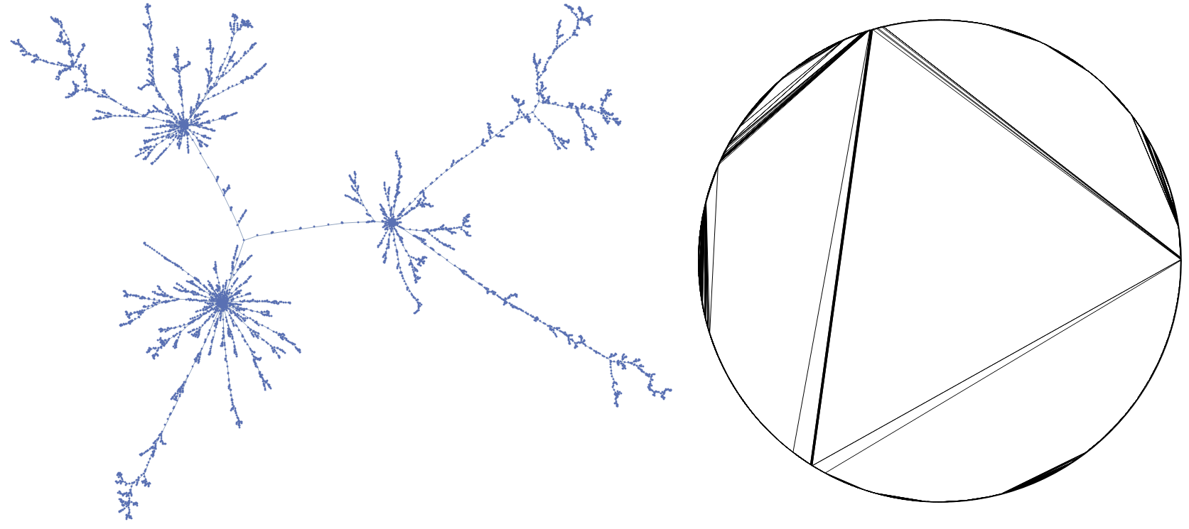
Figure 1: Simulation of an Inhomogeneous CRT $\mathcal{T}_{\theta}$ and its associated lamination $\mathbb{L}(\mathcal{T}_{\theta})$, for $\theta=(1/\sqrt{7},2/\sqrt{7},1/\sqrt{7},1/\sqrt{7},0,\ldots)$.

In the regime of possibly countably many macroscopic degrees (A.2) and (${\bf B}$), Theorem 1 characterises the possible scaling limits of this model of random trees. It is then natural to wonder whether (1) can be reinforced to hold for the stronger Gromov-Hausdorff-Prokhorov topology under the assumptions (A.1)-(A.3) and (${\bf B}$). To achieve this, one would need to prove the tightness of the sequence of discrete trees (see e.g., [5, Equation 25]), which requires precise estimates of the height of $\mathbf{t}_{n}$. However, as pointed out in [42, Section 1.2], there are cases where the maximal height of the tree can be much larger than $V_{n}/b_{n}$ and thus no general tightness result as in [20] holds.

Recently, Blanc-Renaudie [18] independently proved the result in Theorem 1; see [18, Theorem 5 (a)-(b)]. Indeed, [18, Theorem 6 (a)-(b)] shows that, under more general conditions ([18, Assumptions 1-2]), $\mathbf{t}_{n}$ converges either toward a $\mathbf{p}$-tree, or after normalization by $V_{n}/\sigma_{n}$ toward the Inhomogeneous CRT, for the Gromov-weak topology. Nevertheless, our methods are completely different. While Blanc-Renaudie introduces a new recursive construction for TGDSs based on a modified Aldous-Broder algorithm, in this work we consider a classical approach through the study of the $\L$ukasiewicz path and the height process that are relevant in their own right. On the other hand, Blanc-Renaudie [18, Theorem 7] implies, under additional tightness conditions ([18, Assumption 7]), the convergence of $\mathbf{t}_{n}$ for the Gromov–Hausdorff–Prokhorov topology. To be precise, Blanc-Renaudie provides a near-optimal upper bound for the height of $\mathbf{t}_{n}$ and uses similar estimates to control the Gromov-Hausdorff distance between $\mathbf{t}_{n}^{(q_{n})}$ and $\mathbf{t}_{n}$, for a well-chosen sequence $(q_{n},n\geq 1)$.

As we mentioned earlier, this height estimate is the ingredient missing in our approach to obtain the convergence for the Gromov–Hausdorff–Prokhorov topology. Indeed, a close inspection to the proof of [18, Lemma 25] together with [18, Lemma 14] shows [5, equation (25)], which implies that the sequence of discrete height processes of the trees $(\mathbf{t}_{n},n\geq 1)$ is tight after normalization by $V_{n}/\sigma_{n}$; see [5, proof of Theorem 20 (ii)]. In particular, under (A.1)-(A.3), (${\bf B}$) and [18, Assumption 7], the convergence of the finite-dimensional distributions (Theorem 6) and the tightness prove the weak convergence of the discrete height process toward the height process of the Inhomogeneous CRT. This implies the convergence of the contour function and thus the convergence for the Gromov–Hausdorff–Prokhorov topology; see [35, Section 1.6] and [1]. We do not include here the precise statement and proof details to avoid repeating and using the arguments introduced in [18].

Probably, the proof of the Theorem 1 could be extended to the case $\sum_{i\geq 1}\beta_{i}=\infty$. However, this broader setting brings additional technical complications that we decide not to consider in this article. For example, one would first have to define the height process of the Inhomogeneous CRT for this case, which has not yet been defined properly.

Finally, we expect that similar results also hold for forests with given degree sequence. This has only been investigated under the assumption of no macroscopic degrees by Lei [38] and Marzouk [42]. In particular, they viewed the forest as a single tree by attaching all the roots to an extra root vertex. In this framework, the limit is a different continuum tree that is encoded by a certain Brownian first-passage bridge. We believe that our approach could be used to extend this result and the results in [42] on random planar maps with a given degree sequence.

1.2 Fragmentations and laminations

Aldous, Evans and Pitman [9, 25, 45] initiated the study of fragmentation processes derived by deleting one by one the edges of tree-like structures uniformly at random. As time passes, the deletion of edges creates more and more connected components whose sequence of sizes is called the fragmentation process of the tree. Aldous, Evans and Pitman studied the case of a uniform random tree with $n$ labelled vertices and showed that the associated fragmentation process, suitably rescaled, converges to the fragmentation process of the Brownian CRT, as $n\rightarrow\infty$; see also [21, 41]. This latter is connected to the standard additive coalescent via a deterministic time-change and it is constructed by cutting down the skeleton of the Brownian CRT in a Poisson manner. Aldous and Pitman [11] (see also [25]) established a similar result in the broader context of $\mathbf{p}$-trees. They showed that this fragmentation process converges after rescaling to the fragmentation process of the limiting Inhomogeneous CRT. Recently, the authors [16] studied the case of critical Galton-Watson trees conditioned on having $n$ vertices, whose offspring distribution $\mu$ belongs to the domain of attraction of a stable law of index $\alpha\in(1,2]$ ($\alpha$-stable Galton-Watson trees). In this case, the limit is the fragmentation process of the so-called $\alpha$-stable Lévy tree constructed by cutting down its skeleton in a Poisson manner.

It turns out that the fragmentation process of a tree can be coded by a non-decreasing process of subsets of the unit disk called laminations. A lamination is a closed subset of the closed unit disk $\bar{\mathbb{D}}$ made of the union of the unit circle $\mathbb{S}^{1}$ and a set of chords that do not intersect in the open unit disk $\mathbb{D}$. A face of a lamination $L$ is a connected component of the complement of $L$ in $\bar{\mathbb{D}}$. Laminations appear for instance in topology and hyperbolic geometry, see [19] and references therein. We denote by $\mathbb{L}(\bar{\mathbb{D}})$ the set of laminations of $\bar{\mathbb{D}}$ and equip it with the usual Hausdorff topology on the compact subsets of $\bar{\mathbb{D}}$.

The idea of coding (random) tree-like structures by (random) laminations of $\bar{\mathbb{D}}$ goes back to Aldous [6, 7] in his study of a uniform triangulation of a large polygon. Since then, laminations have appeared in different contexts, as limits of discrete structures [34, 23, 47] or in the theory of random maps [37]. Roughly speaking, each chord of the lamination corresponds to an edge of the tree. Then, by adding chords one by one in the order in which they are removed, we code the fragmentation of the tree by a random process taking its values in the set of laminations $\mathbb{L}(\bar{\mathbb{D}})$. See Section 4 for a rigorous definition of this process. Furthermore, at any given time in the process, there is a one-to-one correspondence between faces of the lamination and connected components of the fragmented tree. Indeed, it can be shown that the rescaled size of a component in the fragmentation process is equal to the mass of the corresponding face, that is, $(2\pi)^{-1}$ times the fraction of its perimeter lying on the unit circle. In the case of $\alpha$-stable Galton-Watson trees, the third author proves in [47] the convergence of this lamination-valued process, toward a limiting process that can be constructed directly from the corresponding $\alpha$-stable Lévy tree and encodes its fragmentation process.

A natural way of extending the previous investigations is to study the asymptotic behaviour of the fragmentation process and the lamination-valued process derived by cutting-down a rooted plane tree, and in particular a tree with given degree sequence. This is the second goal of this paper. To present the main result of this section, we need some notation and background that some readers may not be familiar with. We refer to Section 4 for proper definitions. Let $(\mathbb{L}_{t}(\tau),t\geq 0)$ be the lamination-valued process associated to $\tau$ (that is, for all $t\geq 0$, $\mathbb{L}_{t}(\tau)$ is obtained by removing the first $\lfloor t\rfloor\wedge(\zeta(\tau)-1)$ edges from $\tau$); see Definition 1. Let $\mathbf{D}(I,\mathbb{M})$ be the space of càdlàg functions (that is, right-continuous with left limits) from an interval $I\subseteq\mathbb{R}_{+}$ to a separable, complete metric space $\mathbb{M}$. We equip $\mathbf{D}(I,\mathbb{M})$ with the $J_{1}$ Skorohod topology; see e.g.  [17, Chapter 3] or [31, Chapter VI] for details on this space. We denote by $\mathcal{T}=(\mathcal{T},r,\rho,\mu)$ a continuum tree, that is, $(\mathcal{T},r)$ is a metric space, $\rho$ is a distinguished element of $\mathcal{T}$ called the root and $\mu$ is a probability measure on the set of leaves of $\mathcal{T}$; see Definition 5. As in the case of finite trees, it is possible to define from $\mathcal{T}$ a lamination-valued process $(\mathbb{L}_{t}(\mathcal{T}),t\geq 0)$ obtained by cutting $\mathcal{T}$ in a Poissonian way and associating to each cutpoint a chord in the disk; see Definition 7. For $n\geq 1$, we let $\tau_{n}$ be a rooted plane tree and we see it as a rooted metric measure space $(\tau_{n},r_{n}^{\text{gr}},\emptyset_{n},\mu_{n})$, i.e., $\tau_{n}$ is identified as its set of $\zeta(\tau_{n})$ vertices, $r_{n}^{\text{gr}}$ is the graph distance on $\tau_{n}$, $\emptyset_{n}$ is the root of $\tau_{n}$ and $\mu_{n}$ is the uniform measure on the set of vertices of $\tau_{n}$. The following result, which in particular can be applied to trees with given degree sequence, states the equivalence of the Gromov-weak convergence of a sequence of plane trees and the convergence its associated lamination-valued processes.

Theorem 2.

Let $(\tau_{n},n\geq 1)$ be a sequence of rooted plane trees, $\mathcal{T}$ be a continuum tree and $(a_{n},n\geq 1)$ be a sequence of non-negative real numbers satisfying $a_{n}\rightarrow\infty$ and $\zeta(\tau_{n})/a_{n}\rightarrow\infty$, as $n\rightarrow\infty$. Then, the following assertions are equivalent:

1. The following holds in $\mathbf{D}(\mathbb{R}_{+},\mathbb{L}(\bar{\mathbb{D}}))$:

   $$(\mathbb{L}_{ta_{n}}(\tau_{n}),t\geq 0)\xrightarrow[]{d}(\mathbb{L}_{t}(\mathcal{T}),t\geq 0),\hskip 8.53581pt\text{as}\hskip 5.69054ptn\rightarrow\infty,\hskip 5.69054pt.$$

2. $\displaystyle\left(\tau_{n},\frac{a_{n}}{\zeta(\tau_{n})}r_{n}^{\rm gr},\emptyset_{n},\mu_{n}\right)\rightarrow(\mathcal{T},r,\rho,\mu)$, as $n\rightarrow\infty$, for the Gromov-weak topology.

To prove Theorem 2, we develop a general approach that is based on the notion of reduced laminations that may be of independent interest. These reduced laminations are constructed considering reduced trees obtained by sampling only a finite number of vertices in the tree. In particular, the more vertices are sampled, the closer one is to the lamination-valued process associated with the entire tree.

Theorem 1 and Theorem 2 immediately entail the following result about the lamination-valued process associated with the fragmentation of a tree with given degree sequence $\mathbf{t}_{n}$.

Corollary 1.

Suppose that $\mathbf{s}_{n}$ satisfies (A.1)-(A.3) and (${\bf B}$). Let $\mathcal{T}_{\theta}$ be an Inhomogeneous CRT with parameter set $\theta=(\theta_{0},\theta_{1},\dots)$ given by $\theta_{0}=\sigma$ and $\theta_{i}=\beta_{i}$, for $i\geq 1$. Then, jointly with the convergence of Theorem 1, we have that

$$(\mathbb{L}_{tb_{n}}(\mathbf{t}_{n}),t\geq 0)\xrightarrow[]{d}(\mathbb{L}_{t}(\mathcal{T}_{\theta}),t\geq 0),\hskip 8.53581pt\text{as}\hskip 5.69054ptn\rightarrow\infty,\hskip 5.69054pt\text{in}\hskip 5.69054pt\mathbf{D}(\mathbb{R}_{+},\mathbb{L}(\bar{\mathbb{D}})).$$

In Figure 1, one can see a simulation of $\mathbb{L}_{\infty}(\mathcal{T}_{\theta})\coloneqq\lim_{t\rightarrow\infty}\mathbb{L}_{t}(\mathcal{T}_{\theta})$, for a given parameter set $\theta$. Indeed, Theorem 2 and [18, Theorem 5 (b)] imply the convergence of lamination-valued processes associated even to trees with given degree sequence $\mathbf{s}_{n}$ satisfying [18, Assumption 2]. In this case, the limit is the lamination-valued process associated to an Inhomogeneous CRT. Moreover, by the well-known convergence of suitably rescaled $\mathbf{p}$-trees ([11, 22, 18]), one can apply Theorem 2 to establish the convergence of the corresponding lamination-valued processes. Theorem 2 also provides another proof to [47, Theorems 1.2 and 3.3], in the case of $\alpha$-stable Galton-Watson trees.

Theorem 2 (or Corollary 1) does not a priori imply the convergence, after a proper rescaling, of the underlying fragmentation process associated to a tree with given degree sequence $\mathbf{t}_{n}$. However, this convergence can be independently obtained without relying on the scaling limit of $\mathbf{t}_{n}$. For convenience, let us define a slightly different version of the fragmentation process, where edges are removed at i.i.d. times and not at integer times. It turns out that, asymptotically, these two fragmentation processes have the same behaviour. Equip the edges of $\mathbf{t}_{n}$ with i.i.d. random weights uniform on $[0,1]$ (independent of $\mathbf{t}_{n}$). For $u\in[0,1]$, consider the forest $\mathbf{f}_{n}(u)$ of connected components created by keeping the edges of $\mathbf{t}_{n}$ with weight smaller than or equal to $u$ and by discarding the others. Let $\mathbf{F}_{n}=(\mathbf{F}_{n}(u),u\in[0,1])$ be the process given by

$$\mathbf{F}_{n}(u)=(F_{n,1}(1-u),F_{n,2}(1-u),\dots),\hskip 8.53581pt\text{for}\hskip 5.69054ptu\in[0,1],$$

the sequence of sizes (number of vertices) of the connected components of the forest $\mathbf{f}_{n}(1-u)$, ranked in non-increasing order. We strategically view the sequence of sizes as an infinite sequence, by completing it with an infinite number of zero terms. Plainly as time passes more and more connected components are created, and thus, the process $\mathbf{F}_{n}$ evolves as a fragmentation process. Note also that $\mathbf{F}_{n}(0)=(V_{n},0,0,\dots)$ and that $\mathbf{F}_{n}(1)=(1,1,\dots,1,0,0,\dots)$ are infinite sequences (where the first $V_{n}$ terms are $1$’s in $\mathbf{F}_{n}(1)$). We call $\mathbf{F}_{n}$ the dynamical fragmentation process of $\mathbf{t}_{n}$. Consider the infinite ordered set

$$\bm{\Delta}\coloneqq\Big{\{}\mathbf{x}=(x_{1},x_{2},\dots):x_{1}\geq x_{2}\geq\cdots\geq 0\hskip 5.69054pt\text{and}\hskip 5.69054pt\sum_{i=1}^{\infty}x_{i}<\infty\Big{\}},$$

endowed with the $\ell^{1}$-norm, $\|\mathbf{x}\|_{1}=\sum_{i=1}^{\infty}|x_{i}|$ for $\mathbf{x}\in\bm{\Delta}$.

Theorem 3.

Suppose that $\mathbf{s}_{n}$ satisfies (A.1)-(A.3) and

1. Unbounded variation. Either $\sigma^{2}>0$ or $\sum_{i\geq 1}\beta_{i}=\infty$.

Then, there exists a process $(\mathbf{F}(t),t\geq 0)$ such that

$$\left(\frac{1}{V_{n}}\mathbf{F}_{n}\left(t\frac{b_{n}}{V_{n}}\right),t\geq 0\right)\xrightarrow[]{d}(\mathbf{F}(t),t\geq 0),\hskip 8.53581pt\text{as}\hskip 5.69054ptn\rightarrow\infty,\hskip 5.69054pt\text{in}\hskip 5.69054pt\mathbf{D}(\mathbb{R}_{+},\bm{\Delta}).$$

The limiting process $(\mathbf{F}(t),t\geq 0)$ corresponds precisely to the fragmentation process constructed by Bertoin [14, 15] via partitions of the unit interval induced by certain bridges with exchangeable increments. For a precise construction, we refer to Section 5 in which we actually prove a more general result about the convergence of the fragmentation process of rooted plane trees. On the other hand, if $\sigma^{2}+\sum_{i\geq 1}\beta_{i}^{2}=1$ then $(\mathbf{F}(t),t\geq 0)$ coincides with the fragmentation process of the Inhomogeneous CRT, with parameter set $\theta=(\theta_{0},\theta_{1},\dots)$ given by $\theta_{0}=\sigma$ and $\theta_{i}=\beta_{i}$, for $i\geq 1$; see [11].

Finally, as a consequence of Theorem 3, we relate the sequence of masses of the faces of $(\mathbb{L}_{t}(\mathcal{T}_{\theta}),t\geq 0)$ with the fragmentation process $(\mathbf{F}(t),t\geq 0)$. For any lamination $L\in\mathbb{L}(\bar{\mathbb{D}})$, let $\mathbb{M}{\rm ass}[L]$ denote the sequence of the masses of its faces, sorted in non-increasing order.

Corollary 2.

Suppose that $\mathbf{s}_{n}$ satisfies (A.1)-(A.4) with $\sigma^{2}+\sum_{i\geq 1}\beta_{i}^{2}=1$. Then,

$$(\mathbb{M}{\rm ass}[\mathbb{L}_{tb_{n}}(\mathbf{t}_{n})],t\geq 0)\xrightarrow[]{d}\left(\mathbf{F}(t),t\geq 0\right),\hskip 8.53581pt\text{as}\hskip 5.69054ptn\rightarrow\infty,\hskip 5.69054pt\text{in}\hskip 5.69054pt\mathbf{D}(\mathbb{R}_{+},\bm{\Delta}).$$

Furthermore, $(\mathbb{M}{\rm ass}[\mathbb{L}_{t}(\mathcal{T}_{\theta})],t\geq 0)=\left(\mathbf{F}(t),t\geq 0\right)$ almost surely, where $\mathcal{T}_{\theta}$ is an Inhomogeneous CRT with parameter set $\theta=(\theta_{0},\theta_{1},\dots)$ given by $\theta_{0}=\sigma$, $\theta_{i}=\beta_{i}$, for $i\geq 1$.

Let us finish with some remarks on the assumptions that we make on the degree sequences. The hypotheses size (A.1), hubs (A.2), degree variance (A.3) and unbounded variation (A.4) are exactly those made in [13] to study the profile of a TGDS. They are necessary to apply the characterization and convergence results for exchangeable increments processes of [32] that are crucial to understand the shape of a TGDS via its $\L$ukasiewicz path and up to some extent its height process. Let us also point out that the hypotheses (A.1)-(A.4) are included in [18, Assumption 2].

1.3 Organization

In Section 2, we first recall the definition of rooted plane trees and their encoding by paths. In Section 3, we prove Theorem 1 by studying the behaviour of a modified version of the $\L$ukasiewicz paths associated with trees with given degree sequence. Section 4 is devoted to the study of lamination-valued processes of discrete trees and continuum trees; we prove in particular Theorem 2 and Corollary 2 about the convergence of the geometric representation of trees by laminations. Finally, in Section 5, we prove Theorem 3, showing the convergence of the associated fragmentation processes.

Notation.

For $f\in\mathbf{D}(I,\mathbb{R})$, we denote by $f(t)$ the value of $f$ at $t\in I$, by $f(t-)$ its left-hand limit at time $t$ (with the convention $f(0-)=f(0)$ if $0\in I$) and by $\Delta f(t)=f(t)-f(t-)$ the size of the jump (if any) at $t$.

We write $\xrightarrow[]{d}$, $\xrightarrow[]{\mathbb{P}}$ and $\xrightarrow[]{a.s.}$ to denote convergence in distribution, probability and almost surely, respectively.

Let $(A_{n},n\geq 1)$ and $(B_{n},n\geq 1)$ be two sequences of real random variables such that $B_{n}>0$, for all $n\geq 1$. We say that $A_{n}=o(B_{n})$ in probability if $\lim_{n\rightarrow\infty}|A_{n}|/B_{n}=0$ in probability.

2 Plane trees and their encoding paths

We provide here some background on finite rooted trees and recall how they can be coded by different integer-valued paths.

Following [44], let $\mathbb{N}=\{1,2,\dots\}$ be the set of positive integers, set $\mathbb{N}^{0}=\{\emptyset\}$ and consider the set of labels $\mathbb{U}=\bigcup_{n\geq 0}\mathbb{N}^{n}$. An element $u\in\mathbb{U}$ is a sequence $u=(u_{1},\dots,u_{n})$ of positive integers. If $v=(v_{1},\dots,v_{m})\in\mathbb{U}$, we let $uv=(u_{1},\dots,u_{n},v_{1},\dots,v_{m})\in\mathbb{U}$ be the concatenation of $u$ and $v$. By a slight abuse of notation, if $z\in\mathbb{N}$, we let $uz=(u_{1},\dots,u_{n},z)$. A rooted plane tree is a non-empty, finite subset $\tau\subset\mathbb{U}$ such that: (i) $\emptyset\in\tau$; (ii) if $v\in\tau$ and $v=uz$ for some $z\in\mathbb{N}$, then $u\in\tau$; (iii) if $u\in\tau$, then there exists an integer $k_{u}\geq 0$ such that $ui\in\tau$ if and only if $1\leq i\leq k_{u}$. We view each vertex $u$ of $\tau$ as an individual of a population whose genealogical tree is $\tau$. The vertex $\emptyset$ is called the root of the tree. For every $u=(u_{1},\dots,u_{n})\in\tau$, the vertex $pr(u)=(u_{1},\dots,u_{n-1})$ is its parent, $k_{u}$ represents the number of children of $u$ (if $k_{u}=0$, then $u$ is called a leaf, otherwise, $u$ is called an internal vertex), and $|u|=n$ represents the length (or generation, or height) of $u$. We let $\chi_{u}\in\{1,\dots,k_{pr(u)}\}$ be the only index such that $u=pr(u)\chi_{u}$, which is the relative position of $u$ amongst its siblings. The total progeny (or size) of $\tau$ will be denoted by $\zeta(\tau)=\text{Card}(\tau)$ (i.e., the number of vertices of $\tau$). In the following, by tree, we will always mean a rooted plane tree and we denote the set of all trees by $\mathbb{T}$. By a slight abuse, we sometimes consider a tree $\tau$ as a metric space, by drawing an edge of length $1$ between each non-root vertex $u$ and its parent $pr(u)$.

We will use three different orderings of the vertices of a tree $\tau\in\mathbb{T}$:

• Lexicographical ordering. Given $v,w\in\tau$, we write $v\prec_{\text{lex}}w$ if there exists $z\in\tau$ such that $v=z(v_{1},\dots,v_{n})$, $w=z(w_{1},\dots,w_{m})$ and $v_{1}<w_{1}$.

• Reverse-lexicographical ordering. Given $v,w\in\tau$, we write $v\prec_{\text{rev}}w$ if $w\prec_{\text{lex}}v$.

• Prim ordering. Let $\textbf{edge}(\tau)$ be the set of edges of $\tau$ and consider a sequence of distinct and positive weights $\mathbf{w}=(w_{e}:e\in\textbf{edge}(\tau))$ (i.e., each edge $e$ of $\tau$ is marked with a different and positive weight $w_{e}$). Given two distinct vertices $u,v\in\tau$, we write $\{u,v\}$ for the edge connecting $u$ and $v$ in $\tau$ - if it exists. Let us describe the Prim order $\prec_{\text{prim}}$ of the vertices in $\tau$, that is, $\emptyset=u(0)\prec_{\text{prim}}u(1)\prec_{\text{prim}}\dots\prec_{\text{prim}}u(\zeta(\tau)-1)$. First set $u(0)=\emptyset$ and $V_{1}=\{u(0)\}$. Suppose that for some $1\leq i\leq\zeta(\tau)-1$, the vertices $u(0),\dots,u(i-1)$ have been defined. We will use the notation $V_{i}$ for the set $\{u(0),\dots,u(i-1)\}$, for $0\leq i\leq\zeta(\tau)-1$. Consider the minimum of the set of weights $\{w_{\{u,v\}}:u\in V_{i},v\not\in V_{i}\}$ of the edges between a vertex of $V_{i}$ and another outside of $V_{i}$. Since all the weights are distinct, this minimum is reached at a unique edge $\{\tilde{u},\tilde{v}\}$ where $\tilde{u}\in V_{i}$ and $\tilde{v}\not\in V_{i}$. Then set $u(i)=\tilde{v}$. This iterative procedure completely determines the Prim order $\prec_{\text{prim}}$.

$\L$ukasiewicz path, reverse-$\L$ukasiewicz path and Prim path.

Fix $\tau\in\mathbb{T}$, and for $\ast\in\{{\rm lex},{\rm rev},{\rm prim}\}$, associate to the ordering $\emptyset=u(0)\prec_{\ast}u(1)\prec_{\ast}\dots\prec_{\ast}u(\zeta(\tau)-1)$ of its vertices a path $W_{\tau}^{\ast}=(W_{\tau}^{\ast}(i),0\leq i\leq\zeta(\tau))$, by letting $W_{\tau}^{\ast}(0)=0$ and for $0\leq i\leq\zeta(\tau)-1$, $W_{\tau}^{\ast}(i+1)=W_{\tau}^{\ast}(i)+k_{u(i)}-1$. Observe that $W_{\tau}^{\ast}(i+1)-W_{\tau}^{\ast}(i)=k_{u(i)}-1\geq-1$ for every $0\leq i\leq\zeta(\tau)-1$, with equality if and only if $u(i)$ is a leaf of $\tau$. Note also that $W_{\tau}^{\ast}(i)\geq 0$ for every $0\leq i\leq\zeta(\tau)-1$, but $W_{\tau}^{\ast}(\zeta(\tau))=-1$. We shall think of such a path as the step function on $[0,\zeta(\tau)]$ given by $s\mapsto W_{\tau}^{\ast}(\lfloor s\rfloor)$. The path $W^{\text{lex}}_{\tau}$ is usually called the $\L$ukasiewicz path of $\tau$ and we will refer to $W^{\text{rev}}_{\tau}$ and $W^{\text{prim}}_{\tau}$ as the reverse-$\L$ukasiewicz path and the Prim path of $\tau$, respectively.

For $u,v\in\tau$, we denote by $\llbracket u,v\rrbracket$ the unique geodesic path between $u$ and $v$ in $\tau$, and $\llbracket u,v\llbracket=\llbracket u,v\rrbracket\backslash\{v\}$. In particular, we write $\llbracket\varnothing,u\llbracket$ for the ancestral line or branch of $u$. For $u\in\tau$, let us denote by ${\rm L}(u)$ and ${\rm R}(u)$ respectively the number of vertices whose parent is a strict ancestor of $u$ and which lie strictly to the left (respectively to the right) of the ancestral line $\llbracket\emptyset,u\llbracket$. Then, we set ${\rm LR}(u)={\rm L}(u)+{\rm R}(u)$, the total number individuals branching-off the ancestral line of $u$. In particular, let $\emptyset=u(0)\prec_{\text{lex}}u(1)\prec_{\text{lex}}\dots\prec_{\text{lex}}u(\zeta(\tau)-1)$ be the sequence of vertices of $\tau$ in lexicographical order. Then, one readily sees that

$${\rm R}(u(i))=W^{\text{lex}}_{\tau}(i),\hskip 11.38109pt\text{for}\hskip 5.69054pt0\leq i\leq\zeta(\tau)-1.$$ (2)

Similarly, if $\emptyset=u(0)\prec_{\text{rev}}u(1)\prec_{\text{rev}}\dots\prec_{\text{rev}}u(\zeta(\tau)-1)$ are listed in reverse-lexicographical order, then

$${\rm L}(u(i))=W^{\text{rev}}_{\tau}(i),\hskip 11.38109pt\text{for}\hskip 5.69054pt0\leq i\leq\zeta(\tau)-1.$$ (3)

Height process.

Let $\emptyset=u(0)\prec_{\text{lex}}u(1)\prec_{\text{lex}}\dots\prec_{\text{lex}}u(\zeta(\tau)-1)$ be the sequence of vertices of $\tau\in\mathbb{T}$ in lexicographical order. The height process $H_{\tau}=(H_{\tau}(i):0\leq i\leq\zeta(\tau))$ of $\tau$ is defined by letting $H_{\tau}(i)=|u(i)|$, for every $i\in\{0,\dots,\zeta(\tau)-1\}$, and $H_{\tau}(\zeta(\tau))=0$. We sometimes think of $H_{\tau}$ as a continuous function on $[0,\zeta(\tau)]$, obtained by linear interpolation.

Contour function.

The contour function $C_{\tau}=(C_{\tau}(t),s\in[0,2\zeta(\tau)])$ of $\tau\in\mathbb{T}$ is defined as follows. Imagine a particle exploring $\tau$ from left to right at unit speed, going backwards when it reaches a leaf. For all $s\in[0,2\zeta(\tau)-2]$, let $C_{\tau}(s)$ be the distance from the particle to the root $\emptyset$ at time $s$. By convention, we set $C_{\tau}(s)=0$ for $s\in[2\zeta(\tau)-2,2\zeta(\tau)]$. In particular, $C_{\tau}$ is continuous and $C_{\tau}(0)=C_{\tau}(2\zeta(\tau))=0$.

3 Convergence of the trees with given degrees

In this section, we prove Theorem 1 which states the convergence of trees with a given degree sequence toward the Inhomogeneous CRT. In Section 3.1, we first recall the definition of the exploration process that encodes the Inhomogeneous CRT. In Section 3.2, we introduce the discrete version of the above exploration process, the so-called modified $\L$ukasiewicz path, which encodes a TGDS. We then prove that this modified $\L$ukasiewicz path, suitably rescaled, converges to the exploration process of the Inhomogeneous CRT, which implies Theorem 1. Finally, in Section 3.3, we consider a specific case in which we can prove the convergence of the trees for the Gromov-Hausdorff-Prokhorov topology.

3.1 The exploration process of the Inhomogeneous CRT

Let us start with some definitions. A bridge with exchangeable increments (abridged EI process) is a continuous-time stochastic process $X^{\rm bg}=(X^{\rm bg}(t),t\in[0,1])$ with paths in $\mathbf{D}([0,1],\mathbb{R})$ and of the form

$$X^{\rm bg}(t)=\sigma B^{\rm bg}(t)+\sum_{i=1}^{\infty}\beta_{i}(\mathbf{1}_{\{U_{i}\leq t\}}-t),\hskip 11.38109ptt\in[0,1],$$

where $B^{\rm bg}=(B^{\rm bg}(t),t\in[0,1])$ is a Brownian bridge on $[0,1]$, $(U_{i},i\geq 1)$ are i.i.d. random variables with uniform law on $[0,1]$ independent of $B^{\rm bg}$, and $\sigma\in\mathbb{R}_{+}$, $\beta_{1}\geq\beta_{2}\geq\cdots\geq 0$ are constants such that $\sum_{i\geq 1}\beta_{i}^{2}<\infty$. We say that $X^{\rm bg}$ is an EI process with parameters $(\sigma,(\beta_{i},i\geq 1))$.

The so-called Vervaat transform (or Vervaat excursion) was introduced by Takács [46] and used by Vervaat [48] to change a bridge-type process with paths in $\mathbf{D}([0,1],\mathbb{R})$ into an excursion-type process, i.e., a non-negative process that is equal to $0$ at times $0$ and $1$. More precisely, let $X=(X(t),t\in[0,1])$ be a stochastic process with paths in $\mathbf{D}([0,1],\mathbb{R})$ such that $X(0)=X(1)=X(1-)=0$. Assume that $X$ reaches its infimum value uniquely and continuously at $\rho$. The Vervaat transform of $X$ is the stochastic process $V(X)=(V(t),t\in[0,1])$ with paths in $\mathbf{D}([0,1],\mathbb{R})$, defined by $V(t)=X(\{t+\rho\})-X(\rho)$, for $t\in[0,1]$, where $\{s\}$ is the fractional part of $s$. In particular, $V(X)$ is a non-negative process on $[0,1]$.

Through this manuscript, unless otherwise specified, we always consider EI processes $X^{\rm bg}$ with parameters $(\sigma,(\beta_{i},i\geq 1))$ satisfying (A.4), i.e. either $\sigma^{2}>0$ or $\sum_{i\geq 1}\beta_{i}=\infty$. This is a necessary and sufficient condition for $X^{\rm bg}$ to have paths of infinite variation. More importantly, by [33] or [15, Proof of Lemma 6], it is well-known that under this condition $X^{\rm bg}$ almost surely achieves its infimum at a unique time $\rho$ and continuously. Then, we let $X^{\rm exc}=(X^{\rm exc}(t),t\in[0,1])$ be the excursion-type process associated to $X^{\rm bg}$ via its Vervaat transform.

The excursion process $X^{\rm exc}$ is not necessarily continuous. However, following [8, Section 2], one can also associate to $X^{\rm bg}$ a continuous excursion process $H^{\rm exc}$. For all $i\geq 1$, write $t_{i}=\{U_{i}-\rho\}$ (the fractional part of $U_{i}-\rho$) for the location of the jump with size $\beta_{i}$ in $X^{\rm exc}$. For each $i\geq 1$ such that $\beta_{i}>0$, write $T_{i}=\inf\{t\in(t_{i},1]:X^{\rm exc}(t)=X^{\rm exc}(t_{i}-)\}$, which exists since the process $X^{\rm exc}$ has no negative jumps and goes back to $0$ at time $1$. In particular, all $t_{i}$’s and $T_{i}$’s are distinct almost surely. For $u\in[0,1]$ and $i\geq 1$ such that $\beta_{i}>0$, let $R_{i}=(R_{i}(u),u\in[0,1])$ be the process defined by

$$R_{i}(u)=\left\{\begin{array}[]{lcl}\inf_{t_{i}\leq s\leq u}X^{\rm exc}(s)-X^{\rm exc}(t_{i}-)&\mbox{ if }&u\in[t_{i},T_{i}],\\ 0&&\mbox{otherwise}.\\ \end{array}\right.$$ (6)

If $\beta_{i}=0$ then let $R_{i}$ be the null process on $[0,1]$. Define the process $H^{\rm exc}=(H^{\rm exc}(u),u\in[0,1])$ by

$$H^{\rm exc}(u)=X^{\rm exc}(u)-\sum_{i\geq 1}R_{i}(u),\hskip 11.38109pt\text{for}\hskip 5.69054ptu\in[0,1].$$

As explained in [8, Section 2], $H^{\rm exc}$ is a well-defined continuous excursion-type process. Furthermore, Aldous, Miermont and Pitman [8, Theorem 1] also showed that $H^{\rm exc}$ can be used to define an exploration process that encodes the structure of an Inhomogeneous CRT with parameter set $\theta=(\theta_{0},\theta_{1},\dots)$ satisfying $\theta_{1}\geq\theta_{2}\geq\cdots\geq 0$, $\theta_{0}>0$, $\sum_{i\geq 0}\theta_{i}^{2}=1$ and $\sum_{i\geq 1}\theta_{i}<\infty$.

3.2 The modified $\L$ukasiewicz path

For $n\in\mathbb{N}$, let $\mathbf{s}_{n}$ be a degree sequence, $\mathbf{t}_{n}$ be a tree sampled uniformly at random in $\mathbb{T}_{\mathbf{s}_{n}}$ and $W_{n}^{\rm lex}=(W_{n}^{\rm lex}(V_{n}u),u\in[0,1])$ denote its time-rescaled $\L$ukasiewicz path; recall that $V_{n}$ denotes the number of vertices in $\mathbf{t}_{n}$.

Theorem 4.

Suppose that $\mathbf{s}_{n}$ satisfies (A.1)-(A.4). Then,

$$(b_{n}^{-1}W_{n}^{\rm lex}(V_{n}u),u\in[0,1])\xrightarrow[]{d}(X^{\rm exc}(u),u\in[0,1]),\hskip 8.53581pt\text{as}\hskip 5.69054ptn\rightarrow\infty,\hskip 5.69054pt\text{in}\hskip 5.69054pt\mathbf{D}([0,1],\mathbb{R}).$$

Proof.

It follows as in the proof of [13, Proposition 1], where a similar result is proved for the so-called breadth-first walk of $\mathbf{t}_{n}$, which has the same law as its $\L$ukasiewicz path. ∎

We now describe a modification of $W^{\text{lex}}_{n}$ from which we construct the discrete analogue of $H^{\rm exc}$. For $1\leq i\leq V_{n}$, write $t_{i}^{n}$ for the location of the jump with size $d^{n}(i)-1$ in $W^{\text{lex}}_{n}$. In the case where there are $1\leq i<j$ such that $\beta_{i}=\beta_{k}>0$, for $k=i,\dots,j$ (and $\beta_{k}\neq\beta_{i}$ otherwise), we sort them from left to right by letting $t_{k}^{n}=t_{(k-i+1)}^{n}$, where $t_{(k-i+1)}^{n}$ is the $(k-i+1)$-th smallest element of the set $\{t_{i}^{n},\dots,t_{j}^{n}\}$. We also set $T_{i}^{n}=\inf\{u\in(t_{i}^{n},1]:W^{\text{lex}}_{n}(V_{n}u)-W^{\text{lex}}_{n}(V_{n}t_{i}^{n}-)=-1\}$. Let $R_{i}^{n}=(R_{i}^{n}(u),u\in[0,1])$ be the process given by

$$R_{i}^{n}(u)=\left\{\begin{array}[]{lcl}\inf_{t_{i}^{n}\leq s\leq u}W^{\text{lex}}_{n}(V_{n}s)-W^{\text{lex}}_{n}(V_{n}t_{i}^{n}-)&\mbox{ if }&u\in[t_{i}^{n},T_{i}^{n}],\\ 0&\mbox{otherwise}.&\\ \end{array}\right.$$

Consider a sequence $(I_{n},n\geq 1)$ of non-negative numbers such that $I_{n}\uparrow\infty$, as $n\rightarrow\infty$. Then, define the modified $\L$ukasiewicz path $G_{n}=(G_{n}(V_{n}u),u\in[0,1])$ of $\mathbf{t}_{n}$ by letting

$$G_{n}(V_{n}u)=\left\{\begin{array}[]{lcl}W^{\rm lex}_{n}(V_{n}u)&\mbox{ if }&\beta_{1}=0,\\ W^{\rm lex}_{n}(V_{n}u)-\sum_{i=1}^{I_{n}}R_{i}^{n}(u)&\mbox{otherwise.}&\\ \end{array}\right.$$

We henceforth denote by $(H^{\rm exc}(u),u\in[0,1])$ the continuous excursion-type process associated to an EI process with parameters $(\sigma,(\beta_{i},i\geq 1))$ satisfying (${\bf B}$), i.e., $\sigma^{2}>0$, $\sum_{i\geq 1}\beta_{i}<\infty$ and $\sigma^{2}+\sum_{i\geq 1}\beta_{i}^{2}=1$; see Section 3.1. Let $\mathbf{C}([0,1],\mathbb{R})$ be the space of real-valued continuous functions on $[0,1]$ equipped with the uniform topology.

Theorem 5.

Suppose that $\mathbf{s}_{n}$ satisfies (A.1)-(A.3) and (${\bf B}$). Then, there exists a non-decreasing sequence $(I_{n},n\geq 1)$ of non-negative numbers such that

$$\lim_{n\rightarrow\infty}I_{n}/b_{n}=0,\hskip 8.53581pt\lim_{n\rightarrow\infty}I_{n}=\infty\hskip 8.53581pt\text{and}\hskip 8.53581pt\lim_{I\rightarrow\infty}\limsup_{n\rightarrow\infty}b_{n}^{-1}\sum_{I\leq i\leq I_{n}}d^{n}(i)=0. {\bf S}$$ ()

Moreover, for $G_{n}$ constructed from such a sequence $(I_{n},n\geq 1)$, we have that

$$\left(b_{n}^{-1}G_{n}(V_{n}u),b_{n}^{-1}W^{{\rm lex}}_{n}(V_{n}u):u\in[0,1]\right)\xrightarrow[]{d}(H^{\rm exc}(u),X^{\rm exc}(u):u\in[0,1]),\hskip 8.53581pt\text{as}\hskip 5.69054ptn\rightarrow\infty,$$

in $\mathbf{D}([0,1],\mathbb{R})\otimes\mathbf{D}([0,1],\mathbb{R})$. In particular,$(b_{n}^{-1}G_{n}(V_{n}u),u\in[0,1])$ converges to $H^{\rm exc}$ uniformly on $[0,1]$.

Proof.

First, we prove the existence of a non-decreasing sequence $(I_{n},n\geq 1)$ that satisfies (${\bf S}$). Since $\sum_{i\geq 1}\beta_{i}<\infty$ by (${\bf B}$), there exists an increasing sequence $(j_{k},k\geq 1)$ such that $\sum_{i\geq j_{k}}\beta_{i}<k^{-2}$, for every $k\geq 1$. Now, by (${\bf B}$) again, for every fixed $k\geq 1$ and $j\geq j_{k}$, we have that $b_{n}^{-1}\sum_{j_{k}\leq i\leq j}d^{n}(i)<k^{-2}$ for $n$ large enough. Hence, there exists $N(k,j)$ such that for any $n\geq N(k,j)$ we have that $b_{n}^{-1}\sum_{j_{k}\leq i\leq j}d^{n}(i)<k^{-2}$. So, for every fixed $k\geq 1$, there exists a non-decreasing sequence $(J_{k,n},n\geq 1)$ such that $\lim_{n\rightarrow\infty}J_{k,n}=\infty$ and for $n$ large enough (depending on $k$), $b_{n}^{-1}\sum_{j_{k}\leq i\leq J_{k,n}}d^{n}(i)<k^{-2}$. Finally, the sequence $(I_{n},n\geq 1)$ defined by $I_{1}=j_{1}$, $I_{n}=J_{1,n}$ until $J_{1,n}>j_{2}$, $I_{n}=J_{2,n}$ until $J_{2,n}\geq j_{3}$, and so on, satisfies (${\bf S}$); it is clear that we can construct $(I_{n},n\geq 1)$ such that $I_{n}/b_{n}\rightarrow 0$, as $n\rightarrow\infty$.

We now prove the second claim of Theorem 5. Recall that the modified $\L$ukasiewicz path $G_{n}$ is defined with $(I_{n},n\geq 1)$ such that (${\bf S}$) is fulfilled. If $\beta_{1}=0$, our claim follows from Theorem 4. Suppose now that $\beta_{1}>0$. By the Skorohod representation theorem, we can and will assume that the convergence of Theorem 4 holds almost surely. Consider $I\geq 1$ such that $\beta_{I}>\beta_{I+1}$. For $1\leq i\leq I$, recall that $t_{i}$ denotes the location of the jump with size $\beta_{i}$ of $X^{{\rm exc}}$ and that $T_{i}=\inf\{t\in(t_{i},1]:X^{\rm exc}(t)=X^{\rm exc}(t_{i}-)\}$. Recall also that $R_{i}=(R_{i}(u),u\in[0,1])$ denotes the process defined in (6). We claim that almost surely, for each $1\leq i\leq I$,

• $\lim_{n\rightarrow\infty}t_{i}^{n}=t_{i}$,

• $\lim_{n\rightarrow\infty}T_{i}^{n}=T_{i}$ and

• $\left(b_{n}^{-1}R_{n}^{i}(u),u\in[0,1]\right)\rightarrow(R_{i}(u),u\in[0,1])$, as $n\rightarrow\infty$, in $\mathbf{D}([0,1],\mathbb{R})$.

Assume that this holds, and let $J(X^{{\rm exc}})=\{u\in[0,1]:\Delta X^{{\rm exc}}(u)=0\}$ be the set of continuity points of $X^{{\rm exc}}$. For $1\leq i\leq I$, the set of continuity points of $R_{i}$ is $[0,1]\setminus\{t_{i}\}$. Then, it follows from [31, Proposition 2.1 in Chapter VI] that for each $u\in J(X^{{\rm exc}})$ there is a sequence $(u_{n},n\geq 0)$ such that $\lim_{n\rightarrow\infty}u_{n}=u$ and

$$\lim_{n\rightarrow\infty}b_{n}^{-1}\Delta R_{n}^{i}(u_{n})=\Delta R_{i}(u)=0=\Delta X^{{\rm exc}}(u)=\lim_{n\rightarrow\infty}b_{n}^{-1}\Delta W^{{\rm lex}}_{n}(V_{n}u_{n}).$$

On the other hand, for $1\leq i\leq I$, it follows from (A.2) that

$$\lim_{n\rightarrow\infty}b_{n}^{-1}\Delta R_{n}^{i}(t_{i}^{n})=\Delta R_{i}(t_{i})=\beta_{i}=\Delta X^{{\rm exc}}(t_{i})=\lim_{n\rightarrow\infty}b_{n}^{-1}\Delta W^{{\rm lex}}_{n}(V_{n}t_{i}^{n}).$$

Moreover, for $1\leq j\leq I$ such that $j\neq i$, (A.2) also implies that

$$\lim_{n\rightarrow\infty}b_{n}^{-1}\Delta R_{n}^{i}(t_{j}^{n})=\Delta R_{i}(t_{j})=0.$$

Denote by $\Theta_{1}$ the class of strictly increasing, continuous mappings of $[0,1]$ onto itself. Then (iii), [31, Proposition 2.2 in Chapter VI] and [31, Theorem 1.14 in Chapter VI] imply that there exists a sequence of functions $(\theta_{n},n\geq 1)\in\Theta_{1}$ such that

$$\lim_{n\rightarrow\infty}\sup_{u\in[0,1]}|\theta_{n}(u)-u|=0\hskip 5.69054pt\text{and}\hskip 5.69054pt\lim_{n\rightarrow\infty}\sup_{u\in[0,1]}\left|\frac{1}{b_{n}}W^{{\rm lex}}_{n}(V_{n}u)-\frac{1}{b_{n}}\sum_{1\leq i\leq I}R_{n}^{i}(\theta_{n}(u))-X^{\rm exc}(u)+\sum_{1\leq i\leq I}R_{i}(u)\right|=0.$$

Therefore, our claim in Theorem 5 follows from the above convergence, [31, Theorem 1.14 in Chapter VI] and the triangle inequality provided that

$$\lim_{I\rightarrow\infty}\limsup_{n\rightarrow\infty}\sup_{u\in[0,1]}\left|\frac{1}{b_{n}}\sum_{I\leq i\leq I_{n}}R_{n}^{i}(\theta_{n}(u))\right|=0\hskip 5.69054pt\text{and}\hskip 5.69054pt\lim_{I\rightarrow\infty}\sup_{u\in[0,1]}\left|\sum_{i\geq I}R_{i}(u)\right|=0.$$

This follows from (${\bf B}$) and (${\bf S}$) since $\sup_{u\in[0,1]}|R_{n}^{i}(\theta_{n}(u))|\leq|d^{n}(i)-1|$ and $\sup_{u\in[0,1]}|R_{n}^{i}(u)|\leq\beta_{i}$. The “in particular” follows from the continuity of $H^{\rm exc}$ and [31, Proposition 1.17 in Chapter VI].

We now proceed to prove (i), (ii) and (iii). We start with the proof of (i). Assume, without loss of generality, that $0=t_{0}<t_{1}<\cdots<t_{I}<1$. If $0<u<t_{1}$ then $u\in J(X^{{\rm exc}})$, $\sup_{s\in[0,u]}\Delta X^{{\rm exc}}(s)=0$ and thus [31, Proposition 2.4 in Chapter VI] shows that almost surely

$$\lim_{n\rightarrow\infty}\sup_{s\in[0,u]}b_{n}^{-1}\Delta W^{{\rm lex}}_{n}(V_{n}s)=\sup_{s\in[0,u]}\Delta X^{{\rm exc}}(s)=0.$$

So, for all $n$ large enough $u<t_{1}^{n}$. Since $J(X^{{\rm exc}})$ is dense in $[0,1]$, we obtain that $\liminf_{n\rightarrow\infty}t_{1}^{n}\geq t_{1}$. If $u>t_{1}$ such that $u\in J(X^{{\rm exc}})$, then $\sup_{s\in[0,u]}|\Delta X^{{\rm exc}}(s)|=\beta_{1}$, and [31, Proposition 2.4 in Chapter VI] implies that almost surely

$$\lim_{n\rightarrow\infty}\sup_{s\in[0,u]}b_{n}^{-1}|\Delta W^{{\rm lex}}_{n}(V_{n}s)|=\sup_{s\in[0,u]}|\Delta X^{{\rm exc}}(s)|=\beta_{1}.$$

So, for $n$ large enough $u\geq t_{1}^{n}$ which implies that $\limsup_{n\rightarrow\infty}t_{1}^{n}\leq t_{1}$ and thus, $\lim_{n\rightarrow\infty}t_{1}^{n}=t_{1}$ almost surely. For $u\in[0,1]$, consider the processes

$$\hat{W}^{{\rm lex}}_{n}(V_{n}u)=W^{{\rm lex}}_{n}(V_{n}u)-\Delta W^{{\rm lex}}_{n}(V_{n}t_{1}^{n})\mathbf{1}_{\{t_{1}^{n}\leq u\}}\hskip 5.69054pt\text{and}\hskip 5.69054pt\hat{X}^{{\rm exc}}(u)=X^{{\rm exc}}(s)-\Delta X^{{\rm exc}}(t_{1})\mathbf{1}_{\{t_{1}\leq u\}}.$$

Theorem 4 and [31, Proposition 2.1 in Chapter VI] imply that

$$(b_{n}^{-1}\hat{W}^{{\rm lex}}_{n}(V_{n}u),u\in[0,1])\xrightarrow[]{a.s.}(\hat{X}^{{\rm exc}}(u),u\in[0,1]),\hskip 5.69054pt\text{as}\hskip 5.69054ptn\rightarrow\infty,$$ (9)

in $\mathbf{D}([0,1],\mathbb{R})$. If $0<u<t_{2}$ such that $u\in J(X^{{\rm exc}})$, then $\sup_{s\in[0,u]}\Delta\hat{X}^{{\rm exc}}(s)=0$ and thus, (9) and [31, Proposition 2.4 in Chapter VI] shows that almost surely

$$\lim_{n\rightarrow\infty}\sup_{s\in[0,u]}b_{n}^{-1}\Delta\hat{W}^{{\rm lex}}_{n}(V_{n}s)=\sup_{s\in[0,u]}\Delta\hat{X}^{{\rm exc}}(s)=0.$$

So, for all $n$ large enough $u<t_{2}^{n}$ which implies that $\liminf_{n\rightarrow\infty}t_{2}^{n}\geq t_{2}$. If $u>t_{2}$ such that $u\in J(X^{{\rm exc}})$, then $\sup_{s\in[0,u]}|\Delta\hat{X}^{{\rm exc}}(s)|=\beta_{2}$, and (9) and [31, Proposition 2.4 in Chapter VI] implies that almost surely

$$\lim_{n\rightarrow\infty}\sup_{s\in[0,u]}b_{n}^{-1}|\Delta\hat{W}^{{\rm lex}}_{n}(V_{n}s)|=\sup_{s\in[0,u]}|\Delta\hat{X}^{{\rm exc}}(s)|=\beta_{2}.$$

So, for all $n$ large enough $u\geq t_{2}^{n}$. We deduce that $\limsup_{n\rightarrow\infty}t_{2}^{n}\leq t_{2}$ and thus, $\lim_{n\rightarrow\infty}t_{2}^{n}=t_{2}$ almost surely. Then, an inductive argument proves (i).

Next, we prove (ii). If $u\in[t_{i},T_{i})\cap J(X^{{\rm exc}})$, then (i) and [31, Proposition 2.1 in Chapter VI] imply that almost surely $\lim_{n\rightarrow\infty}b_{n}^{-1}R_{n}^{i}(u)=R_{i}(u)>0$. So, for all $n$ large enough $u\in[t_{i}^{n},T_{i}^{n})$, which implies that $\liminf_{n\rightarrow\infty}T_{i}^{n}\geq T_{i}$. Next, suppose that $t^{\prime}=\limsup_{n\rightarrow\infty}T_{i}^{n}>T_{i}$ and up to extraction suppose that $t^{\prime}$ is actually the limit of $(T_{i}^{n},n\geq 1)$. Since (i) and [31, Proposition 2.1 in Chapter VI] imply that $\lim_{n\rightarrow\infty}b_{n}^{-1}W^{\text{lex}}_{n}(V_{n}T_{i}^{n})=X^{{\rm exc}}(t_{i}-)$, we would find that $t^{\prime}>T_{i}$ with $X^{\rm exc}_{t^{\prime}}=X^{{\rm exc}}(t_{i}-)$ and $X^{\rm exc}_{s}\geq X^{{\rm exc}}(t_{i}-)$, for $s\in[T_{i},t^{\prime}]$. This shows that $X^{{\rm exc}}(t_{i}-)$ is a local minimum of $X^{{\rm exc}}$, attained at time $T_{i}$, which is almost surely impossible by [8, Lemma 1]. Therefore, $\lim_{n\rightarrow\infty}T_{i}^{n}=T_{i}$ which proves (ii).

Finally, we prove (iii). For simplicity, we assume that $I=1$ and we leave the general case to the reader. Recall that $\Theta_{1}$ denotes the class of strictly increasing, continuous mappings of $[0,1]$ onto itself. By [31, Theorem 1.14 in Chapter VI], it is enough to show that there exists a sequence of functions $(\theta_{n},n\geq 1)\in\Theta_{1}$ such that

$$\lim_{n\rightarrow\infty}\sup_{u\in[0,1]}|\theta_{n}(u)-u|=0\hskip 8.53581pt\text{and}\hskip 8.53581pt\lim_{n\rightarrow\infty}\sup_{u\in[0,1]}|b_{n}^{-1}R_{n}^{1}(\theta_{n}(u))-R_{1}(u)|=0.$$

For $n\geq 1$, define $\theta_{n}$ by letting $\theta_{n}(0)=0$, $\theta_{n}(t_{1})=t_{1}^{n}$, $\theta_{n}(T_{1})=T_{1}^{n}$ and $\theta_{n}(1)=1$ such that $\theta_{n}$ is linear on $[0,t_{1}]$, on $[t_{1},T_{1}]$ and on $[T_{1},1]$. Clearly, (i) and (ii) imply that $\theta_{n}$ converges uniformly to the identity mapping on $[0,1]$, as $n\rightarrow\infty$. For $u\in[t_{1},T_{1}]$, we see that

$$\left|\inf_{t_{1}^{n}\leq s\leq\theta_{n}(u)}b_{n}^{-1}W^{\text{lex}}_{n}(V_{n}s)-\inf_{t_{1}\leq s\leq u}X^{\text{exc}}(s)\right|\leq\sup_{t_{1}\leq s\leq u}\left|b_{n}^{-1}W^{\text{lex}}_{n}(V_{n}\theta_{n}(s))-X^{\text{exc}}(s)\right|.$$

Then, the triangle inequality implies that

$$\sup_{u\in[0,1]}|b_{n}^{-1}R_{n}^{1}(\theta_{n}(u))-R_{1}(u)|\leq\sup_{t_{1}\leq u\leq T_{1}}\left|b_{n}^{-1}W^{\text{lex}}_{n}(V_{n}\theta_{n}(u))-X^{\text{exc}}(u)\right|+\left|b_{n}^{-1}W^{\text{lex}}_{n}(V_{n}t_{i}^{n}-)-X^{\text{exc}}(t_{i}-)\right|.$$

On the one hand, the second term on the right-hand side converges, as $n\rightarrow\infty$, toward zero due to (i) and [31, Proposition 2.1 in Chapter VI]. On the other hand, the continuity of $X^{\text{exc}}$ on $[t_{1},T_{1}]$ together with Theorem 4 and [49, Theorem 3.1] implies that the first term on the right-hand side converges, as $n\rightarrow\infty$, toward zero. This concludes the proof of (iii). ∎

Let $(H_{n}(V_{n}u),u\in[0,1])$ be the (time-scaled) height process associated to $\mathbf{t}_{n}$.

Theorem 6.

Suppose that $\mathbf{s}_{n}$ satisfies assumptions (A.1)-(A.3) and (${\bf B}$). Fix $q\geq 1$, let $U_{1},\dots,U_{q}$ be i.i.d. uniform random variables in $[0,1]$ independent of the rest and denote by $0=U_{(0)}<U_{(1)}<\cdots<U_{(q)}$ their ordered statistics. Then,

$$\frac{\sigma^{2}}{2}\frac{b_{n}}{V_{n}}\left(H_{n}(V_{n}U_{(i)}),\inf_{U_{(i-1)}\leq u\leq U_{(i)}}H_{n}(V_{n}u)\right)_{1\leq i\leq q}\xrightarrow[]{d}\left(H^{\rm exc}(U_{(i)}),\inf_{U_{(i-1)}\leq u\leq U_{(i)}}H^{\rm exc}(u)\right)_{1\leq i\leq q},\hskip 8.53581pt\text{as}\hskip 5.69054ptn\rightarrow\infty,$$

holds jointly with that in Theorem 5.

Proof of Theorem 1.

It follows from Theorem 6 and [8, Theorem 1]. ∎

As a preparation for the proof of Theorem 6, we need the following property.

Lemma 3.1.

Suppose that $\mathbf{s}_{n}$ satisfies assumptions (A.1)-(A.4). Then, $\lim_{n\rightarrow\infty}V_{n}/b_{n}=\infty$.

Proof.

First, suppose that $\sum_{i\geq 1}\beta_{i}=\infty$ in (A.4). Then, our claim follows from (A.1) and (A.2) since $V_{n}\geq 1+\sum_{i=1}^{k}d^{n}(i)$ for every fixed $1\leq k\leq V_{n}$. Suppose now that $\sigma^{2}>0$ in (A.4) and that our claim does not hold, i.e., there exists a constant $C>0$ such that, along a subsequence, $V_{n}<Cb_{n}$. Then, for any $\varepsilon>0$,

$$\frac{1}{b_{n}^{2}}\sum_{i\geq 0}(i-1)^{2}N_{i}^{n}\leq\sum_{i\geq 0}\frac{i^{2}}{b_{n}^{2}}N_{i}^{n}=\sum_{i\leq\lfloor\varepsilon b_{n}\rfloor}\frac{i^{2}}{b_{n}^{2}}N_{i}^{n}+\sum_{i>\lfloor\varepsilon b_{n}\rfloor}\frac{i^{2}}{b_{n}^{2}}N_{i}^{n}\leq\varepsilon C+\sum_{i>\lfloor\varepsilon b_{n}\rfloor}\frac{i^{2}}{b_{n}^{2}}N_{i}^{n},$$ (10)

where we have used that $V_{n}=\sum_{i\geq 0}N_{i}=1+\sum_{i\geq 0}iN_{i}$. Since we have assumed $V_{n}<Cb_{n}$, we necessarily have $\sum_{i>\lfloor\varepsilon b_{n}\rfloor}N_{i}^{n}\leq\lceil C/\varepsilon\rceil$ (by considering the number of children of these vertices). Hence,

$$\sum_{i>\lfloor\varepsilon b_{n}\rfloor}\frac{i^{2}}{b_{n}^{2}}N_{i}^{n}\leq\sum_{i\leq\lceil C/\epsilon\rceil}\frac{(d^{n}(i))^{2}}{b_{n}^{2}}.$$

By (A.2), we get that

$$\limsup_{n\rightarrow\infty}\sum_{i>\lfloor\varepsilon b_{n}\rfloor}\frac{i^{2}}{b_{n}^{2}}N_{i}^{n}\leq\sum_{i\leq\lceil C/\epsilon\rceil}\beta_{i}^{2}\leq\sum_{i\geq 1}\beta_{i}^{2}.$$

Taking $\varepsilon<\sigma^{2}/C$ provides a contradiction between (10) and (A.3). ∎

Proof of Theorem 6.

Let $U$ have the uniform distribution on $[0,1]$ independently of the tree and let $u_{n}$ be the $\lfloor V_{n}U\rfloor$-th vertex of $\mathbf{t}_{n}$ in lexicographical order, so that it has the uniform distribution in $\mathbf{t}_{n}$. Observe that $H_{n}(\lfloor V_{n}U\rfloor)=|u_{n}|$. Let $G_{n}$ be the modified $\L$ukasiewicz path associated with $\mathbf{t}_{n}$ and defined with a sequence $(I_{n},n\geq 1)$ such that (${\bf S}$) is fulfilled. If $\beta_{1}=0$, we set $\mathbf{d}_{n}=\varnothing$, while if $\beta_{1}>0$, we consider the set $\mathbf{d}_{n}=\{d^{n}(1),\dots,d^{n}(I_{n})\}$ of the first $I_{n}$ largest degrees. So, except for vertices that are children of vertices with degree among those of the set $\mathbf{d}_{n}$, let $\hat{{\rm R}}(u_{n})$ be the number of individuals branching-off strictly to the right of the ancestral line $\llbracket\emptyset,u_{n}\llbracket$ in $\mathbf{t}_{n}$. We claim that

$$\left|\frac{1}{\hat{\sigma}_{n}}\hat{{\rm R}}(u_{n})-\frac{\hat{\sigma}_{n}}{2\hat{E}_{n}}|u_{n}|\right|\xrightarrow[]{\mathbb{P}}0,\hskip 8.53581pt\text{as}\hskip 5.69054ptn\rightarrow\infty,$$ (11)

where $\hat{\sigma}_{n}^{2}=\sum_{k\not\in\mathbf{d}_{n}}k(k-1)N_{k}^{n}$ and $\hat{E}_{n}=\sum_{k\not\in\mathbf{d}_{n}}kN_{k}^{n}$. According to (2) and the definition of $G_{n}$, we see that $\hat{{\rm R}}(u_{n})=G_{n}(\lfloor V_{n}U\rfloor)$. Then (11) and Theorem 5 imply that

$$\frac{\sigma^{2}}{2}\frac{b_{n}}{V_{n}}\left(H_{n}(V_{n}U_{(i)})\right)_{1\leq i\leq q}\xrightarrow[]{d}\left(H^{\rm exc}(U_{(i)})\right)_{1\leq i\leq q},\hskip 8.53581pt\text{as}\hskip 5.69054ptn\rightarrow\infty.$$

Recall the notation ${\rm LR}(u_{n})={\rm L}(u_{n})+{\rm R}(u_{n})$ for the total number individuals branching-off the ancestral line of $u_{n}$ introduced in Section 2. Fix $\varepsilon,\eta>0$. By [42, Proposition 4 and Proposition 5] and our assumptions, we can and will consider $K>0$ such that

$$\mathbb{P}\left({\rm LR}(u_{n})\leq Kb_{n}\hskip 2.84526pt\text{and}\hskip 2.84526pt|u_{n}|\leq K\frac{V_{n}}{b_{n}}\right)\geq 1-\eta.$$

Then,

$$\mathbb{P}\left(\left|\frac{1}{\hat{\sigma}_{n}}\hat{{\rm R}}(u_{n})-\frac{\hat{\sigma}_{n}}{2\hat{E}_{n}}|u_{n}|\right|>\varepsilon\right)\leq\eta+\mathbb{P}\left(\left|\hat{{\rm R}}(u_{n})-\frac{\hat{\sigma}_{n}^{2}}{2\hat{E}_{n}}|u_{n}|\right|>\varepsilon\hat{\sigma}_{n},\hskip 2.84526pt{\rm LR}(u_{n})\leq Kb_{n}\hskip 2.84526pt\text{and}\hskip 2.84526pt|u_{n}|\leq K\frac{V_{n}}{b_{n}}\right).$$

Suppose that an urn contains initially $kN_{k}^{n}$ balls labelled $k$ for every $k\geq 1$, so $E_{n}$ balls in total. Let us pick balls repeatedly one after the other without replacement. For every $1\leq i\leq E_{n}$, we denote the label of the $i$-th ball by $\xi_{n}(i)$. Conditionally on $(\xi_{n}(i),1\leq i\leq E_{n})$, let us sample independent random variables $(\chi_{n}(i),1\leq i\leq E_{n})$ such that each $\chi_{n}(i)$ is uniformly distributed in $\{1,\dots,\xi_{n}(i)\}$. The spinal decomposition obtained in [42, Lemma 3] (see also [20, Section 3]) with $q=1$ shows that the probability of the event that $|u_{n}|=h$ and that for all $0\leq i<h$, the ancestor of $u_{n}$ at generation $i$ has $k_{i}$ offspring and its $j_{i}$-th is the ancestor of $u_{n}$ at generation $i+1$ is bounded by

$$\frac{1+\sum_{1\leq i\leq h}(k_{i}-1)}{V_{n}}\cdot\mathbb{P}\left(\bigcap_{i\leq h}\{(\xi_{n}(i),\chi_{n}(i))=(k_{i},j_{i})\}\right).$$

Note also that, in the previous event, $\hat{{\rm R}}(u_{n})=\sum_{i\leq h}(k_{i}-j_{i})\mathbf{1}_{\{k_{i}\not\in\mathbf{d}_{n}\}}$. Thus, by decomposing according to the height of $u_{n}$ and taking the worst case (i.e. the union bound), we then obtain that

$$\mathbb{P}\left(\left|\frac{1}{\hat{\sigma}_{n}}\hat{{\rm R}}(u_{n})-\frac{\hat{\sigma}_{n}}{2\hat{E}_{n}}|u_{n}|\right|>\varepsilon\right)\leq\eta+K^{2}\sup_{h\leq KV_{n}/b_{n}}\mathbb{P}\left(\left|\sum_{i\leq h}(\xi_{n}(i)-\chi_{n}(i))\mathbf{1}_{\{\xi_{n}(i)\not\in\mathbf{d}_{n}\}}-\frac{\hat{\sigma}_{n}^{2}}{2E_{n}}h\right|>\varepsilon\hat{\sigma}_{n}\right).$$

From the triangle inequality, the last probability on the right is bounded above by

$$\mathbb{P}\left(\left|\sum_{i\leq h}\left(\xi_{n}(i)-\chi_{n}(i)-\frac{\hat{\sigma}_{n}^{2}}{2\hat{E}_{n}}\right)\mathbf{1}_{\{\xi_{n}(i)\not\in\mathbf{d}_{n}\}}\right|>\frac{\varepsilon\hat{\sigma}_{n}}{2}\right)+\mathbb{P}\left(\frac{\hat{\sigma}_{n}^{2}}{2\hat{E}_{n}}\sum_{i\leq h}\mathbf{1}_{\{\xi_{n}(i)\in\mathbf{d}_{n}\}}>\frac{\varepsilon\hat{\sigma}_{n}}{2}\right).$$

Since the $\xi_{n}(i)$’s are identically distributed, the Markov inequality then yields for every $h\leq KV_{n}/b_{n}$

$$\mathbb{P}\left(\frac{\hat{\sigma}_{n}^{2}}{2\hat{E}_{n}}\sum_{i\leq h}\mathbf{1}_{\{\xi_{n}(i)\in\mathbf{d}_{n}\}}>\frac{\varepsilon\hat{\sigma}_{n}}{2}\right)\leq\frac{h\hat{\sigma}_{n}}{\varepsilon\hat{E}_{n}}\sum_{1\leq k\leq I_{n}}\frac{d^{n}(k)}{E_{n}}\leq\frac{V_{n}\hat{\sigma}_{n}}{\varepsilon\hat{E}_{n}E_{n}b_{n}}\sum_{1\leq k\leq I_{n}}d^{n}(k),$$

(with the convention $\sum_{1\leq k\leq I_{n}}d^{n}(k)=0$ if $\mathbf{d}_{n}=\varnothing$) which converges to $0$ by (A.1)-(A.3), (${\bf B}$), (${\bf S}$) and Lemma 3.1. Hence

$$\mathbb{P}\left(\left|\frac{1}{\hat{\sigma}_{n}}\hat{{\rm R}}(u_{n})-\frac{\hat{\sigma}_{n}}{2\hat{E}_{n}}|u_{n}|\right|>\varepsilon\right) \leq\eta+\frac{V_{n}\hat{\sigma}_{n}}{\varepsilon\hat{E}_{n}E_{n}b_{n}}\sum_{1\leq k\leq I_{n}}d^{n}(k)$$

$$\hskip 14.22636pt+K^{2}\sup_{h\leq KV_{n}/b_{n}}\mathbb{P}\left(\left|\sum_{i\leq h}\left(\xi_{n}(i)-\chi_{n}(i)-\frac{\hat{\sigma}_{n}^{2}}{2\hat{E}_{n}}\right)\mathbf{1}_{\{\xi_{n}(i)\not\in\mathbf{d}_{n}\}}\right|>\frac{\varepsilon\hat{\sigma}_{n}}{2}\right).$$

Another application of the triangle inequality shows that the last probability on the right is bounded above by

$$\mathbb{P}\left(\left|\sum_{i\leq h}\left(\xi_{n}(i)-\chi_{n}(i)-\frac{\xi_{n}(i)-1}{2}\right)\mathbf{1}_{\{\xi_{n}(i)\not\in\mathbf{d}_{n}\}}\right|>\frac{\varepsilon\hat{\sigma}_{n}}{4}\right)+\mathbb{P}\left(\left|\sum_{i\leq h}\left(\frac{\xi_{n}(i)-1}{2}-\frac{\hat{\sigma}_{n}^{2}}{2\hat{E}_{n}}\right)\mathbf{1}_{\{\xi_{n}(i)\not\in\mathbf{d}_{n}\}}\right|>\frac{\varepsilon\hat{\sigma}_{n}}{4}\right).$$

Note that the pairs $(\xi_{n}(i),\xi_{n}(j))$, for $i\neq j$, are identically distributed. Then

$$\mathbb{E}\left[\left(\sum_{i\leq h}\left(\frac{\xi_{n}(i)-1}{2}-\frac{\hat{\sigma}_{n}^{2}}{2\hat{E}_{n}}\right)\mathbf{1}_{\{\xi_{n}(i)\not\in\mathbf{d}_{n}\}}\right)^{2}\right] =h\mathbb{E}\left[\left(\frac{\xi_{n}(i)-1}{2}-\frac{\hat{\sigma}_{n}^{2}}{2\hat{E}_{n}}\right)^{2}\mathbf{1}_{\{\xi_{n}(i)\not\in\mathbf{d}_{n}\}}\right]$$

$$\hskip 14.22636pt+\frac{h(h-1)}{2}\mathbb{E}\left[\left(\frac{\xi_{n}(i)-1}{2}-\frac{\hat{\sigma}_{n}^{2}}{2\hat{E}_{n}}\right)\mathbf{1}_{\{\xi_{n}(i)\not\in\mathbf{d}_{n}\}}\left(\frac{\xi_{n}(j)-1}{2}-\frac{\hat{\sigma}_{n}^{2}}{2\hat{E}_{n}}\right)\mathbf{1}_{\{\xi_{n}(j)\not\in\mathbf{d}_{n}\}}\right]$$

$$=h\mathbb{E}\left[\left(\frac{\hat{\xi}_{n}(i)-1}{2}-\frac{\hat{\sigma}_{n}^{2}}{2\hat{E}_{n}}\right)^{2}\right]\mathbb{P}(\xi_{n}(i)\not\in\mathbf{d}_{n})$$

$$\hskip 14.22636pt+\frac{h(h-1)}{2}\mathbb{E}\left[\left(\frac{\hat{\xi}_{n}(i)-1}{2}-\frac{\hat{\sigma}_{n}^{2}}{2\hat{E}_{n}}\right)\left(\frac{\hat{\xi}_{n}(j)-1}{2}-\frac{\hat{\sigma}_{n}^{2}}{2\hat{E}_{n}}\right)\right]\mathbb{P}(\xi_{n}(i)\not\in\mathbf{d}_{n},\xi_{n}(j)\not\in\mathbf{d}_{n}),$$

where $\hat{\xi}_{n}(i)$ denotes the label of the $i$-th ball picked from an urn that contains initially $kN_{k}^{n}$ balls labelled $k$ for every $k\geq 1$ and $k\not\in\mathbf{d}_{n}$, so $\hat{E}_{n}$ balls in total. In particular,

$$\mathbb{E}[\hat{\xi}_{n}(i)-1]=\sum_{k\not\in\mathbf{d}_{n}}(k-1)\frac{kN_{k}^{n}}{\hat{E}_{n}}=\frac{\hat{\sigma}_{n}^{2}}{\hat{E}_{n}}\hskip 8.53581pt\text{and so}\hskip 8.53581pt{\rm Var}(\hat{\xi}_{n}(i)-1)\leq\mathbb{E}[(\hat{\xi}_{n}(i)-1)^{2}]\leq d^{n}(I_{n}+1)\frac{\hat{\sigma}_{n}^{2}}{\hat{E}_{n}};$$

with the convention $d^{n}(I_{n}+1)=d^{n}(1)$ whenever $\mathbf{d}_{n}=\varnothing$. Furthermore, the random variables $\hat{\xi}_{n}(i)$’s are obtained by successive picks without replacement in an urn, and therefore are negatively correlated; see [12, Proposition 20.6]. Thus,

$$\mathbb{E}\left[\left(\sum_{i\leq h}\left(\frac{\xi_{n}(i)-1}{2}-\frac{\hat{\sigma}_{n}^{2}}{2\hat{E}_{n}}\right)\mathbf{1}_{\{\xi_{n}(i)\not\in\mathbf{d}_{n}\}}\right)^{2}\right]\leq Khd^{n}(I_{n}+1)\frac{\hat{\sigma}_{n}^{2}}{\hat{E}_{n}}.$$

The Markov inequality then yields for every $h\leq KV_{n}/b_{n}$,

$$\mathbb{P}\left(\left|\sum_{i\leq h}\left(\frac{\xi_{n}(i)-1}{2}-\frac{\hat{\sigma}_{n}^{2}}{2\hat{E}_{n}}\right)\mathbf{1}_{\{\xi_{n}(i)\not\in\mathbf{d}_{n}\}}\right|>\frac{\varepsilon\hat{\sigma}_{n}}{4}\right)\leq K\frac{d^{n}(I_{n}+1)V_{n}}{\varepsilon^{2}b_{n}\hat{E}_{n}}.$$

which converges to $0$ by (${\bf S}$). Moreover, conditionally on the $\xi_{n}(i)$’s, the random variables $\xi_{n}(i)-\chi_{n}(i)$ are independent and uniformly distributed on $\{0,\dots,\xi_{n}(i)-1\}$, with mean $(\xi_{n}(i)-1)/2$ and variance $(\xi_{n}(i)^{2}-1)/12$. Similarly, the Markov inequality applied conditionally on the $\xi_{n}(i)$’s yields for every $h\leq KV_{n}/b_{n}$:

$$\mathbb{P}\left(\left|\sum_{i\leq h}\left(\xi_{n}(i)-\chi_{n}(i)-\frac{\xi_{n}(i)-1}{2}\right)\mathbf{1}_{\{\xi_{n}(i)\not\in\mathbf{d}_{n}\}}\right|>\frac{\varepsilon\hat{\sigma}_{n}}{4}\right) \leq \frac{16}{\varepsilon^{2}\hat{\sigma}_{n}^{2}}\mathbb{E}\left[\sum_{i\leq h}\frac{\xi_{n}(i)^{2}-1}{12}\mathbf{1}_{\{\xi_{n}(i)\not\in\mathbf{d}_{n}\}}\right]$$

$$\leq K\frac{4(d^{n}(I_{n}+1)+1)V_{n}}{3\varepsilon^{2}b_{n}E_{n}},$$

which converges to $0$ by (${\bf S}$). Thus, a combination of the previous estimates proves (11).

The full statement of the Theorem follows from similar computations and the argument used at the end of the proof of [42, Theorem 5]. ∎

3.3 Gromov-Hausdorff-Prokhorov convergence of a specific model of TGDS

In this section, we consider a specific case in which the convergence of trees with given degree sequence holds for the Gromov-Hausdorff-Prokhorov topology.

Proposition 1.

Suppose that $\mathbf{s}_{n}$ satisfies (A.1)-(A.3) and (${\bf B}$). If moreover, $V_{n}^{-1}b_{n}^{2}\rightarrow 1$, as $n\rightarrow\infty$, and $\sup_{n\geq 1}V_{n}^{-1}N_{1}^{n}<1$, then

$$\left(\mathbf{t}_{n},b_{n}^{-1}r_{n}^{{\rm gr}},\rho_{n},\mu_{n}\right)\xrightarrow[]{d}(\mathcal{T}_{\theta},r_{\theta},\rho_{\theta},\mu_{\theta}),\hskip 8.53581pt\text{as}\hskip 5.69054ptn\rightarrow\infty,$$

for the Gromov-Hausdorff-Prokhorov topology, where $\mathcal{T}_{\theta}$ is an Inhomogeneous CRT with parameter set $\theta=(\theta_{0},\theta_{1},\dots)$ given by $\theta_{0}=\sigma$, $\theta_{i}=\beta_{i}$, for $i\geq 1$.

Although Blanc-Renaudie [18, Theorem 7 (a)-(b)] provided necessary conditions for the Gromov-Hausdorff-Prokhorov convergence, these conditions do not seem to be easy to verify, as indicated in [18]. So we decided to include this particular case as the proof is different and may be of interest. The proof of Proposition 1 is just a simple adaptation of the argument used in the proof of [20, Theorems 1 and 3]. The idea is to show that the $\L$ukasiewicz path and the height process are asymptotically proportional whenever the degree sequence satisfies the additional conditions in the statement of Proposition 1. Therefore, we only sketch the main ideas and leave the details to the interested reader.

For a rooted plane tree $\tau$, denote by $u\wedge v$ the (deepest) first common ancestor of $u,v\in\tau$ and write $u\preccurlyeq v$ to mean that $u$ is an ancestor of $v$ in $\tau$ ($u=v$ is allowed). Let $\emptyset=u(0)\prec_{\text{lex}}u(1)\prec_{\text{lex}}\dots\prec_{\text{lex}}u(\zeta(\tau)-1)$ be the sequence of vertices of $\tau$ in lexicographical order. For $0<\delta<1$, if $|i-j|<\delta\zeta(\tau)$ we say that $u(i)$ and $u(j)$ are within distance $\delta\zeta(\tau)$ in lexicographical order. By [20, equation (11)], we see that

$$\underset{|i-j|\leq\delta\zeta(\tau)}{\sup}|H_{\tau}(i)-H_{\tau}(j)|\leq 2+2\underset{u(j)\preccurlyeq u(i),|i-j|\leq\delta\zeta(\tau)}{\sup}|H_{\tau}(i)-H_{\tau}(j)|.$$ (12)

For $n\in\mathbb{N}$, let $\mathbf{s}_{n}$ be a degree sequence satisfying assumptions in Proposition 1 and $\mathbf{t}_{n}$ be a tree sampled uniformly at random in $\mathbb{T}_{\mathbf{s}_{n}}$. Let $G_{n}^{\rm rev}=(G_{n}^{\rm rev}(V_{n}u),u\in[0,1])$ be the version of the modified-$\L$ukasiewicz path defined as before but with the (time-scaled) reverse-$\L$ukasiewicz path $W_{n}^{\rm rev}=(W_{n}^{\rm rev}(V_{n}u),u\in[0,1])$ of $\mathbf{t}_{n}$ instead of $W_{n}^{\rm lex}$. In particular, Theorem 5 remains valid if we replace $W_{n}^{\rm lex}$ and $G_{n}$ by $W_{n}^{\rm rev}$ and $G_{n}^{\rm rev}$, respectively.

Proof of Proposition 1.

Following the exact same argument as in the proof of [20, Theorems 1 and 3] (and in particular, [20, Proposition 5]), our claim follows from [1, Proposition 3.3], Theorem 5 and (11) provided that the family of process $((b_{n}^{-1}H_{n}(V_{n}u),u\in[0,1]):n\geq 1)$ is tight. Since $H_{n}(0)=0$, it is enough to check that for any $\varepsilon,\varepsilon^{\prime}>0$, there exists $0<\delta<1$ such that

$$\limsup_{n\rightarrow\infty}\mathbb{P}(\omega_{\delta}(H_{n})\geq\varepsilon b_{n})\leq\varepsilon^{\prime},$$ (13)

where $\omega_{\delta}(g)=\sup_{|u-u^{\prime}|\leq\delta}|g(u)-g(u^{\prime})|$ for $g\in\mathbf{D}([0,1],\mathbb{R})$; see [17, Theorem 2.7.3].

If $\beta_{1}=0$, we set $\mathbf{d}_{n}=\varnothing$, otherwise, we consider the set $\mathbf{d}_{n}=\{d^{n}(1),\dots,d^{n}(I_{n})\}$ of the first $I_{n}$ largest degrees. Let $\mathbf{v}_{n}$ be the set of vertices of $\mathbf{t}_{n}$ with degrees among those of the set $\mathbf{d}_{n}$. For $i,j\in\{0,\dots,V_{n}-1\}$ such that $u(j)\preccurlyeq u(i)$, we see that every $v\in\llbracket u(j),u(i)\rrbracket$ which has degree more than one contributes at least one to the number of vertices branching-off the path $\llbracket u(j),u(i)\rrbracket$. So,

$$1+I_{n}+\sum_{u(j)\preccurlyeq v\preccurlyeq u(i)}(k_{v}-1)\mathbf{1}_{\{v\not\in\mathbf{v}_{n}\}}\geq H_{\mathbf{t}_{n}}(i)-H_{\mathbf{t}_{n}}(j)+\sum_{u(j)\preccurlyeq v\preccurlyeq u(i)}\mathbf{1}_{\{k_{v}=1\}}.$$ (14)

On the other hand, it follows from (2) and (3) that

$$\sum_{u(j)\preccurlyeq v\preccurlyeq u(i)}(k_{v}-1)\mathbf{1}_{\{v\not\in\mathbf{v}_{n}\}}\leq G_{n}(i)-G_{n}(j)-G_{n}^{\rm rev}(i)-G_{n}^{\rm rev}(j)+2k_{u(j)}\mathbf{1}_{\{u(j)\not\in\mathbf{v}_{n}\}}.$$ (15)

The same reasoning as in [20, equation (13)] allows us to deduce from (12), (14) and (15) that

$$\omega_{\delta}(H_{n})\leq 4+2I_{n}+2\omega_{\delta}(G_{n})+2\omega_{\delta}(G_{n}^{\rm rev})+2d^{n}(I_{n}+1)+\sup_{|i-j|\leq\delta V_{n}}\sum_{u(j)\preccurlyeq v\preccurlyeq u(i)}\mathbf{1}_{\{k_{v}=1\}},$$

for $0<\delta<1$. Finally, as in the proof [20, Lemma 8], we obtain (13) from the previous inequality. ∎

4 Lamination-valued processes

This section is devoted to the proofs of Theorem 2 and Corollary 2, about the convergence of the lamination-valued processes associated to plane trees. In Sections 4.1 and 4.2, we start by rigorously defining the laminations associated to discrete and continuum trees, respectively. Theorem 2 and Corollary 2 are then proved in Sections 4.3 and 4.4, respectively.

In this section, we denote by $d_{\rm H}$ the Hausdorff distance on the compact subsets of $\bar{\mathbb{D}}$. In particular, $(\mathbb{L}(\bar{\mathbb{D}}),d_{\rm H})$ is a Polish metric space. We also denote by $d_{\rm Sk}^{\mathbb{L}}$ the $J_{1}$ Skorohod distance on $\mathbf{D}(\mathbb{R}_{+},\mathbb{L}(\bar{\mathbb{D}}))$; see e.g., [17, Chapter 3] or [31, Chapter VI] for a precise definition.

4.1 The discrete setting

We start by considering rooted plane trees. In this setting, as for fragmentation processes, there are two natural ways to define a lamination-valued process: either the one obtained from removing edges one by one at integer times, or the one that we get when putting i.i.d. variables on edges and removing those whose variable is smaller than a given value.

Definition 1 (Discrete lamination-valued process).

Let $\tau$ be a rooted plane tree with contour function $C_{\tau}$ and let $(e_{1},\dots,e_{\zeta(\tau)-1})$ be a uniform ordering of its edges. For $k=1,\dots,\zeta(\tau)-1$, let $g_{k}$ and $d_{k}$ be the first and last times at which the contour function $C_{\tau}$ visits the endpoint of the edge $e_{k}$ further from the root $\emptyset$. Associate to $e_{k}$ the chord $c_{k}\coloneqq[e^{-2\pi ig_{k}/2\zeta(\tau)},e^{-2\pi id_{k}/2\zeta(\tau)}]\subset\bar{\mathbb{D}}$. We define the lamination-valued process $(\mathbb{L}_{t}(\tau),t\geq 0)$ associated to $\tau$ by letting

$$\mathbb{L}_{t}(\tau)\coloneqq\mathbb{S}^{1}\cup\bigcup_{k=1}^{\lfloor t\rfloor\wedge(\zeta(\tau)-1)}c_{k},\hskip 8.53581pt\text{for}\hskip 5.69054ptt\in[0,\infty].$$

In particular, the process $(\mathbb{L}_{t}(\tau),t\geq 0)$ interpolates between $\mathbb{S}^{1}$ and $\mathbb{L}(\tau)\coloneqq\mathbb{L}_{\infty}(\tau)$; see Figure 2. We also consider a dynamic continuous-time version of the lamination-valued process $(\mathbb{L}_{t}(\tau),t\geq 0)$.

Figure 2: A tree $\tau$, its contour function $C_{\tau}$, and the associated lamination $\mathbb{L}(\tau)$.

Definition 2 (Dynamic discrete lamination-valued process).

Let $\tau$ be a rooted plane tree with contour function $C_{\tau}$ and denote by $(e_{1},\dots,e_{\zeta(\tau)-1})$ its edges (their ordering is irrelevant). Equip the edges of $\tau$ with i.i.d. exponential random variables of parameter $1$, say $(\gamma_{1},\dots,\gamma_{\zeta(\tau)-1})$. For $k=1,\dots,\zeta(\tau)-1$, let $g_{k}$ and $d_{k}$ be the first and last times at which the contour function $C_{\tau}$ visits the endpoint of the edge $e_{k}$ further from the root $\emptyset$. For $t\geq 0$, we associate to $e_{k}$ the chord $c_{k}(t)\coloneqq[e^{-2\pi ig_{k}/2\zeta(\tau)},e^{-2\pi id_{k}/2\zeta(\tau)}]\subset\bar{\mathbb{D}}$ whenever $\gamma_{k}\leq t$, and otherwise we set $c_{k}(t)=\mathbb{S}^{1}$. We define the dynamic lamination-valued process $(\mathbb{L}_{t}^{\rm d}(\tau),t\geq 0)$ by letting

$$\mathbb{L}^{\rm d}_{t}(\tau)\coloneqq\mathbb{S}^{1}\cup\bigcup_{k=1}^{\zeta(\tau)-1}c_{k}(t),\hskip 8.53581pt\text{for}\hskip 5.69054ptt\in[0,\infty].$$

The process $(\mathbb{L}^{\rm d}_{t}(\tau),t\geq 0)$ also interpolates between $\mathbb{S}^{1}$ and $\mathbb{L}(\tau)\coloneqq\mathbb{L}^{\rm d}_{\infty}(\tau)$. It turns out however that, under mild conditions, these two processes $(\mathbb{L}_{t}(\tau),t\geq 0)$ are $(\mathbb{L}_{t}^{\rm d}(\tau),t\geq 0)$ are asymptotically close.

Proposition 2.

Let $(\tau_{n},n\geq 1)$ be a sequence of rooted plane trees and $(a_{n},n\geq 1)$ be a sequence of positive real numbers such that $a_{n}\rightarrow\infty$ and $\zeta(\tau_{n})/a_{n}\rightarrow\infty$, as $n\rightarrow\infty$. Then, for any $\varepsilon>0$,

$$\lim_{n\rightarrow\infty}\mathbb{P}\left(d_{\rm Sk}^{\mathbb{L}}\left(\left(\mathbb{L}_{\frac{ta_{n}}{\zeta(\tau_{n})}}^{\rm d}(\tau_{n}),t\geq 0\right),(\mathbb{L}_{ta_{n}}(\tau_{n}),t\geq 0)\right)>\varepsilon\right)=0.$$

Proof.

For $1\leq k\leq\zeta(\tau_{n})-1$, let $\kappa_{n,k}$ be the time at which the $k$-th chord is added in $\left(\mathbb{L}_{ta_{n}/\zeta(\tau_{n})}^{\rm d}(\tau_{n}),t\geq 0\right)$. Then,

$$\mathbb{L}_{ta_{n}}(\tau_{n})=\mathbb{L}_{\frac{\kappa_{n,\lfloor ta_{n}\rfloor}a_{n}}{\zeta(\tau_{n})}}^{\rm d}(\tau_{n}),\hskip 8.53581pt\text{for all}\hskip 5.69054ptt\geq 0.$$

Thus, our claim follows from [17, Theorem 3.9], [49, Theorem 3.1] and [31, Theorem 1.14 in Chapter VI] provided that, for each $t\geq 0$,

$$\sup_{s\in[0,t]}\left|\kappa_{n,\lfloor sa_{n}\rfloor}-s\right|\xrightarrow[]{\mathbb{P}}0,\hskip 8.53581pt\text{as}\hskip 5.69054ptn\rightarrow\infty.$$ (16)

Let $E_{1},\dots,E_{\zeta(\tau_{n})-1}$ be i.i.d. exponential random variables of parameter $1$ and define the process

$$N_{n}(u)=\frac{1}{a_{n}}\sum_{i=1}^{\zeta(\tau_{n})-1}\mathbf{1}_{\{E_{i}\leq ua_{n}/\zeta(\tau_{n})\}},\hskip 5.69054pt\hskip 5.69054ptu\geq 0.$$

An application of the Chebyshev inequality shows that, for $s\geq 0$, $N_{n}(s)\rightarrow s$, in probability, as $n\rightarrow\infty$. On the other hand, observe that $\kappa_{n,\lfloor sa_{n}\rfloor}=\inf\{u\geq 0:a_{n}N_{n}(u)\geq\lfloor sa_{n}\rfloor\}$. Then, by inversion, we have that $\kappa_{n,\lfloor sa_{n}\rfloor}\rightarrow s$, in probability, as $n\rightarrow\infty$. Moreover, since $\kappa_{n,\lfloor sa_{n}\rfloor}$ is non-decreasing as a function of $s$, we obtain (16); see e.g., [30, Lemma 2.2 in Chapter 5]. ∎

Fix $q\geq 1$ and let $u_{1},\dots,u_{q}$ be $q$ i.i.d. uniform random vertices of a rooted plane tree $\tau$. The reduced tree $\tau^{(q)}$ of $\tau$ is obtained by keeping only the root $\emptyset$ of $\tau$, these $q$ vertices and the subsequent branching points (if any), i.e. the vertices $w\in\tau$ such that $\llbracket\emptyset,u_{i}\rrbracket\cap\llbracket\emptyset,u_{j}\rrbracket=\llbracket\emptyset,w\rrbracket$ for some $1\leq i<j\leq q$. Then one puts an edge between two vertices of $\tau^{(q)}$ if one is the ancestor of the other in $\tau$, and there is no other vertex of $\tau^{(q)}$ inbetween. The length of an edge $e$ in $\tau^{(q)}$ is defined as the number of edges between the vertices of $\tau$ corresponding to the endpoints of $e$. The tree $\tau^{(q)}$ is rooted at $\emptyset$ and has a plane structure induced by that of $\tau$; see Figure 3. Note that its number of vertices is a priori random.

Figure 3: A tree $\tau$ with $4$ marked vertices, and the reduced tree $\tau^{(4)}$ with its edge lengths.

The notion of reduced trees naturally translates in the lamination setting into the notion of reduced lamination. Suppose that $\tau^{(q)}$ has exactly $q$ leaves. Let $u_{0,q}\coloneqq\emptyset$ and $u_{1,q},\dots,u_{q,q}$ be the $q$ leaves of $\tau^{(q)}$ listed in lexicographical order. Let also $a_{1,q},\dots,a_{q,q}$ be $q$ i.i.d. uniform random points on the unit circle $\mathbb{S}^{1}$ such that $1=a_{0,q},a_{1,q},\dots,a_{q,q}$ are sorted in clockwise order (starting from $a_{0,q}$). Set $A_{q}=\{a_{0,q},a_{1,q},\dots,a_{q,q}\}$ and $E_{q}=\{u_{0,q},u_{1,q},\dots,u_{q,q}\}$. Observe that removing any edge of $\tau^{(q)}$ splits $E_{q}$ into two subsets, which are made of consecutive elements of $E_{q}$ in lexicographical order (up to cyclic shift), corresponding to two subsets of $A_{q}$ of consecutive points. We associate to a reduced tree $\tau^{(q)}$ a set of laminations $\mathbf{H}(\tau^{(q)})$ as follows:

Definition 3 (Discrete reduced laminations).

By convention, if $\tau^{(q)}$ does not have exactly $q$ leaves, by convention we say that its set of reduced laminations is the singleton $\{\mathbb{S}^{1}\}$. Otherwise, we associate to $\tau^{(q)}$ a set $\mathbf{H}(\tau^{(q)})$ of laminations by saying that a lamination $L$ belongs to $\mathbf{H}(\tau^{(q)})$ if the following property holds: for any $0\leq i<j\leq q$, there exists a chord in $L$ between the open arcs $(a_{i,q},a_{i+1,q})$ and $(a_{j,q},a_{j+1,q})$ (with the convention that $a_{q+1,q}=a_{1,q}$), if and only if there exists an edge in $\tau^{(q)}$ splitting the set $E_{q}$ into $\{u_{i+1,q},\dots,u_{j,q}\}$ and $E_{q}\backslash\{u_{i+1,q},\ldots,u_{j,q}\}$.

We then associate to $\tau^{(q)}$ a random lamination-valued process. We henceforth assume that $\tau^{(q)}$ has exactly $q$ leaves. For each edge $e$ of $\tau^{(q)}$, denote by $\ell(e)$ its length. Recall that $\ell(e)$ is defined as the number of edges between the vertices of $\tau$ corresponding to the endpoints of $e$. Equip the edges of $\tau$ with i.i.d. exponential random variables of parameter $1$, and for each edge $e$ of $\tau^{(q)}$, denote by $\gamma_{e}$ the minimum of the $\ell(e)$ exponential random variables associated to the edges of $\tau$ between the endpoints of $e$. In particular, $(\gamma_{e},e\in\tau^{(q)})$ is a sequence of independent exponential random variables of respective parameter $(\ell(e),e\in\tau^{(q)})$.

Definition 4 (Discrete reduced lamination-valued process).

Consider an element $\mathbb{L}(\tau^{(q)})\in\mathbf{H}(\tau^{(q)})$ (the choice ultimately does not matter). We define the reduced lamination-valued process $(\mathbb{L}_{t}^{(q)}(\tau),t\geq 0)$ from $\mathbb{L}(\tau^{(q)})$ by letting $\mathbb{L}_{t}^{(q)}(\tau)$ be the union of the unit circle $\mathbb{S}^{1}$ and the set of chords of $\mathbb{L}(\tau^{(q)})$ corresponding to an edge $e$ if and only if $\gamma_{e}\leq t$.

In particular, this process interpolates between $\mathbb{S}^{1}$ ($t=0$) and the lamination $\mathbb{L}(\tau^{(q)})$ ($t\rightarrow\infty$).

4.2 The continuum setting

In this section, we define lamination-valued processes associated to the so-called continuum random trees. Let us first recall the notion of $\mathbb{R}$-tree. A metric space $(\mathcal{T},r)$ is an $\mathbb{R}$-tree, if for every $x,y\in\mathcal{T}$: (i) there exists a unique isometry $f_{x,y}:[0,r(x,y)]\rightarrow\mathcal{T}$ such that $f_{x,y}(0)=x$ and $f_{x,y}(r(x,y))=y$; (ii) for any continuous injective function $g:[0,1]\rightarrow\mathcal{T}$ such that $g(0)=x$ and $g(1)=y$, we have $g([0,1])=f_{x,y}([0,r(x,y)])$. The range of the mapping $f_{x,y}$ is the geodesic between $x,y\in\mathcal{T}$ and is denoted by $\llbracket x,y\rrbracket$. A point $x\in\mathcal{T}$ is called a leaf if $\mathcal{T}\backslash\{x\}$ is connected, and a branching point if $\mathcal{T}\backslash\{x\}$ has at least three disjoint connected components. We denote by ${\rm Lf}(\mathcal{T})$ the set of leaves of $\mathcal{T}$ and by ${\rm Skel}(\mathcal{T})\coloneqq\mathcal{T}\setminus{\rm Lf}(\mathcal{T})$ its skeleton. The distance $r$ in $\mathcal{T}$ induces a length measure $\lambda_{r}$ on ${\rm Skel}(\mathcal{T})$ given by $\lambda_{r}(\llbracket x,y\rrbracket)=r(x,y)$ for all $x,y\in\mathcal{T}$. A rooted $\mathbb{R}$-tree $(\mathcal{T},r,\rho)$ is a $\mathbb{R}$-tree $(\mathcal{T},r)$ with a distinguished point $\rho\in\mathcal{T}$ called the root of $\mathcal{T}$.

Definition 5.

A (rooted) continuum tree is a quadruple $(\mathcal{T},r,\rho,\mu)$, where $(\mathcal{T},r,\rho)$ is a rooted $\mathbb{R}$-tree and $\mu$ is a non-atomic Borel probability measure on $\mathcal{T}$ such that $\mu({\rm Lf}(\mathcal{T}))=1$ and for every non-leaf vertex $x\in\mathcal{T}$, $\mu(\{y\in\mathcal{T}:\llbracket\rho,y\rrbracket\cap\llbracket\rho,x\rrbracket=\llbracket\rho,x\rrbracket\})>0$. We call $\mu$ the mass measure of $\mathcal{T}$.

In [5], Aldous makes slightly different definitions of these quantities which, in particular, restricts his discussion to binary trees, but the theory can be easily extended. Note that the definition of a continuum tree implies that the $\mathbb{R}$-tree $\mathcal{T}$ satisfies certain extra properties; for example, ${\rm Lf}(\mathcal{T})$ must be uncountable, have no isolated point and $\lambda_{r}$ is $\sigma$-finite. In what follows, $\mathcal{T}$ will always denote a continuum tree $(\mathcal{T},r,\rho,\mu)$.

Lemma 4.1.

The set of branching points of a continuum tree $\mathcal{T}$ is at most countable.

Proof of Lemma 4.1.

By definition, for any branching point $y$ of $\mathcal{T}$, all connected components of $\mathcal{T}\backslash\{y\}$ have non-zero $\mu$-mass. For all $k\geq 1$, let $B_{k}$ be the set of branching points of $\mathcal{T}$ such that at least three connected components of $\mathcal{T}\backslash\{y\}$ have $\mu$-mass $>1/k$. Then, the number of points in $B_{k}$ has to be less than $k$. Our claim follows by taking the union over all $k\geq 1$. ∎

We can equip the continuum tree $\mathcal{T}$ with a total order $\preceq$ that is reminiscent of the lexicographical order in rooted plane trees; see [24]. To be precise, $\preceq$ is the only total order on $\mathcal{T}$ satisfying the following conditions: (i) for every $x,y\in\mathcal{T}$, if $x\in\llbracket\rho,y\rrbracket$, then $x\preceq y$ (i.e., $x$ is an ancestor of $y$); (ii) for every $x,y,z\in\mathcal{T}$, if $x\preceq y\preceq z$, then $w\in\llbracket\rho,y\rrbracket$, where $w$ is the branching point that satisfies $\llbracket\rho,w\rrbracket=\llbracket\rho,x\rrbracket\cap(\llbracket\rho,y\rrbracket\cup\llbracket\rho,z\rrbracket)$. With a slight abuse of language, we call $\preceq$ the lexicographical order on $\mathcal{T}$.

Definition 6.

Let $\mathcal{T}$ be a continuum tree. For any $x\in\mathcal{T}\backslash\{\rho\}$, let $C_{x}$ be the connected component of $\mathcal{T}\backslash\{x\}$ containing $\rho$ and $C_{x}^{g}$ (resp. $C_{x}^{d}$) be the subset of $C_{x}$ made of points that are before $x$ (resp. after $x$) in lexicographical order. Let $c_{x}$ be the chord $[e^{-2\pi is},e^{-2\pi it}]$, where $s\coloneqq\mu(C_{x}^{g})$ and $1-t\coloneqq\mu(C_{x}^{d})$. The lamination $\mathbb{L}(\mathcal{T})$ associated to $\mathcal{T}$ is defined by

$$\mathbb{L}(\mathcal{T})\coloneqq\mathbb{S}^{1}\cup\overline{\bigcup_{x\in\mathcal{T}\backslash\{\rho\}}c_{x}}.$$

We can also define a stochastic process from this lamination.

Definition 7 (Continuum lamination-valued process).

Let $\Pi$ be a Poisson point process on $\mathcal{T}\times\mathbb{R}_{+}$ with intensity measure $\lambda_{r}\times dt$, where $dt$ is the Lebesgue measure on $\mathbb{R}_{+}$. For any $t\geq 0$, set $\Pi_{t}=\{x\in\mathcal{T}:\,\exists\,s\leq t,\,(x,s)\in\Pi\}$. We define a lamination-valued process $(\mathbb{L}_{t}(\mathcal{T}),t\geq 0)$ of $\mathcal{T}$ by letting, for all $t\geq 0$:

$$\mathbb{L}_{t}(\mathcal{T})\coloneqq\mathbb{S}^{1}\cup\overline{\bigcup_{x\in\Pi_{t}}c_{x}},$$

where $c_{x}$ is the unique chord associated to $x\in\Pi_{t}$ (as in Definition 6).

Since $\lambda_{r}$ is supported on ${\rm Skel}(\mathcal{T})$, we see that $\Pi_{t}\subset{\rm Skel}(\mathcal{T})$, for all $t\geq 0$. Moreover, by Lemma 4.1, almost surely for all $t\geq 0$, $\Pi_{t}$ does not contain branching points. On the other hand, $(\mathbb{L}_{t}(\mathcal{T}),t\geq 0)$ is non-decreasing and it interpolates between $\mathbb{S}^{1}$ ($t=0$) and $\mathbb{L}(\mathcal{T})$ ($t\rightarrow\infty$).

Lemma 4.2.

We have that

$$\mathbb{L}_{t}(\mathcal{T})\xrightarrow[]{a.s.}\mathbb{L}(\mathcal{T}),\hskip 8.53581pt\text{as}\hskip 5.69054ptt\rightarrow\infty,\hskip 5.69054pt\text{in}\hskip 5.69054pt(\mathbb{L}(\bar{\mathbb{D}}),d_{\rm H}).$$

Proof of Lemma 4.2.

Fix $\epsilon>0$. By e.g. [47, Lemma $2.3$], we can find a deterministic integer constant $K_{\varepsilon}>0$ such that there always exists a sub-lamination $L_{\varepsilon}$ of $\mathbb{L}(\mathcal{T})$ (i.e., a lamination that is a subset of $\mathbb{L}(\mathcal{T})$) with at most $K_{\varepsilon}$ chords, satisfying $d_{\rm H}\left(L_{\epsilon},\mathbb{L}(\mathcal{T})\right)<\varepsilon$. In particular, by construction of $\mathbb{L}(\mathcal{T})$, we can and will choose $L_{\varepsilon}$ such that its (at most) $K_{\varepsilon}$ chords are coded by points of ${\rm Skel}(\mathcal{T})\backslash\{\rho\}$.

Let $c$ be a chord of $\mathbb{L}(\mathcal{T})$ coded by some point $x\in{\rm Skel}(\mathcal{T})\backslash\{\rho\}$, and consider, for any $\eta\in(0,\lambda_{r}(\llbracket\rho,x\rrbracket))$, the unique ancestor $y_{\eta}$ of $x$ such that $r(y_{\eta},x)=\eta$ (or $\rho$ if $r(\rho,x)<\eta$). Then, we have $\mu(C_{x}\backslash C_{y_{\eta}})\rightarrow 0$ as $\eta\rightarrow 0$, where we recall that $C_{z}$ denotes the connected component of $\mathcal{T}\backslash\{z\}$ containing $\rho\in\mathcal{T}$. Thus,

$$\sup_{z\in\llbracket y_{\eta},x\rrbracket}d_{\rm H}(c_{z},c_{x})\rightarrow 0\hskip 8.53581pt\text{as}\hskip 5.69054pt\eta\rightarrow 0.$$

In particular, we can take $\eta\in(0,\lambda_{r}(\llbracket\rho,x\rrbracket))$ such that all chords $c_{z}$, for $z\in\llbracket y_{\eta},x\rrbracket$, are at Hausdorff distance less than $\varepsilon$ of $c_{x}$. Then, almost surely there exists $t>0$ such that $\Pi_{t}\cap\llbracket y_{\eta},x\rrbracket$ is non-empty.

The result follows by doing this jointly for all $K_{\varepsilon}$ chords of $L_{\varepsilon}$. ∎

4.2.1 Compact continuum trees and excursion-type functions

A common way to construct $\mathbb{R}$-trees is from continuous excursion-type functions, i.e. continuous functions $f:[0,1]\rightarrow\mathbb{R}_{+}$ such that $f(0)=f(1)=0$ and $f(x)\geq 0$ for all $0\leq x\leq 1$. Let $f$ be such a function, consider the pseudo-distance on $[0,1]$,

$$r_{f}(x,y)\coloneqq f(x)+f(y)-2\inf_{z\in[x\wedge y,x\vee y]}f(z),\hskip 8.53581pt\text{for}\hskip 8.53581ptx,y\in[0,1],$$

and define an equivalence relation on $[0,1]$ by setting $x\sim_{f}y$ if and only if $r_{f}(x,y)=0$. The image of the projection $p_{f}:[0,1]\rightarrow[0,1]\setminus\sim_{f}$ endowed with the pushforward of $r_{f}$ (again denoted $r_{f}$), i.e. $\mathcal{T}_{f}=(\mathcal{T}_{f},r_{f},\rho_{f})\coloneqq(p_{f}([0,1]),r_{f},p_{f}(0))$, is a plane rooted $\mathbb{R}$-tree; see [26, Lemma 3.1]. In particular, $(\mathcal{T}_{f},r_{f})$ is a compact and connected metric space. Conversely, it has been noted in [35, Remark following Theorem 2.2] (see also [24, Corollary 1.2]) that for every compact $\mathbb{R}$-tree $(\mathcal{T},r)$ there exists a continuous excursion-type function $f:[0,1]\rightarrow\mathbb{R}$ such that $(\mathcal{T},r)$ and $(\mathcal{T}_{f},r_{f})$, are isometric. We can endow $\mathcal{T}_{f}$ with the probability measure $\mu_{f}$ given by the pushforward of the Lebesgue measure on $[0,1]$ under the projection $p_{f}$. Suppose furthermore that the set of one-sided local minima of $f$ has Lebesgue measure $0$ (recall that $x\in[0,1]$ is a one-sided local minimum of $f$ if there exists $\varepsilon>0$ such that $f(x)=\inf\{f(y):x\leq y\leq x+\varepsilon\}$ or $f(x)=\inf\{f(y):x-\varepsilon\leq y\leq x\}$). Then, $\mu_{f}$ is a non-atomic measure and $\mu_{f}(\text{Lf}(\mathcal{T}_{f}))=1$; see [5, Proof of Theorem 13]. Moreover, $\mathcal{T}_{f}=(\mathcal{T}_{f},r_{f},\rho_{f},\mu_{f})$ is a (rooted) continuum tree.

In this setting, we can construct a lamination $\mathbb{L}(f)$, and moreover, a lamination-valued process $(\mathbb{L}_{t}(f),t\geq 0)$ associated to the continuous excursion-type function $f$ (and thus to $\mathcal{T}_{f}$) that coincide with our previous definitions. Let us recall the definition of $(\mathbb{L}_{t}(f),t\geq 0)$ and refer to [47] for further details. First, define the epigraph of $f$ as the set of points below its graph, that is,

$$\mathcal{EG}(f)\coloneqq\left\{(x,y)\in\mathbb{R}^{2}:x\in(0,1),0\leq y<f(x)\right\}.$$

To each $(x,y)\in\mathcal{EG}(f)$, associate the chord $c(x,y)\coloneqq[e^{-2\pi ig(x,y)},e^{-2\pi id(x,y)}]\in\bar{\mathbb{D}}$, where $g(x,y)\coloneqq\sup\{z\leq x:f(z)<y\}$ and $d(x,y)\coloneqq\inf\{z\geq x:f(z)<y\}$. Consider now a Poisson point process $\mathcal{N}^{f}$ on $\mathbb{R}^{2}\times\mathbb{R}_{+}$ with intensity measure

$$\frac{1}{d(x,y)-g(x,y)}\mathbf{1}_{\{(x,y)\in\mathcal{EG}(f)\}}dxdyds,$$

where $ds$ denotes the Lebesgue measure on $\mathbb{R}_{+}$. For $t\geq 0$, consider also the Poisson point process $\mathcal{N}^{f}_{t}(\cdot)\coloneqq\mathcal{N}^{f}(\cdot\times[0,t])$ on $\mathcal{EG}(f)$ and construct the lamination-valued process $(\mathbb{L}_{t}(f),t\geq 0)$ associated to $f$ as follows. For all $t\geq 0$,

$$\mathbb{L}_{t}(f)=\mathbb{S}^{1}\cup\overline{\bigcup_{(x,y)\in\mathcal{N}_{t}^{f}}c(s,t)}.$$

Clearly, this process is non-decreasing for the inclusion. Moreover, define

$$\mathbb{L}_{\infty}(f)\coloneqq\mathbb{L}(f)=\overline{\bigcup_{t\geq 0}\mathbb{L}_{t}(f)}.$$

Proposition 3.

We have that $(\mathbb{L}_{t}(\mathcal{T}_{f}),t\geq 0)\overset{d}{=}(\mathbb{L}_{t}(f),t\geq 0)$.

Proof.

The idea consists in coupling $(\mathbb{L}_{t}(\mathcal{T}_{f}),t\geq 0)$ and $(\mathbb{L}_{t}(f),t\geq 0)$. For any $(x,y)\in\mathcal{N}^{f}$, let $w(x,y)\in\mathcal{T}_{f}$ be the equivalence class of $g(x,y)$ with respect to $\sim_{f}$. Then, the chord $c(x,y)$ is exactly the chord $c_{w(x,y)}$. Thus, we only need to check that the image of $\mathcal{N}^{f}$ under the projection $p_{f}$ is a Poisson point process on ${\rm Skel}(\mathcal{T}_{f})$ with the correct intensity. To this end, remark that, for any $x^{\prime},y^{\prime}\in\mathcal{T}_{f}$, we have that

$$\int_{E(x^{\prime},y^{\prime})}\frac{1}{d(x,y)-g(x,y)}\mathbf{1}_{\{(x,y)\in\mathcal{EG}(f)\}}dxdy=\lambda_{r}(\llbracket x^{\prime},y^{\prime}\rrbracket),$$

where $E(x^{\prime},y^{\prime})\coloneqq\{(x,y)\in\mathbb{R}^{2}:w(x,y)\in\llbracket x^{\prime},y^{\prime}\rrbracket\}$. The result follows. ∎

4.2.2 Reduced tree and lamination from continuum trees

For $q\geq 1$, let $x_{q},\dots,x_{q}$ be $q$ i.i.d. random leaves of a continuum tree $\mathcal{T}$ sampled from its mass measure $\mu$. Observe that they are a.s. all distinct, and set $E_{q}:=\{x_{q},0\leq i\leq q\}\cup\{\rho\}$. The reduced tree $\mathcal{T}^{(q)}$ of $\mathcal{T}$ is the plane rooted tree with edge-lengths whose vertices are the leaves $x_{1},\ldots,x_{q}$, the root $\rho$ of $\mathcal{T}$ and all subsequent branching points. The length of an edge is simply the length measure of the unique geodesic path in $\mathcal{T}$ between the corresponding endpoints.

We can also define the notion of reduced lamination and reduced lamination-valued process in the continuum setting. For $x\in\mathcal{T}$, let $L(x)\coloneqq\mu\left(\left\{y\in{\rm Lf}(\mathcal{T}):y\preceq x\right\}\right)$ be the mass of the set of leaves of $\mathcal{T}$ that lie on the left of $x$. Let $x_{0,q}=\rho$ be the root of $\mathcal{T}^{(q)}$ and $x_{1,q},\dots x_{q,q}$ be its $q$ leaves listed in lexicographical order. Set $a_{j,q}\coloneqq e^{-2i\pi L(x_{j,q})}$, for $0\leq j\leq q$ (in particular, $a_{0,q}=1$). The following result must be clear since $\mu$ is non-atomic.

Lemma 4.3.

If $x\in{\rm Lf}(\mathcal{T})$ is distributed according to $\mu$, then $L(x)$ is uniformly distributed on $[0,1]$.

As a consequence, for all $q\geq 1$, if the $q$ leaves of $\mathcal{T}$ are sampled in an i.i.d. way according to $\mu$, then $a_{1,q},\ldots,a_{q,q}$ are the order statistics of $q$ i.i.d. uniform variables on the unit circle.

Definition 8 (Continuum reduced lamination).

We associate to $\mathcal{T}^{(q)}$ a set $\mathbf{H}(\mathcal{T}^{(q)})$ of laminations by saying that a lamination $L$ belongs to $\mathbf{H}(\mathcal{T}^{(q)})$ if the following property holds: for $0\leq i<j\leq q$, there exists a chord in $L$ between open arcs $(a_{i,q},a_{i+1,q})$ and $(a_{j,q},a_{j+1,q})$ (with the convention that $a_{q+1,q}=a_{0,q}$) if and only if there exists an edge in $\mathcal{T}^{(q)}$ splitting $E_{q}\coloneqq\{x_{0,q},\dots,x_{q,q}\}$ into $\{x_{i+1,q},\dots,x_{j,q}\}$ and $E_{q}\backslash\{x_{i+1,q},\dots,x_{j,q}\}$.

Let us now state and prove a result which will be useful in what follows.

Lemma 4.4.

For all $a,a^{\prime}\in\mathbb{S}^{1}$, let $d(a,a^{\prime})$ denote the length of the shortest arc from $a$ to $a^{\prime}$ in $\mathbb{S}^{1}$. For all $\varepsilon>0$,

$$\lim_{q\rightarrow\infty}\mathbb{P}\left(\sup_{1\leq j\leq q}d\left(a_{j,q},e^{-2\pi ij/q}\right)<\varepsilon\right)=1.$$

Proof.

Fix $\varepsilon>0$, choose an integer $K\geq 1$ such that $2/K<\varepsilon$ and take $q\geq K^{8}$. Let $A_{q}:=\{a_{j,q},0\leq j\leq q\}$. Split the unit circle into the $K$ arcs of the form, $(e^{-2\pi i(k-1)/K},e^{-2\pi ik/K})$ for $1\leq k\leq K$. For $1\leq j\leq q$, almost surely no point of the form $a_{j,q}$ is one of the endpoints of these arcs. For any $q\geq 2$ and $1\leq k\leq K$, denote by $A_{q}(k)$ the set $A_{q}\cap(e^{-2\pi i(k-1)/K},e^{-2\pi ik/K})$, and $M_{q}(k)$ the number of points in $A_{q}(k)$. In particular, $M_{q}(k)$ is distributed as a binomial random variable with parameters $(q,1/K)$. So, Hoeffding’s inequality implies that

$$\mathbb{P}(|M_{q}(k)-q/K|\geq q^{3/4})\leq 2e^{-2\sqrt{q}}.$$

Hence, the probability that $|M_{q}(k)-q/K|\leq q^{3/4}$, for all $1\leq k\leq K$, is at least $1-2Ke^{-2\sqrt{q}}$ and our claim follows by choosing $K$ large enough (depending on $\varepsilon$). Indeed, suppose that $|M_{q}(k)-q/K|\leq q^{3/4}$, for all $1\leq k\leq K$. Then, for any $1\leq k\leq K$ and any integer $(k-1)q/K<j\leq kq/K$, we necessarily have that $a_{j,q}$ is in $A_{q}(k-1),A_{q}(k)$ or $A_{q}(k+1)$ (with the convention that $A_{q}(0)=A_{q}(K+1)=A_{q}(1)$) and since $e^{-2\pi ij/q}\in A_{q}(k)$, the result in Lemma 4.4 holds. ∎

We now associate to $\mathcal{T}^{(q)}$ a lamination-valued process. Let $\gamma_{e}$ be the first time at which a point of $\Pi$ falls on the geodesic of $\mathcal{T}$ that corresponds to the edge $e$. In particular, $\gamma_{e}$ is an exponential random variable of parameter $\ell(e)$ the length of $e$, and $(\gamma_{e},e\in\mathcal{T}^{(q)})$ is a collection of independent random variables.

Definition 9 (Continuum reduced lamination-valued process).

Consider an element $\mathbb{L}(\mathcal{T}^{(q)})\in\mathbf{H}(\mathcal{T}^{(q)})$. We define the process $(\mathbb{L}_{t}^{(q)}(\mathcal{T}),t\geq 0)$ from $\mathbb{L}(\mathcal{T}^{(q)})$ by letting $\mathbb{L}_{t}^{(q)}(\mathcal{T})$ be the union of the unit circle $\mathbb{S}^{1}$ and the set of chords of $\mathbb{L}(\mathcal{T}^{(q)})$ corresponding to an edge $e$ if and only if $\gamma_{e}\leq t$.

It turns out that these reduced processes actually approximate the usual lamination-valued process $(\mathbb{L}_{t}(\mathcal{T}),t\geq 0)$.

Proposition 4.

The following convergence holds in distribution:

$$(\mathbb{L}_{t}^{(q)}(\mathcal{T}),t\geq 0)\xrightarrow[]{d}(\mathbb{L}_{t}(\mathcal{T}),t\geq 0),\hskip 8.53581pt\text{as}\hskip 5.69054ptq\rightarrow\infty,\hskip 5.69054pt\text{in}\hskip 5.69054pt\mathbf{D}(\mathbb{R}_{+},\mathbb{L}(\bar{\mathbb{D}})).$$

Proof.

We only need to prove that, for all $\varepsilon>0$ and for every $M>0$,

$$\lim_{q\rightarrow\infty}\mathbb{P}\left(\sup_{t\in[0,M]}d_{\rm H}\left(\mathbb{L}_{t}^{(q)}(\mathcal{T}),\mathbb{L}_{t}(\mathcal{T})\right)<\varepsilon\right)=1.$$

Since the support of $\lambda_{r}$ is ${\rm Skel}(\mathcal{T})$, we only consider chords $c_{x}$ that are coded by a point $x\in{\rm Skel}(\mathcal{T})$. It follows from Lemmas 4.3 and 4.4 that for fixed $\varepsilon^{\prime}>0$, we can and will choose $Q>0$ large enough such that, with probability $\geq 1-\varepsilon^{\prime}$, for any $q\geq Q$,

$$\sup_{1\leq j\leq q}d\left(a_{j,q},e^{-2\pi ij/q}\right)<\varepsilon^{\prime}.$$ (17)

Fix $M>0$ and consider a point $x\in\Pi_{M}$. There are two cases: either $x$ falls in the geodesic of $\mathcal{T}$ that corresponds to an edge of $\mathcal{T}^{(q)}$, or not. If $x$ does not fall in such a geodesic, then removing $x$ does not split the set of leaves of $\mathcal{T}^{(q)}$ and thus necessarily $d_{\rm H}(c_{x},\mathbb{S}^{1})<2\pi(2\varepsilon^{\prime}+1/Q)$ by (17). Now, suppose that $x$ falls in such a geodesic. By definition, since $x\in\Pi_{M}$, there exists a chord $c^{\prime}\in\mathbb{L}_{M}^{(q)}(\mathcal{T})$ corresponding to a point in the same edge of $\mathcal{T}^{(q)}$ as $x$. Thus, there exist two arcs $A_{1},A_{2}$ between clockwise consecutive $a_{j,q}$’s such that $c_{x}$ and $c^{\prime}$ connect $A_{1}$ and $A_{2}$. Hence, by (17) and e.g. [27, Lemma $5.2$ (i)], $d_{\rm H}(c^{\prime},c_{x})<2\pi(2\varepsilon^{\prime}+1/Q)$. Finally, our claim follows by choosing $\varepsilon^{\prime}$ so that $2\pi(2\varepsilon^{\prime}+1/Q)<\varepsilon$. ∎

4.3 Convergence of the processes of laminations

In this section, we prove Theorem 2, stating the equivalence between the Gromov-weak convergence of trees and the convergence of their associated lamination-valued processes. We first need to introduce some notation, recall the definition of the Gromov-weak topology and establish some additional geometric properties of reduced trees.

A rooted metric measure space is a quadruple $\mathcal{X}=(\mathcal{X},r,\rho,\mu)$, where $(\mathcal{X},r)$ is a metric space such that $(\text{supp}(\mu),r)$ is complete and separable, the so-called sampling measure $\mu$ is a finite measure on $(\mathcal{X},r)$ and $\rho\in\mathcal{X}$ is a distinguished point which is referred to as the root; the support $\text{supp}(\mu)$ of $\mu$ is defined as the smallest closed set $\mathcal{X}_{0}\subseteq\mathcal{X}$ such that $\mu(\mathcal{X}_{0})=\mu(\mathcal{X})$. Two rooted metric measure spaces $(\mathcal{X},r,\rho,\mu)$ and $(\mathcal{X}^{\prime},r^{\prime},\rho^{\prime},\mu^{\prime})$ are said to be equivalent if there exists an isometry $\phi:{\rm supp}(\mathcal{\mu})\rightarrow{\rm supp}(\mu^{\prime})$ such that $\phi(\rho)=\rho^{\prime}$ and $\phi_{\ast}\mu=\mu^{\prime}$, where $\phi_{\ast}\mu$ is the pushforward of $\mu$ under $\phi$. We denote by $\mathbb{K}_{0}$ the space of rooted metric measure spaces.

We consider that $\mathbb{K}_{0}$ is equipped with the Gromov-weak topology on $\mathbb{H}_{n}$; see Gromov’s book [29] or [28, 39]. In particular, the Gromov-weak topology is metrized by the so-called pointed Gromov-Prokhorov metric $d_{\rm pGP}$. Moreover, $(\mathbb{K}_{0},d_{\rm pGP})$ is a complete and separable metric space; see [39, Proposition 2.6]. Let us give a simple characterization for convergence in the Gromov-weak topology, see e.g. [28, 39]. For each $n\in\mathbb{N}\cup\{\infty\}$, consider a rooted metric measure space $\mathcal{X}_{n}=(\mathcal{X}_{n},r_{n},\rho_{n},\mu_{n})$, set $\xi_{n}(0)=\rho_{n}$ and $(\xi_{n}(i),i\geq 1)$ i.i.d. random variables sampled according to $\mu_{n}$. The convergence $\mathcal{X}_{n}\rightarrow\mathcal{X}_{\infty}$, as $n\rightarrow\infty$, for the Gromov-weak topology is equivalent to the convergence in distribution of the matrices

$$(r_{n}(\xi_{n}(i),\xi_{n}(j)):0\leq i,j\leq q)\xrightarrow[]{d}(r_{\infty}(\xi_{\infty}(i),\xi_{\infty}(j)):0\leq i,j\leq q),\hskip 8.53581pt\text{as}\hskip 5.69054ptn\rightarrow\infty,$$ (18)

for every integer $q\geq 1$ fixed. By the Gromov’s reconstruction theorem [29, Subsection 3$\frac{1}{2}$.7], the distribution of $(r_{n}(\xi_{n}(i),\xi_{n}(j)):i,j\geq 0)$ characterizes (the equivalence class of) $\mathcal{X}_{n}$.

A continuum tree $\mathcal{T}=(\mathcal{T},r,\rho,\mu)$ is a particular case of rooted metric measure space. For $q\geq 1$, let $x_{1},\dots,x_{q}$ be $q$ i.i.d. leaves sampled according to $\mu$. Let $x_{0,q}=\rho$ and $x_{1,q},\dots,x_{q,q}$ be the $q$ leaves $x_{1},\dots,x_{q}$ of $\mathcal{T}$ listed in lexicographical order. Set $E_{q}=\{x_{0,1},\dots,x_{q,q}\}$. For $\omega\subset\{0,\dots,q\}$, let $\Xi_{q}(\omega)$ be the set of points (if any) of $\mathcal{T}$ splitting the set $E_{q}$ into $E_{q}^{\omega,1}=\{x_{k,q}:k\in\omega\}$ and $E_{q}^{\omega,2}=\{x_{k,q}:k\not\in\omega\}$.

The following two lemmas show that the sets of points whose removal splits the set of leaves of the reduced trees into two given subsets are either empty, or a geodesic corresponding to an edge of the reduced tree.

Lemma 4.5.

For $q\geq 1$ and $\omega\subset\{0,\dots,q\}$, we have that $\Xi_{q}(\omega)$ is either empty or a geodesic of $\mathcal{T}$ that corresponds precisely to an edge $e_{\omega}$ in $\mathcal{T}^{(q)}$ of length $\ell(e_{\omega})=\lambda_{r}(\Xi_{q}(\omega))>0$. Reciprocally, for every edge $e$ in $\mathcal{T}^{(q)}$ of length $\ell(e)$ there exists $\omega_{e}\subset\{0,\dots,q\}$ such that $\Xi_{q}(\omega_{e})$ is a geodesic of $\mathcal{T}$ that corresponds precisely to $e$ such that $\lambda_{r}(\Xi_{q}(\omega_{e}))=\ell(e)$.

Furthermore, for any points $x_{1},x_{2}\in E_{q}^{\omega,1}$ and $y_{1},y_{2}\in E_{q}^{\omega,2}$, define

$$f\left(x_{1},x_{2};y_{1},y_{2}\right):=\frac{r(x_{1},y_{1})+r(x_{1},y_{2})+r(x_{2},y_{1})+r(x_{2},y_{2})}{4}-\frac{r(x_{1},x_{2})+r(y_{1},y_{2})}{2}.$$

Then $\Xi_{q}(\omega)$ is not empty if and only if $g(\omega)\coloneqq\min\{f(x_{1},x_{2};y_{1},y_{2}):\,x_{1},x_{2}\in E_{q}^{\omega,1},y_{1},y_{2}\in E_{q}^{\omega,2}\}>0$, in which case $g(\omega)=\ell(e_{\omega})$.

Proof.

For an edge $e$ in $\mathcal{T}^{(q)}$, we denote by $e_{g}$ the geodesic in $\mathcal{T}$ that corresponds to $e$.

Let us first prove the first part. Consider $\omega\subset\{0,...,q\}$ such that $\Xi_{q}(\omega)$ is not empty and recall that a point $x\in\Xi_{q}(\omega)$ splits $E_{q}$ into $E_{q}^{\omega,1}$ and $E_{q}^{\omega,2}$. Observe that $x$ cannnot be a branching point of $\mathcal{T}^{(q)}$. Then, $x\in e_{g}$ for some edge $e$ of $\mathcal{T}^{(q)}$. Take $y\in E_{q}^{\omega,1}$ and $y^{\prime}\in E_{q}^{\omega,2}$. By definition, $x\in\llbracket y,y^{\prime}\rrbracket$ (otherwise, $y$ and $y^{\prime}$ are in the same connected component of $\mathcal{T}\backslash\{x\}$). Since the geodesic $\llbracket y,y^{\prime}\rrbracket$ is injective and connects two vertices of $\mathcal{T}^{(q)}$ in $\mathcal{T}$, we have $e_{g}\subset\llbracket y,y^{\prime}\rrbracket$. In particular, for any $x^{\prime}\in e_{g}$ and for any $y\in E_{q}^{\omega,1}$ and $y^{\prime}\in E_{q}^{\omega,2}$, we have that $x^{\prime}\in\llbracket y,y^{\prime}\rrbracket$. Thus, $e_{g}\subset\Xi_{q}(\omega)$.

Consider $\omega\subset\{0,\dots,q\}$ and $x\in\Xi_{q}(\omega)$ as before and assume that there exists another edge $e^{\prime}\neq e$ such that $y\in e_{g}^{\prime}$ and $y\in\Xi_{q}(\omega)$. Choose $b\in\llbracket x,y\rrbracket$ a branching point of $\mathcal{T}^{(q)}$, and let $z\in E_{q}$ such that it is not in the same connected component of $\mathcal{T}\backslash\{b\}$ as $x$ nor as $y$ (if $b=\rho$, we take instead $z=b$). Assume without loss of generality that $z\in E_{q}^{\omega,1}$. Then, for any $z^{\prime}\in E_{q}^{\omega,2}$, $x$ and $y$ both belong to $\llbracket z,z^{\prime}\rrbracket$, which contradicts the fact that $\llbracket z,z^{\prime}\rrbracket$ is a geodesic. Hence, $\Xi_{q}(\omega)=e_{g}$.

Conversely, by definition, it is not difficult to see that every edge of $\mathcal{T}^{(q)}$ corresponds to one $\Xi_{q}(\omega)$, for some $\omega\subset\{0,\dots,q\}$.

We now prove the second part. First, assume that $\Xi_{q}(\omega)$ is a geodesic that corresponds to an edge $e_{\omega}$ of $\mathcal{T}^{(q)}$ and let $x,y$ be its endpoints, so that $\ell(e_{\omega})=r(x,y)$. For $z\in\Xi_{q}(\omega)$, $\mathcal{T}\backslash\{z\}$ has two connected components, one of them containing $x$ and the other containing $y$. Without loss of generality, suppose that $x$ is in the connected component of all points of $E_{q}^{\omega,1}$, and $y$ is in the one of all points of $E_{q}^{\omega,2}$. Then, for any $x^{\prime}\in E_{q}^{\omega,1}$ and $y^{\prime}\in E_{q}^{\omega,2}$, we have $r(x^{\prime},y^{\prime})=r(x^{\prime},x)+r(x,y)+r(y,y^{\prime})$. Thus, for all $x_{1},x_{2}\in E_{q}^{\omega,1}$, $y_{1},y_{2}\in E_{q}^{\omega,2}$, we get that

$$f(x_{1},x_{2};y_{1},y_{2}) =\frac{2r(x_{1},x)+2r(x_{1},y)+4r(x,y)+2r(y_{1},y)+2r(y_{2},y)}{4}-\frac{r(x_{1},x_{2})+r(y_{1},y_{2})}{2}$$

$$=r(x,y)+\frac{r(x_{1},x)+r(x_{2},x)-r(x_{1},x_{2})}{2}+\frac{r(y_{1},y)+r(y_{2},y)-r(y_{1},y_{2})}{2}.$$

By the triangle inequality, $f(x_{1},x_{2};y_{1},y_{2})\geq r(x,y)$. Furthermore, if $\omega$ and $\{0,\dots,q\}\backslash\omega$ both have at least two elements, then $x$ and $y$ are branching points of $\mathcal{T}^{(q)}$, and we can find $x_{1},x_{2}\in E_{q}^{\omega,1}$, $y_{1},y_{2}\in E_{q}^{\omega,2}$ such that $f(x_{1},x_{2};y_{1},y_{2})=r(x,y)$. Otherwise, if $\omega$ is a singleton, say $\{i\}$, then $x=x_{i,q}$ and we can find two elements $y_{1},y_{2}\in E_{q}^{\omega,2}$ such that $f(x,x;y_{1},y_{2})=r(x,y)$. The case where $\{0,\dots,q\}\backslash\omega$ is a singleton is handled the same way. Hence, we have proved that if $\Xi(\omega)$ is not empty then $g(\omega)=\ell(e_{\omega})>0$.

Now we assume that $g(\omega)>0$. If $\omega$ is a singleton, say $E_{q}^{\omega,1}\coloneqq\{x\}$, then for all $y_{1},y_{2}\in E_{q}^{\omega,2}$ such that $y_{1}\neq y_{2}$ we have

$$f(x,x;y_{1},y_{2})=\frac{r(x,y_{1})+r(x,y_{2})-r(y_{1},y_{2})}{2}\geq g(\omega).$$

Hence, by letting $b$ be the branchpoint of $y_{1},y_{2}$ and $x$ in $\mathcal{T}^{(q)}$ (that is, $b=\llbracket x,y_{1}\rrbracket\cap\llbracket x,y_{2}\rrbracket\cap\llbracket y_{1},y_{2}\rrbracket$), we have $b\neq x$ and $r(x,b)\geq g(\omega)$. Remark that if $x=\emptyset$ then $x\neq b$ since a point of $\Xi_{q}(\omega)$ should belong to both $\llbracket\emptyset,y_{1}\rrbracket$ and $\llbracket\emptyset,y_{2}\rrbracket$. Then if $x$ is a leaf of $\mathcal{T}^{(q)}$, for any edge $e\in\mathcal{T}^{(q)}$ and $z\in e_{g}$ such that $r(x,z)\in(0,g(\omega))$, we see that $z\in\Xi_{q}(\omega)$. If $x=\emptyset$, any $z\in\llbracket\emptyset,y\rrbracket$ for some $y\in E_{q}^{\omega,2}$ such that $r(x,z)\in(0,g(\omega))$, we have that $z\in\Xi_{q}(\omega)$.

Finally, assume that $\omega$ and $\{0,\ldots,q\}\backslash\omega$ are not singletons. Fix $x_{1}\neq x_{2}\in E_{q}^{\omega,1}$. First, we prove that all $y\in E_{q}^{\omega,2}$, the branchpoints of $x_{1},x_{2}$ and $y$ in $\mathcal{T}^{(q)}$ are the same. Indeed, let $y_{1}\neq y_{2}$ be two elements of $E_{q}^{\omega,2}$ and $z_{1},z_{2}$ their respective branchpoints with $x_{1}$ and $x_{2}$. Then, if $z_{1}\neq z_{2}$, using the fact that $z_{1},z_{2}\in\llbracket x_{1},x_{2}\rrbracket$, we get

$$f(x_{1},x_{2};y_{1},y_{2})=-r(z_{1},z_{2})<0.$$

Let $a(x_{1},x_{2})$ be therefore the branchpoint of $x_{1},x_{2}$ and $y$ in $\mathcal{T}^{(q)}$, for all $y\in E_{q}^{\omega,2}$. Symmetrically, for any $y_{1},y_{2}\in E_{q}^{\omega,2}$, let $b(y_{1},y_{2})$ be the branchpoint of $y_{1},y_{2}$ and $x$ in $\mathcal{T}^{(q)}$, for all $x\in E_{q}^{\omega,1}$. If there exists $x_{1}\neq x_{2}\in E_{q}^{\omega,1},y_{1}\neq y_{2}\in E_{q}^{\omega,2}$ such that $a(x_{1},x_{2})=b(y_{1},y_{2})$, then $f(x_{1},x_{2};y_{1},y_{2})=0$ which contradicts our assumption. Choose $x_{1},x_{2}\in E_{q}^{\omega,1},y_{1},y_{2}\in E_{q}^{\omega,2}$ such that $r(a(x_{1},x_{2}),b(y_{1},y_{2}))>0$ is minimum, and take $z\in\llbracket a(x_{1},x_{2}),b(y_{1},y_{2})\rrbracket\backslash\{a(x_{1},x_{2}),b(y_{1},y_{2})\}$ . If $z\notin\Xi_{q}(\omega)$ then without loss of generality there exists $x\in E_{q}^{\omega,1}$ in the component of $\mathcal{T}\backslash\{z\}$ containing $y_{1}$ and $y_{2}$. But in this case $a(x_{1},x)\in\llbracket a(x_{1},x_{2}),b(y_{1},y_{2})\rrbracket\backslash\{a(x_{1},x_{2}),b(y_{1},y_{2})\}$ which contradicts the minimality assumption. Thus, $z\in\Xi_{q}(\omega)$ which concludes the proof. ∎

The previous lemma admits a discrete counterpart. For $n\geq 1$, recall that a rooted plane tree $\tau_{n}$ can also be viewed as a rooted metric measure space $(\tau_{n},r_{n}^{\text{gr}},\emptyset_{n},\mu_{n})$. For $q\geq 1$, let $u_{1}^{n},\dots,u_{q}^{n}$ be $q$ i.i.d. random vertices sampled according to $\mu_{n}$. Let $u_{0,q}^{n}=\emptyset_{n}$ and $u_{1,q}^{n},\dots,u_{q,q}^{n}$ be the $q$ vertices $u_{1}^{n},\dots,u_{q}^{n}$ of $\tau_{n}$ listed in lexicographical order. Set $E_{q,n}=\{u_{0,q}^{n},\dots,u_{q,q}^{n}\}$. For $\omega\subset\{0,\dots,q\}$, let $\Xi_{q,n}(\omega)$ be the set of edges (if any) of $\tau_{n}$ splitting the set $E_{q,n}$ into $E_{q,n}^{\omega,1}=\{u_{k,q}^{n}:k\in\omega\}$ and $E_{q,n}^{\omega,2}=\{u_{k,q}^{n}:k\not\in\omega\}$.

Lemma 4.6.

For $q\geq 1$ and $\omega\subset\{0,\dots,q\}$, we have that $\Xi_{q,n}(\omega)$ is either empty or a collection of neighbouring edges in $\tau_{n}$ that corresponds precisely to an edge $e_{\omega,n}$ in $\tau_{n}^{(q)}$ of length $\ell(e_{\omega,n})$ given by the number of edges in the set $\Xi_{q,n}(\omega)$. Reciprocally, for every edge $e_{n}$ in $\tau_{n}^{(q)}$ of length $\ell(e_{n})$ there exists $\omega_{e_{n}}\subset\{0,\dots,q\}$ such that $\Xi_{q,n}(\omega_{e_{n}})$ is a collection of neighbouring edges in $\tau_{n}$ that corresponds precisely to $e_{n}$ such that number of edges in the set $\Xi_{q,n}(\omega_{e_{n}})$ is equal to $\ell(e_{n})$.

Furthermore, for any points $x_{1},x_{2}\in E_{q,n}^{\omega,1}$ and $y_{1},y_{2}\in E_{q,n}^{\omega,2}$, define

$$f_{n}\left(x_{1},x_{2};y_{1},y_{2}\right)\coloneqq\frac{r_{n}^{\rm gr}(x_{1},y_{1})+r_{n}^{\rm gr}(x_{1},y_{2})+r_{n}^{\rm gr}(x_{2},y_{1})+r_{n}^{\rm gr}(x_{2},y_{2})}{4}-\frac{r_{n}^{\rm gr}(x_{1},x_{2})+r_{n}^{\rm gr}(y_{1},y_{2})}{2}.$$

Then $\Xi_{q,n}(\omega)$ is not empty if and only if $g_{n}(\omega)\coloneqq\min\{f_{n}(x_{1},x_{2};y_{1},y_{2}):\,x_{1},x_{2}\in E_{q,n}^{\omega,1},y_{1},y_{2}\in E_{q,n}^{\omega,2}\}>0$, in which case $g_{n}(\omega)=\ell(e_{\omega,n})$.

Proof.

It follows as in the proof of Lemma 4.5. ∎

If $\Xi_{q,n}(\omega)$ is not empty, let $e_{\omega,n}$ be the corresponding edge of $\tau_{n}^{(q)}$ that splits $E_{q,n}$ into $E_{q,n}^{\omega,1}$ and $E_{q,n}^{\omega,2}$. Denote by $\ell(e_{\omega,n})$ the number of edges in $\Xi_{q,n}(\omega)$, that is, the length of the edge $e_{\omega,n}$, with the convention $\ell(e_{\omega,n})=0$ whenever $\Xi_{q,n}(\omega)$ is empty. If $\Xi_{q}(\omega)$ is not empty, let $e_{\omega}$ be the corresponding edge of $\mathcal{T}^{(q)}$ that splits $E_{q}$ into $E_{q}^{\omega,1}$ and $E_{q}^{\omega,2}$. Denote by $\ell(e_{\omega})$ the length of the geodesic $\Xi_{q}(\omega)$; with the convention $\ell(e_{\omega})=0$ whenever $\Xi_{q}(\omega)$ is empty. The following lemma, whose proof makes use of Lemmas 4.5 and 4.6, states the equivalence of the convergence of a sequence of discrete trees and the convergence of the lengths of edges of the reduced trees.

Lemma 4.7.

Let $(\tau_{n},n\geq 1)$ be a sequence of rooted plane trees, $\mathcal{T}$ be a continuum tree and $(a_{n},n\geq 1)$ a sequence of non-negative real numbers satisfying $a_{n}\rightarrow\infty$ and $\zeta(\tau_{n})/a_{n}\rightarrow\infty$, as $n\rightarrow\infty$. Then, the following assertions are equivalent:

• $\displaystyle\left(\tau_{n},\frac{a_{n}}{\zeta(\tau_{n})}r_{n}^{\rm gr},\emptyset_{n},\mu_{n}\right)\rightarrow(\mathcal{T},r,\rho,\mu)$, as $n\rightarrow\infty$, for the Gromov-weak topology.

• For every integer $q\geq 1$ fixed, $\displaystyle\left(\frac{a_{n}}{\zeta(\tau_{n})}\ell(e_{\omega,n}):\omega\subset\{0,\dots,q\}\right)\xrightarrow[]{d}(\ell(e_{\omega}):\omega\subset\{0,\dots,q\})$, as $n\rightarrow\infty$.

Proof of Lemma 4.7.

For all $0\leq i,j\leq q$, let $\Omega_{n}(i,j)$ be the set of subsets of $\omega\subset\{0,\dots,q\}$ such that $u^{n}_{i,q}\in E_{q,n}^{\omega,1}$ and $u^{n}_{j,q}\in E_{q,n}^{\omega,2}$. Similarly, let $\Omega(i,j)$ be the set of subsets of $\omega\subset\{0,\dots,q\}$ such that $x_{i,q}\in E_{q}^{\omega,1}$ and $x_{j,q}\in E_{q}^{\omega,2}$. Our claim then follows from (18), Lemma 4.5, Lemma 4.6 and the identities

$$r_{n}^{\text{gr}}(u^{n}_{i,q},u^{n}_{j,q})=\sum_{\omega\in\Omega_{n}(i,j)}\ell(e_{\omega,n})\qquad\text{ and }\hskip 14.22636ptr(x_{i,q},x_{j,q})=\sum_{\omega\in\Omega(i,j)}\ell(e_{\omega}).$$

∎

The rest of the section is devoted to the proof of Theorem 2. Let us start by proving that (C.2) implies (C.1). As a preparation step, we need the following proposition.

Proposition 5.

In the setting of Theorem 2, suppose that (C.2) is satisfied. Then, we have that :

• there exists a coupling between the lamination-valued processes such that, in probability,

  $$\displaystyle\lim_{q\rightarrow\infty}\limsup_{n\rightarrow\infty}\,d_{\rm Sk}^{\mathbb{L}}\left(\left(\mathbb{L}_{\frac{ta_{n}}{\zeta(\tau_{n})}}^{(q)}(\tau_{n}),t\geq 0\right),\left(\mathbb{L}_{t}^{(q)}(\mathcal{T}),t\geq 0\right)\right)=0;$$

• for any $\varepsilon>0$, $\displaystyle\lim_{q\rightarrow\infty}\limsup_{n\rightarrow\infty}\mathbb{P}\left(d_{\rm Sk}^{\mathbb{L}}\left(\left(\mathbb{L}_{\frac{ta_{n}}{\zeta(\tau_{n})}}^{(q)}(\tau_{n}),t\geq 0\right),(\mathbb{L}_{ta_{n}}(\tau_{n}),t\geq 0)\right)<\varepsilon\right)=1$.

Roughly speaking, (i) states that, as $q\rightarrow\infty$, the time-scaled discrete reduced lamination-valued process obtained from sampling $q$ i.i.d. uniform vertices of $\tau_{n}$ is asymptotically close to its continuum counterpart $(\mathbb{L}_{t}^{(q)}(\mathcal{T}),t\geq 0)$. On the other hand, by (ii), the complete process $(\mathbb{L}_{ta_{n}}(\tau_{n}),t\geq 0)$ associated to $\tau_{n}$ can be approximated by the time-scaled discrete reduced lamination-valued process, whenever $q$ is large enough.

Proof of Theorem 2, (C.2) $\Rightarrow$ (C.1).

It is a consequence of Propositions 4 and 5. ∎

Proof of Proposition 5 (i).

We can and will assume, by Skorohod’s representation theorem, that (C.2) holds almost surely. By (C.2), we have that $|u_{n}|=o(\zeta(\tau_{n}))$, in probability, where $u_{n}$ denotes a uniform vertex of $\tau_{n}$. This implies that $\tau_{n}^{(q)}$ has $q$ leaves with probability $1-o(1)$, as $n\rightarrow\infty$.

In the setting of Lemma 4.7, for any $\omega\subset\{0,\ldots,q\}$, we define $\gamma_{\omega,n}$ an exponential variable of parameter $\ell(e_{\omega,n})$ associated to the edge $e_{\omega,n}$ of $\tau_{n}^{(q)}$ whenever $\Xi_{q,n}(\omega)$ is not empty, otherwise we let $\gamma_{\omega,n}=\infty$ almost surely. Those exponential random variables correspond to the ones used in the definition of $(\mathbb{L}_{t}^{(q)}(\tau_{n}),t\geq 0)$. Similarly, denote by $\gamma_{\omega}$ the exponential variable of parameter $\ell(e_{\omega})$ associated to the edge $e_{\omega}$ of $\mathcal{T}^{(q)}$ whenever $\Xi_{q}(\omega)$ is not empty, otherwise $\gamma_{\omega}=\infty$ almost surely. The latter exponential random variables correspond to the ones used in the definition of $(\mathbb{L}_{t}^{(q)}(\mathcal{T}),t\geq 0)$. By Lemma 4.7, it follows, jointly with (C.2), that

$$\left(\frac{\zeta(\tau_{n})}{a_{n}}\gamma_{\omega,n}:\omega\subset\{0,\ldots,q\}\right)\xrightarrow[]{d}\left(\gamma_{\omega}:\omega\subset\{0,\ldots,q\}\right),\hskip 8.53581pt\text{as}\hskip 5.69054ptn\rightarrow\infty.$$ (19)

This implies that the “jump times” of the time-scaled discrete reduced lamination-valued process converge to those of the continuum reduced lamination-valued process. Here, “jump times” refers to the times a new chord is added in the corresponding reduced lamination-valued processes. In particular, if $\gamma_{\omega,n}=\infty$ (resp. $\gamma_{\omega}=\infty$), then no chord associated to $\omega$ is added in the reduced lamination-valued processes (no jump), i.e., there is no edge in $\tau_{n}^{(q)}$ (resp. $\mathcal{T}^{(q)}$) associated to $\omega$. In fact, the “actual jump times ” that will count toward the limit are those $\gamma_{\omega,n}$’s and $\gamma_{\omega}$’s for which $\ell(e_{\omega})>0$.

We can now assume, by Skorohod’s representation theorem, that (C.2) and (19) hold almost surely. Denote by $\Theta_{\infty}$ the class of strictly increasing, continuous mappings $\theta:\mathbb{R}_{+}\rightarrow\mathbb{R}_{+}$ with $\theta(0)=0$ and $\theta(t)\uparrow\infty$, as $t\uparrow\infty$. Then to prove our claim, it is enough to show that there exists a sequence of functions $(\theta_{n},n\geq 1)\in\Theta_{\infty}$ such that, for all $M\geq 0$,

$$\limsup_{n\rightarrow\infty}\sup_{t\geq 0}|\theta_{n}(t)-t|=0\hskip 8.53581pt\text{and}\hskip 8.53581pt\lim_{q\rightarrow\infty}\limsup_{n\rightarrow\infty}\sup_{t\in[0,M]}d_{\rm H}\left(\mathbb{L}_{\frac{\theta_{n}(t)a_{n}}{\zeta(\tau_{n})}}^{(q)}(\tau_{n}),\mathbb{L}_{t}^{(q)}(\mathcal{T})\right)=0,\hskip 5.69054pt\text{in probability};$$

see [31, Theorem 1.14 in Chapter VI] (or [17, Chapter 3]).

Let $(s_{j}:j=1,\dots,J)$ be the sequence of “actual jump times” of the continuum reduced lamination-valued process arranged in increasing order. Similarly, let $(s_{j}^{n}:j=1,\dots,J)$ be the corresponding sequence of “actual jump times” of the time-scaled reduced lamination-valued process arranged in increasing order. Set $s_{0}=0$ and define $\theta_{n}$ by letting $\theta_{n}(s_{0})=0$, $\theta_{n}(s_{j})=s_{j}^{n}$, for $j=1,\dots,J$, such that $\theta_{n}$ is linear on $[s_{j},s_{j+1}]$ for $j=0,1,\dots,J-1$ and $[s_{J},\infty)$ (with slope $1$ after $s_{J}$). Clearly, (19) implies that $\theta_{n}$ converges uniformly to the identity mapping on $[0,\infty)$, as $n\rightarrow\infty$. Thus, it only remains to check that the chords that we add between “actual jump times” are asymptotically close to each other. Consider $\omega\subset\{0,\ldots,q\}$ such that $\ell(e_{\omega})>0$. Let $e_{\omega}$ be an edge of $\mathcal{T}^{(q)}$ and let $e_{\omega,n}$ be the corresponding edge of $\tau_{n}^{(q)}$ (which exists for $n$ large enough). So, independently of the choice of the elements in $\mathbf{H}(\tau_{n}^{(q)})$ and $\mathbf{H}(\mathcal{T}^{(q)})$, uniformly in $\omega$, for any chords $c_{\omega,n}$ and $c_{\omega}$ coding respectively $e_{\omega,n}$ and $e_{\omega}$, Lemma 4.4 implies that $\sup_{\omega\subset\{0,\ldots,q\}}d_{\rm H}(c_{\omega,n},c_{\omega})\rightarrow 0$, in probability, as $q\rightarrow\infty$. This concludes our proof. ∎

Proof of Proposition 5 (ii).

By Lemma 4.4, it is enough to prove that, for any $\varepsilon>0$,

$$\lim_{q\rightarrow\infty}\limsup_{n\rightarrow\infty}\mathbb{P}\left(d_{\rm Sk}^{\mathbb{L}}\left(\left(\mathbb{L}_{\frac{ta_{n}}{\zeta(\tau_{n})}}^{(q)}(\tau_{n}),t\geq 0\right),\left(\mathbb{L}^{\rm d}_{\frac{ta_{n}}{\zeta(\tau_{n})}}(\tau_{n}),t\geq 0\right)\right)<\varepsilon\right)=1.$$

Fix $q\geq 1$ and recall that, by (C.2), we can assume that $\tau^{(q)}_{n}$ has exactly $q$ leaves. Consider $\omega\subset\{0,\ldots,q\}$ such that $\Xi_{q,n}(\omega)$ is not empty. Then, the time at which the chord coding $e_{\omega,n}$ appears in the lamination-valued process $(\mathbb{L}^{(q)}_{t}(\tau_{n}),t\geq 0)$ is distributed as an exponential variable of parameter $\ell(e_{\omega,n})$ (which is the minimum of the $\ell(e_{\omega,n})$ exponential random variables of parameter $1$ associated to the set of edges $\Xi_{q,n}(\omega)$); see also Definition 4). Hence, we only need to prove that for all $\varepsilon>0$ there exists $Q$ large enough so that with probability $>1-\varepsilon$, for all $q\geq Q$, all $n$ large enough,

• for any $\omega\subset\{0,\ldots,q\}$ such that $\Xi_{q,n}(\omega)$ is not empty, and for any edge $e_{n}\in\Xi_{q,n}(\omega)$, $d_{\rm H}(c_{n},\tilde{c}_{\omega,n})<\varepsilon$, where $c_{n}$ is the chord of $\mathbb{L}(\tau_{n})$ coding $e_{n}$ and $\tilde{c}_{\omega,n}$ is the chord of $\mathbb{L}^{(q)}(\tau_{n})$ coding $e_{\omega,n}$;

• for any edge $e_{n}\in\tau_{n}$ whose removal does not split the set $E_{q,n}$, $d_{\rm H}(c_{n},\mathbb{S}^{1})<\varepsilon$;

Fix $\varepsilon>0$, and take $Q$ large enough so that Lemma 4.4 holds with probability $>1-\varepsilon$ for all $q\geq Q$. Observe that (a) follows directly from Lemma 4.4. So, it only remains to prove (b). For a vertex $u\in\tau_{n}$, let $\tau_{n}(u)$ be the subtree of $\tau_{n}$ rooted at $u$, i.e., $\tau_{n}(u)$ consists of $u$ and all its descendants. Observe that the edges considered in (b) are of two kinds: either they are in a subtree of the form $\tau_{n}(u_{k,q}^{n})$ for some $1\leq k\leq q$, or they are in subtrees branching out of the set of edges that are in the geodesic paths of $\tau_{n}^{(q)}$.

To deal with the edges of the first kind, observe that with probability $1-o(1)$, as $n\rightarrow\infty$, all subtrees $(\tau_{n}(u_{k,q}^{n}),1\leq k\leq q)$ have size $o(\zeta(\tau_{n}))$. This follows from (C.2), since $|u_{n}|=o(\zeta(\tau_{n}))$, in probability, where $u_{n}$ denotes a uniform vertex of $\tau_{n}$. Then, it should be clear that, with probability $1-o(1)$, all chords corresponding to edges of the first kind have length $o(1)$, as $n\rightarrow\infty$.

To deal with edges of the second kind, we use the definition of the lamination-valued process from the contour function $C_{\tau_{n}}$ of $\tau_{n}$; see Definition 1 or Definition 2. First, we recall a way of sampling a uniform vertex of $\tau_{n}$. Consider a uniform random variable $U$ on $[0,1]$. Then, let $e_{U}$ be the edge of $\tau_{n}$ visited at time $2\zeta(\tau_{n})U$ by $C_{\tau_{n}}$, and let $v_{U}$ be the endpoint of $e_{U}$ further from the root (if $2\zeta(\tau_{n})U\geq 2\zeta(\tau_{n})-2$, set $v_{U}=\emptyset_{n}$). The vertex $v_{U}$ is clearly uniform among the vertices of $\tau_{n}$. We use this procedure to sample the $q$ uniform vertices $u_{1}^{n},\dots,u_{q}^{n}$ of $\tau_{n}$ from $q$ i.i.d. uniform random variables $U_{1},\ldots,U_{q}$. We get that chords that code edges of the second kind necessarily have their two endpoints between two consecutive points on $\mathbb{S}^{1}$ (in clockwise order) of the set $\{e^{-2\pi iU_{k}}:0\leq k\leq q\}$ (with the convention that $U_{0}=0$). Finally, we conclude again by Lemma 4.4. ∎

We can now prove the other implication in Theorem 2, that is, the convergence of the lamination-valued process implies the Gromov-weak convergence of the rooted plane trees.

Proof of Theorem 2, (C.1) $\Rightarrow$ (C.2).

By Skorohod’s representation theorem, suppose that (C.1) holds almost surely. In particular, (C.1) and Proposition 2 imply that

$$\left(\mathbb{L}_{\frac{ta_{n}}{\zeta(\tau_{n})}}^{\rm d}(\tau_{n}),t\geq 0\right)\xrightarrow[]{a.s.}(\mathbb{L}_{t}(\mathcal{T}),t\geq 0),\hskip 8.53581pt\text{as}\hskip 5.69054ptn\rightarrow\infty,\hskip 5.69054pt\text{in}\hskip 5.69054pt\mathbf{D}(\mathbb{R}_{+},\mathbb{L}(\bar{\mathbb{D}})).$$ (20)

Fix $q\geq 1$ and recall that we set $x_{0,q}=\rho$ and $x_{1,q},\ldots,x_{q,q}$ the $q$ i.i.d. leaves of $\mathcal{T}$ distributed according $\mu$ and listed in lexicographical order. Recall that for $x\in\mathcal{T}$, we denote by $L(x)$ the $\mu$-mass of the set of leaves of $\mathcal{T}$ that lie on the left of $x$. For $n\geq 1$, we couple the reduced trees $\tau_{n}^{(q)}$ as follows. For $1\leq k\leq q$, denote by $u^{n}_{k,q}$ the unique vertex of $\tau_{n}$ such that the edge between $u^{n}_{k,q}$ and its parent is visited at time $2\zeta(\tau_{n})\cdot L(x_{k,q})$. If $2\zeta(\tau_{n})L(x_{k,q})\geq 2\zeta(\tau_{n})-2$, set $u^{n}_{k,q}=\emptyset_{n}$. It follows from Lemma 4.3 that the vertices $u^{n}_{1,q},\dots u^{n}_{q,q}$ are i.i.d. uniform vertices of $\tau_{n}$ in lexicographical order. Recall also that we write $u^{n}_{0,q}=\emptyset_{n}$.

Let us prove that the sequence of properly rescaled rooted plane trees converges for the Gromov-weak topology toward $\mathcal{T}$. To be precise, we check that (18) is satisfied in this setting - or equivalently Lemma 4.7 (ii). By Lemma 4.3, sampling $x_{1,q},\dots,x_{q,q}$ is equivalent to sample the order statistics of $q$ i.i.d. uniform points on $\mathbb{S}^{1}$, say $a_{1,q},\ldots,a_{q,q}$, by letting $a_{k,q}=e^{-2\pi iL(x_{k,q})}$, for $1\leq k\leq q$. We also set $a_{0,q}=e^{-2\pi iL(x_{0,q})}=1$. Recall from Lemma 4.5, that for any $\omega\subset\{0,\ldots,q\}$ such that $\Xi_{q}(\omega)$ is not empty, the set $\Xi_{q}(\omega)$ is a geodesic of $\mathcal{T}$ that corresponds to an edge $e_{\omega}$ of $\mathcal{T}^{(q)}$ that splits $E_{q}$ into $E_{q}^{\omega,1}$ and $E_{q}^{\omega,2}$. By the definition of the continuous lamination-valued process (Definition 7), any point of the Poisson point process $\Pi$ on $\mathcal{T}$ falling on $\Xi_{q}(\omega)$ is coded by a chord splitting $A_{q}\coloneqq\{a_{0,q},\ldots,a_{q,q}\}$ into $\{a_{k,q}:k\in\omega\}$ and $\{a_{k,q}:k\notin\omega\}$. Denote by $c_{\omega}$ the first such chord in the lamination-valued process $(\mathbb{L}_{t}(\mathcal{T}),t\geq 0)$ and by $T_{\omega}$ the time at which it appears. For all $n\geq 1$, let also $T_{\omega,n}$ be the time at which the first such chord, say $c_{\omega,n}$, appears in the lamination-valued process $(\mathbb{L}_{t}^{\rm d}(\tau_{n}),t\geq 0)$. If there is no such edge $e_{\omega}$ (i.e., $\Xi_{q}(\omega)$ is empty) or no chord $c_{n,\omega}$, set $T_{\omega}=\infty$ and $T_{\omega,n}=\infty$, respectively. Therefore, Theorem 2, (C.1) $\Rightarrow$ (C.2) follows by showing that

$$\left(\frac{\zeta(\tau_{n})}{a_{n}}T_{\omega,n}:\omega\subset\{0,\ldots,q\}\right)\xrightarrow[]{d}\left(T_{\omega}:\omega\subset\{0,\ldots,q\}\right),\hskip 8.53581pt\text{as}\hskip 5.69054ptn\rightarrow\infty.$$ (21)

Indeed, in the setting of Lemma 4.7, for $\omega\subset\{0,\ldots,q\}$ such that $\Xi_{q}(\omega)$ and $\Xi_{q,n}(\omega)$ are not empty, observe that $T_{\omega,n}$ and $T_{\omega}$ are distributed as exponential random variables of respective parameters $\ell(e_{\omega,n})$ and $\ell(e_{\omega})$. Then, it is a simple exercise to check that (21) implies the statement of Lemma 4.7 (ii) and therefore our result.

Let us then prove (21). Observe that (21) is clear when $T_{\omega}=\infty$. Indeed, if $T_{\omega,n}$ was bounded by some $K>0$ along a subsequence then by (20) the sequence of associated chords would converge (up to taking again a subsequence) toward a chord which would appear in the continuous lamination-valued process before time $K$. Furthermore, this sequence of chords cannot degenerate into a point, since this point would be a leaf (or the root) of $\mathcal{T}^{(q)}$ and $T_{\omega,n}<\infty$ for any singleton $\omega$. Therefore, we only have to focus on the case $T_{\omega}<\infty$.

By (20), necessarily $\liminf_{n\rightarrow\infty}(\zeta(\tau_{n})/a_{n})T_{\omega,n}\geq T_{\omega}$ almost surely. On the other hand, let us prove that for every $\omega\subset\{0,\ldots,q\}$ such that $\Xi_{q}(\omega)$ is not empty, the chord $c_{\omega}$ is necessarily well approximated by a sequence of chords in the discrete lamination-valued processes. To this end, let $(a_{1},a_{2})$ and $(b_{1},b_{2})$ be the two arcs connected by $c_{\omega}$ (with $a_{1},a_{2},b_{1},b_{2}\in A_{q}$ in this clockwise order), and denote by $p_{\omega}$ the middle of the chord $c_{\omega}$. Suppose that there exists a subsequence $(n_{m},m\geq 1)$ of non-negative integers such that, for all $m\geq 1$, there exists a chord $c_{m}$ in $\mathbb{L}_{a_{n_{m}}(T_{\omega}+1/m)/\zeta(\tau_{n_{m}})}^{\rm d}(\tau_{n_{m}})$ satisfying $d(p_{\omega},c_{m})\leq m^{-1}$ and that does not connect the arcs $(a_{1},a_{2})$ and $(b_{1},b_{2})$; here $d(p_{\omega},c_{m})$ denotes the distance from the point $p_{\omega}$ to the set $c_{m}$. Indeed, up to taking a subsequence, we can assume that $c_{m}$ has an endpoint in the arc $(a_{2},b_{1})$. Hence, since by (20), $\mathbb{L}_{a_{n_{m}}(T_{\omega}+1/m)/\zeta(\tau_{n_{m}})}^{\rm d}(\tau_{n_{m}})\rightarrow\mathbb{L}_{T_{\omega}}(\mathcal{T})$, as $m\rightarrow\infty$, almost surely, there would exist a chord in $\mathbb{L}_{T_{\omega}}(\mathcal{T})$ containing $p_{\omega}$ and with an endpoint in $(a_{2},b_{1})$, and thus crossing $c_{\omega}$. However, the above necessarily does not happen and, along all sub-sequences $(n_{m},m\geq 1)$, for $m$ large enough, a chord $c_{m}$ of $\mathbb{L}_{a_{n_{m}}(T_{\omega}+1/m)/\zeta(\tau_{n_{m}})}^{\rm d}(\tau_{n_{m}})$ such that $d(p_{\omega},c_{m})<m^{-1}$ connects the arcs $(a_{1},a_{2})$ and $(b_{1},b_{2})$. Therefore, we get that $\limsup_{n\rightarrow\infty}(\zeta(\tau_{n})/a_{n})T_{\omega,n}\leq T_{\omega}$ almost surely. This concludes the proof of (21). ∎

4.4 Convergence of the process of masses

We conclude this section with the proof of Corollary 2.

Proof of Corollary 2.

For all $n\geq 1$ and $1\leq k\leq E_{n}$, let $\kappa_{n,k}$ be the time at which the $k$-th edge of $\mathbf{t}_{n}$ is removed in the fragmentation process $(V_{n}^{-1}\mathbf{F}_{n}(tb_{n}/V_{n}),t\geq 0)$. Then,

$$\mathbb{M}{\rm ass}[\mathbb{L}_{tb_{n}}(\mathbf{t}_{n})]=\frac{1}{V_{n}}\mathbf{F}_{n}\left(\frac{b_{n}}{V_{n}}\kappa_{n,\lfloor tb_{n}\rfloor}\right),\hskip 5.69054pt\text{for all}\hskip 5.69054ptt\geq 0.$$

Thus, the first claim of Corollary 2 follows from Theorem 3, [17, Theorem 3.9] and [49, Theorem 3.1] provided that, for each $t\geq 0$,

$$\sup_{s\in[0,t]}\left|\kappa_{n,\lfloor sb_{n}\rfloor}-s\right|\xrightarrow[]{\mathbb{P}}0,\hskip 8.53581pt\text{as}\hskip 5.69054ptn\rightarrow\infty.$$ (22)

This can be proved as in the proof of Proposition 2; details are left to the reader.

Finally, we prove the second claim of Corollary 2. Following Aldous-Pitman [11], we recall the construction of the fragmentation process $(\mathbf{F}(t),t\geq 0)$ associated to the Inhomogeneous CRT $\mathcal{T}_{\theta}=(\mathcal{T}_{\theta},r_{\theta},\rho_{\theta},\mu_{\theta})$ by cutting-down its skeleton through a Poisson point process $\Pi$ of cuts with intensity $\lambda_{\theta}\times dt$ on $\mathcal{T}_{\theta}\times\mathbb{R}_{+}$, where $\lambda_{\theta}$ denotes the length measure of $\mathcal{T}_{\theta}$. For all $t\geq 0$, define an equivalence relation $\sim_{t}$ on $\mathcal{T}_{\theta}$ by saying that $x\sim_{t}y$, for $x,y\in\mathcal{T}_{\theta}$, if and only if no atom of the Poisson process $\Pi$ that has appeared before time $t$ belongs to the geodesic $\llbracket x,y\rrbracket$. These cuts split $\mathcal{T}_{\theta}$ into a continuum forest, which is a countably infinite set of smaller connected components. Let $\mathcal{T}_{\theta,1}^{(t)},\mathcal{T}_{\theta,2}^{(t)},\dots$ be the distinct equivalence classes for $\sim_{t}$ (connected components of $\mathcal{T}_{\theta}$), ranked according to the decreasing order of their $\mu_{\theta}$-masses. So, $(\mathbf{F}(t),t\geq 0)$ is the process given by $\mathbf{F}(t)=(\mu_{\theta}(\mathcal{T}_{\theta,1}^{(t)}),\mu_{\theta}(\mathcal{T}_{\theta,2}^{(t)}),\dots)$, for $t\geq 0$, where $\mathbf{F}(0)=(1,0,0,\dots)$.

Consider now that the fragmentation process of $\mathcal{T}_{\theta}$ and its lamination valued-process $(\mathbb{L}_{t}(\mathcal{T}_{\theta}),t\geq 0)$ are constructed from the same Poisson point process $\Pi$. Observe that for any $t\geq 0$, the connected components associated to the fragmentation process of $\mathcal{T}_{\theta}$ at time $t$ are in natural bijection with the faces of $\mathbb{L}_{t}(\mathcal{T}_{\theta})$. Let $F^{(t)}$ be a face of $\mathbb{L}_{t}(\mathcal{T}_{\theta})$ and $C_{F^{(t)}}$ be the connected component of $\mathcal{T}_{\theta}\backslash\Pi_{t}$ coding $F^{(t)}$. Moreover, let $c_{0}$ the unique chord in the boundary of $F^{(t)}$ separating $F^{(t)}$ from $1$ and the other chords $c_{1},c_{2},\dots$ bounding $F^{(t)}$, ranked according to the decreasing order of their lengths. Suppose that $c_{i}$ codes a point $x_{i}\in\Pi_{t}$. Then $c_{i}$ splits the unit circle into two arcs of respective lengths $2\pi\ell_{i}\coloneqq 2\pi(\mu_{\theta}(C_{x_{i}}^{g})+\mu_{\theta}(C_{x_{i}}^{d}))$ and $2\pi(1-\ell_{i})$ that exactly corresponds to $2\pi$ times the $\mu_{\theta}$-masses of the two components of $\mathcal{T}_{\theta}\backslash\{x_{i}\}$; see Definition 6. Suppose now that $c_{i}$ does not code a point of $\Pi_{t}$. Then, there exists a sequence of chords $(c_{i}^{k},k\geq 1)$ in $\mathbb{L}_{t}(\mathcal{T}_{\theta})$ coding respectively a sequence of points $(x_{i}^{k},k\geq 1)$ of $\Pi_{t}$ such that $c_{i}^{k}\rightarrow c_{i}$, as $k\rightarrow\infty$, for the Hausdorff distance. In particular, $\mu_{\theta}(C_{x_{i}^{k}}^{g})$ and $\mu_{\theta}(C_{x_{i}^{k}}^{d})$ converge to some values $\ell_{i}^{g},\ell_{i}^{d}$ such that $c_{i}$ splits the unit circle into two arcs of lengths $2\pi\ell_{i}\coloneqq 2\pi(\ell_{i}^{g}+\ell_{i}^{d})$ and $2\pi(1-\ell_{i})$. On the other hand, $\mathcal{T}_{\theta}\backslash\bigcup_{k\geq 1}\{x_{i}^{k}\}$ also possesses a connected component of $\mu_{\theta}$-mass $(1-\ell_{i})$. Finally, observe that the mass of $F^{(t)}$ and the $\mu_{\theta}$-mass of $C_{F^{(t)}}$ both can be written as $\sum_{i\geq 1}(1-\ell_{i})-\ell_{0}$. This concludes our proof. ∎

5 Convergence of the fragmentation processes

The aim of this last section is to prove Theorem 3. We start by providing a sufficient condition on a sequence of rooted plane trees $(\tau_{n},n\geq 1)$ to ensure that their fragmentation processes, appropriately rescaled, converge toward a fragmentation process constructed from an excursion-type function. Let $\tau$ be a rooted plane tree and equip the edges $\textbf{edge}(\tau)$ of $\tau$ with i.i.d. uniform random variables (or weights) $\mathbf{w}=(w_{e}:e\in\textbf{edge}(\tau))$ on $[0,1]$ independent of $\tau$. In particular, for a vertex $v\in\tau$ with $k_{v}\geq 1$ children, we write $(w_{v,i},1\leq i\leq k_{v})$ for the weights of the edges connecting $v$ with its children. For $s\in[0,1]$, we then keep the edges of $\tau$ with weight smaller than $s$ and discard the others. This gives rise to a forest $\mathbf{f}_{\tau}(s)$ with set of edges given by $\textbf{edge}(\mathbf{f}_{\tau}(s))=\{e\in\textbf{edge}(\tau):w_{e}\leq s\}$. Furthermore, each vertex $v\in\mathbf{f}_{\tau}(s)$ has $k_{s}(v)=\sum_{i=1}^{k_{v}}\mathbf{1}_{\{w_{v,i}\leq s\}}$ children if $k_{v}\geq 1$; otherwise, $k_{s}(v)=0$ whenever $k_{v}=0$. The forest $\mathbf{f}_{\tau}(s)$ associated to $\tau$ and $\mathbf{w}$ is called the fragmentation forest at time $s$. Let $\mathbf{F}_{\tau}=(\mathbf{F}_{\tau}(u),u\in[0,1])$ be the fragmentation process associated to $\tau$, i.e., $\mathbf{F}_{\tau}(u)$ is given by the sequence of sizes (number of vertices) of the connected components of the forest $\mathbf{f}_{\tau}(1-u)$, ranked in decreasing order. We view the sequence of sizes of the components of $\mathbf{f}_{\tau}(1-u)$ as an infinite sequence, by completing it with an infinite number of zero terms. In particular, $\mathbf{F}_{\tau}(0)=(\zeta(\tau),0,0,\dots)$ and $\mathbf{F}_{\tau}(1)=(1,1,\dots,1,0,0,\dots)$.

Following [15, Section 3], we next explain how to construct fragmentation processes from excursion-type functions. A function $g=(g(s),s\in[0,1])\in\mathbf{D}([0,1],\mathbb{R})$ is an excursion-type function if $g(0)=g(1)=g(1-)=0$, it is non-negative and it makes only positive jumps (i.e. $g(s-)\leq g(s)$ for all $s\in(0,1]$). For such a function $g$ and every $t\geq 0$, define $g^{(t)}=(g^{(t)}(s),s\in[0,1])$ and $I^{(t)}_{g}=(I^{(t)}_{g}(s),s\in[0,1])$ as

$$g^{(t)}(s)=g(s)-ts\hskip 5.69054pt\text{and}\hskip 5.69054ptI^{(t)}_{g}(s)=\inf_{u\in[0,s]}g^{(t)}(u),\hskip 11.38109pt\text{for}\hskip 5.69054pts\in[0,1].$$

For $t\geq 0$, we write $\mathbf{F}_{g}(t)=(F_{g,1}(t),F_{g,2}(t),\dots)$ for the ranked sequence (in decreasing order) of the lengths of the interval components of the complement of the support of the Stieltjes measure ${\rm d}(-I^{(t)}_{g})$; note that $s\mapsto-I^{(t)}_{g}(s)=\sup_{u\in[0,s]}-g^{(t)}(u)$ is an increasing process. The process $\mathbf{F}_{g}=(\mathbf{F}_{g}(t),t\geq 0)$ is the fragmentation process associated to the excursion-type function $g$. Let $\text{Supp}({\rm d}(-I^{(t)}_{g}))$ denote the support of ${\rm d}(-I^{(t)}_{g})$ and note that $(0,1)\setminus\text{Supp}({\rm d}(-I^{(t)}_{g}))$ is the union of all open intervals on which the function $-I^{(t)}_{g}$ is constant. We call constancy interval of $-I^{(t)}_{g}$ any interval component of $(0,1)\setminus\text{Supp}({\rm d}(-I^{(t)}_{g}))$.

Theorem 7.

Let $(\tau_{n},n\geq 1)$ be a sequence of trees. Suppose that there are a sequence $(a_{n},n\geq 1)$ of positive real numbers and a excursion-type function $X=(X(u),u\in[0,1])$ satisfying

1. $a_{n}\rightarrow\infty$ and $\frac{\zeta(\tau_{n})}{a_{n}}\rightarrow\infty$, as $n\rightarrow\infty$;

2. For $n\geq 1$, let $(W_{\tau_{n}}^{\rm prim}(\zeta(\tau_{n})u),u\in[0,1])$ be the (time-scaled) Prim path of $\tau_{n}$ with respect $\mathbf{w}$. Then, $(a_{n}^{-1}W_{\tau_{n}}^{\rm prim}(\zeta(\tau_{n})u),u\in[0,1])\xrightarrow[]{d}(X(u),u\in[0,1])$, as $n\rightarrow\infty$, in the space $\mathbf{D}([0,1],\mathbb{R})$;

3. For every fixed $t\geq 0$, $X^{(t)}(s)\wedge X^{(t)}(s-)>I_{X}^{(t)}(s)$, for $s\in(s^{\prime},s^{\prime\prime})$, whenever $(s^{\prime},s^{\prime\prime})\in[0,1]$ is an interval of constancy of $-I_{X}^{(t)}$.

Then, for every fixed $t>0$,

$$\frac{1}{\zeta(\tau_{n})}\mathbf{F}_{\tau_{n}}\left(t\frac{a_{n}}{\zeta(\tau_{n})}\right)\xrightarrow[]{d}\mathbf{F}_{X}(t),\hskip 8.53581pt\text{as}\hskip 5.69054ptn\rightarrow\infty,\hskip 5.69054pt\text{in}\hskip 5.69054pt\bm{\Delta}$$

equipped with the topology of pointwise convergence. If moreover,

1. For every fixed $t\geq 0$, $\mathbf{F}_{X}(t)\in\bm{\Delta}_{1}$, where $\bm{\Delta}_{1}\subset\bm{\Delta}$ is the space of the elements of $\bm{\Delta}$ with sum $1$.

Then

$$\left(\frac{1}{\zeta(\tau_{n})}\mathbf{F}_{\tau_{n}}\left(t\frac{a_{n}}{\zeta(\tau_{n})}\right),t\geq 0\right)\xrightarrow[]{d}(\mathbf{F}_{X}(t),t\geq 0),\hskip 8.53581pt\text{as}\hskip 5.69054ptn\rightarrow\infty,\hskip 5.69054pt\text{in}\hskip 5.69054pt\mathbf{D}(\mathbb{R}_{+},\bm{\Delta}).$$

We have now all the ingredients to prove Theorem 3.

Proof of Theorem 3.

The assumptions (A.1)-(A.4) in Theorem 3 imply (D.1), and (D.2) in Theorem 7 with $X$ given by the Vervaat transform of an EI process with parameters $(\sigma,(\beta_{i},i\geq 1))$. Indeed, Lemma 3.1 implies (D.1) and (D.2) follows exactly as in the proof of [13, Proposition 1]. Moreover, (D.3) and (D.4) in Theorem 7 are proved in [15, Lemma 7]. Therefore, Theorem 3 follows from Theorem 7. ∎

To prove Theorem 7, we follow closely the approach developed in [16]. Therefore, we only provide enough details to convince the reader that everything can be carried out as in [16] to avoid unnecessary repetitions. Let $\emptyset=u(0)\prec_{\text{prim}}u(1)\prec_{\text{prim}}\dots\prec_{\text{prim}}u(\zeta(\tau_{n})-1)$ be the Prim order of the vertices of $\tau_{n}$ with respect to $\mathbf{w}$. Since $\mathbf{f}_{\tau_{n}}(s)$ and $\tau_{n}$ possess the same set of vertices, we can and will consider that the vertices of $\mathbf{f}_{\tau_{n}}(s)$ are ordered according to the Prim order of the vertices in $\tau_{n}$. For $n\geq 1$ and $s\in[0,1]$, we associate to the Prim order of the vertices of $\mathbf{f}_{\tau_{n}}(s)$ an exploration path $W_{\tau_{n}}^{(s)}=(W_{\tau_{n}}^{(s)}(i),0\leq i\leq\zeta(\tau_{n}))$ by letting $W_{\tau_{n}}^{(s)}(0)=0$, and for $0\leq i\leq\zeta(\tau_{n})-1$, $W_{\tau_{n}}^{(s)}(i+1)=W_{\tau_{n}}^{(s)}(i)+k_{s}(u(i))-1$, where $k_{s}(u(i))$ denotes the number of children of $u(i)\in\mathbf{f}_{n}(s)$. We shall think of such a path as the step function on $[0,\zeta(\tau_{n})]$ given by $u\mapsto W_{\tau_{n}}^{(s)}(\lfloor u\rfloor)$. For fixed $t\geq 0$, consider the sequence $(s_{n}(t),n\geq 1)$ of positive times given by

$$s_{n}(t)=1-\frac{a_{n}}{\zeta(\tau_{n})}t,$$

and define the process $X_{n}^{(t)}=(X_{n}^{(t)}(u),u\in[0,1])$ by letting

$$X_{n}^{(t)}(u)=\frac{1}{a_{n}}W_{\tau_{n}}^{(s_{n}(t))}(\zeta(\tau_{n})u),\hskip 11.38109pt\text{for}\hskip 5.69054ptu\in[0,1].$$

For simplicity, we use the notation $X_{n}=(X_{n}^{(t)},t\geq 0)$. The mapping $t\mapsto X_{n}^{(t)}$ is non-increasing in $t$, which implies that $X_{n}$ has càdlàg paths. In particular, we can view the process $t\mapsto X_{n}^{(t)}$ as a random variable taking values in the space $\mathbf{D}(\mathbb{R}_{+},\mathbf{D}([0,1],\mathbb{R}))$. In other words, for fixed $t\geq 0$, $X_{n}^{(t)}$ is a random variable in $\mathbf{D}([0,1],\mathbb{R})$.

Theorem 8.

In the setting of Theorem 7, we have that

$$(X_{n}^{(t)},t\geq 0)\xrightarrow[]{d}(X^{(t)},t\geq 0),\hskip 8.53581pt\text{as}\hskip 5.69054ptn\rightarrow\infty,\hskip 5.69054pt\text{in}\hskip 5.69054pt\mathbf{D}(\mathbb{R}_{+},\mathbf{D}([0,1],\mathbb{R})).$$

Proof of Theorem 8.

The proof of Theorem 8 follows from (D.1)-(D.2) by adapting the argument used in the proof of [16, Theorem 3]. It consists in two steps: convergence of the finite-dimensional distributions and tightness of the sequence of processes $(X_{n},n\geq 1)$. Indeed, one only needs to be aware that, for fixed $t\geq 0$ and for $0\leq i\leq\zeta(\tau_{n})-1$, the number of children $k_{s_{n}(t)}(u(i))$ of the vertex $u(i)\in\mathbf{f}_{\tau_{n}}(s_{n}(t))$ is distributed as a Binomial random variable with parameters $k_{u(i)}$ and $s_{n}(t)$. Details are left to the interested reader. ∎

We can finally prove Theorem 7.

Proof of Theorem 7.

For $t\geq 0$, define the process $I_{n}^{(t)}=(I_{n}^{(t)}(u),u\in[0,1])$ by letting

$$I_{n}^{(t)}(u)=\inf_{s\in[0,u]}X_{n}^{(t)}(s),\hskip 11.38109pt\text{for}\hskip 5.69054ptu\in[0,1].$$

For $t\geq 0$, we write $\mathbf{F}(-I_{n}^{(t)})=(F_{1}(-I_{n}^{(t)}),F_{2}(-I_{n}^{(t)}),\dots)$ for the ranked sequence (in decreasing order) of the lengths of the intervals components of the complement of the support of the Stieltjes measure ${\rm d}(-I_{n}^{(t)})$. By [16, Lemma 1], we know that

$$\frac{1}{\zeta(\tau_{n})}\mathbf{F}_{n}\left(t\frac{a_{n}}{\zeta(\tau_{n})}\right)=\mathbf{F}(-I_{n}^{(t)}),\hskip 11.38109pt\text{for}\hskip 5.69054ptt\geq 0.$$

Observe that $X_{n}^{(t)}(0)=X^{(t)}(0)=0$, for all $t\geq 0$. Our first claim follows from Theorem 8, (D.3) and [15, Lemma 4]. To proof our second claim we will use [16, Lemma 5]. Note that the assumptions (i), (ii) and (iii) in [16, Lemma 5] corresponds to (D.2), (D.3) and (D.4). On the other hand, one can adapt the argument used in the last part of the [16, Proof of Theorem 1] to verify that $(X_{n},n\geq 1)$ satisfies (17) of [16, Lemma 5]. Therefore, our second claim is a consequence of [16, Lemma 5]. ∎

Acknowledgements.

We would like to thank Cyril Marzouk and Igor Kortchemski for fruitful discussions about the connection between convergence of trees and convergence of laminations. The second and third authors are supported by the Knut and Alice Wallenberg Foundation, the Ragnar Söderbergs Foundation and the Swedish Research Council.

References

- [1] R. Abraham, J.-F. Delmas, and P. Hoscheit, A note on the Gromov-Hausdorff-Prokhorov distance between (locally) compact metric measure spaces, Electron. J. Probab. 18 (2013), no. 14, 21. MR 3035742
- [2] L. Addario-Berry, N. Broutin, and C. Goldschmidt, The continuum limit of critical random graphs, Probab. Theory Related Fields 152 (2012), no. 3-4, 367–406. MR 2892951
- [3] D. Aldous, The continuum random tree. I, Ann. Probab. 19 (1991), no. 1, 1–28. MR 1085326
- [4] , The continuum random tree. II. An overview, Stochastic analysis (Durham, 1990), London Math. Soc. Lecture Note Ser., vol. 167, Cambridge Univ. Press, Cambridge, 1991, pp. 23–70. MR 1166406
- [5] , The continuum random tree. III, Ann. Probab. 21 (1993), no. 1, 248–289. MR 1207226
- [6] , Recursive self-similarity for random trees, random triangulations and Brownian excursion, Ann. Probab. 22 (1994), no. 2, 527–545. MR 1288122
- [7] , Triangulating the circle, at random, Amer. Math. Monthly 101 (1994), no. 3, 223–233. MR 1264002
- [8] D. Aldous, G. Miermont, and J. Pitman, The exploration process of inhomogeneous continuum random trees, and an extension of Jeulin’s local time identity, Probab. Theory Related Fields 129 (2004), no. 2, 182–218. MR 2063375
- [9] D. Aldous and J. Pitman, The standard additive coalescent, Ann. Probab. 26 (1998), no. 4, 1703–1726. MR 1675063
- [10] , A family of random trees with random edge lengths, Random Structures Algorithms 15 (1999), no. 2, 176–195. MR 1704343
- [11] , Inhomogeneous continuum random trees and the entrance boundary of the additive coalescent, Probab. Theory Related Fields 118 (2000), no. 4, 455–482. MR 1808372
- [12] D. J. Aldous, Exchangeability and related topics, École d’été de probabilités de Saint-Flour, XIII—1983, Lecture Notes in Math., vol. 1117, Springer, Berlin, 1985, pp. 1–198. MR 883646
- [13] O. Angtuncio and G. Uribe Bravo, On the profile of trees with a given degree sequence, arXiv e-prints (2020), arXiv:2008.12242.
- [14] J. Bertoin, A fragmentation process connected to Brownian motion, Probab. Theory Related Fields 117 (2000), no. 2, 289–301. MR 1771665
- [15] , Eternal additive coalescents and certain bridges with exchangeable increments, Ann. Probab. 29 (2001), no. 1, 344–360. MR 1825153
- [16] G. Berzunza Ojeda and C. Holmgren, Invariance principle for fragmentation processes derived from conditioned stable Galton-Watson trees, arXiv e-prints (2020), arXiv:2010.07880.
- [17] P. Billingsley, Convergence of probability measures, second ed., Wiley Series in Probability and Statistics: Probability and Statistics, John Wiley & Sons, Inc., New York, 1999, A Wiley-Interscience Publication. MR 1700749
- [18] A. Blanc-Renaudie, Limit of trees with fixed degree sequence, arXiv e-prints (2021), arXiv:2110.03378.
- [19] F. Bonahon, Geodesic laminations on surfaces, Laminations and foliations in dynamics, geometry and topology (Stony Brook, NY, 1998), Contemp. Math., vol. 269, Amer. Math. Soc., Providence, RI, 2001, pp. 1–37. MR 1810534
- [20] N. Broutin and J.-F. Marckert, Asymptotics of trees with a prescribed degree sequence and applications, Random Structures Algorithms 44 (2014), no. 3, 290–316. MR 3188597
- [21] , A new encoding of coalescent processes: applications to the additive and multiplicative cases, Probab. Theory Related Fields 166 (2016), no. 1-2, 515–552. MR 3547745
- [22] M. Camarri and J. Pitman, Limit distributions and random trees derived from the birthday problem with unequal probabilities, Electron. J. Probab. 5 (2000), no. 2, 18. MR 1741774
- [23] N. Curien and I. Kortchemski, Random non-crossing plane configurations: a conditioned Galton-Watson tree approach, Random Structures Algorithms 45 (2014), no. 2, 236–260. MR 3245291
- [24] T. Duquesne, The coding of compact real trees by real valued functions, arXiv preprint math/0604106 (2006).
- [25] S. N. Evans and J. Pitman, Construction of Markovian coalescents, Ann. Inst. H. Poincaré Probab. Statist. 34 (1998), no. 3, 339–383. MR 1625867
- [26] S. N. Evans and A. Winter, Subtree prune and regraft: a reversible real tree-valued Markov process, Ann. Probab. 34 (2006), no. 3, 918–961. MR 2243874
- [27] V. Féray, B. Louf, and P. Thévenin, Random generation and scaling limits of fixed genus factorizations into transpositions, arXiv preprint arXiv:2105.03284 (2021).
- [28] A. Greven, P. Pfaffelhuber, and A. Winter, Convergence in distribution of random metric measure spaces (-coalescent measure trees), Probab. Theory Related Fields 145 (2009), no. 1-2, 285–322. MR 2520129
- [29] M. Gromov, Metric structures for Riemannian and non-Riemannian spaces, Springer Science & Business Media, 2007.
- [30] A. Gut, Stopped random walks, second ed., Springer Series in Operations Research and Financial Engineering, Springer, New York, 2009, Limit theorems and applications. MR 2489436
- [31] J. Jacod and A. N. Shiryaev, Limit theorems for stochastic processes, second ed., Grundlehren der Mathematischen Wissenschaften [Fundamental Principles of Mathematical Sciences], vol. 288, Springer-Verlag, Berlin, 2003. MR 1943877
- [32] O. Kallenberg, Canonical representations and convergence criteria for processes with interchangeable increments, Z. Wahrscheinlichkeitstheorie und Verw. Gebiete 27 (1973), 23–36. MR 394842
- [33] F. B. Knight, The uniform law for exchangeable and Lévy process bridges, no. 236, 1996, Hommage à P. A. Meyer et J. Neveu, pp. 171–188. MR 1417982
- [34] I. Kortchemski, Random stable laminations of the disk, Ann. Probab. 42 (2014), no. 2, 725–759. MR 3178472
- [35] J.-F. Le Gall, Random trees and applications, Probab. Surv. 2 (2005), 245–311. MR 2203728
- [36] , Uniqueness and universality of the Brownian map, Ann. Probab. 41 (2013), no. 4, 2880–2960. MR 3112934
- [37] J.-F. Le Gall and F. Paulin, Scaling limits of bipartite planar maps are homeomorphic to the 2-sphere, Geom. Funct. Anal. 18 (2008), no. 3, 893–918. MR 2438999
- [38] T. Lei, Scaling limit of random forests with prescribed degree sequences, Bernoulli 25 (2019), no. 4A, 2409–2438. MR 4003553
- [39] W. Löhr, G. Voisin, and A. Winter, Convergence of bi-measure -trees and the pruning process, Ann. Inst. H. Poincaré Probab. Statist. 51 (2015), no. 4, 1342–1368.
- [40] J.-F. Marckert and G. Miermont, The CRT is the scaling limit of unordered binary trees, Random Structures Algorithms 38 (2011), no. 4, 467–501. MR 2829313
- [41] J.-F. Marckert and M. Wang, A new combinatorial representation of the additive coalescent, Random Structures Algorithms 54 (2019), no. 2, 340–370. MR 3912100
- [42] C. Marzouk, On Brownian limits of planar trees and maps with a prescribed degree sequence, arXiv e-prints (2019), arXiv:1903.06138.
- [43] G. Miermont, Invariance principles for spatial multitype Galton-Watson trees, Ann. Inst. H. Poincaré Probab. Statist. 44 (2008), no. 6, 1128–1161. MR 2469338
- [44] J. Neveu, Arbres et processus de Galton-Watson, Ann. Inst. H. Poincaré Probab. Statist. 22 (1986), no. 2, 199–207. MR 850756
- [45] J. Pitman, Coalescent random forests, J. Combin. Theory Ser. A 85 (1999), no. 2, 165–193. MR 1673928
- [46] L. Takács, On combinatorial methods in the theory of stochastic processes, Proc. Fifth Berkeley Sympos. Math. Statist. and Probability (Berkeley, Calif., 1965/66), Univ. California Press, Berkeley, Calif., 1967, pp. Vol. II: Contributions to Probability Theory, Part 1, pp. 431–447. MR 0214129
- [47] P. Thévenin, A geometric representation of fragmentation processes on stable trees, Ann. Probab. 49 (2021), no. 5, 2416 – 2476.
- [48] W. Vervaat, A relation between Brownian bridge and Brownian excursion, Ann. Probab. 7 (1979), no. 1, 143–149. MR 515820
- [49] W. Whitt, Some useful functions for functional limit theorems, Math. Oper. Res. 5 (1980), no. 1, 67–85. MR 561155