Abstract

Motivated by the need for greater understanding of systems that involve interfaces between a nematic liquid crystal, a solid substrate, and a passive gas that includes nematic–substrate–gas three-phase contact lines, we analyse a two-dimensional static ridge of nematic resting on a solid substrate in an atmosphere of passive gas. Specifically, we obtain the first complete theoretical description for this system, including nematic Young and Young–Laplace equations, and then, under the assumption that anchoring breaking occurs in regions adjacent to the contact lines, we use the nematic Young equations to determine the continuous and discontinuous transitions that occur between the equilibrium states of complete wetting, partial wetting, and complete dewetting. In particular, in addition to continuous transitions analogous to those that occur in the classical case of an isotropic liquid, we find a variety of discontinuous transitions, as well as contact-angle hysteresis, and regions of parameter space in which there exist multiple partial wetting states that do not occur in the classical case.

1 Introduction

For the past 50 years or so, technological interest in liquid crystals has largely been focused on the visual display market, where Liquid Crystal Displays (LCDs) are still the dominant technology [1]. In recent years, however, the push to exploit the optical, dielectric, and viscoelastic anisotropies of liquid crystals has led to the development of devices used in medicine, flow processing, microelectronic production, and adaptive-lens technologies [2, 3, 4, 5, 6]. These devices often involve liquid crystal droplets or films, which are complicated multiphase systems that involve interfaces between the liquid crystal, a solid substrate, and a passive gas, and often include liquid crystal–substrate–gas three-phase contact lines. Theoretical studies of liquid crystal droplets or films often use theories of wetting and dewetting for isotropic droplets and films which do not account for the full anisotropic nature of liquid crystals [7, 8, 9, 10, 11, 12, 13, 14].

1.1 Wetting and dewetting phenomena

Simply stated, wetting and dewetting are the phenomena in which a liquid advances and retreats, respectively, over a substrate [15]. When a finite volume of liquid advances or retreats over a flat horizontal substrate, it will eventually reach an equilibrium state. This equilibrium state is known as: the complete wetting state (sometimes also called the perfectly wetting state), which we denote by $\displaystyle\mathbb{W}$, when the liquid completely coats the substrate; the complete dewetting state, which we denote by $\displaystyle\mathbb{D}$, when the substrate completely repels the liquid; and the partial wetting state, which we denote by $\displaystyle\mathbb{P}$, when the liquid partially coats the substrate. Transitions between these equilibrium states can occur as a result of changes in the liquid or substrate material properties (due to, for example, changes in temperature) that cause the liquid to advance or retreat over the substrate and/or change its contact angle. The classification of the equilibrium states and the transitions between them is well known for an isotropic liquid [15].

Wetting and dewetting phenomena have been of scientific interest for centuries, and are now of increasing technological importance [16]. For systems in which creating a uniform liquid film (i.e. complete wetting) is required, wetting is essential and dewetting is undesirable [15]. However, in other situations, dewetting can be desirable, and can be initiated in a variety of ways, such as amplification of thermal fluctuations on the liquid free surface, nucleation at impurities, chemical treatment of the substrate, and non-uniform evaporation [17]. In recent years there has been considerable research in the area of tailored dewetting of liquid films to produce patterned films [2, 18, 6]. The thermal, mechanical, and chemical stability of liquid films is therefore an area of considerable research effort, and understanding and controlling the onset of dewetting is crucial for creating and maintaining both uniform and patterned films.

1.2 Wetting and dewetting phenomena for liquid crystals

For liquid crystals, which are anisotropic liquids that typically consist of either rod-like or disc-like molecules that tend to align locally to minimise molecular interaction energies, wetting and dewetting phenomena can be more complicated than they are for isotropic liquids. The local orientational order of liquid crystal molecules allows for a mathematical description of the average molecular orientation of the liquid crystal in terms of a unit vector called the director $\displaystyle\bm{n}$ [19]. As well as an orientational order, many liquid crystal phases also possess positional order; for example, smectic liquid crystals (smectics) self-organise into two-dimensional layers, and this positional ordering may affect the wetting and dewetting behaviour [20]. However, in the present work we consider only nematic liquid crystals (nematics), which possess orientational but not positional ordering.

A variety of effects, including spinodal dewetting and nucleation at impurities [9, 12, 21], can cause the dewetting of nematic films. In particular, such dewetting can involve competition between many effects, including internal elastic forces, alignment forces on the interfaces, gravity, van der Waals forces, and in cases in which an external electromagnetic field is applied, electromagnetic forces [22]. Many experimental studies have considered delicate balances between a number of these effects in different situations, for instance close to the isotropic–nematic phase transition [23, 13, 24], near to a contact line [25, 26, 27], or in the presence of an external electromagnetic field [28, 29, 30]. Since in the present work we consider length-scales greater than a nanometre-scale, it is appropriate to neglect van der Waals forces [15] and we consider only the competition between elastic forces, alignment forces on the interfaces, and gravity.

1.3 Liquid crystal anchoring

As mentioned above, the alignment forces on the interfaces between the gas and the nematic (the gas–nematic interface) and the nematic and the substrate (the nematic–substrate interface) can play an important role in wetting and dewetting behaviour [31]. The dependence of these interactions on the orientational anisotropy typically results in energetic preferences for the director to align either normally or tangentially to the interfaces, which leads to interfacial energies that are anisotropic; this is known as weak anchoring. An energetic preference for the director to align normally to an interface is known as weak homeotropic anchoring, and an energetic preference for the director to align tangentially to an interface is known as weak planar anchoring. The strength of the energetic preference for a homeotropic or planar alignment of the director on an interface is measured by a parameter called the anchoring strength. Infinite anchoring strength represents a situation where the director on an interface is fixed at the preferred alignment. This situation is known as infinite anchoring (sometimes also called strong anchoring). Zero anchoring strength corresponds to a situation where the director on an interface has no preferred alignment. This situation is known as zero anchoring.

Perhaps the most important effect of weak anchoring in a nematic film occurs when there is weak homeotropic anchoring on the gas–nematic interface and weak planar anchoring on the nematic–substrate interface, or vice versa. In this situation, which is known as antagonistic anchoring, competition between the different preferred alignments on the interfaces can introduce elastic distortion in the bulk of the nematic leading to a spatially–varying director field [32, 26, 33], with an associated non-zero elastic energy, which can have a destabilising effect on the film [10, 14]. For situations with antagonistic anchoring, it has long been known that there exists a critical film thickness, which we term the Jenkins–Barratt–Barbero–Barberi critical thickness [34, 35] (often just called the Barbero–Barberi critical thickness), below which the energetically favourable state has a uniform director field in which the director aligns parallel to the preferred director alignment of the interface with the stronger anchoring. For film thicknesses above this critical thickness, the energetically favourable state has a director field that varies continuously across the film; this state is known as a hybrid aligned nematic (HAN) state [1].

The theoretical study of nematic systems that include contact lines often avoids the consideration of antagonistic anchoring at the contact lines, by, for example, imposing infinite anchoring on the nematic–substrate interface which overrides the weak anchoring on the gas–nematic interface at the contact line (see, for example, Lam et al. [9, 8]), or assuming the existence of a thin precursor film on the substrate to remove the contact line entirely (see, for example, Lin et al. [11]). While there have been relatively few studies of nematic contact lines, Rey [36, 37] considered two rather specific two-dimensional scenarios, namely either infinite planar anchoring or equal weak planar anchoring, on both interfaces. Although neither infinite anchoring nor equal weak anchoring is likely to occur in practice, these studies highlight the possibility that anchoring breaking, i.e. the process by which the preferred orientation of the nematic molecules on one of the interfaces is overridden by that on the other, occurs in a region adjacent to the contact line. Rey [36, 37] also discusses the possibility of the formation of a defect, or a disclination line in his two-dimensional scenarios, located at the contact line. At such disclination lines, a description of the nematic only in terms of the director is no longer valid and there is a high degree of elastic distortion associated with increased elastic energy [38]. In the present work we will assume that the energy associated with anchoring breaking in a region adjacent to the contact line is lower than the energy associated with the formation of a disclination line [39] and, therefore, that such disclination lines do not occur.

1.4 A static ridge of liquid crystal

Motivated by a need for increased understanding of situations involving the wetting and dewetting of nematics, in the present work we consider a two-dimensional static ridge of nematic resting on an ideal (i.e. flat, rigid, perfectly smooth, and chemically homogeneous) solid substrate surrounded by a passive fluid. In order to make comparisons with the most commonly studied experimental situation, we consider the case in which the passive fluid surrounding the nematic is an atmosphere of passive gas, although the subsequent theory and results may be readily generalised to a ridge of nematic surrounded by a static isotropic liquid. There are many applications of liquid crystals that may benefit from an increased understanding of this situation. For instance, the patterning of discotic liquid crystals (discotics) into precise and controllable ridges has been demonstrated [18, 6], and this technology, together with the excellent charge-transport properties of discotics, has led to them being used as printable nanometre-scale wires for applications in electronics [40]. The controlled formation of static ridges of liquid crystal also has applications in optics, particularly for creating self-organised diffraction gratings [41, 42].

The nematic ridge is bounded by a gas–nematic interface and a nematic–substrate interface. The theoretical description of a nematic bounded by such interfaces has previously been considered by Jenkins and Barratt [34], who obtained general forms of the interfacial conditions and the force per unit length on a contact line, and Rey [43, 44], who obtained a general form of the nematic Young and Young–Laplace equations. In the present work, we combine aspects of these two approaches to derive the first complete theoretical description for a static ridge of nematic, which includes the bulk elastic equation, the nematic Young equations, the nematic Young–Laplace equation, the weak anchoring conditions, and the other relevant boundary conditions. We provide full details of a readily accessible derivation of the governing equations in Sections 2, 3 and 4, which may, in principle, be generalised to include electromagnetic forces, additional contact-line effects, non-ideal substrates, or more detailed models for the nematic molecular order.

We proceed by constructing the free energy of the system as a function of both the shape of the gas–nematic interface (i.e. the nematic free surface) and the director field, and then minimise the free energy using the calculus of variations. In order to determine the free energy of the system, we use a well-established continuum theory to consider contributions from elastic deformations of the director $\displaystyle\bm{n}$, the gravitational potential energy, and interface energies associated with the three interfaces (for a full account of this continuum theory of nematics, see [19]). We use the standard Oseen–Frank bulk elastic energy density $\displaystyle W$ (energy per unit volume) which depends on $\displaystyle\bm{n}$ and its spatial gradients [19]. The interface energies associated with the gas–nematic and nematic–substrate interfaces will be described using the standard Rapini–Papoular interface energy density (energy per unit area) $\displaystyle\omega$ which depends on $\displaystyle\bm{n}$ and the interface normal $\displaystyle\bm{\nu}$ [45].

Although we proceed in Sections 2, 3 and 4 by deriving the governing equations of the most commonly occurring experimental situation of the partial wetting state, $\displaystyle\mathbb{P}$, the same governing equations also describe the complete wetting state, $\displaystyle\mathbb{W}$, and the complete dewetting state, $\displaystyle\mathbb{D}$. In the $\displaystyle\mathbb{W}$ state, in which the nematic forms a film that completely coats the substrate, there is no gas–substrate interface and hence no contact lines. In the $\displaystyle\mathbb{D}$ state, in which the gas–nematic interface forms a cylinder (which, because of anisotropic effects, is not necessarily circular), there is no nematic–substrate interface, and the gas–nematic interface meets the gas–substrate interface at a single contact line. For an isotropic ridge, described briefly in Section 5, the classification of the equilibrium states and the transitions that occur between them are well known and can be obtained by solving the classical isotropic Young–Laplace equation and comparing the free energies of the possible equilibrium states [46, 15]. For a nematic ridge, the free energy of the equilibrium states cannot be determined analytically; however, by comparison with the classical results for the isotropic ridge, the classification of the equilibrium states and the transitions between them can still be obtained. In particular, in Sections 6 and 7, we use the nematic Young equations obtained in Section 4 to determine the continuous and discontinuous transitions between the equilibrium states of complete wetting, partial wetting, and complete dewetting. Previously, Rey [44] found that a general form of the general nematic Young equations allow for discontinuous transitions between partial wetting and complete wetting and between partial wetting and complete dewetting. However, without the assumption made in the present work that anchoring breaking occurs in regions adjacent to the contact lines, an explicit description of these transitions was not possible. Under this assumption, in Sections 6 and 7 we find not only continuous transitions analogous to those that occur in the classical case of an isotropic liquid, but also a variety of discontinuous transitions, as well as contact-angle hysteresis, and regions of parameter space in which there exist multiple partial wetting states that do not occur in the classical case.

2 Model formulation

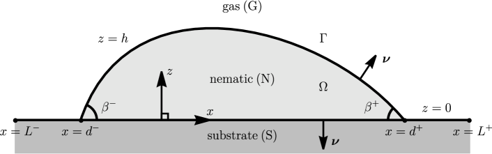
Figure 1: A schematic of a static ridge of nematic (N) resting on an ideal solid substrate (S) at $\displaystyle z=0$, $\displaystyle L^{-}\leq x\leq L^{+}$, in an atmosphere of passive gas (G), with gas–nematic interface at $\displaystyle z=h$ and contact lines at $\displaystyle x=d^{\pm}$. The Cartesian coordinates $\displaystyle x$, $\displaystyle y$ and $\displaystyle z$ (where the $\displaystyle y$-direction is into the page), the region of nematic in the $\displaystyle(x,z)$-plane $\displaystyle\Omega$ bounded by the interface $\displaystyle\Gamma$, the outward unit normals $\displaystyle\bm{\nu}$ and the contact angles $\displaystyle\beta^{\pm}$ are also indicated.

As described in the previous section, we consider a static ridge of nematic (N) resting on an ideal solid substrate (S) in an atmosphere of passive gas (G), as shown in Figure 1, which also indicates the Cartesian coordinates $\displaystyle x$, $\displaystyle y$ and $\displaystyle z$ that we use. The region of nematic in the $\displaystyle(x,z)$-plane $\displaystyle\Omega$ is bounded by the interface $\displaystyle\Gamma$, which consists of the gas–nematic interface at $\displaystyle z=h(x)$, denoted by $\displaystyle\Gamma_{\rm GN}$, and the nematic–substrate interface at $\displaystyle z=0$, denoted by $\displaystyle\Gamma_{\rm NS}$, and has two nematic–substrate–gas three-phase contact lines at $\displaystyle x=d^{-}$ and $\displaystyle x=d^{+}$. We assume that the ridge height $\displaystyle h$ and the position of the contact lines do not vary in the $\displaystyle y$-direction, so that the contact lines form two infinitely-long parallel lines in the $\displaystyle y$-direction and the ridge height $\displaystyle h$ is subject to the boundary conditions $\displaystyle h(d^{\pm})=0$. We also assume that the director $\displaystyle\bm{n}$ is confined to the $\displaystyle(x,z)$-plane, and hence takes the form

$$\displaystyle\bm{n}=\cos\theta\,\bm{\hat{x}}+\sin\theta\,\bm{\hat{z}},$$ (1)

where $\displaystyle\bm{\hat{x}}$ and $\displaystyle\bm{\hat{z}}$ are the Cartesian coordinate unit vectors in the $\displaystyle x$- and $\displaystyle z$-directions, respectively, and $\displaystyle\theta=\theta(x,z)$ is the director angle, which also does not vary in the $\displaystyle y$-direction.

The outward unit normals of the interfaces $\displaystyle\Gamma_{\rm GN}$ and $\displaystyle\Gamma_{\rm NS}$, which we denote by $\displaystyle\bm{\nu}_{\rm GN}$ and $\displaystyle\bm{\nu}_{\rm NS}$, are given by

$$\displaystyle\bm{\nu}_{\rm GN} \displaystyle=-\dfrac{{h}_{x}}{\sqrt{1+{h}_{x}^{2}}}\bm{\hat{x}}+\dfrac{1}{\sqrt{1+{h}_{x}^{2}}}\bm{\hat{z}},$$ (2)

$$\displaystyle\bm{\nu}_{\rm NS} \displaystyle=-\bm{\hat{z}},$$ (3)

respectively, where the subscript $\displaystyle x$ denotes differentiation with respect to $\displaystyle x$. These two interfaces meet the gas–substrate interface, denoted by $\displaystyle\Gamma_{\rm GS}$, at the two contact lines $\displaystyle x=d^{\pm}$. The left-hand and right-hand edges of the substrate are at $\displaystyle x=L^{-}(<d^{-})$ and $\displaystyle x=L^{+}(>d^{+})$, respectively, as shown in Figure 1. The contact angles formed between $\displaystyle\Gamma_{\rm GN}$ and $\displaystyle\Gamma_{\rm NS}$ at $\displaystyle x=d^{-}$ and $\displaystyle x=d^{+}$ are denoted by $\displaystyle\beta^{-}$ and $\displaystyle\beta^{+}$, respectively, and satisfy

$$\displaystyle\tan\beta^{\pm} \displaystyle=\mp h_{x}\quad\text{at}\quad x=d^{\pm}.$$ (4)

We note that there is, in general, no requirement for $\displaystyle h$ to be symmetric about its midpoint and, in particular, no requirement for the contact angles to be the same.

In general, we do not fix either the contact line positions or the contact angles, and allow $\displaystyle d^{\pm}$ and $\displaystyle\beta^{\pm}$ to be unknowns. However, if the substrate has been treated in such a way as either to pin the contact lines or to fix the contact angles, then either $\displaystyle d^{\pm}$ or $\displaystyle\beta^{\pm}$, respectively, are prescribed and the nematic Young equations, which will be derived shortly, are not relevant. The ridge has a prescribed constant cross-sectional area $\displaystyle A$ in the $\displaystyle(x,z)$-plane, so that

$$\displaystyle\iint\,\differential\Omega \displaystyle=A.$$ (5)

As mentioned in Section 1, we include the effects of gravity. Specifically, we assume the gravity acts in the $\displaystyle(x,z)$-plane but, in order to keep the setup as general as possible, do not specify its direction.

In Section 3 we obtain the complete theoretical description for this system using the calculus of variations assuming that the ridge height $\displaystyle h$ is a single-valued function of $\displaystyle x$. A necessary, but not sufficient, condition for this to be valid is that the contact angles are acute (i.e. that $\displaystyle 0\leq\beta^{\pm}\leq\pi/2$). We have performed the corresponding derivation when the ridge height $\displaystyle h$ is a double-valued function of $\displaystyle x$. However, since this derivation involves either splitting the gas–nematic interface into three parts in each of which $\displaystyle h$ is a single-valued function of $\displaystyle x$ or using a different coordinate system, for simplicity of presentation, and because many of the situations described in Section 1 involve small contact angles, in the present work we describe the details of the derivation only when $\displaystyle h$ is a single-valued function of $\displaystyle x$. The details of the corresponding derivation when $\displaystyle h$ is a double-valued function of $\displaystyle x$ are given by Cousins [47].

3 Constrained minimisation of the free energy

Using the calculus of variations we minimise the free energy of the system $\displaystyle E$ (per unit length in the $\displaystyle y$-direction) subject to the area constraint 5 and the boundary conditions $\displaystyle h(d^{\pm})=0$ to obtain the governing equations for a ridge of nematic in terms of the four unknowns $\displaystyle\theta(x,z)$, $\displaystyle h(x)$, $\displaystyle d^{-}$ and $\displaystyle d^{+}$, and a Lagrange multiplier associated with the area constraint 5, the latter of which we denote by $\displaystyle p_{0}$. The unknown contact angles $\displaystyle\beta^{\pm}$ are obtained from the slope of the ridge height $\displaystyle h_{x}$ using 4. The free energy of the system $\displaystyle E$ is the sum of the bulk elastic energy of the nematic, denoted by $\displaystyle E_{\rm bulk}$, and the interface energies, denoted by $\displaystyle E_{\rm GN}$, $\displaystyle E_{\rm NS}$ and $\displaystyle E_{\rm GS}$, for the interfaces $\displaystyle\Gamma_{\rm GN}$, $\displaystyle\Gamma_{\rm NS}$ and $\displaystyle\Gamma_{\rm GS}$, respectively, where

$$\displaystyle E_{\rm bulk} \displaystyle=\int^{d^{+}}_{d^{-}}\int^{h}_{0}\Big{(}W(\theta,\theta_{x},\theta_{z})+\psi_{\rm g}\Big{)}\,\,\differential z\,\differential x,$$ (6)

$$\displaystyle E_{\rm GN} \displaystyle=\int^{d^{+}}_{d^{-}}\sqrt{1+h_{x}^{2}}\,\big{[}\omega_{\rm GN}(\theta,h_{x})\big{]}^{z=h}\,\differential x,$$ (7)

$$\displaystyle E_{\rm NS} \displaystyle=\int^{d^{+}}_{d^{-}}\big{[}\omega_{\rm NS}(\theta)\big{]}^{z=0}\,\,\differential x,$$ (8)

$$\displaystyle E_{\rm GS} \displaystyle=\int^{d^{-}}_{L^{-}}\big{[}\omega_{\rm GS}\big{]}^{z=0}\,\,\differential x+\int^{L^{+}}_{d^{+}}\big{[}\omega_{\rm GS}\big{]}^{z=0}\,\,\differential x.$$ (9)

In 6 the bulk elastic energy density $\displaystyle W(\theta,\theta_{x},\theta_{z})$ is assumed to depend on the director angle $\displaystyle\theta$ and on elastic distortions of the director via the spatial derivatives of $\displaystyle\theta$ [19]. Also in 6, the gravitational potential energy density $\displaystyle\psi_{\rm g}(x,z)$ is allowed to depend on one or both of the Cartesian coordinates $\displaystyle x$ and $\displaystyle z$. In 7 and 8 the interface energy densities $\displaystyle\omega_{\rm GN}(\theta,h_{x})$ and $\displaystyle\omega_{\rm NS}(\theta)$ are assumed to be in the form of the Rapini–Papoular energy density [45], which depends on the angle between the director 1 and the outward unit normal of the interfaces, namely 2 and 3, respectively. In 9 the interface energy density $\displaystyle\omega_{\rm GS}$ takes a constant value.

We define the functional $\displaystyle F=F(\theta,\theta_{x},\theta_{z},h,h_{x},d^{-},d^{+})=E+\mathcal{C}_{\rm area}$ as the sum of the free energy of the system $\displaystyle E$ and a term $\displaystyle\mathcal{C}_{\rm area}$, corresponding to the area constraint 5, given by

$$\displaystyle\mathcal{C}_{\rm area} \displaystyle=p_{0}\times\left(A-\int^{d^{+}}_{d^{-}}\int^{h}_{0}\,\differential z\,\differential x\right),$$ (10)

so that the functional $\displaystyle F$ is given by

$$\displaystyle F=E_{\rm bulk}+E_{\rm GN}+E_{\rm NS}+E_{\rm GS}+\mathcal{C}_{\rm area}.$$ (11)

We now consider the variation of $\displaystyle F$, given by 11 with 6, 7, 8, 9 and 10, with respect to small variations of the variables $\displaystyle\theta$, $\displaystyle h$, $\displaystyle d^{-}$ and $\displaystyle d^{+}$ of the form

$$\displaystyle\theta\to\theta+\delta_{\theta},\quad h\to h+\delta_{h},\quad d^{-}\to d^{-}+\delta_{d^{-}},\quad d^{+}\to d^{+}+\delta_{d^{+}}.$$ (12)

There are no constraints on the director angle $\displaystyle\theta$, and therefore there are no constraints on its variation $\displaystyle\delta_{\theta}$. There is, however, a constraint on the ridge height $\displaystyle h$ because of the boundary conditions $\displaystyle h(d^{\pm})=0$, so that the variation of the ridge height $\displaystyle\delta_{h}$ at the contact lines satisfies

$$\displaystyle\delta_{h} \displaystyle=-{h}_{x}\delta_{d^{-}}=-\tan\beta^{-}\,\delta_{d^{-}}\quad\text{at}\quad x=d^{-},$$ (13)

$$\displaystyle\delta_{h} \displaystyle=-{h}_{x}\delta_{d^{+}}=+\tan\beta^{+}\,\delta_{d^{+}}\quad\text{at}\quad x=d^{+}.$$ (14)

The variation of the functional $\displaystyle F$, denoted by $\displaystyle\delta F$, is given by

$$\displaystyle\delta F \displaystyle=F\left(\theta+\delta_{\theta},(\theta+\delta_{\theta})_{x},(\theta+\delta_{\theta})_{z},h+\delta_{h},(h+\delta_{h})_{x},d^{-}+\delta_{d^{-}},d^{+}+\delta_{d^{+}})\right.$$

$$\displaystyle\qquad\qquad\left.-F(\theta,\theta_{x},\theta_{z},h,h_{x},d^{-},d^{+}\right).$$ (15)

We now consider the variation of each term in 11 in turn, and neglect terms in 15 that are quadratic in the variations $\displaystyle\delta_{\theta}$, $\displaystyle\delta_{h}$, $\displaystyle\delta_{d^{-}}$ and $\displaystyle\delta_{d^{+}}$.

For the bulk elastic energy $\displaystyle E_{\rm bulk}$, given by 6, $\displaystyle\delta E_{\rm bulk}$ is given by

$$\displaystyle\delta E_{\rm bulk} \displaystyle=\int^{d^{+}}_{d^{-}}\int^{h}_{0}\delta_{\theta}\partialderivative{W}{\theta}+{\delta_{\theta}}_{x}\partialderivative{W}{\theta_{x}}+{\delta_{\theta}}_{z}\partialderivative{W}{\theta_{z}}\,\,\differential z\,\differential x+\int^{d^{+}}_{d^{-}}\delta_{h}\left[W+\psi_{\rm g}\right]^{z=h}\,\,\differential x$$

$$\displaystyle\quad\quad-\delta_{d^{-}}\Bigg{[}\int^{h}_{0}(W+\psi_{\rm g})\,\,\differential z\Bigg{]}^{x=d^{-}}+\delta_{d^{+}}\Bigg{[}\int^{h}_{0}(W+\psi_{\rm g})\,\,\differential z\Bigg{]}^{x=d^{+}}.$$ (16)

Since $\displaystyle h(d^{\pm})=0$, the last two terms in 16 are identically zero. The terms in 16 containing derivatives of $\displaystyle\delta_{\theta}$, namely $\displaystyle{\delta_{\theta}}_{x}$ and $\displaystyle{\delta_{\theta}}_{z}$, are transformed into terms involving $\displaystyle\delta_{\theta}$ by using the divergence theorem, namely

$$\displaystyle\int\int{\delta_{\theta}}_{\alpha}\partialderivative{W}{\theta_{\alpha}}\,\differential\Omega \displaystyle=\oint_{\Gamma}\delta_{\theta}\partialderivative{W}{\theta_{\alpha}}\bm{\hat{\alpha}}\cdot\bm{\nu}\,\differential\Gamma-\int\int\delta_{\theta}\partialderivative{\alpha}\left(\partialderivative{W}{\theta_{\alpha}}\right)\,\differential\Omega,$$ (17)

where $\displaystyle\alpha=x$ or $\displaystyle\alpha=z$. The line integral along $\displaystyle\Gamma$ in 17 is composed of a component along $\displaystyle\Gamma_{\rm GN}$ from $\displaystyle x=d^{+}$ to $\displaystyle x=d^{-}$ on $\displaystyle z=h$ with $\displaystyle\differential\Gamma=-\sqrt{1+{h}_{x}^{2}}\,\differential x$ and outward unit normal 3, and a component along $\displaystyle\Gamma_{\rm NS}$ at $\displaystyle z=0$ from $\displaystyle x=d^{-}$ to $\displaystyle x=d^{+}$ with $\displaystyle\differential\Gamma=\differential x$ and outward unit normal 2, and is given explicitly by

$$\displaystyle\oint_{\Gamma}\delta_{\theta}\partialderivative{W}{\theta_{\alpha}}\bm{\hat{\alpha}}\cdot\bm{\nu}\,\differential\Gamma \displaystyle=\int^{d^{-}}_{d^{+}}\Bigg{[}\delta_{\theta}\partialderivative{W}{\theta_{\alpha}}\Bigg{]}^{z=h}\bm{\hat{\alpha}}\cdot(h_{x}\bm{\hat{z}}-\bm{\hat{z}})\,\,\differential x-\int^{d^{+}}_{d^{-}}\Bigg{[}\delta_{\theta}\partialderivative{W}{\theta_{\alpha}}\Bigg{]}^{z=0}\bm{\hat{\alpha}}\cdot\bm{\hat{z}}\,\,\differential x.$$ (18)

Equations 16–18 can be combined and rearranged to express the variation $\displaystyle\delta E_{\rm bulk}$ as

$$\displaystyle\delta E_{\rm bulk} \displaystyle=\int^{d^{+}}_{d^{-}}\int^{h}_{0}\delta_{\theta}\left(\partialderivative{W}{\theta}-\partialderivative{x}\left(\partialderivative{W}{\theta_{x}}\right)-\partialderivative{z}\left(\partialderivative{W}{\theta_{z}}\right)\right)\,\differential z\,\differential x$$

$$\displaystyle\quad\quad+\int^{d^{+}}_{d^{-}}\delta_{h}\left[W+\psi_{\rm g}\right]^{z=h}\,\,\differential x-\int_{d^{-}}^{d^{+}}\left[\delta_{\theta}h_{x}\partialderivative{W}{\theta_{x}}\right]^{z=h}\,\,\differential x$$ (19)

$$\displaystyle\quad\quad+\int_{d^{-}}^{d^{+}}\left[\delta_{\theta}\partialderivative{W}{\theta_{z}}\right]^{z=h}\,\,\differential x-\int_{d^{-}}^{d^{+}}\left[\delta_{\theta}\partialderivative{W}{\theta_{z}}\right]^{z=0}\differential x.$$

For the gas–nematic interface energy $\displaystyle E_{\rm GN}$, given by 7, carrying out integration by parts on the terms involving $\displaystyle{\delta_{h}}_{x}$ shows that $\displaystyle\delta E_{\rm GN}$ is given by

$$\displaystyle\delta E_{\rm GN} \displaystyle=\int^{d^{+}}_{d^{-}}\left[\delta_{\theta}\sqrt{1+{h}_{x}^{2}}\partialderivative{\omega_{\rm GN}}{\theta}+\delta_{h}\left(\sqrt{1+{h}_{x}^{2}}\partialderivative{\omega_{\rm GN}}{\theta}\partialderivative{\theta}{z}-\partialderivative{x}\Big{[}\partialderivative{{h}_{x}}\big{(}\sqrt{1+{h}_{x}^{2}}\,\,\omega_{\rm GN}\big{)}\Big{]}\right)\right]^{z=h}\,\differential x$$

$$\displaystyle\quad\quad-\delta_{d^{-}}\left[\sqrt{1+{h}_{x}^{2}}\,\omega_{\rm GN}\right]^{x=d^{-}}+\delta_{d^{+}}\left[\sqrt{1+{h}_{x}^{2}}\,\omega_{\rm GN}\right]^{x=d^{+}}$$ (20)

$$\displaystyle\quad\quad-\left[\delta_{h}\partialderivative{{h}_{x}}\left(\sqrt{1+{h}_{x}^{2}}\,\,\omega_{\rm GN}\right)\right]^{x=d^{-}}+\left[\delta_{h}\partialderivative{{h}_{x}}\left(\sqrt{1+{h}_{x}^{2}}\,\,\omega_{\rm GN}\right)\right]^{x=d^{+}}.$$

Substituting for the variation of the ridge height $\displaystyle\delta_{h}$ at the contact lines, given by 13 and 14, then yields

$$\displaystyle\delta E_{\rm GN} \displaystyle=\int^{d^{+}}_{d^{-}}\Bigg{[}\delta_{\theta}\sqrt{1+{h}_{x}^{2}}\partialderivative{\omega_{\rm GN}}{\theta}+\delta_{h}\left(\sqrt{1+{h}_{x}^{2}}\partialderivative{\omega_{\rm GN}}{\theta}\partialderivative{\theta}{z}-\partialderivative{x}\Big{[}\partialderivative{{h}_{x}}\big{(}\sqrt{1+{h}_{x}^{2}}\,\,\omega_{\rm GN}\big{)}\Big{]}\right)\Bigg{]}^{z=h}\,\differential x$$

$$\displaystyle\quad\quad-\delta_{d^{-}}\left[\sqrt{1+{h}_{x}^{2}}\,\omega_{\rm GN}-{h}_{x}\partialderivative{{h}_{x}}\left(\sqrt{1+{h}_{x}^{2}}\,\omega_{\rm GN}\right)\right]^{x=d^{-}}$$ (21)

$$\displaystyle\quad\quad+\delta_{d^{+}}\left[\sqrt{1+{h}_{x}^{2}}\,\omega_{\rm GN}-{h}_{x}\partialderivative{{h}_{x}}\left(\sqrt{1+{h}_{x}^{2}}\,\omega_{\rm GN}\right)\right]^{x=d^{+}}.$$

For the nematic–substrate interface energy $\displaystyle E_{\rm NS}$, given by 8, $\displaystyle\delta E_{\rm NS}$ is given by

$$\displaystyle\delta E_{\rm NS} \displaystyle=\int^{d^{+}}_{d^{-}}\left[\delta_{\theta}\partialderivative{\omega_{\rm NS}}{\theta}\right]^{z=0}\,\,\differential x-\delta_{d^{-}}\left[\omega_{\rm NS}\right]^{x=d^{-}}+\delta_{d^{+}}\left[\omega_{\rm NS}\right]^{x=d^{+}}.$$ (22)

For the gas–substrate interface energy $\displaystyle E_{\rm GS}$, given by 9, $\displaystyle\delta E_{\rm GS}$ is given by

$$\displaystyle\delta E_{\rm GS} \displaystyle=\delta_{d^{-}}\left[\omega_{\rm GS}\right]^{x=d^{-}}-\delta_{d^{+}}\left[\omega_{\rm GS}\right]^{x=d^{+}}.$$ (23)

Finally, for the area constraint term $\displaystyle\mathcal{C}_{\rm area}$, given by 10, using the boundary conditions $\displaystyle h(d^{\pm})=0$ shows that $\displaystyle\delta\mathcal{C}_{\rm area}$ is given by

$$\displaystyle\delta\mathcal{C}_{\rm area} \displaystyle=-\int^{d^{+}}_{d^{-}}\delta_{h}\,p_{0}\,\,\differential x.$$ (24)

The variation of $\displaystyle F$ is obtained by adding the terms from each of the individual variations, given by 19 and 21–24, so that

$$\displaystyle\delta F=\delta E_{\rm bulk}+\delta E_{\rm GN}+\delta E_{\rm NS}+\delta E_{\rm GS}+\delta\mathcal{C}_{\rm area}.$$ (25)

Since we seek extrema of the free energy $\displaystyle E$ for which $\displaystyle\delta F=0$, and the variations $\displaystyle\delta_{\theta}$, $\displaystyle\left[\delta_{\theta}\right]^{z=0}$, $\displaystyle\left[\delta_{\theta}\right]^{z=h}$, $\displaystyle\delta_{h}$, $\displaystyle\delta_{d^{-}}$ and $\displaystyle\delta_{d^{+}}$ are independent and arbitrary, their coefficients in $\displaystyle\delta F$, given by 25, must be zero. Together with the area constraint 5 and the boundary conditions $\displaystyle h(d^{\pm})=0$, the coefficients of each variation yield the governing equations for a nematic ridge, as described in the next section.

4 Governing equations for a nematic ridge

Each of the six governing equations derived from setting the coefficients of $\displaystyle\delta_{\theta}$, $\displaystyle\left[\delta_{\theta}\right]^{z=0}$, $\displaystyle\left[\delta_{\theta}\right]^{z=h}$, $\displaystyle\delta_{h}$, $\displaystyle\delta_{d^{-}}$ and $\displaystyle\delta_{d^{+}}$ in 25 to zero has a distinct physical interpretation, namely the balance of elastic torque within the bulk of the nematic, the balance-of-couple conditions on the gas–nematic and nematic–substrate interfaces, the balance-of-stress condition on the gas–nematic interface, and the balance-of-stress conditions at the contact lines, respectively. These equations are summarised below.

The balance of elastic torque within the bulk of the nematic, i.e. the Euler–Lagrange equation, for the elastic free energy density $\displaystyle W$, is

$$\displaystyle\partialderivative{W}{\theta}-\partialderivative{x}\left(\partialderivative{W}{\theta_{x}}\right)-\partialderivative{z}\left(\partialderivative{W}{\theta_{z}}\right) \displaystyle=0.$$ (26)

The balance-of-couple conditions on the gas–nematic interface and the nematic–substrate interface, namely the weak anchoring conditions [19, 48], are given by

$$\displaystyle\partialderivative{W}{\theta_{z}}-{h}_{x}\,\partialderivative{W}{\theta_{x}}+\sqrt{1+{h}_{x}^{2}}\,\partialderivative{\omega_{\rm GN}}{\theta} \displaystyle=0\quad\text{on}\quad z=h$$ (27)

and

$$\displaystyle-\partialderivative{W}{\theta_{z}}+\partialderivative{\omega_{\rm NS}}{\theta} \displaystyle=0\quad\text{on}\quad z=0,$$ (28)

respectively.

The balance-of-stress condition on the gas–nematic interface is given by

$$\displaystyle W+\psi_{\rm g}-p_{0}+\sqrt{1+{h}_{x}^{2}}\,\partialderivative{\omega_{\rm GN}}{\theta}\partialderivative{\theta}{z}-\partialderivative{x}\left(\partialderivative{{h}_{x}}\left(\sqrt{1+{h}_{x}^{2}}\,\,\omega_{\rm GN}\right)\right) \displaystyle=0\quad\text{on}\quad z=h.$$ (29)

To distinguish equation 29 from the classical isotropic Young–Laplace equation [15], henceforth it is referred to as the nematic Young–Laplace equation.

The balance-of-stress conditions at the contact lines are given by

$$\displaystyle\omega_{\rm NS}-\omega_{\rm GS}+\sqrt{1+{h}_{x}^{2}}\,\omega_{\rm GN}-{h}_{x}\partialderivative{{h}_{x}}\left(\sqrt{1+{h}_{x}^{2}}\,\omega_{\rm GN}\right) \displaystyle=0\quad\text{at}\quad x=d^{\pm}.$$ (30)

To distinguish equations 30 from the classical isotropic Young equations [15], henceforth they are referred to as the nematic Young equations.

Once explicit forms of the energy densities $\displaystyle W$, $\displaystyle\psi_{\rm g}$, $\displaystyle\omega_{\rm GN}$, $\displaystyle\omega_{\rm NS}$ and $\displaystyle\omega_{\rm GS}$ have been prescribed, the balance of elastic torque within the bulk of the nematic 26, the three interface conditions 28, 27 and 29, the two nematic Young equations 30, the area constraint 5, and the two boundary conditions $\displaystyle h(d^{\pm})=0$ provide the complete theoretical description for a static ridge of nematic in terms of the five unknowns $\displaystyle\theta(x,z)$, $\displaystyle h(x)$, $\displaystyle d^{-}$, $\displaystyle d^{+}$ and $\displaystyle p_{0}$.

4.1 The bulk elastic energy density and the interface energy densities

As mentioned in Section 1, for the bulk elastic energy density $\displaystyle W$ we use the standard Oseen–Frank bulk elastic energy density [19] for which

$$\displaystyle W \displaystyle=\dfrac{1}{2}K_{1}(\nabla\cdot\bm{n})^{2}+\dfrac{1}{2}K_{2}(\bm{n}\cdot\nabla\times\bm{n})^{2}+\dfrac{1}{2}K_{3}(\bm{n}\times\nabla\times\bm{n})^{2}$$

$$\displaystyle\quad\quad+\dfrac{1}{2}(K_{2}+K_{4})\nabla\cdot\big{[}(\bm{n}\cdot\nabla)\bm{n}-(\nabla\cdot\bm{n})\bm{n}\big{]},$$ (31)

where $\displaystyle K_{1}$, $\displaystyle K_{2}$, $\displaystyle K_{3}$, and the combination $\displaystyle K_{2}+K_{4}$ are called the splay, twist, bend, and saddle-splay elastic constants, respectively, and $\displaystyle\nabla=(\partial/\partial x,\partial/\partial y,\partial/\partial z)$. Substituting 1 into 31 yields

$$\displaystyle W(\theta,\theta_{x},\theta_{z}) \displaystyle=\dfrac{K_{1}}{2}\left(\theta_{z}\cos\theta-\theta_{x}\sin\theta\right)^{2}+\dfrac{K_{3}}{2}\left(\theta_{x}\cos\theta+\theta_{z}\sin\theta\right)^{2},$$ (32)

which depends only on the splay and bend elastic deformations. Although we use the full Oseen–Frank energy density 32, we note that the commonly used one-constant approximation of the elastic constants [19] can be implemented in 32 by setting $\displaystyle K=K_{1}=K_{3}$, in which case $\displaystyle W(\theta_{x},\theta_{z})=K(\theta_{x}^{2}+\theta_{z}^{2})/2$.

As also mentioned in Section 1, for $\displaystyle\omega_{\rm GN}$ and $\displaystyle\omega_{\rm NS}$ we use the standard Rapini–Papoular form [45] for which

$$\displaystyle\omega_{\rm GN} \displaystyle=\gamma_{\rm GN}+\dfrac{C_{\rm GN}}{4}\left(1-2(\bm{\nu}_{\rm GN}\cdot\bm{n})^{2}\right),$$ (33)

$$\displaystyle\omega_{\rm NS} \displaystyle=\gamma_{\rm NS}+\dfrac{C_{\rm NS}}{4}\left(1-2(\bm{\nu}_{\rm NS}\cdot\bm{n})^{2}\right),$$ (34)

where $\displaystyle C_{\rm GN}$ and $\displaystyle\gamma_{\rm GN}$ are the anchoring strength and isotropic interfacial tension for the gas–nematic (GN) interface, respectively, and $\displaystyle C_{\rm NS}$ and $\displaystyle\gamma_{\rm NS}$ are the anchoring strength and isotropic interfacial tension for the nematic–substrate (NS) interface, respectively. The Rapini–Papoular form ensures that the interface energy densities $\displaystyle\omega_{\rm GN}$ and $\displaystyle\omega_{\rm NS}$ are at a minimum when $\displaystyle\bm{n}$ and $\displaystyle\bm{\nu}$ are parallel for $\displaystyle C_{\rm GN}>0$ and $\displaystyle C_{\rm NS}>0$, respectively, and at a minimum when $\displaystyle\bm{n}$ and $\displaystyle\bm{\nu}$ are perpendicular for $\displaystyle C_{\rm GN}<0$ and $\displaystyle C_{\rm NS}<0$, respectively. Therefore weak homeotropic anchoring occurs on the gas–nematic interface when $\displaystyle C_{\rm GN}>0$ and on the nematic–substrate interface when $\displaystyle C_{\rm NS}>0$, and weak planar anchoring occurs on the gas–nematic interface when $\displaystyle C_{\rm GN}<0$ and on the nematic–substrate interface when $\displaystyle C_{\rm NS}<0$. Substituting 2 and 3 into 33 and 34 yields

$$\displaystyle\omega_{\rm GN}(\theta,{h}_{x}) \displaystyle=\gamma_{\rm GN}+\dfrac{C_{\rm GN}}{4}\left[\dfrac{1-{h}_{x}^{2}}{1+{h}_{x}^{2}}\cos 2\theta+\dfrac{2{h}_{x}}{1+{h}_{x}^{2}}\sin 2\theta\right],$$ (35)

$$\displaystyle\omega_{\rm NS}(\theta) \displaystyle=\gamma_{\rm NS}+\dfrac{C_{\rm NS}}{4}\cos 2\theta.$$ (36)

Experimental techniques for the measurement of $\displaystyle C_{\rm NS}$ are well established [49, 50, 51], and values in the range $\displaystyle|C_{\rm NS}|=10^{-6}$–$\displaystyle 10^{-3}\,$N m^-1 have been reported for a variety of nematic materials and substrates with planar or homeotropic anchoring [49, 50, 7]. Measurements of $\displaystyle C_{\rm GN}$ are less common [7]; however, the reported values of $\displaystyle C_{\rm GN}>10^{-5}\,{\rm Nm}^{-1}$ between air and the nematic mixture ZLI 2860 [52] and of $\displaystyle C_{\rm GN}>10^{-4}\,{\rm Nm}^{-1}$ between air and the nematic p-methoxy-benzylidene-p-n-butyl aniline (MBBA) [53] suggest that $\displaystyle C_{\rm GN}$ and $\displaystyle C_{\rm NS}$ can be of comparable magnitude. In standard low-molecular-mass nematics, the isotropic interfacial tensions (i.e. $\displaystyle\gamma_{\rm GN}$ and $\displaystyle\gamma_{\rm NS}$) are typically much larger than the magnitudes of the anchoring strengths (i.e. $\displaystyle|C_{\rm GN}|$ and $\displaystyle|C_{\rm NS}|$) [7]. For example, the isotropic interfacial tension of an interface between air and the nematic 4-Cyano-4’-pentylbiphenyl (5CB) has been measured as $\displaystyle\gamma_{\rm GN}=4.0\times 10^{-2}\,{\rm N\,m}^{-1}$, and the isotropic interfacial tension of an interface between the substrate poly(methyl methacrylate) (PMMA) and 5CB has been measured as $\displaystyle\gamma_{\rm NS}=4.051\times 10^{-2}\,{\rm N\,m}^{-1}$ [54].

The gas–substrate interface has constant energy density

$$\displaystyle\omega_{\rm GS}=\gamma_{\rm GS},$$ (37)

where $\displaystyle\gamma_{\rm GS}$ is the isotropic interfacial tension of the gas–substrate interface.

4.2 Governing equations using the Oseen–Frank bulk elastic energy density and the Rapini–Papoular interface energy densities

Using 32 in 26 yields the balance of elastic torque within the bulk of the nematic,

$$\displaystyle(K_{1}\sin^{2}\theta+K_{3}\cos^{2}\theta)\theta_{xx}+(K_{1}\cos^{2}\theta+K_{3}\sin^{2}\theta)\theta_{zz}$$ (38)

$$\displaystyle\quad\quad+(K_{3}-K_{1})\Big{[}\left(\theta_{z}\cos\theta-\theta_{x}\sin\theta\right)\left(\theta_{x}\cos\theta+\theta_{z}\sin\theta\right)+\theta_{xz}\sin 2\theta\Big{]}=0.$$

Using 32 and 35 in 27 yields the balance-of-couple condition on the gas–nematic interface,

$$\displaystyle\left(K_{1}\cos^{2}\theta+K_{3}\sin^{2}\theta\right)\theta_{z}+\dfrac{1}{2}(K_{3}-K_{1})(\theta_{x}-h_{x}\theta_{z})\sin 2\theta-\left(K_{1}\sin^{2}\theta+K_{3}\cos^{2}\theta\right)h_{x}\theta_{x}$$

$$\displaystyle\quad\quad+\dfrac{C_{\rm GN}}{2\sqrt{1+{h}_{x}^{2}}}\left[({h}_{x}^{2}-1)\sin 2\theta+2{h}_{x}\cos 2\theta\right]=0\quad\text{on}\quad z=h,$$ (39)

while using 36 in 28 yields the balance-of-couple condition on the nematic–substrate interface,

$$\displaystyle-\left(K_{1}\cos^{2}\theta+K_{3}\sin^{2}\theta\right)\theta_{z}-\dfrac{1}{2}(K_{3}-K_{1})\theta_{x}\sin 2\theta-\dfrac{C_{\rm NS}}{2}\sin 2\theta=0\quad\text{on}\quad z=0.$$ (40)

Using 32 and 35 in 29 yields the nematic Young–Laplace equation,

$$\displaystyle p_{0}-W-\psi_{\rm g}+\gamma_{\rm GN}\dfrac{{h}_{xx}}{\left(1+{h}_{x}^{2}\right)^{3/2}}+\dfrac{C_{\rm GN}}{4\left(1+{h}_{x}^{2}\right)^{5/2}}\Bigg{[}3{h}_{xx}\Big{[}({h}_{x}^{2}-1)\cos 2\theta-2{h}_{x}\sin 2\theta\Big{]}$$

$$\displaystyle\quad\quad+(1+{h}_{x}^{2})\bigg{(}4\cos 2\theta\Big{[}\theta_{x}-h_{x}(1+{h}_{x}^{2})\theta_{z}\Big{]}+2\sin 2\theta\Big{[}(1-{h}_{x}^{4})\theta_{z}+{h}_{x}(3+{h}_{x}^{2})\theta_{x}\Big{]}\bigg{)}\Bigg{]}=0$$

$$\displaystyle\hskip 271.72389pt\text{on}\quad z={h}.$$ (41)

In order to express the nematic Young equations 30 in terms of the contact angles $\displaystyle\beta^{\pm}$, we use the relations 4. Then, using 35, 36 and 37 in 30 yields

$$\displaystyle\gamma_{\rm GS}-\gamma_{\rm NS}-\gamma_{\rm GN}\cos\beta^{-} \displaystyle=\dfrac{C_{\rm NS}}{4}\cos 2\theta+\dfrac{C_{\rm GN}}{4}\left[\cos 2(\theta-\beta^{-})\cos\beta^{-}-2\sin 2(\theta-\beta^{-})\sin\beta^{-}\right]$$

$$\displaystyle\qquad\qquad\qquad\qquad\qquad\qquad\qquad\qquad\qquad\qquad\text{at}\quad x=d^{-},$$ (42)

$$\displaystyle\gamma_{\rm GS}-\gamma_{\rm NS}-\gamma_{\rm GN}\cos\beta^{+} \displaystyle=\dfrac{C_{\rm NS}}{4}\cos 2\theta+\dfrac{C_{\rm GN}}{4}\left[\cos 2(\theta+\beta^{+})\cos\beta^{+}-2\sin 2(\theta+\beta^{+})\sin\beta^{+}\right]$$

$$\displaystyle\qquad\qquad\qquad\qquad\qquad\qquad\qquad\qquad\qquad\qquad\text{at}\quad x=d^{+}.$$ (43)

The terms on the left-hand sides of 42 and 43 appear in the classical isotropic Young equations, while the terms on the right-hand sides are due to the anisotropic nature of the nematic and arise from the weak anchoring on the gas–nematic interface and on the nematic–substrate interface, respectively. In particular, the classical isotropic Young equations are recovered from the nematic Young equations 42 and 43 by setting $\displaystyle C_{\rm NS}=C_{\rm GN}=0$.

We note that, as previously mentioned, while the nematic Young equations 42 and 43 were derived assuming the ridge height $\displaystyle h$ is a single-valued function of $\displaystyle x$, they also hold when the ridge height $\displaystyle h$ is a double-valued function of $\displaystyle x$ [47].

4.3 The equilibrium states of complete wetting and complete dewetting

The governing equations derived thus far in the present manuscript describe the partial wetting state, $\displaystyle\mathbb{P}$. As mentioned in Section 1, these equations can also be used to describe the equilibrium states of complete wetting, $\displaystyle\mathbb{W}$, and of complete dewetting, $\displaystyle\mathbb{D}$. In the $\displaystyle\mathbb{W}$ state, in which the nematic forms a film that completely coats the substrate, the nematic Young equations 42 and 43 and the boundary conditions $\displaystyle h(d^{\pm})=0$ are not relevant. The behaviour of the director and gas–nematic interface for nematic films has been studied previously (see, for example, Sonin [7] and Manyuhina [14]). Similarly, for the $\displaystyle\mathbb{D}$ state, in which the gas–nematic interface forms a cylinder, the nematic Young equations 42 and 43, the boundary conditions $\displaystyle h(d^{\pm})=0$, and the balance-of-couple condition on the nematic–solid interface 40 are not relevant. In the special case in which the gas–nematic interface is a circular cylinder, the possible director configurations are the same as those in the case of a nematic confined within a circular capillary and have been extensively studied (see, for example, Kleman [55]). The limiting cases $\displaystyle\beta^{\pm}=0$ and $\displaystyle\beta^{\pm}=\pi$ correspond to the $\displaystyle\mathbb{W}$ and the $\displaystyle\mathbb{D}$ states, respectively.

As we will show in what follows, using just the nematic Young equations 42 and 43 under the assumption that anchoring breaking occurs in regions adjacent to the contact lines, we can determine the continuous and discontinuous transitions that occur between the equilibrium states of complete wetting, partial wetting, and complete dewetting. We first briefly review the behaviour of an isotropic ridge in Section 5, before analysing the corresponding behaviour of a nematic ridge in Sections 6 and 7.

5 The equilibrium states and transitions of an isotropic ridge

For a static ridge of isotropic liquid resting on an ideal solid substrate in an atmosphere of passive gas, a much simpler version of the derivation presented in Sections 2, 3 and 4, or a simple horizontal force balance at the contact lines, shows that the well-known classical isotropic Young equations [15] are given, in the present notation, by

$$\displaystyle\gamma_{\rm GS}-\gamma_{\rm IS}-\gamma_{\rm GI}\cos\beta^{\pm}=0\quad\text{at}\quad x=d^{\pm},$$ (44)

where $\displaystyle\gamma_{\rm GI}$ and $\displaystyle\gamma_{\rm IS}$ denote the isotropic interfacial tensions of the gas–isotropic liquid and isotropic liquid–substrate interfaces, respectively. In particular, 44 shows that in this case the left-hand and right-hand contact angles are always the same, i.e. $\displaystyle\beta^{-}=\beta^{+}=\beta$, say. The classical isotropic Young equations 44 can be written in terms of a single non-dimensional parameter, namely the classical isotropic spreading parameter $\displaystyle S_{\rm I}$, which is defined by

$$\displaystyle S_{\rm I}=\dfrac{\gamma_{\rm GS}-\gamma_{\rm IS}}{\gamma_{\rm GI}}-1,$$ (45)

as

$$\displaystyle S_{\rm I}+1-\cos\beta=0.$$ (46)

Specifically, 46 shows that the $\displaystyle\mathbb{P}$ state exists only when $\displaystyle-2\leq S_{\rm I}\leq 0$ and that the contact angle is then given by $\displaystyle\beta=\cos^{-1}\left(S_{\rm I}+1\right)$.

As mentioned in Sections 1 and 4.3, the equilibrium state can also be the $\displaystyle\mathbb{W}$ state, which corresponds to $\displaystyle\beta=0$, or the $\displaystyle\mathbb{D}$ state, which corresponds to $\displaystyle\beta=\pi$, for both of which equation 46 is not relevant. The classification of the $\displaystyle\mathbb{W}$, $\displaystyle\mathbb{P}$ and $\displaystyle\mathbb{D}$ states can be obtained by solving the classical isotropic Young–Laplace equation and expressing the minimum energy state in terms of $\displaystyle S_{\rm I}$ [46, 15]. In particular, the minimum energy state is the $\displaystyle\mathbb{W}$ state for $\displaystyle S_{\rm I}>0$, the $\displaystyle\mathbb{P}$ state for $\displaystyle-2\leq S_{\rm I}\leq 0$, and the $\displaystyle\mathbb{D}$ state for $\displaystyle S_{\rm I}<-2$. The contact angle $\displaystyle\beta$ of the minimum energy state of an isotropic ridge is plotted as a function of $\displaystyle S_{\rm I}$ in Figure 2.

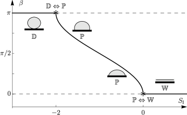
Figure 2: Summary of the solution for the contact angle $\displaystyle\beta$ as a function of the isotropic spreading parameter $\displaystyle S_{\rm I}$. The transition points are denoted by stars $\displaystyle(\mathop{\scalebox{1.5}{\raisebox{-0.86108pt}{$\displaystyle\ast$}}})$. The solid line denote the local minimum energy state and the dashed lines denote the local maximum energy states. Sketches of the minimum energy state are also shown.

We define the values of $\displaystyle S_{\rm I}$ at which there is a change in the number of possible equilibrium states as transition points. At these points, a transition occurs as $\displaystyle S_{\rm I}$ increases or decreases if the previous minimum energy state ceases to exist or a new minimum energy state comes into existence. In particular, as Figure 2 shows, for an isotropic ridge there is a change in the number of equilibrium states at the transition points $\displaystyle S_{\rm I}=-2$ and $\displaystyle S_{\rm I}=0$ which leads to continuous transitions to a new minimum energy state as $\displaystyle S_{\rm I}$ increases or decreases. For consistency with the notation used in Section 7, we denote a continuous transition between two equilibrium states for both increasing and decreasing $\displaystyle S_{\rm I}$ with a double arrow $\displaystyle(\Leftrightarrow)$. At $\displaystyle S_{\rm I}=-2$ there is a continuous transition from complete dewetting to partial wetting or vice versa, which is denoted by $\displaystyle\mathbb{D}\Leftrightarrow\mathbb{P}$. Similarly, at $\displaystyle S_{\rm I}=0$ there is a continuous transition from complete wetting to partial wetting or vice versa, which is denoted by $\displaystyle\mathbb{P}\Leftrightarrow\mathbb{W}$.

We also note that the behaviour of the contact angle for an isotropic ridge is non-hysteretic. The well-known phenomenon of isotropic contact-angle hysteresis occurs only in isotropic systems with non-ideal substrates [15], and therefore does not occur for the isotropic ridge on an ideal substrate discussed in this section.

6 The nematic Young equations

As for the isotropic ridge discussed in the previous section, for the nematic ridge considered in the present work we can use the nematic Young equations 42 and 43 to determine the continuous and discontinuous transitions that occur between the equilibrium states of complete wetting, partial wetting, and complete dewetting. At first sight, determining these transitions would appear to involve solving the governing equations for $\displaystyle\theta$ in the bulk of the nematic ridge, which would, in turn, involve solving for the ridge height $\displaystyle h$, the contact line positions $\displaystyle x=d^{\pm}$, and the Lagrange multiplier $\displaystyle p_{0}$. However, under the assumption that anchoring breaking occurs in regions adjacent to the contact lines, we can determine these continuous and discontinuous transitions from just the nematic Young equations 42 and 43.

6.1 The director orientation at the contact lines

At the contact lines the preferred director orientations on the gas–nematic and the nematic–substrate interfaces are, in general, different. Even when the anchoring is non-antagonistic (i.e. when either planar or homeotropic anchoring is preferred on both interfaces), since the preferred director orientation of both interfaces is measured relative to that interface, and the two interfaces meet at the non-zero contact angles $\displaystyle\beta^{\pm}$, the orientations are, in general, not the same. Hence the director cannot, in general, align with the preferred orientations of both interfaces. In such a situation there are three possibilities for the director orientation at the contact lines: (i) the contact angles are such that the preferred orientations on the two interfaces coincide exactly; (ii) there may be defects (disclination lines in this two-dimensional case) at one or both of the contact lines; (iii) the weak anchoring on both interfaces allows anchoring breaking to occur in regions adjacent to the contact lines and the director(s) on one or both of the interfaces deviates from the preferred alignment(s) and attains the same orientation on both interfaces.

Case (i) is a very special situation in which the contact angles are such that the preferred director orientations on the two interfaces coincide exactly at the contact lines. For instance, when the preferred orientations on the two interfaces are antagonistic, the contact angles must be exactly $\displaystyle\beta^{\pm}=\pi/2$ to allow the director to be tangent to one interface and perpendicular to the other. Since this type of special case is highly unlikely to occur in practice, we do not consider it any further in the present work.

As discussed in Section 1, case (ii) has been considered in [36] in which infinite planar anchoring was assumed on the gas–nematic and nematic–substrate interfaces. In this case, since the infinitely-strong anchoring cannot be broken, the director must adopt a splayed configuration (for a full account of splayed director configurations, see [19]) in a region adjacent to the contact line, with a disclination line located at the contact line [36]. For the finite anchoring strengths considered in the present work, we assume that the energy associated with anchoring breaking is less than the energy associated with the formation of a disclination line, and therefore that such disclination lines do not occur.

Having ruled out cases (i) and (ii), we are left with case (iii). In this case the weak anchoring on the interfaces allows anchoring breaking to occur in regions adjacent to the contact lines so that the director(s) on one or both of the interfaces deviates from the preferred alignment(s) and attains the same orientation on both interfaces.

As discussed in Section 1, for nematic films with antagonistic anchoring, when the film thickness is less than the Jenkins–Barratt–Barbero–Barberi critical thickness the energetically favourable state has a uniform director field in which the director aligns parallel to the preferred director alignment of the interface with the stronger anchoring. For a nematic ridge, close to the contact lines, where the ridge height approaches zero and hence the separation between the gas–nematic and nematic–substrate interfaces is always less than the critical thickness, anchoring breaking occurs and the director aligns parallel to the preferred alignment of the interface with the stronger anchoring. Specifically, if the nematic–substrate interface has the stronger anchoring (i.e. if $\displaystyle|C_{\rm NS}|>|C_{\rm GN}|$) then the director at the contact lines aligns parallel to the nematic–substrate interface with $\displaystyle\theta=0$ at $\displaystyle x=d^{\pm}$ in the case of planar anchoring corresponding to $\displaystyle C_{\rm NS}<0$ or perpendicular to the nematic–substrate interface with $\displaystyle\theta=\pi/2$ at $\displaystyle x=d^{\pm}$ in the case of homeotropic anchoring corresponding to $\displaystyle C_{\rm NS}>0$; we term both of these scenarios “nematic–substrate (NS) dominant anchoring”. Correspondingly, if the gas–nematic interface has the stronger anchoring (i.e. if $\displaystyle|C_{\rm GN}|>|C_{\rm NS}|$) then the director at the contact lines aligns parallel to the gas–nematic interface with $\displaystyle\theta=\beta^{\pm}$ at $\displaystyle x=d^{\pm}$ in the case of planar anchoring corresponding to $\displaystyle C_{\rm GN}<0$ or perpendicular to the gas–nematic interface with $\displaystyle\theta=\beta^{\pm}+\pi/2$ at $\displaystyle x=d^{\pm}$ in the case of homeotropic anchoring corresponding to $\displaystyle C_{\rm GN}>0$; we term both of these situations “gas–nematic (GN) dominant anchoring”.

There are two special situations in which anchoring breaking cannot occur as described above because the interfaces have either equal anchoring strengths ($\displaystyle C_{\rm NS}=C_{\rm GN}$) or equal and opposite anchoring strengths ($\displaystyle C_{\rm NS}=-C_{\rm GN}$). In both of these situations, anchoring breaking occurs on both interfaces and the director orientation adopts the average of the preferred orientations [47, 36]. In particular, when the anchoring strengths of the interfaces are equal and planar anchoring is preferred, the director angles are $\displaystyle\theta=\beta^{\pm}/2$ at $\displaystyle x=d^{\pm}$, as discussed by Rey [36], and when the anchoring strengths of the interfaces are equal and homeotropic anchoring is preferred, the director angles are $\displaystyle\theta=\beta^{\pm}/2+\pi/2$ at $\displaystyle x=d^{\pm}$. When the anchoring strengths of the interfaces are equal and opposite, the director angles are $\displaystyle\theta=\beta^{\pm}/2+\pi/4$ or $\displaystyle\theta=\beta^{\pm}/2-\pi/4$ at $\displaystyle x=d^{\pm}$.

Since for an ideal substrate the material properties of the substrate are the same at both contact lines, anchoring breaking must occur in the same way, and hence the director angles at the two contact lines must be the same. However, as we will show below, in some situations the nematic Young equations 42 and 43 allow for more than one possible contact angle for the same parameter values, and so the contact angles $\displaystyle\beta^{\pm}$ do not, in general, have to be the same and so the ridge can be asymmetric. Moreover, the contact angles $\displaystyle\beta^{\pm}$ could be different if the substrate is non-ideal and the material properties of the substrate are different at the two contact lines (for example, if the substrate was manufactured so that the values of $\displaystyle C_{\rm NS}$ at $\displaystyle x=d^{\pm}$ were different, or if gradients in the temperature of the gas or adsorption of a surfactant from the gas lead to different values of $\displaystyle C_{\rm GN}$ at $\displaystyle x=d^{\pm}$ [56]). Without loss of generality, for the remainder of the present work, we consider only the left-hand contact line, which is described by the nematic Young equation 42, and write $\displaystyle\beta^{-}=\beta$ for simplicity. The corresponding results for the right-hand contact line can be obtained in the same way.

6.2 Nematic spreading parameters

For NS-dominant anchoring (for which either $\displaystyle\theta=0$ or $\displaystyle\theta=\pi/2$) the nematic Young equation 42 reduces to a cubic equation for $\displaystyle\cos\beta$, namely either

$$\displaystyle\gamma_{\rm GS}-\left(\gamma_{\rm NS}+\tfrac{1}{4}C_{\rm NS}\right)-\left(\gamma_{\rm GN}+\tfrac{1}{4}C_{\rm GN}\right)\cos\beta=-\tfrac{1}{2}C_{\rm GN}\cos\beta\left(\cos^{2}\beta-1\right)$$ (47)

when $\displaystyle\theta=0$ or

$$\displaystyle\gamma_{\rm GS}-\left(\gamma_{\rm NS}-\tfrac{1}{4}C_{\rm NS}\right)-\left(\gamma_{\rm GN}-\tfrac{1}{4}C_{\rm GN}\right)\cos\beta=\tfrac{1}{2}C_{\rm GN}\cos\beta\left(\cos^{2}\beta-1\right)$$ (48)

when $\displaystyle\theta=\pi/2$. On the other hand, for GN-dominant anchoring (for which either $\displaystyle\theta=\beta$ or $\displaystyle\theta=\beta+\pi/2$) the nematic Young equation 42 reduces to a quadratic equation for $\displaystyle\cos\beta$, namely either

$$\displaystyle\gamma_{\rm GS}-\left(\gamma_{\rm NS}+\tfrac{1}{4}C_{\rm NS}\right)-\left(\gamma_{\rm GN}+\tfrac{1}{4}C_{\rm GN}\right)\cos\beta=\tfrac{1}{2}C_{\rm NS}\left(\cos^{2}\beta-1\right)$$ (49)

when $\displaystyle\theta=\beta$ or

$$\displaystyle\gamma_{\rm GS}-\left(\gamma_{\rm NS}-\tfrac{1}{4}C_{\rm NS}\right)-\left(\gamma_{\rm GN}-\tfrac{1}{4}C_{\rm GN}\right)\cos\beta=-\tfrac{1}{2}C_{\rm NS}\left(\cos^{2}\beta-1\right)$$ (50)

when $\displaystyle\theta=\beta+\pi/2$. Each of the equations 47, 48, 49 and 50 may each be written in terms of just two parameters as follows: 47 and 48 may be written as

$$\displaystyle S_{\rm N}+1-\cos\beta \displaystyle=-\Delta_{\rm GN}\cos\beta\left(\cos^{2}\beta-1\right),$$ (51)

while 49 and 50 may be written as

$$\displaystyle S_{\rm N}+1-\cos\beta \displaystyle=\Delta_{\rm NS}\left(\cos^{2}\beta-1\right),$$ (52)

where $\displaystyle S_{\rm N}$, $\displaystyle\Delta_{\rm NS}$ and $\displaystyle\Delta_{\rm GN}$ are defined by

$$\displaystyle S_{\rm N} \displaystyle=\dfrac{4\gamma_{\rm GS}-\left(4\gamma_{\rm NS}-|C_{\rm NS}|\right)}{4\gamma_{\rm GN}-|C_{\rm GN}|}-1,$$ (53)

$$\displaystyle\Delta_{\rm NS} \displaystyle=\dfrac{2C_{\rm NS}}{4\gamma_{\rm GN}-|C_{\rm GN}|},$$ (54)

$$\displaystyle\Delta_{\rm GN} \displaystyle=\dfrac{2C_{\rm GN}}{4\gamma_{\rm GN}-|C_{\rm GN}|},$$ (55)

respectively. Note that while the nematic spreading parameter $\displaystyle S_{\rm N}$ is the appropriate generalisation of the isotropic spreading parameter $\displaystyle S_{\rm I}$ defined in 45, the scaled anchoring coefficients $\displaystyle\Delta_{\rm NS}$ and $\displaystyle\Delta_{\rm GN}$ have no isotropic counterparts. We also note that when $\displaystyle\Delta_{\rm NS}=\Delta_{\rm GN}=0$ (i.e. when $\displaystyle C_{\rm GN}=C_{\rm NS}=0$) then $\displaystyle S_{\rm N}=(\gamma_{\rm GS}-\gamma_{\rm NS})/\gamma_{\rm GN}-1=S_{\rm I}$, and both of the nematic Young equations 51 and 52 reduce to the classical isotropic Young equation 46.

Each of the right-hand sides of the nematic Young equations 51 and 52 involve only one parameter, namely the scaled anchoring coefficients $\displaystyle\Delta_{\rm NS}$ and $\displaystyle\Delta_{\rm GN}$, respectively. At first sight, it may seem counter-intuitive that $\displaystyle\Delta_{\rm NS}$ appears in the case of GN-dominant anchoring and $\displaystyle\Delta_{\rm GN}$ appears in the case of NS-dominant anchoring. However, for GN–dominant anchoring the director is aligned with the preferred director orientation of the gas–nematic interface, and so the corresponding anchoring energy, and therefore the couple on the director, is zero. The non-zero contribution to the anchoring energy therefore derives from the breaking of the nematic–substrate interface anchoring. The corresponding explanation applies to the NS-dominant case. The right-hand sides of equations 51 and 52 may therefore be interpreted physically as the contribution to the balance of stress at the contact line associated with the breaking of the anchoring on the interface with the weaker anchoring.

7 The equilibrium states and transitions of a nematic ridge

With the director angle determined in regions adjacent to the contact lines, we can now use the nematic Young equations 51 and 52 to determine the continuous and discontinuous transitions between the $\displaystyle\mathbb{W}$, $\displaystyle\mathbb{P}$ and $\displaystyle\mathbb{D}$ states. As 51 and 52 are cubic and quadratic equations for $\displaystyle\cos\beta$, respectively, they can have up to three real solutions for $\displaystyle\beta$ and up to two real solutions for $\displaystyle\beta$, respectively. Each of these solutions for $\displaystyle\beta$ corresponds to a different $\displaystyle\mathbb{P}$ state, and therefore, unlike for the isotropic ridge described in Section 5, a nematic ridge can have multiple $\displaystyle\mathbb{P}$ states.

Following the same approach as for the isotropic ridge in Section 5, the values of $\displaystyle S_{\rm N}$ and $\displaystyle\Delta_{\rm NS}$ (for GN-dominant anchoring) or $\displaystyle S_{\rm N}$ and $\displaystyle\Delta_{\rm GN}$ (for NS-dominant anchoring) at which there is a change in the number of possible equilibrium states are again called the transition points. Specifically, a transition occurs as $\displaystyle S_{\rm N}$, $\displaystyle\Delta_{\rm NS}$ or $\displaystyle\Delta_{\rm GN}$ increases or decreases if the previous minimum energy state ceases to exist or a new minimum energy state comes into existence. In an analogous manner to that in the isotropic case, at $\displaystyle S_{\rm N}=-2$ and $\displaystyle S_{\rm N}=0$ the number of equilibrium states changes, which leads to transitions to a new equilibrium state as $\displaystyle S_{\rm N}$ increases or decreases through these values. However, unlike in the isotropic case, in which only continuous transitions occur, in the nematic case discontinuous transitions can also now occur, i.e. the contact angle can transition discontinuously.

In both NS-dominant and GN-dominant anchoring, the nature of the different transitions, the contact-angle transitions, and the transition points can be obtained from just the nematic Young equations 51 and 52. In NS-dominant anchoring the transition behaviour depends on whether $\displaystyle\Delta_{\rm GN}<-4$, $\displaystyle-4\leq\Delta_{\rm GN}<-1$, $\displaystyle-1\leq\Delta_{\rm GN}\leq 1/2$ or $\displaystyle\Delta_{\rm GN}>1/2$, whereas in GN-dominant anchoring the transition behaviour depends on whether $\displaystyle\Delta_{\rm NS}<-1/2$, $\displaystyle-1/2\leq\Delta_{\rm NS}\leq 1/2$ or $\displaystyle\Delta_{\rm NS}>1/2$. Figures 3 and 4 show summaries of the solutions for the contact angle $\displaystyle\beta$ as a function of the nematic spreading parameter $\displaystyle S_{\rm N}$ for these four ranges of $\displaystyle\Delta_{\rm GN}$ for NS-dominant anchoring and for these three ranges of $\displaystyle\Delta_{\rm NS}$ for GN-dominant anchoring, respectively.

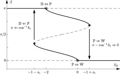
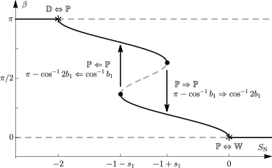
(a)	(b)
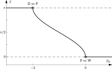
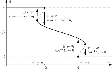
(c)	(d)

Figure 3: Summaries of the solutions for the contact angle $\displaystyle\beta$ as a function of the nematic spreading parameter $\displaystyle S_{\rm N}$ for NS-dominant anchoring according to 51 for the four ranges of $\displaystyle\Delta_{\rm GN}$: (a) $\displaystyle\Delta_{\rm GN}<-4$, (b) $\displaystyle-4\leq\Delta_{\rm GN}\leq-1$, (c) $\displaystyle-1\leq\Delta_{\rm GN}\leq 1/2$, and (d) $\displaystyle\Delta_{\rm GN}>1/2$. The transition points are labelled and shown by stars $\displaystyle(\mathop{\scalebox{1.5}{\raisebox{-0.86108pt}{$\displaystyle\ast$}}})$ for a continuous transition and by dots ($\displaystyle\bullet$) for a discontinuous transition, where $\displaystyle s_{1}=\sqrt{4(1+\Delta_{\rm GN})^{3}/(27\Delta_{\rm GN})}$, $\displaystyle b_{1}=\sqrt{(1+\Delta_{\rm GN})/(3\Delta_{\rm GN})}$ and $\displaystyle b_{2}=-1/2+\sqrt{\Delta_{\rm GN}(\Delta_{\rm GN}+4)}/(2\Delta_{\rm GN})$. The arrows shows the directions of the associated transitions in $\displaystyle\beta$. The solid lines denote the hypothesised local minimum energy states and the dashed lines denote the hypothesised local maximum energy states.

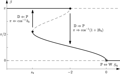
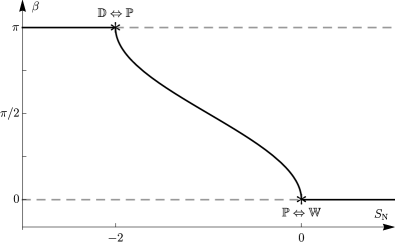
(a)	(b)
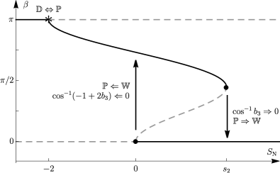
(c)

Figure 4: Summaries of the solutions for the contact angle $\displaystyle\beta$ as a function of the nematic spreading parameter $\displaystyle S_{\rm N}$ for GN-dominant anchoring according to 52 for the three ranges of $\displaystyle\Delta_{\rm NS}$: (a) $\displaystyle\Delta_{\rm NS}<-1/2$, (b) $\displaystyle-1/2\leq\Delta_{\rm NS}\leq 1/2$, and (c) $\displaystyle\Delta_{\rm NS}>1/2$. The transition points are labelled and shown by stars $\displaystyle(\mathop{\scalebox{1.5}{\raisebox{-0.86108pt}{$\displaystyle\ast$}}})$ for a continuous transition and by dots ($\displaystyle\bullet$) for a discontinuous transition, where $\displaystyle s_{2}=-1-\Delta_{\rm NS}-1/(4\Delta_{\rm NS})$ and $\displaystyle b_{3}=-1/(2\Delta_{\rm NS})$. The arrows shows the directions of the associated transitions in $\displaystyle\beta$. The solid lines denote the hypothesised local minimum energy states and the dashed lines denote the hypothesised local maximum energy states.

In Figures 3 and 4, and what follows, a rightward arrow ($\displaystyle\Rightarrow$) denotes a discontinuous transition for increasing $\displaystyle S_{\rm N}$, and a leftward arrow ($\displaystyle\Leftarrow$) denotes a discontinuous transition for decreasing $\displaystyle S_{\rm N}$. Thus, for example, a discontinuous transition from complete wetting to partial wetting for increasing $\displaystyle S_{\rm N}$ is denoted by $\displaystyle\mathbb{W}\Rightarrow\mathbb{P}$, and a discontinuous transition from partial wetting to complete wetting for decreasing $\displaystyle S_{\rm N}$ is denoted by $\displaystyle\mathbb{W}\Leftarrow\mathbb{P}$. In addition, we denote a discontinuous transition in the contact angle using the same notation, so that, for example, the contact-angle transition for a $\displaystyle\mathbb{W}\Rightarrow\mathbb{P}$ transition, for which the contact angle transitions discontinuously from $\displaystyle\beta=0$ to $\displaystyle\beta=\beta^{*}$, is denoted by $\displaystyle 0\Rightarrow\beta^{*}$. Summaries of all of the possible transitions shown in Figures 3 and 4 are given in Tables 1 and 2 for NS-dominant and GN-dominant anchoring, respectively.

Range of $\displaystyle\Delta_{\rm GN}$	$\displaystyle S_{\rm N}$ value at transition	Nature of the transition	Contact-angle transition
$\displaystyle\Delta_{\rm GN}<-4$	$\displaystyle-1-s_{1}\>(<-2)$	$\displaystyle\mathbb{D}\Leftarrow\mathbb{P}$	$\displaystyle\pi\Leftarrow\cos^{-1}b_{1}$
	$\displaystyle-2$	$\displaystyle\mathbb{D}\Leftrightarrow\mathbb{P}$	Continuous with $\displaystyle\beta=\pi$
	$\displaystyle 0$	$\displaystyle\mathbb{P}\Leftrightarrow\mathbb{W}$	Continuous with $\displaystyle\beta=0$
	$\displaystyle(0<)\,-1+s_{1}$	$\displaystyle\mathbb{P}\Rightarrow\mathbb{W}$	$\displaystyle\pi-\cos^{-1}b_{1}\Rightarrow 0$
$\displaystyle-4\leq\Delta_{\rm GN}<-1$	$\displaystyle-2$	$\displaystyle\mathbb{D}\Leftrightarrow\mathbb{P}$	Continuous with $\displaystyle\beta=\pi$
	$\displaystyle(-2\leq)\,-1-s_{1}\,(<-1)$	$\displaystyle\mathbb{P}\Leftarrow\mathbb{P}$	$\displaystyle\pi-\cos^{-1}2b_{1}\Leftarrow\cos^{-1}b_{1}$
	$\displaystyle(-1<)\,-1+s_{1}\,(\leq 0)$	$\displaystyle\mathbb{P}\Rightarrow\mathbb{P}$	$\displaystyle\pi-\cos^{-1}b_{1}\Rightarrow\cos^{-1}2b_{1}$
	$\displaystyle 0$	$\displaystyle\mathbb{P}\Leftrightarrow\mathbb{W}$	Continuous with $\displaystyle\beta=0$
$\displaystyle-1\leq\Delta_{\rm GN}\leq 1/2$	$\displaystyle-2$	$\displaystyle\mathbb{D}\Leftrightarrow\mathbb{P}$	Continuous with $\displaystyle\beta=\pi$
	$\displaystyle 0$	$\displaystyle\mathbb{P}\Leftrightarrow\mathbb{W}$	Continuous with $\displaystyle\beta=0$
$\displaystyle\Delta_{\rm GN}>1/2$	$\displaystyle-1-s_{1}\,(<-2)$	$\displaystyle\mathbb{D}\Leftarrow\mathbb{P}$	$\displaystyle\pi\Leftarrow\pi-\cos^{-1}b_{1}$
	$\displaystyle-2$	$\displaystyle\mathbb{D}\Rightarrow\mathbb{P}$	$\displaystyle\pi\Rightarrow\pi-\cos^{-1}b_{2}$
	$\displaystyle 0$	$\displaystyle\mathbb{P}\Leftarrow\mathbb{W}$	$\displaystyle\cos^{-1}b_{2}\Leftarrow 0$
	$\displaystyle(0<)\,-1+s_{1}$	$\displaystyle\mathbb{P}\Rightarrow\mathbb{W}$	$\displaystyle\cos^{-1}b_{1}\Rightarrow 0$

Table 1: Summary of all of the possible transitions for NS-dominant anchoring obtained from 51. The four ranges of values of $\displaystyle\Delta_{\rm GN}$, the $\displaystyle S_{\rm N}$ value at which transitions occur, where $\displaystyle s_{1}=\sqrt{4(1+\Delta_{\rm GN})^{3}/(27\Delta_{\rm GN})}$, and the nature of the different transitions and the contact-angle transitions, where $\displaystyle b_{1}=\sqrt{(1+\Delta_{\rm GN})/(3\Delta_{\rm GN})}$ and $\displaystyle b_{2}=-1/2+\sqrt{\Delta_{\rm GN}(\Delta_{\rm GN}+4)}/(2\Delta_{\rm GN})$, are shown.

Range of $\displaystyle\Delta_{\rm NS}$	$\displaystyle S_{\rm N}$ value at transition	Nature of the transition	Contact-angle transition
$\displaystyle\Delta_{\rm NS}<-1/2$	$\displaystyle-2$	$\displaystyle\mathbb{D}\Leftrightarrow\mathbb{P}$	Continuous with $\displaystyle\beta=\pi$
	$\displaystyle 0$	$\displaystyle\mathbb{P}\Leftarrow\mathbb{W}$	$\displaystyle\cos^{-1}\left(-1+2b_{3}\right)\Leftarrow 0$
	$\displaystyle(0<)\,s_{2}$	$\displaystyle\mathbb{P}\Rightarrow\mathbb{W}$	$\displaystyle\cos^{-1}b_{3}\Rightarrow 0$
$\displaystyle-1/2\leq\Delta_{\rm NS}\leq 1/2$	$\displaystyle-2$	$\displaystyle\mathbb{D}\Leftrightarrow\mathbb{P}$	Continuous with $\displaystyle\beta=\pi$
	$\displaystyle 0$	$\displaystyle\mathbb{P}\Leftrightarrow\mathbb{W}$	Continuous with $\displaystyle\beta=0$
$\displaystyle\Delta_{\rm NS}>1/2$	$\displaystyle s_{2}\,(<-2)$	$\displaystyle\mathbb{D}\Leftarrow\mathbb{P}$	$\displaystyle\pi\Leftarrow\cos^{-1}b_{3}$
	$\displaystyle-2$	$\displaystyle\mathbb{D}\Rightarrow\mathbb{P}$	$\displaystyle\pi\Rightarrow\cos^{-1}\left(1+2b_{3}\right)$
	$\displaystyle 0$	$\displaystyle\mathbb{P}\Leftrightarrow\mathbb{W}$	Continuous with $\displaystyle\beta=0$

Table 2: Summary of all of the possible transitions for GN-dominant anchoring obtained from 52. The three ranges of values of $\displaystyle\Delta_{\rm GN}$, the $\displaystyle S_{\rm N}$ value at which transitions occur, where $\displaystyle s_{2}=-1-\Delta_{\rm NS}-1/(4\Delta_{\rm NS})$, and the nature of the different transitions and the contact-angle transitions, where $\displaystyle b_{3}=-1/(2\Delta_{\rm NS})$, are shown.

Although for a nematic ridge, unlike for an isotropic ridge, the free energy of each equilibrium state cannot be determined analytically, we can hypothesise the local minimum energy states for the nematic ridge by comparison with those for the isotropic ridge described in Section 5. Hence we hypothesise that the $\displaystyle\mathbb{D}$ state is a local minimum energy state for $\displaystyle S_{\rm N}<-2$ and a local maximum energy state for $\displaystyle S_{\rm N}\geq-2$. Similarly, we hypothesise that the $\displaystyle\mathbb{W}$ state is a local minimum energy state for $\displaystyle S_{\rm N}>0$ and a local maximum energy state for $\displaystyle S_{\rm N}\leq 0$. Assuming that there will always be at least one local minimum energy state, within the range $\displaystyle-2\leq S_{\rm N}\leq 0$, where the $\displaystyle\mathbb{W}$ and the $\displaystyle\mathbb{D}$ states are local maximum energy states, the local minimum energy state must be a $\displaystyle\mathbb{P}$ state. The local minimum and maximum energy states are shown in Figures 3 and 4 by solid lines and dashed lines, respectively. In the absence of a full dynamical theory, we also hypothesise that the continuous and discontinuous transitions shown in Figures 3 and 4 each correspond to classical pitchfork or fold bifurcations [57]. In particular, the transitions at $\displaystyle S_{\rm N}=-2$ and $\displaystyle S_{\rm N}=0$ are pitchfork bifurcations, where a change in $\displaystyle S_{\rm N}$, $\displaystyle\Delta_{\rm GN}$ or $\displaystyle\Delta_{\rm NS}$ leads to a local minimum energy state becoming a local maximum energy state, forcing the system to transition continuously (through a super-critical pitchfork bifurcation) or discontinuously (through a sub-critical pitchfork bifurcation) to a new local minimum energy state. Furthermore, the discontinuous transitions at $\displaystyle S_{\rm N}=-1\pm s_{1}$ and $\displaystyle S_{\rm N}=s_{2}$, where

$$\displaystyle s_{1} \displaystyle=\sqrt{4(1+\Delta_{\rm GN})^{3}/(27\Delta_{\rm GN})},$$ (56)

$$\displaystyle s_{2} \displaystyle=-1-\Delta_{\rm NS}-1/(2\Delta_{\rm NS}),$$ (57)

are associated with fold bifurcations, where a change in $\displaystyle S_{\rm N}$, $\displaystyle\Delta_{\rm GN}$ or $\displaystyle\Delta_{\rm NS}$ leads to a local minimum energy state combining with a local maximum energy state, forcing the system to transition discontinuously to a different local minimum energy state.

Figures 3(a) and (b) and Figures 4(a) and (c) also show that there are ranges of $\displaystyle S_{\rm N}$ values for which there are two local minimum energy states (shown by solid lines). Perhaps most interestingly, we see from Figure 3(a) that when $\displaystyle-2\leq S_{\rm N}\leq 0$ and from Figure 3(b) that when $\displaystyle-1-s_{1}\leq S_{\rm N}\leq-2$ there are two local minimum energy $\displaystyle\mathbb{P}$ states. This implies that the effects of anchoring breaking can give rise to two local minimum energy $\displaystyle\mathbb{P}$ states, a situation that does not occur in the isotropic case.

From the results summarised in Tables 2 and 1 the asymptotic behaviour of the contact-angle transitions in the limits of large anchoring coefficients relative to the isotropic interfacial tension, namely the limits $\displaystyle\Delta_{\rm GN}\to\pm\infty$ and $\displaystyle\Delta_{\rm NS}\to\pm\infty$, may be determined. For example, for NS-dominant anchoring, as $\displaystyle\Delta_{\rm GN}\to\infty$ the contact-angle transition for the $\displaystyle\mathbb{P}\Leftarrow\mathbb{W}$ transition approaches a discontinuous transition in contact angle from $\displaystyle\beta=0$ to $\displaystyle\beta=\pi/2$, and the contact-angle transition for the $\displaystyle\mathbb{D}\Rightarrow\mathbb{P}$ transition approaches a discontinuous transition in the contact angle from $\displaystyle\beta=\pi$ to $\displaystyle\beta=\pi/2$. This limiting behaviour shows that for GN-dominant anchoring in the limit $\displaystyle\Delta_{\rm NS}\to\infty$ the contact-angle transition for the $\displaystyle\mathbb{P}\Leftarrow\mathbb{W}$ transition approaches a discontinuous transition in the contact angle from $\displaystyle\beta=0$ to $\displaystyle\beta=\pi$, i.e. it approaches a discontinuous transition from the $\displaystyle\mathbb{W}$ state directly to the $\displaystyle\mathbb{D}$ state, which bypasses the $\displaystyle\mathbb{P}$ state. Similarly, in the limit $\displaystyle\Delta_{\rm NS}\to-\infty$ the contact-angle transition for the $\displaystyle\mathbb{D}\Rightarrow\mathbb{P}$ transition approaches a discontinuous transition in the contact angle from $\displaystyle\beta=\pi$ to $\displaystyle\beta=0$, i.e. it approaches a discontinuous transition from the $\displaystyle\mathbb{D}$ state directly to the $\displaystyle\mathbb{W}$ state.

The discontinuous transitions shown in Figures 3(a), (b), and (d) and Figures 4(a) and (c) show that the behaviour of the contact angle is hysteretic. This nematic contact-angle hysteresis, which occurs for an ideal substrate, is fundamentally different from the well-known phenomenon of isotropic contact-angle hysteresis which, as we have previously mentioned, occurs only for a non-ideal substrate. However, we note that when $\displaystyle-1\leq\Delta_{\rm GN}\leq 1/2$ for NS-dominant anchoring, as shown in Figure 3(c), and when $\displaystyle-1/2\leq\Delta_{\rm NS}\leq 1/2$ for GN-dominant anchoring, as shown in Figure 4(b), the behaviour is similar to the isotropic case and no contact-angle hysteresis occurs.

8 Conclusions

In the present work we analysed a two-dimensional static ridge of nematic resting on an ideal solid substrate in an atmosphere of passive gas. In Sections 2 and 3, we obtained the first complete theoretical description for this system by minimising the free energy, which is given by the sum of the bulk elastic energy, gravitational potential energy and the interface energies, subject to a prescribed constant cross-sectional area. We then, in Section 4, chose explicit forms of the bulk elastic energy density and the interface energy densities, namely the standard Oseen–Frank bulk elastic energy density and the standard Rapini–Papoular interface energy densities, and obtained the governing equations 38, 39, 40, 4.2, 42 and 43. Specifically, these equations determine the director angle $\displaystyle\theta(x,z)$, the ridge height $\displaystyle h(x)$, the contact line positions $\displaystyle x=d^{\pm}$, and the Lagrange multiplier $\displaystyle p_{0}$, in terms of the physical parameters, namely the splay and bend elastic constants $\displaystyle K_{1}$ and $\displaystyle K_{3}$, the corresponding isotropic interfacial tensions $\displaystyle\gamma_{\rm GN}$, $\displaystyle\gamma_{\rm NS}$ and $\displaystyle\gamma_{\rm GS}$, and the anchoring strengths $\displaystyle C_{\rm GN}$ and $\displaystyle C_{\rm NS}$. These governing equations can, in principle, be generalised to include electromagnetic forces, additional contact line effects, non-ideal substrates, or more detailed models for the nematic molecular order, such as Q-tensor theory [58].

After briefly reviewing the behaviour of an isotropic ridge in Section 5 and discussing the nematic Young equations 42 and 43 in Section 6, in Section 7, under the assumption that anchoring breaking occurs in regions adjacent to the contact lines, we used the nematic Young equations 42 and 43 to determine the continuous and discontinuous transitions that occur between the $\displaystyle\mathbb{W}$, $\displaystyle\mathbb{P}$ and $\displaystyle\mathbb{D}$ states. In particular, it was shown that the nematic Young equations in the cases of NS-dominant and GN-dominant anchoring, which are given by 51 and 52, respectively, can each be written in terms of two parameters, namely the nematic spreading parameter $\displaystyle S_{\rm N}$ and one of the scaled anchoring coefficients $\displaystyle\Delta_{\rm GN}$ and $\displaystyle\Delta_{\rm NS}$. In both situations, we found continuous transitions analogous to those that occur in the classical case of an isotropic liquid, but also a variety of discontinuous transitions, as well as contact-angle hysteresis, and regions of parameter space in which there exist multiple partial wetting states that do not occur in the classical case of an isotropic liquid. Summaries of all the transitions for NS-dominant and GN-dominant anchoring are given in Figures 3 and 4, respectively, and in Tables 1 and 2, respectively.

For simplicity, in Section 7 we considered only the left-hand contact line, which is described by the nematic Young equation 42. Corresponding results can be obtained for the right-hand contact line, and, since we have shown that there is more than one possible contact angle value for the same parameter values, $\displaystyle\beta^{\pm}$ do not, in general, have to be the same and so the ridge can be asymmetric. This is in agreement with observations by Vanzo et al. [59], who found that anisotropic effects can lead to multiple contact-angle values and asymmetry of elongated sessile nematic droplets.

Concerning potential future comparisons with the results of physical experiments of the situation modelled in the present work, we have shown that discontinuous transitions and contact-angle hysteresis will occur if the parameters are such that $\displaystyle\Delta_{\rm GN}>1/2$ or $\displaystyle\Delta_{\rm GN}<-1$, or $\displaystyle|\Delta_{\rm NS}|>1/2$. Inspection of 55 and 54 shows that one of these inequalities may be satisfied when the isotropic interfacial tension and the anchoring strength are of similar magnitude at one of the interfaces, i.e. $\displaystyle\gamma_{\rm GN}\simeq|C_{\rm GN}|$ or $\displaystyle\gamma_{\rm NS}\simeq|C_{\rm NS}|$. For standard low-molecular-mass nematics, for which the isotropic interfacial tension is typically larger than the anchoring strength [7], this may be difficult to achieve. For example, for the typical parameter values given in Section 4, $\displaystyle|\Delta_{\rm GN}|\ll 1$ and $\displaystyle|\Delta_{\rm NS}|\ll 1$. Therefore, the present analysis indicates that, as many previous authors have implicitly or explicitly assumed, for standard low-molecular-mass nematics the classical isotropic Young equations 44 are a good approximation for the nematic Young equations 42 and 43 and discontinuous transitions and contact-angle hysteresis will not be observed. However, for high-molecular-mass nematics, e.g. nematic polymers, or systems with particularly strong anchoring, the anchoring strengths would be considerably higher, and the discontinuous transitions could potentially be observed experimentally. For example, the use of polymeric compounds to produce tailored anchoring [31] leads to a strong preference for polymers to align at interfaces [60, 61] and may result in large anchoring strengths, which could lead to $\displaystyle|\Delta_{\rm GN}|=O(1)$ and $\displaystyle|\Delta_{\rm NS}|=O(1)$ and hence the transitions predicted in the present work could potentially be observed. Alternatively, the situation in which the surrounding fluid is the isotropic melt of the nematic could lower the isotropic interfacial tension $\displaystyle\gamma_{\rm GN}$. In this situation, the isotropic interfacial tension for the isotropic–nematic interface $\displaystyle\gamma_{\rm IN}$ would be much smaller than the gas–nematic interfacial tension $\displaystyle\gamma_{\rm GN}$ and may become comparable with the anchoring strength $\displaystyle C_{\rm GN}$. For instance, $\displaystyle\gamma_{\rm IN}$ was measured for the nematic MBBA as $\displaystyle\gamma_{\rm IN}=10^{-5}\,{\rm Nm}^{-1}$ [62], which is three orders of magnitude smaller than typical isotropic interfacial tension for a gas–nematic interface $\displaystyle\gamma_{\rm GN}$ [54]. Such a situation could be realised experimentally by using controlled heating and cooling of regions of a substrate coated in a nematic film [31, 63].

The range of anisotropic wetting and dewetting phenomena occurring in this nematic system may also be useful from a technological perspective, for instance, for tailored dewetting of liquid films, as discussed in Section 1 [2, 18, 6, 41, 42]. The variety of possible transitions between two-dimensional equilibrium states will have similar forms in three dimensions, which may be relevant to applications such as the One Drop Filling method of LCD manufacturing [64, 65, 66] and adaptive-lens technologies [4, 5]. In order to explore such applications, further theoretical investigations, particularly into the dynamics of transitions, and experimental investigations would be needed.

References

- [1] J. Chen, W. Cranton, and M. Fihn, editors. Handbook of Visual Display Technology. Springer, 2012.
- [2] D. Gentili, G. Foschi, F. Valle, M. Cavallini, and F. Biscarini. Applications of dewetting in micro and nanotechnology. Chemical Society Reviews, 41(12):4430–4443, 2012.
- [3] A. Sengupta, U. Tkalec, M. Ravnik, J. M. Yeomans, C. Bahr, and S. Herminghaus. Liquid crystal microfluidics for tunable flow shaping. Physical Review Letters, 110(4):048303, 2013.
- [4] J. F. Algorri, D. C. Zografopoulos, V. Urruchi, and J. M. Sánchez-Pena. Recent advances in adaptive liquid crystal lenses. Crystals, 9(5):272, 2019.
- [5] S.-U. Kim, J.-H. Na, C. Kim, and S.-D. Lee. Design and fabrication of liquid crystal-based lenses. Liquid Crystals, 44(12–13):2121–2132, 2017.
- [6] C. Zou, J. Wang, M. Wang, Y. Wu, K. Gu, Z. Shen, G. Xiong, H. Yang, L. Jiang, and T. Ikeda. Patterning of discotic liquid crystals with tunable molecular orientation for electronic applications. Small, 14(21):1800557, 2018.
- [7] A. A. Sonin. The Surface Physics of Liquid Crystals. Gordon & Breach Science Publishers, 1995.
- [8] M.-A. Y.-H. Lam, L. Kondic, and L. J. Cummings. Effects of spatially-varying substrate anchoring on instabilities and dewetting of thin nematic liquid crystal films. Soft Matter, 16(44):10187–10197, 2020.
- [9] M.-A. Y.-H. Lam, L. J. Cummings, and L. Kondic. Stability of thin fluid films characterised by a complex form of effective disjoining pressure. Journal of Fluid Mechanics, 841:925–961, 2018.
- [10] T.-S. Lin, L. J. Cummings, A. J. Archer, L. Kondic, and U. Thiele. Note on the hydrodynamic description of thin nematic films: strong anchoring model. Physics of Fluids, 25(8):082102, 2013.
- [11] T.-S. Lin, L. Kondic, U. Thiele, and L. J. Cummings. Modelling spreading dynamics of nematic liquid crystals in three spatial dimensions. Journal of Fluid Mechanics, 729:214–230, 2013.
- [12] F. N. Braun and H. Yokoyama. Spinodal dewetting of a nematic liquid crystal film. Physical Review E, 62(2):2974–2976, 2000.
- [13] F. Vandenbrouck, M. P. Valignat, and A. M. Cazabat. Thin nematic films: metastability and spinodal dewetting. Physical Review Letters, 82(13):2693–2696, 1999.
- [14] O. V. Manyuhina. Shaping thin nematic films with competing boundary conditions. European Physical Journal E, 37(48):48–52, 2014.
- [15] P. G. de Gennes, F. Brochard-Wyart, and D. Quéré. Capillarity and Wetting Phenomena. Springer, 2004.
- [16] C. W. Extrand. Origins of wetting. Langmuir, 32(31):7697–7706, 2016.
- [17] A. L. Demirel and B. Jérôme. Restructuring-induced dewetting and re-entrant wetting of thin glassy films. Europhysics Letters, 45(1):58–64, 1999.
- [18] J. P. Bramble, D. J. Tate, D. J. Revill, K. H. Sheikh, J. R. Henderson, F. Liu, X. Zeng, G. Ungar, R. J. Bushby, and S. D. Evans. Planar alignment of columnar discotic liquid crystals by isotropic phase dewetting on chemically patterned surfaces. Advanced Functional Materials, 20(6):914–920, 2010.
- [19] I. W. Stewart. The Static and Dynamic Continuum Theory of Liquid Crystals. Taylor & Francis, 2004.
- [20] B. I. Ostrovskii, D. Sentenac, I. I. Samoilenko, and W. H. de Jeu. Structure and frustration in liquid crystalline polyacrylates II. Thin-film properties. The European Physical Journal E, 6(4):287–294, 2001.
- [21] D. van Effenterre and M. P. Valignat. Stability of thin nematic films. The European Physical Journal E, 12(3):367–372, 2003.
- [22] A. B. E. Vix, P Müller-Buschbaum, W. Stocker, M. Stamm, and J. P. Rabe. Crossover between dewetting and stabilization of ultrathin liquid crystalline polymer films. Langmuir, 16(26):10456–10462, 2000.
- [23] S. Herminghaus, K. Jacobs, K. Mecke, J. Bischof, A. Fery, M. Ibn-Elhaj, and S. Schlagowski. Spinodal dewetting in liquid crystal and liquid metal films. Science, 282(5390):916–919, 1998.
- [24] B. Ravi, R. Mukherjee, and D. Bandyopadhyay. Solvent vapour mediated spontaneous healing of self-organized defects of liquid crystal films. Soft Matter, 11(1):139–146, 2015.
- [25] C. Poulard and A. M. Cazabat. Spontaneous spreading of nematic liquid crystals. Langmuir, 21(14):6270–6276, 2005.
- [26] U. Delabre, C. Richard, and A. M. Cazabat. Thin nematic films on liquid substrates. The Journal of Physical Chemistry B, 113(12):3647–3652, 2009.
- [27] A. D. Rey and E. E. Herrera-Valencia. Dynamic wetting model for the isotropic-to-nematic transition over a flat substrate. Soft Matter, 10(10):1611–1620, 2014.
- [28] H. Yokoyama, S. Kobayashi, and H. Kamei. Deformations of a planar nematic-isotropic interface in uniform and nonuniform electric fields. Molecular Crystals and Liquid Crystals, 129(1–3):109–126, 1985.
- [29] E. Schäffer, T. Thurn-Albrecht, T. P. Russell, and U. Steiner. Electrically induced structure formation and pattern transfer. Nature, 403(6772):874–877, 2000.
- [30] P. Oswald. Elasto- and electro-capillary instabilities of a nematic-isotropic interface: experimental results. The European Physical Journal E, 33(1):69–79, 2010.
- [31] M. W. J. van der Wielen, E. P. I. Baars, M. Giesbers, M. A. Cohen Stuart, and G. J. Fleer. The effect of substrate modification on the ordering and dewetting behavior of thin liquid-crystalline polymer films. Langmuir, 16(26):10137–10143, 2000.
- [32] O. D. Lavrentovich and V. M. Pergamenshchik. Stripe domain phase of a thin nematic film and the divergence term. Physical Review Letters, 73(7):979–982, 1994.
- [33] A. M. Cazabat, U. Delabre, C. Richard, and Y. Yip Cheung Sang. Experimental study of hybrid nematic wetting films. Advances in Colloid and Interface Science, 168(1–2):29–39, 2011.
- [34] J. T. Jenkins and P. J. Barratt. Interfacial effects in the static theory of nematic liquid crystals. Quarterly Journal of Mechanics and Applied Mathematics, 27(1):111–127, 1974.
- [35] G. Barbero and R. Barberi. Critical thickness of a hybrid aligned nematic liquid crystal cell. Journal de Physique, 44(5):609–616, 1983.
- [36] A. D. Rey. Nematostatics of triple lines. Physical Review E, 67(1):011706, 2003.
- [37] A. D. Rey. Capillary models for liquid crystal fibers, membranes, films, and drops. Soft Matter, 3(11):1349–1368, 2007.
- [38] N. Schopohl and T. J. Sluckin. Defect cores structure in nematic liquid crystals. Physical Review Letters, 59(22):2582–2584, 1987.
- [39] J. Walton, N. J. Mottram, and G. McKay. Nematic liquid crystal director structures in rectangular regions. Physical Review E, 97(2):022702, 2018.
- [40] S. Sergeyev, W. Pisula, and Y. H. Geerts. Discotic liquid crystals: a new generation of organic semiconductors. Chemical Society Reviews, 36(12):1902–1929, 2007.
- [41] M. L. Blow and M. M. Telo da Gama. Interfacial motion in flexo- and order-electric switching between nematic filled states. Journal of Physics: Condensed Matter, 25(24):245103, 2013.
- [42] C. V. Brown, G. G. Wells, M. I. Newton, and G. McHale. Voltage-programmable liquid optical interface. Nature Photonics, 3(7):403–405, 2009.
- [43] A. D. Rey. The Neumann and Young equations for nematic contact lines. Liquid Crystals, 27(2):195–200, 2000.
- [44] A. D. Rey. Young–Laplace equation for liquid crystal interfaces. The Journal of Chemical Physics, 113(23):10820–10822, 2000.
- [45] A. Rapini and M. Papoular. Distorsion d’une lamelle nématique sous champ magnétique conditions d’ancrage aux parois. Journal de Physique Colloque, 30(C4):C4–54–C4–56, 1969.
- [46] F. Mugele and J. Heikenfeld. Electrowetting: Fundamental Principles and Practical Applications. John Wiley & Sons, 2019.
- [47] J. R. L. Cousins. Mathematical Modelling and Analysis of Industrial Manufacturing of Liquid Crystal Displays. PhD thesis, University of Strathclyde, 2021.
- [48] N. J. Mottram and C. J. P. Newton. Liquid crystal theory and modelling. In J. Chen, W. Cranton, and M. Fihn, editors, Handbook of Visual Display Technology, chapter 7.2.3, pages 1403–1429. Springer, 2012.
- [49] H. Yokoyama and H. A. van Sprang. A novel method for determining the anchoring energy function at a nematic liquid crystal-wall interface from director distortions at high fields. Journal of Applied Physics, 57(10):4520–4526, 1985.
- [50] Yu. A. Nastishin, R. D. Polak, S. V. Shiyanovskii, V. H. Bodnar, and O. D. Lavrentovich. Nematic polar anchoring strength measured by electric field techniques. Journal of Applied Physics, 86(8):4199–4213, 1999.
- [51] H. Yokoyama. Surface anchoring of nematic liquid crystals. Molecular Crystals and Liquid Crystals, 165(1):265–316, 1988.
- [52] M. Slavinec, G. D. Crawford, S. Kralj, and S. Žumer. Determination of the nematic alignment and anchoring strength at the curved nematic–air interface. Journal of Applied Physics, 81(5):2153–2156, 1997.
- [53] R. Chiarelli, S. Faetti, and L. Fronzoni. Determination of the molecular orientation at the free surface of liquid crystals from Brewster angle measurements. Optics Communications, 46(1):9–13, 1983.
- [54] P. Dhara and R. Mukherjee. Influence of substrate surface properties on spin dewetting, texture and phase transition of 5CB liquid crystal thin film. Journal of Physical Chemistry B, 124(7):1293–1300, 2020.
- [55] M. Kléman. Points, Lines and Walls in Liquid Crystals, Magnetic Systems and Various Ordered Media. John & Wiley Sons, 1983.
- [56] M. K. McCamley, M. Ravnik, A. W. Artenstein, S. M. Opal, S. Žumer, and G. P. Crawford. Detection of alignment changes at the open surface of a confined nematic liquid crystal sensor. Journal of Applied Physics, 105(12):123504, 2009.
- [57] J. Guckenheimer and P. J. Holmes. Nonlinear Oscillations, Dynamical Systems, and Bifurcations of Vector Fields. Springer, 1983.
- [58] N. J. Mottram and C. J. P. Newton. Introduction to Q-tensor theory. arXiv preprint arXiv:1409.3542, 2014.
- [59] D. Vanzo, M. Ricci, R. Berardi, and C. Zannoni. Wetting behaviour and contact angles anisotropy of nematic nanodroplets on flat surfaces. Soft Matter, 12(5):1610–1620, 2016.
- [60] J. Zhou, D. M. Collard, J. O. Park, and M. Srinivasarao. Control of anchoring of nematic fluids at polymer surfaces created by in situ photopolymerization. The Journal of Physical Chemistry B, 109(18):8838–8844, 2005.
- [61] X. Li, T. Yanagimachi, C. Bishop, C. Smith, M. Dolejsi, H. Xie, K. Kurihara, and P. F. Nealey. Engineering the anchoring behavior of nematic liquid crystals on a solid surface by varying the density of liquid crystalline polymer brushes. Soft Matter, 14(37):7569–7577, 2018.
- [62] D. Langevin and M. A. Bouchiat. Molecular order and surface tension for the nematic-isotropic interface of MBBA, deduced from light reflectivity and light scattering measurements. Molecular Crystals and Liquid Crystals, 22(3–4):317–331, 1973.
- [63] P. Dhara and R. Mukherjee. Phase transition and dewetting of a 5CB liquid crystal thin film on a topographically patterned substrate. Royal Society of Chemistry Advances, 9(38):21685–21694, 2019.
- [64] J. R. L. Cousins, S. K. Wilson, N. J. Mottram, D. Wilkes, and L. Weegels. Squeezing a drop of nematic liquid crystal with strong elasticity effects. Physics of Fluids, 31(8):083107, 2019.
- [65] J. R. L. Cousins, S. K. Wilson, N. J. Mottram, D. Wilkes, and L. Weegels. Transient flow-driven distortion of a nematic liquid crystal in channel flow with dissipative weak planar anchoring. Physical Review E, 102(6):062703, 2020.
- [66] K.-C. Fan, J.-Y. Chen, C.-H. Wang, and W.-C. Pan. Development of a drop-on-demand droplet generator for one-drop-fill technology. Sensors and Actuators A: Physical, 147(2):649–655, 2008.