A posteriori error estimates for domain decomposition methods

Abstract.

Nowadays, a posteriori error control methods have formed a new important part of the numerical analysis. Their purpose is to obtain computable error estimates in various norms and error indicators that show distributions of global and local errors of a particular numerical solution.

In this paper, we focus on a particular class of domain decomposition methods (DDM), which are among the most efficient numerical methods for solving PDEs. We adapt functional type a posteriori error estimates and construct a special form of error majorant which allows efficient error control of approximations computed via these DDM by performing only subdomain-wise computations. The presented guaranteed error bounds use an extended set of admissible fluxes which arise naturally in DDM.

1. Introduction

1.1. Domain decomposition methods

The iteration method of Schwarz [37] suggested for analysis of conformal mappings has generated a branch of computational methods, which are nowadays among the most used in practice for the numerical solution of PDEs. In application to elliptic boundary value problems, proofs of convergence were first presented in the paper by S. Mikhlin [28] and in the book of Kantorovich and Krilov [9], implementation issues first discussed in [38].

The pioneering works on the Schwarz alternating method by Pierre-Louis Lions [17, 18, 19], Matsokin and Nepomnyaschikh [26, 27] provided the basis of the abstract Schwarz theory, for multiplicative methods see also [2], and herewith layed the foundations of modern domain decomposition methods (DDM). Schwarz methods exist as overlapping and non-overlapping methods, where representatives of either category can be formulated as additive or multiplicative subspace correction, as well as hybrid methods, see, e.g. [40].

Broad overviews and newer developments in the area of DDM were presented in [40, 25, 4]. Together with multigrid/algebraic multigrid (MG/AMG) methods, see, e.g., [8, 41, 42], DDM have become one of the most successful classes of iterative solution methods when it comes to cost- and energy-efficient computations of approximate solutions of PDEs. Their description and convergence analysis in the abstract framework of subspace correction (SSC) methods has been presented by Xu and Zikatanov [45].

There exist also hybrid approaches to construct solvers and preconditioners for a broad range of discrete models based on PDE. The idea to combine domain decomposition and multigrid techniques can be found as early as in [15]. The auxiliary space multigrid (ASMG) method presented in [13] implements this concept by means of auxiliary space preconditioning, see [44], and achieves herewith robustness with respect to general coefficient variations [14].

Nonoverlapping DDM or substructuring methods, as they are sometimes referred to, come as primal and dual methods. Balancing domain decomposition (BDD), see [21], is a primal method operating on the common interface degrees of freedom (DOF) whereas finite element tearing and interconnecting (FETI) enforces equality of DOF on substructure interfaces by Lagrange multipliers and thus is a dual method.

Nonoverlapping DDM, including BDDC (BDD based on constraints), see [3], and FETI-DP (FETI dual-primal), see [6], can be formulated and analyzed in a common algebraic framework, see [22, 23, 24]. The BDDC method enforces continuity across substructure interfaces by a certain averaging operator.

A key tool in the analysis of overlapping DD methods is the Poincaré inequality or its weighted analog as for problems with highly varying coefficients. It is well-known that the weighted Poincaré inequality holds only under certain conditions, e.g., in case of quasi-monotonic coefficients, see [35]. More recently the robustness of DD methods has also been achieved for problems with general coefficient variations using coarse spaces that are constructed by solving local generalized eigenvalue problems, see, e.g., [5, 7, 36].

The additional constraints can be viewed as subspace corrections involving the coarse basis functions, which are subject to energy minimization. From this point of view, the BDDC method [3] has also a high degree of similarity with the ASMG method [13]. However, contrary to BDDC, the latter, in general exploits overlapping subdomains where coarse DOF are associated not only with subdomain interfaces (or boundaries) but also with their interior. The recursive application of the two-level method then results in a full multilevel/multigrid algorithm. Its main characteristics are, contrary to standard (variational) multigrid algorithms, an auxiliary-space correction step instead of classical coarse-grid correction, and a coarse-grid operator arising from an additive approximation of the Schur complement of the original system, see also [11, 12].

The main advantage of domain decomposition methods is their ability to solve geometrically complicated problems by solving problems on simple subdomains. These methods have proven their high efficiency both for relatively simple cases where the number of subdomains is small (as in the left picture of Figure 1) and for engineering problems related to complicated 3D domains (right picture of Figure 1).

A posteriori error estimates are not only a key element of reliable computer simulations but are also well-suited to be combined and interact with modern SSC resulting in even more cost- and energy-efficient computational methods for PDEs.

Figure 1. Decomposition of two– and three–dimensional domains.

Our work is inspired by the idea to supply DDM with guaranteed error control following the guiding principle, namely, reducing the estimation of global errors to error estimates for subdomains.

1.2. Fully guaranteed a posteriori error estimates

Difficulties related to generation of fully computable, guaranteed, and consistent error bounds for partial differential equations are easy to explain with the paradigm of the simplest elliptic problem $\Delta u+f=0$ in a bounded Lipschitz domain $\Omega$ with the boundary condition $u=0$ on $\partial\Omega$. The solution $u$ is an element of the Sobolev space $H^{1}_{0}(\Omega)$ (that contains square integrable functions, which vanish on the boundary and have square integrable generalized derivatives of the first order). It is formally defined by the integral identity

(1) $$\int\limits_{\Omega}(\nabla u\cdot\nabla w-fw)dx=0\qquad\forall w\in H^{1}_{0}(\Omega).$$

Let $v\in H^{1}_{0}(\Omega)$ be an approximation of $u$ (e.g., computed by a Ritz-Galerkin finite element method). From (1), it follows that

(2) $$\int\limits_{\Omega}\nabla(u-v)\cdot\nabla wdx=\int\limits_{\Omega}(\nabla v\cdot\nabla w-fw)dx.$$

The right hand side of (2) can be estimated via the residual of the equation $R(v)=\Delta v+f$ in two ways. The first way is possible if $v$ has an extra regularity, so that $R(v)\in L^{2}(\Omega)$. Then we integrate by parts, use the Friedrichs inequality with a positive constant $C_{F}$ (which depends on $\Omega$) and arrive at the estimate

(3) $$\|\Delta(u-v)\|_{\Omega}\leq C_{F}\|\Delta v+f\|_{\Omega},$$

where $\|\cdot\|_{\Omega}$ stands for the norm of scalar and vector valued functions in $L^{2}(\Omega)$. Notice that the quantity in the left hand side of (2) can be considered as a measure of the error $e=u-v$. This quantity majorates $\|\nabla e\|$ with some constant multiplier (which for a convex domain $\Omega$ is equal to 1).

The right hand side of (3) is directly computable, so that at first glance the estimate looks attractive. However, from a computational point of view, this estimate has a fatal drawback: it is not applicable to a sequence of approximations $\{v_{k}\}$ converging to $u$ in the energy space $H^{1}_{0}(\Omega)$. Even if the sequence is regularized so that $R(v_{k})\in L^{2}(\Omega)$ and the norms in (3) are computable and finite for any $k$, we are unable to guarantee that the strong norm of the residual tends to zero. Hence, (3) does not possess an important consistency property.

Another way of error estimation operates with a weak norm of $R(v)$

(4) $$\sup\limits_{w\in H^{1}_{0}(\Omega)}\frac{\int\limits_{\Omega}\nabla(u-v)\cdot\nabla wdx}{\|\nabla w\|_{\Omega}}=\sup\limits_{w\in H^{1}_{0}(\Omega)}\frac{\int\limits_{\Omega}(\nabla v\cdot\nabla w-fw)dx}{\|\nabla w\|_{\Omega}}=:{\bm{|}\!\!\bm{|}\,}R(v){\bm{|}\!\!\bm{|}\,}_{-1,\Omega}.$$

It is easy to show that the left hand side of (4) coincides with $\|\nabla e\|_{\Omega}$. Moreover, the norm ${\bm{|}\!\!\bm{|}\,}R(v_{k}){\bm{|}\!\!\bm{|}\,}_{-1,\Omega}$ tends to zero if $v_{k}$ tends to $u$ in $H^{1}_{0}(\Omega)$ and, therefore, this error relation is consistent. But here we are faced with another difficulty. Unlike integral type norms, the norm ${\bm{|}\!\!\bm{|}\,}R(v){\bm{|}\!\!\bm{|}\,}_{-1,\Omega}$ is incomputable because the supremum is taken over an infinite amount of test functions. If the set of functions is reduced to some finite dimensional subspace, then the upper bound in (4) may be lost. An attempt to overcome this difficulty and get a computable majorant of ${\bm{|}\!\!\bm{|}\,}R(v){\bm{|}\!\!\bm{|}\,}_{-1,\Omega}$ using special properties of $v$ (Galerkin orthogonality) is known in the literature as the explicit residual method (e.g., see [43]). In practice, this way leads to the above discussed class of error indicators.

A posteriori error estimates, which are guaranteed, do not contain mesh–dependent constants, and are valid for any conforming approximation error, are derived by more sophisticated methods (see a consequent exposition in [34, 33, 20]). Estimates of this type are derived by purely functional methods without attraction of an information about the method and mesh used to compute a numerical solution. Therefore, they are known as a posteriori estimates of the functional type. These estimates do not use special properties of approximations (e.g., Galerkin orthogonality or superconvergence) as well as of the exact solution (additional regularity). The simplest estimate of this class for the problem (7a)–(7c) reads

(5) $$\|\nabla(u-v)\|_{A}\leq\|A\nabla v-\bm{y}\|_{A^{-1}}+C_{F}\|{\rm div}\bm{y}+f\|_{\Omega},$$

where $C_{F}$ is the constant in the Friedrichs inequality for the doman $\Omega$ and we use the notation

$$\|\bm{q}\|^{2}_{A}:=\int\limits_{\Omega}A\bm{q}\cdot\bm{q}dx\quad\text{and}\quad\|\bm{q}\|^{2}_{A^{-1}}:=\int\limits_{\Omega}A^{-1}\bm{q}\cdot\bm{q}dx\quad\forall\bm{q}\in[L^{2}(\Omega)]^{d}.$$

This estimate is valid for any function $v\in H^{1}(\Omega)$ that satisfies the boundary condition (7b) and any vector valued function $\bm{y}$ in the space

$$H(\Omega,{\rm div}):=\left\{\bm{q}\in[L^{2}(\Omega)]^{d}:\,{\rm div}\bm{q}\in L^{2}(\Omega)\right\}.$$

The function $\bm{y}$ can be viewed as an approximation of the exact flux $\bm{p}=A\nabla u$. It is easy to see that if $\bm{y}=\bm{p}$ then the estimate coincides with the exact error. If $\bm{q}\in Q_{f}$, see (10), then we arrive at the well known hypercircle estimate (see [39, 29])

(6) $$\|\nabla(u-v)\|_{A}\leq\inf_{\bm{q}\in Q_{f}}\|A\nabla v-\bm{q}\|_{A^{-1}}.$$

There is a whole class of a posteriori methods based on the use of (6) and its analogs for different boundary value problems. In them, $\bm{y}$ is defined by post–processing of the numerical flux $A\nabla v$ (which does not belong to $Q_{f}$) and the main efforts are focused on satisfying (6) (exactly or approximately). Here, we refer to [10, 16] and subsequent papers of many authors devoted to a posteriori methods based on equilibration of fluxes (e.g., see [1]). Numerical procedures used to construct a suitable equilibrated flux can be rather complicated, and, most importantly, they do not always guarantee that condition (6) is exactly satisfied. In the latter case, the estimate does not provide a guaranteed upper bound of the error, but usually serves as a good error indicator. It should be outlined that $Q_{f}$ is a rather narrow subset of $H(\Omega,{\rm div})$. The space $H(\Omega,{\rm div})$ admits simple conforming approximations that preserve the continuity of $\bm{y}\cdot n$ on interior boundaries (e.g., the so-called Raviart-Thomas elements). Therefore, a numerical flux $A\nabla v$ can be projected to $H(\Omega,{\rm div})$ by very simple post–processing procedures. Moreover, it is useful to make several iterations of minimization with respect to $\bm{y}$. After that the right hand side of (5) gives a good and fully guaranteed majorant of the error. In this paper, we show that this approach can be adapted to domain decomposition methods.

In conclusion of this overview, a few words should be said about reliable control of the accuracy of numerical solutions to integral equations. They arise in a number of important mathematical models, and in addition, there are methods for analyzing differential equations by reducing them to integral equations (e.g., Picard–Lindelöf method [31]). Fully guaranteed a posteriori error estimates for this class of problems are based upon the estimates derived by A. Ostrovskii for abstract iteration procedures [32]. The reader can find a systematic discussion of these questions in Chapter 6 of [20].

1.3. Outline of the paper and main results

The present paper presents a new methodological approach that allows to control global error resulting in the process of applying a DD method to solve iteratively an elliptic boundary-value problem, e.g. Problem (7a)–(7c), using only computations on subdomains, that is, utilizing operators which are defined and act locally, on subdomains, only. Consequently, any entirety of approximate solutions of subdomain problems yields explicit estimates of local (subdomain) errors as well as of the global error at any stage of the iterative process and thus gives a picture of the error contributions associated with individual subdomains.

The remainder of this paper is organized as follows. Section 2 contains the formulation of a simple elliptic model problem, introduces some notation, and recalls the basic structure of functional a posteriori error estimates for an elliptic model problem. Section 2 provides algorithmic details and summarizes some known facts about domain decomposition methods as they can be combined with local (subdomain-wise) a posteriori error estimation that will be analyzed hereafter in Section 3. The main theroretical result of this work is the a posteriori error estimate stated in Theorem 3.1, which is especially designed for domain decomposition methods. Finally, Section 4 discusses numerical results, which, on the one hand, support the theoretical estimates presented in Section 2, and, on the other hand, suggest strategies and possibilities to further refine the proposed approach.

2. Domain decomposition methods for the basic elliptic problem

In the next section, we discuss guaranteed and fully computable error estimates adapted to DDM using the following elliptic boundary-value problem

(7a) $${\rm div}\bm{p}+\,f=0~{}~{}~{}\text{in}~{}~{}\Omega,$$

(7b) $$\bm{p}=A\nabla u,$$

(7c) $$u=u_{g}\;\;\text{on}~{}~{}\Gamma=\partial{\Omega},$$

where $\Omega\in{\rm I\!R}^{d}$ is a polygonal domain, $u_{g}$ is a given function in $H^{1}(\Omega)$, and (7c) is understood as equality of the corresponding traces.

We assume that $A$ is a symmetric positive definite (SPD) $d{\times}d$ matrix, satisfying the estimate

(8) $$C_{\min}\|\xi\|^{2}\leq A\xi\cdot\xi\leq C_{\max}\|\xi\|^{2},\quad\forall\xi\in{\rm I\!R}^{d}.$$

The corresponding weak formulation of the problem reads: find $u\in H^{1}_{0}(\Omega)$ such that

(9) $$a(u,w):=\int_{\Omega}A\nabla u\cdot\nabla w\,dx=\int_{\Omega}fw\,dx,\ \forall w\in V_{0}:=H^{1}_{0}(\Omega).$$

Hence the exact flux $\bm{p}=A\nabla u\in Q_{f}$, where

(10) $$Q_{f}:=\left\{\bm{q}\in[L^{2}(\Omega)]^{d}:\int_{\Omega}\bm{q}\cdot\nabla w=\int_{\Omega}fw\,dx\quad\forall\ w\in V_{0}\right\}.$$

The iterative solvers we study here fall into the category of alternating Schwarz type methods based on an overlapping domain decomposition. In order to describe the basic setting of such methods formally we use the following assumptions and notation.

Let $\Omega$ be partitioned into a collection of ”basic” (relatively simple, convex) subdomains ${{\omega}}_{k}$ (e.g., triangles or quadrilaterals for $d=2$ and tetrahedra or hexahedra for $d=3$) so that

(11) $$\overline{\Omega}=\bigcup_{k=1}^{N}\overline{{{\omega}}}_{k}\qquad{\rm and}\quad{{{\omega}}}_{i}\cap{{{\omega}}}_{j}=\emptyset\;{\rm if}\;i\neq j.$$

In addition to $\{{{\omega}}_{k}\}$, we consider another set of Lipschitz subdomains $\Omega_{j}$, $j=1,2,\ldots,M$ that are utilized by a domain decomposition method. For the decomposition of $\Omega$ into $\{\Omega_{j}:j=1,2,\ldots,M\}$ we assume that

(12) $$\overline{\Omega}=\bigcup_{j=1}^{M}\overline{\Omega}_{j},$$

and

(13) $$\overline{\Omega_{k}\cap\Omega_{l}}=\begin{cases}\emptyset,\\ \text{certain collection of }\overline{{{\omega}}}_{i},\end{cases}$$

which implies that each subdomain $\Omega_{j}$ itself is partitioned into a certain set of basic subdomains, i.e.,

(14) $$\overline{\Omega}_{k}=\bigcup_{j\in\mathcal{I}_{k}}\overline{{{\omega}}}_{j},$$

where $\mathcal{I}_{k}$ denotes the index set corresponding to the nonoverlapping partitioning of the subdomain $\Omega_{k}$ into basic subdomains ${{\omega}}_{j}$. Note that this setting allows to consider both overlapping and nonovelapping domain decomposition methods.

First, let $\gamma_{ji}=\gamma_{ij}$ denote the interface of $\overline{{{\omega}}}_{i}$ and $\overline{{{\omega}}}_{j}$, that is,

$$\gamma_{ij}:=\overline{{{\omega}}}_{i}\cap\overline{{{\omega}}}_{j}.$$

We assume that $\gamma_{ij}$ has a positive surface measure, otherwise ${{{\omega}}}_{i}$ and ${{{\omega}}}_{j}$ are considered as non–intersecting cells. Next, the boundary faces (edges) $\gamma_{i}$ of $\overline{{{\omega}}}_{i}$ are denoted by

$$\gamma_{i}:=\overline{{{\omega}}}_{i}\cap\Gamma.$$

Like this the boundary $\partial\Omega_{k}$ is given by

$$\partial\Omega_{k}:=\left(\bigcup_{i\in\mathcal{I}_{k}\land j\notin\mathcal{I}_{k}\lor i\notin\mathcal{I}_{k}\land j\in\mathcal{I}_{k}}\gamma_{ij}\right)\cup\left(\bigcup_{j\in\mathcal{I}_{k}}\gamma_{j}\right)=:\left(\bigcup_{i\notin\mathcal{I}_{k}}\Gamma_{k,i}\right)\cup\Gamma_{k}$$

and $\Gamma_{k}=\partial\Omega_{k}\cap\Gamma$. We will consider here the “overlapping case”, that is, the case in which $\gamma_{ij}\subset\partial\Omega_{k}$ for $i\in\mathcal{I}_{k}$ and $j\notin\mathcal{I}_{k}$ or $i\notin\mathcal{I}_{k}$ and $j\in\mathcal{I}_{k}$ implies that there exists $\Omega_{\ell}$ such that $i\in\mathcal{I}_{\ell}$ and $j\in\mathcal{I}_{\ell}$. Note that we do not care about the order of the indices $i$ and $j$ in $\gamma_{ij}$, that is, $\gamma_{ij}$ is identified with $\gamma_{ji}$ so that for “$i\in\mathcal{I}_{k}\land j\notin\mathcal{I}_{k}\lor i\notin\mathcal{I}_{k}\land j\in\mathcal{I}_{k}$” we could equivalently write “$i\notin\mathcal{I}_{k}\land j\in\mathcal{I}_{k}$”, for example. Figure 2 illustrates the notation we are using on a very simple example. The left picture shows two overlapping subdomains $\Omega_{1}$ and $\Omega_{2}$, which are composed of two basic subdomains each, i.e., $\overline{\Omega}_{1}=\overline{{{\omega}}}_{1}\cup\overline{{{\omega}}}_{2}$, $\overline{\Omega}_{2}=\overline{{{\omega}}}_{2}\cup\overline{{{\omega}}}_{3}$. Their intersection is given by $\Omega_{1}\cap\Omega_{2}={{\omega}}_{2}$. The right picture illustrates the three non-overlapping basic subdomains ${{\omega}}_{1}$, ${{\omega}}_{2}$, and ${{\omega}}_{3}$. The boundaries of $\Omega_{1}$ and $\Omega_{2}$ in this case are given by $\partial\Omega_{1}=\Gamma_{1,3}\cup\Gamma_{1}$ with $\Gamma_{1,3}=\gamma_{32}$ and $\Gamma_{1}=\gamma_{1}\cup\gamma_{2}$ and $\partial\Omega_{2}=\Gamma_{2,1}\cup\Gamma_{2}$ with $\Gamma_{2,1}=\gamma_{12}$ and $\Gamma_{2}=\gamma_{2}\cup\gamma_{3}$.

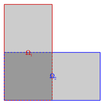
(a) Two overlapping subdomains $\Omega_{1}$ (vertically elongated rectangle) and $\Omega_{2}$ (horizontally elongated rectangle)

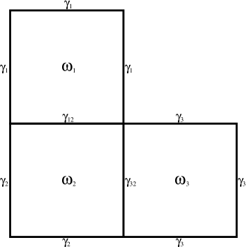
(b) Three non-overlapping basic subdomains ${{\omega}}_{1}$, ${{\omega}}_{2}$, and ${{\omega}}_{3}$

Figure 2. Notation for subdomains and boundaries

There are various ways to extend the classical Schwarz alternating method from two to more than two (overlapping) subdomains. We follow reference [18] and denote by $V_{k}$ the closed subspace of $H_{0}^{1}(\Omega)$ consisting of all elements of $H_{0}^{1}(\Omega_{k})$ extended by $0$ to $\Omega$.

Then we choose some initial guess $u_{0}^{1}\in H_{0}^{1}(\Omega)$ for the solution $u$ of problem  (7a)–(7c). Without loss of generality, we may assume that $g=0$, which we can always achieve by subtracting from the solution of the inhomogeneous equation a known function $u_{g}\in H^{1}(\Omega)$ satisfying the boundary condition $u_{g}=g$ on $\Gamma$ and modifying the right hand side of equation (7a) accordingly.

We use the following domain decomposition algorithm for solving the problem (7), see [18]:

Algorithm 2.1.

Choose initial guess $u_{0}^{1}\in H_{0}^{1}(\Omega)$
for n=1,2,...
	for k=1 to M
		Solve

(15a) $$-{\rm div}A\nabla u_{k}^{n} = f~{}~{}~{}~{}\text{in}\;\;\;\Omega_{k},\hskip 56.9055pt$$

(15b) $$u_{k}^{n} = u_{k-1}^{n}\;\;\text{on }~{}~{}~{}\partial{\Omega}_{k},$$

Extend

(15c) $$u_{k}^{n}\ \ \verb!to!\ \ \Omega\ \ \verb!by!\ \ u_{k-1}^{n}$$

The above algorithm is the classical Schwarz alternating method, which is a multiplicative Schwarz (successive subspace correction) method with an error propagation operator (see [40])

(16) $$E_{\rm{mu}}=(I-P_{M})(I-P_{M-1})\ldots(I-P_{1}),$$

where $P_{k}=R_{k}^{T}\widetilde{P}_{k}$ and $\widetilde{P}_{k}:V\rightarrow V_{k}$ are defined by

$$a_{k}(\widetilde{P}_{k}u,v_{k})=a(u,R_{k}^{T}v_{k})\quad\text{for all }v_{k}\in V_{k},\,k=1,\ldots,M.$$

Here $V\subset H_{0}^{1}(\Omega)$ is a finite dimensional approximation space, e.g., conforming finite element space, that is used to discretize the global problem (9) whereas $V_{k}$ denote corresponding spaces of functions with local support $\bar{\Omega}_{k}$ in which the solutions $u_{k}$ of the subdomain problems

(17) $$\begin{array}[]{rcl}a_{k}(u_{k},v_{k})&:=&\int_{\Omega_{k}}(A\nabla u_{k})\cdot\nabla v_{k}\,dx\\ &=&\int_{\Omega_{k}}fv_{k}\,dx-a_{k}(\bar{u}_{g_{k}},v_{k})=:\langle F_{k},v_{k}\rangle\quad\forall v_{k}\in V_{k}\end{array}$$

are sought for and $\bar{u}_{g_{k}}:=u_{k-1}^{n}\in H^{1}(\Omega_{k})$ are functions satisfying the subdomain boundary conditions (15b). The interpolation operators $R_{k}^{T}:V_{k}\rightarrow V$ provide the decomposition

(18) $$V=\sum_{k=1}^{M}R_{k}^{T}V_{k}$$

of the space $V$.

Note that it is also possible to initialize the method with an initial guess $u_{k}^{0}$ on each subdomain and then impose the boundary conditions $u_{k}^{n}=u_{k}^{n-1}$ on $\partial{\Omega}_{k}$ in step (15b) for all $k$ in which case the method becomes an additive Schwarz (parallel subspace correction) method; step (15c) in this case can be removed.

The convergence analysis of multiplicative and additive Schwarz methods is covered by the abstract Schwarz theory that goes back to Pierre-Louis Lions [17, 18, 19], see also [40].

Applying the Schwarz method according to Algorithm 2.1 we are solving local problems in $\Omega_{1},\Omega_{2},\ldots,\Omega_{M}$. The respective numerical solutions obtained in the $n$th step are denoted by $v_{1}^{n},v_{2}^{n},\ldots,v_{M}^{n}$ with $v_{1}^{0},v_{2}^{0},\ldots,v_{M}^{0}$ being some initial guesses.

We assume that for any $n=1,2,\ldots$, it holds for all $k=1,\ldots,M$

(19) $$v_{k}^{n}=v_{\ell}^{n-1}\text{ on }\Gamma_{k,i}\text{ for all }i\notin\mathcal{I}_{k}:\exists\ell\text{ with }\Gamma_{k,i}\subset\Omega_{\ell}.$$

Hence, after the $n$th step we can introduce the conforming global approximation

(20) $$\overline{v}^{n}:=v_{j}^{n}\;\;\;\text{ in }\overline{{{\omega}}}_{j}.$$

Our aim is to control the accuracy of $v_{1}^{n},\ldots,v_{M}^{n}$ by using local majorants. This leads to respective calculations in the subdomains $\Omega_{1},\ldots,\Omega_{M}$ from which we obtain respective fluxes $\bm{y}_{1}^{n},\ldots,\bm{y}_{M}^{n}$ with which we want to guarantee that the local problem has been solved sufficiently accurately.

The ultimate goal is to deduce guaranteed bounds of the global error based on the “local” functions $v_{k}^{n},\bm{y}_{k}^{n}$ and on numerical computations performed on the subdomains $\Omega_{k}$ exclusively, $k=1,\ldots,M$.

It is well known ([18, 19, 40]) that

(21) $$u_{k}^{n}\ \overset{n\rightarrow\infty}{\longrightarrow}\ u|_{\Omega_{k}}\mbox{ in }H^{1}(\Omega_{k})\mbox{ for all }k=1,2,\ldots,M,$$

where $u_{k}^{n}$ are the exact solutions of the subdomain problems (15). To be more precise, the following convergence result holds true:

Theorem 2.1.

[18, Theorem I.2] The sequence $(u_{m})_{m\geq 1}$ defined by $u_{M(n-1)+k}:=u_{k}^{n}$, $n\geq 1$, $k=1,2,\ldots,M$, generated by Algorithm 2.1 converges to $u$ in $V$. In addition, if   $\sum_{k=1}^{M}V_{k}=V$, there exists $\rho\in[0,1)$ such that

$$\|u_{m}-u\|_{V}\leq\rho^{m}\|u_{0}-u\|_{V},\quad\mbox{for all }m\geq 0.$$

The subdomain problems (15) on $\Omega_{1},\ldots,\Omega_{M}$ are assumed to be much simpler to solve, which in numerical computations is usulally due to the fact that the number of degrees of freedom (DOF) to approximate $u_{k}^{n}$ by $v_{k}^{n}$ is much smaller than the number of DOF used in the process of approximating $u$ by $v$. Typically it is also possible to choose the subdomains $\Omega_{k}$ in such a way that their shape is much simpler than that of $\Omega$, which in some special cases might even allow to use analytical methods for (approximately) solving the problems (15).

This means that we want to reduce a problem that is hard to solve, i.e., requires a huge number of DOF for its numerical solution with a certain desired accuracy and/or is posed in a complicated domain, to a sequence of discrete problems of much smaller dimension in simple domains $\Omega_{k}$ where we can apply very efficient solvers. Hence, in the $n$th step of the algorithm, we compute for $k=1,2,\ldots,M$

$$\begin{array}[]{ll}v_{k}^{n}\ldots&\text{an approximation of the $n$th exact subdomain solution }u_{k}^{n}\text{ in }\Omega_{k},\\[5.16666pt] \bm{y}_{k}^{n}\ldots&\text{a vector-function approximating the exact local flux }\bm{p}_{k}^{n}=A\nabla u_{k}^{n}\text{ in }\Omega_{k}.\end{array}$$

The $M$ pairs $(v_{k}^{n},\bm{y}_{k}^{n})$, $k=1,2,\ldots,M$, approximating respective solutions $(u_{k}^{n},\bm{p}_{k}^{n})$, which we would have on the step $n$ if local subproblems would be solved exactly, are indeed known and can be used in a posteriori error control.

3. Guaranteed bounds of errors

To control the accuracy of the approximations obtained by DDM, one can always use the global estimates (5) and (6). However, in this way some technical difficulties arise. Assume that the last iteration was focused on getting a new approximation in the subdomain $\Omega_{k}$. In $\Omega\setminus\Omega_{k}$ the approximate solution $v$ and flux $\bm{y}$ have not been changed and the corresponding errors remain the same. Hence, an efficient error control procedure should consider only the part associated with $\Omega_{k}$. But in this case we cannot guarantee continuity of the normal component of the flux across $\partial\Omega_{k}$ (which is required in (5)). To keep this continuity, we need some global averaging procedure, which is not limited to $\Omega_{k}$, but also changes fluxes in the neighbouring domains. Below we deduce a special form of the error majorant, which minimises difficulties of this kind.

3.1. A posteriori error estimate adapted to DDM

3.1.1. Main assumptions

Our goal now is to deduce fully guaranteed error estimates for approximations generated by the DD method, which satisfies the assumptions (11)–(14). In addition, we assume that on any step $m$ of the iteration process, the corresponding approximation satisfies the boundary condition $u_{m}=u_{g}$. Certainly we can use the estimate (5) directly. However, this global estimate does not account the specifics of DDM approximations that change the function in one subdomain only. Hence it is reasonable to have an estimate in such a form that allows us to recompute only the part related to the lastly considered subdomain and utilise all other data computed on previous iterations. The key problem arising in this concept is related to proper regularity (conformity) of the approximations obtained by DDM. With the above mentioned conditions, any approximation $u_{m}$ will be $H^{1}$–conforming, so that the conformity problem is related to approximations of the flux, which may not belong to the space $H(\Omega,{\rm div})$. This may happen because the continuity of normal components on $\gamma_{kj}:=\overline{}{{\omega}}_{k}\cap\overline{}{{\omega}}_{j}$ is not guaranteed. Hence we introduce a “broken $H({\rm div})$ space”

$$H(\bigcup_{j}{{\omega}}_{j},{\rm div}):=\left\{\bm{q}\in[L^{2}(\Omega)]^{d}:\bm{q}=\bm{q}_{j}\;{\rm in}\;{{\omega}}_{j},\;\bm{q}_{j}\in H({{\omega}}_{j},{\rm div})\;\mbox{ for all }{{\omega}}_{j}\subset\Omega\right\}.$$

The space $H(\bigcup_{j}{{\omega}}_{j},{\rm div})$ contains vector valued functions that have square integrable divergence only locally, in subdomains ${{\omega}}_{j}$. It is much larger than $H(\Omega,{\rm div})$ and in a sense too large to be used as the set of possible fluxes $\bm{y}$ because these vector valued functions should satisfy at least some weak continuity of normal components on $\gamma_{kj}$. Therefore, we restrict the set of admissible fluxes that are further used in a posteriori estimates.

A 1.

Let $\bm{y}\in H(\bigcup_{j}{{\omega}}_{j},{\rm div})$ satisfy the condition

(22) $$\{\bm{y}_{k}\cdot\bm{n}_{kj}-\bm{y}_{j}\cdot\bm{n}_{kj}\}_{\gamma_{kj}}=0\quad\forall\gamma_{kj}$$

where $\bm{y}_{k}=\bm{y}|_{\overline{{{\omega}}}_{k}}$ and $\bm{y}_{j}=\bm{y}|_{\overline{{{\omega}}}_{j}}$, $\gamma_{kj}$ is a common boundary of ${{\omega}}_{k}$ and ${{\omega}}_{j}$ and $\bm{n}_{kj}$ is normal to $\gamma_{kj}$. Here $\{r\}_{\gamma_{kj}}:=\frac{1}{|\gamma_{kj}|}\int_{\gamma_{kj}}r\,ds.$

This condition means that the mean value of the “normal flux jump” is zero on the interface $\gamma_{kj}$, i.e., the continuity of normal flux is satisfied in a weak (integral) sense.

Also, we impose one more condition.

A 2.

Let the local fluxes be weakly equilibrated, that is,

(23) $$\{{\rm div}\bm{y}_{j}+f\}_{{{\omega}}_{j}}=0$$

where $\{r\}_{{{\omega}}_{j}}:=\frac{1}{|{{\omega}}_{j}|}\int_{{{\omega}}_{j}}r\,dx.$

The conditions (22) and (23) are easy to satisfy by a suitable correction of the numerical flux (a question which is addressed later).

3.1.2. Derivation of error majorants

First, we rewrite the integral identity (9) in the form

(24) $$\int_{\Omega}A\nabla(u-v)\cdot\nabla w\,dx=\int_{\Omega}\left(fw-A\nabla v\cdot\nabla w\right)dx\\ =\sum_{j=1}^{N}\int_{{{\omega}}_{j}}\left(fw-A\nabla v\cdot\nabla w\right)dx.$$

We use the divergence theorem

(25) $$\int_{{{\omega}}_{j}}({\rm div}\bm{y}_{j}w+\bm{y}_{j}\cdot\nabla w)\,dx=\int_{{{\omega}}_{j}}{\rm div}(\bm{y}_{j}w)\,dx=\int_{\partial{{\omega}}_{j}}\bm{y}_{j}\cdot\bm{n}w\,ds$$

and arrive at the relation

(26) $$\begin{array}[]{cl}\displaystyle\int_{\Omega}A\nabla(u-v)\cdot\nabla w\,dx&=\displaystyle\sum_{j=1}^{N}\displaystyle\int_{{{\omega}}_{j}}\left[({\rm div}\bm{y}_{j}+f)w+(\bm{y}_{j}-A\nabla v)\cdot\nabla w\right]\,dx\\ &-\displaystyle\sum_{j=1}^{N}\displaystyle\int_{\partial{{\omega}}_{j}}\bm{y}_{j}\cdot\bm{n}w\,ds.\end{array}$$

In view of (23), we estimate the first summand of the integral over ${{\omega}}_{j}$ as follows:

(27) $$\int_{{{\omega}}_{j}}({\rm div}\bm{y}_{j}+f)w\,dx=\displaystyle\int_{{{\omega}}_{j}}({\rm div}\bm{y}_{j}+f)(w-c_{j})\,dx\leq\|{\rm div}\bm{y}_{j}+f\|_{{{\omega}}_{j}}\|w-c_{j}\|_{{{\omega}}_{j}},$$

where $c_{j}=\{w\}_{{{\omega}}_{j}}$. Then by the Poincaré inequality

(28) $$\|w-c_{j}\|_{{{\omega}}_{j}}\leq C_{{\rm P},j}\|\nabla w\|_{{{\omega}}_{j}}$$

with local constants $C_{{\rm P},j}=C_{{\rm P},j}({{\omega}}_{j})$ we obtain

(29) $$\sum_{j=1}^{N}\int_{{{\omega}}_{j}}({\rm div}\bm{y}_{j}+f)w\,dx\leq\left(\sum_{j=1}^{N}C_{{\rm P},\max}^{2}\|{\rm div}\bm{y}_{j}+f\|^{2}_{{{\omega}}_{j}}\right)^{1/2}\|\nabla w\|_{\Omega},$$

where

(30) $$C_{{\rm P},\max}:=\max\limits_{j=1,2,...,N}C_{{\rm P},j}$$

For the second summand of the integral we use the inequality

(31) $$\int_{{{\omega}}_{j}}(\bm{y}_{j}-A\nabla v)\cdot\nabla w\,dx\leq\|\bm{y}_{j}-A\nabla v\|_{A^{-1},{{\omega}}_{j}}\|\nabla w\|_{A,{{\omega}}_{j}},$$

where $\|\bm{y}\|^{2}_{A,{{\omega}}_{j}}:=\int\limits_{{{\omega}}_{j}}A\bm{y}\cdot\bm{y}\,dx$. By summation over all subdomains ${{\omega}}_{j}$ and applying the discrete Cauchy-Schwarz inequality, we obtain

(32) $$\displaystyle\sum_{j=1}^{N}\int_{{{\omega}}_{j}}(\bm{y}_{j}-A\nabla v)\cdot\nabla w\,dx \leq \left(\displaystyle\sum_{j=1}^{N}\|\bm{y}_{j}-A\nabla v\|_{A^{-1},{{\omega}}_{j}}^{2}\right)^{1/2}\left(\displaystyle\sum_{j=1}^{N}\|\nabla w\|_{A,{{\omega}}_{j}}^{2}\right)^{1/2}$$

$$= \left(\displaystyle\sum_{j=1}^{N}\|\bm{y}_{j}-A\nabla v\|_{A^{-1},{{\omega}}_{j}}^{2}\right)^{1/2}\|\nabla w\|_{A,\Omega}.$$

Now we turn to the last sum in (26) which expands as

(33) $$\sum_{j=1}^{N}\int_{\partial{{\omega}}_{j}}\bm{y}_{j}\cdot\bm{n}\,w\,ds=\sum_{\gamma_{kj}\in\mathcal{E}_{1}}\int_{\gamma_{kj}}(\bm{y}_{j}\cdot\bm{n}_{kj}-\bm{y}_{j}\cdot\bm{n}_{kj})\,w\,ds+\sum_{\gamma_{j}\in\mathcal{E}_{2}}\int_{\gamma_{j}}\bm{y}_{j}\cdot\bm{n}\,w\,ds$$

where $\mathcal{E}_{1}$ denotes the set of all interior interfaces and $\mathcal{E}_{2}$ denotes the set of all boundary faces, i.e., $\gamma_{j}\in\mathcal{E}_{2}$ if and only if $\gamma_{j}\cap\Gamma=\gamma_{k}$. For the case of full Dirichlet boundary conditions (7c), the test function $w$ is equal to zero on $\Gamma$ and, therefore,

$$\int_{\partial{{\omega}}_{k}\cap\Gamma}\bm{y}_{k}\cdot\bm{n}\,w\,ds=0.$$

Hence the last integral in the right hand side of (32) vanishes. It is worth noting, that in the case of mixed boundary conditions $\Gamma=\Gamma_{D}\cup\Gamma_{N}$, where $\Gamma_{N}\neq\emptyset$, the Assumption 1 must be appended with the condition

(34) $$\{\bm{y}_{k}\cdot\bm{n}\}_{\gamma_{k}\cap\Gamma_{N}}=0\;\text{for all}\;\gamma_{k}\;\text{such that}\;\gamma_{k}\cap\Gamma_{N}\neq\emptyset.$$

Then the last integral also vanishes and the error majorant can be derived by the same arguments as presented below.

To get an upper bound for (33) we have to estimate the quantity

(35) $$\sum_{\gamma_{kj}\in\mathcal{E}_{1}}\int_{\gamma_{kj}}(\bm{y}_{k}\cdot\bm{n}_{kj}-\bm{y}_{j}\cdot\bm{n}_{kj})\,w\,ds.$$

For that purpose we need special (Poincaré type) inequalities of the form

(36) $$\begin{array}[]{rcl}\|w\|_{\gamma}&:=&\|w\|_{L^{2}(\gamma)}\\ &\leq&C_{\rm P}(\gamma,\omega)\|\nabla w\|_{\omega},\quad\forall w\in\tilde{H}^{1}(\gamma,\omega):=\{v\in H^{1}(\omega):\{v\}_{\gamma}=0\},\end{array}$$

where $\omega$ is a bounded Lipschtz domain in ${\mathbb{R}}^{d}$ and $\gamma$ is a connected part of the boundary $\partial\omega$ having positive surface measure. Sharp constants for the inequality (36) (and for some other analogous inequalities) have been derived in [30]. In particular, if $d=2$, $\omega=(0,h_{1})\times(0,h_{2})$, and $\gamma=\{x_{1}=0,x_{2}=[0,h_{2}]\}$, then

$$C_{\rm P}(\gamma,\omega)=\left(\frac{\pi}{h_{2}}{\rm tanh}\left(\frac{\pi}{h_{2}}\right)\right)^{-1/2}.$$

Remark 3.1.

An important property of (36) is the monotonicity with respect to expansion of the domain. It is easy to see that if $\omega_{1}\subset\omega_{2}$ and for both domains $\gamma\subset\partial\Omega_{i}$, $i=1,2$ then the constant $C_{\rm P}(\gamma,\omega_{1})$ can be used in the estimate for $\omega_{2}$ as well, i.e., $C_{\rm P}(\gamma,\omega_{2})\leq C_{\rm P}(\gamma,\omega_{1})$. For this reason we can use sharp constants derived for some basic (relatively simple) domains as upper bounds of the constants related to more complicated domains.

Using A1 and the Hölder’s inequality we obtain

(37) $$\begin{array}[]{rl}\displaystyle\int_{\gamma_{kj}}(\bm{y}_{k}\cdot\bm{n}_{kj}-\bm{y}_{j}\cdot\bm{n}_{kj})w\,ds&=\displaystyle\int_{\gamma_{kj}}(\bm{y}_{k}\cdot\bm{n}_{kj}-\bm{y}_{j}\cdot\bm{n}_{kj})(w-c)\,ds\\[15.49997pt] &\leq\|\bm{y}_{k}\cdot\bm{n}_{kj}-\bm{y}_{j}\cdot\bm{n}_{kj}\|_{\gamma_{kj}}\|w-c\|_{\gamma_{kj}}.\end{array}$$

Now we use (36) to estimate the last norm in (37). Notice that $\gamma_{kl}$ belongs to two neighbouring subdomains. Therefore, we can estimate the norm in two ways:

$$\|w-c\|_{\gamma_{kj}}\leq C_{\rm P}(\gamma_{k,j},{{\omega}}_{j})\|\nabla w\|_{{{\omega}}_{j}}$$

and

$$\|w-c\|_{\gamma_{kj}}\leq C_{\rm P}(\gamma_{k,j},{{\omega}}_{k})\|\nabla w\|_{{{\omega}}_{k}}.$$

By summation we get

$$2\|w-c\|^{2}_{\gamma_{kj}}\leq\left[C_{\rm P}^{2}(\gamma_{k,j},{{\omega}}_{j})+C_{\rm P}^{2}(\gamma_{k,j},{{\omega}}_{k})\right]\|\nabla w\|^{2}_{{{\omega}}_{j}\cup\,{{\omega}}_{k}}$$

and hence

$$\|w-c\|_{\gamma_{kj}}\leq\underbrace{\sqrt{\frac{C_{\rm P}^{2}(\gamma_{k,j},{{\omega}}_{j})^{2}+C_{\rm P}^{2}(\gamma_{k,j},{{\omega}}_{k})^{2}}{2}}}_{=:\beta_{kj}}\|\nabla w\|_{{{\omega}}_{j}\cup\,{{\omega}}_{k}}.$$

Returning to (37), we obtain

$$\left|\int_{\gamma_{kj}}(\bm{y}_{k}\cdot\bm{n}_{kj}-\bm{y}_{j}\cdot\bm{n}_{kj})w\,ds\right|\leq\|(\bm{y}_{k}-\bm{y}_{j})\cdot\bm{n}_{kj}\|_{\gamma_{kj}}\beta_{kj}\|\nabla w\|_{{{\omega}}_{k}\cup{{\omega}}_{j}}.$$

Summation over all $\gamma_{kj}\in\mathcal{E}_{1}$ yields the estimate

$$\begin{array}[]{l}\displaystyle\sum_{\gamma_{kj}\in\mathcal{E}_{1}}\|(\bm{y}_{k}-\bm{y}_{j})\cdot\bm{n}_{kj}\|_{\gamma_{kj}}\beta_{kj}\|\nabla w\|_{{{\omega}}_{j}\cup{{\omega}}_{k}}\\ \leq\left(\displaystyle\sum_{\gamma_{kj}\in\mathcal{E}_{1}}\|(\bm{y}_{k}-\bm{y}_{j})\cdot\bm{n}_{kj}\|_{\gamma_{kj}}^{2}\beta_{kj}^{2}\right)^{1/2}\left(\displaystyle\sum_{\gamma_{kj}\in\mathcal{E}_{1}}\|\nabla w\|^{2}_{{{\omega}}_{k}\cup{{\omega}}_{j}}\right)^{1/2}.\end{array}$$

Now we denote by $E_{\max}$ the maximum number of interfaces associated with a single basic subdomain ${{\omega}}_{k}$. Then we conclude from the above estimate that

(38) $$\begin{array}[]{l}\displaystyle\sum_{\gamma_{kj}\in\mathcal{E}_{1}}\|(\bm{y}_{k}-\bm{y}_{j})\cdot\bm{n}_{kj}\|_{\gamma_{kj}}\beta_{kj}\|\nabla w\|_{{{\omega}}_{j}\cup{{\omega}}_{k}}\\ \leq\sqrt{E_{\max}}\left(\displaystyle\sum_{\gamma_{kj}\in\mathcal{E}_{1}}\|(\bm{y}_{k}-\bm{y}_{j})\cdot\bm{n}_{kj}\|_{\gamma_{kj}}^{2}\beta_{kj}^{2}\right)^{1/2}\|\nabla w\|_{\Omega}.\end{array}$$

Collecting the estimates (32), (29) and (38) yields

$$\begin{array}[]{rl}\displaystyle\int_{\Omega}A\nabla(u-v)\cdot\nabla w\,dx&\leq\left(\displaystyle\sum_{j=1}^{N}\|\bm{y}_{k}-A\nabla v\|^{2}_{A^{-1},{{\omega}}_{k}}\right)^{1/2}\|\nabla w\|_{A,\Omega}\\ &+\left(\displaystyle\sum_{j=1}^{N}C_{\rm P,\max}^{2}\|{\rm div}\bm{y}_{k}+f\|^{2}_{{{\omega}}_{k}}\right)^{1/2}\|\nabla w\|_{\Omega}\\ &+\displaystyle\sqrt{E_{\max}}\left(\displaystyle\sum_{\gamma_{kj}\in\mathcal{E}_{1}}\|(\bm{y}_{k}-\bm{y}_{j})\cdot\bm{n}_{kj}\|_{\gamma_{kj}}^{2}\beta_{kj}^{2}\right)^{1/2}\|\nabla w\|_{\Omega}.\end{array}$$

Finally, setting $w=u-v$ and noting that (8) implies

(39) $$\|\nabla w\|^{2}\leq\frac{1}{C_{\min}}\int_{\Omega}A\nabla w\cdot\nabla wdx$$

we arrive at the a posteriori error estimate naturally adapted to approximations computed via the Schwarz alternating method according to Algorithm 2.1.

Theorem 3.1.

Let $v\in H^{1}(\Omega)$ be an approximation of the exact solution to the boundary-value problem (7a)–(7c) that satisfies the boundary condition and let the flus field $\bm{y}=(\bm{y}_{1},\ldots,\bm{y}_{N})\in H(\bigcup_{j}{{\omega}}_{j},{\rm div})$ satisfy the constraints A.1 and A.2. Then the following estimate holds:

(40) $$\begin{array}[]{rl}\displaystyle\|\nabla(u-v)\|_{A,\Omega}&\leq\left(\displaystyle\sum_{k=1}^{N}\|\bm{y}_{k}-A\nabla v\|^{2}_{A^{-1},{{\omega}}_{k}}\right)^{1/2}\\ &+\displaystyle\frac{1}{\sqrt{C_{\min}}}\left[C_{\rm P,\max}\left(\displaystyle\sum_{k=1}^{N}\|{\rm div}\bm{y}_{k}+f\|^{2}_{{{\omega}}_{k}}\right)^{1/2}\right.\\ &\left.+\displaystyle\sqrt{E_{\max}}\left(\displaystyle\sum_{\gamma_{kj}\in\mathcal{E}_{1}}\beta_{kj}^{2}\|(\bm{y}_{k}-\bm{y}_{j})\cdot\bm{n}_{kj}\|_{\gamma_{kj}}^{2}\right)^{1/2}\right].\end{array}$$

Remark 3.2.

It is convenient to represent the estimate in a somewhat different form. We square both parts of (40), apply Young’s inequality with positive $\varepsilon_{1}$, $\varepsilon_{2}$, and $\varepsilon_{3}$, and obtain the upper bound

(41) $$\begin{array}[]{rl}\displaystyle\|\nabla(u-v)\|_{A,\Omega}^{2}&\leq\alpha_{1}\displaystyle\sum_{k=1}^{N}\|\bm{y}_{k}-A\nabla v\|^{2}_{A^{-1},{{\omega}}_{k}}\\ &+\alpha_{2}\displaystyle\sum_{k=1}^{N}\|{\rm div}\bm{y}_{k}+f\|^{2}_{{{\omega}}_{k}}\\ &+\alpha_{3}\displaystyle\sum_{\gamma_{kj}\in\mathcal{E}_{1}}\beta_{kj}^{2}\|(\bm{y}_{k}-\bm{y}_{j})\cdot\bm{n}_{kj}\|_{\gamma_{kj}}^{2}=:M_{\oplus}(\bm{y},v,f;\varepsilon_{1},\varepsilon_{2},\varepsilon_{3}),\end{array}$$

where

$$\alpha_{1}:=1+\varepsilon_{1}+\varepsilon_{2},\quad\alpha_{2}:=(1+\varepsilon_{1}^{-1}+\varepsilon_{3})C_{\rm P,\max}^{2}/C_{\min},$$

$$\alpha_{3}:=(1+\varepsilon_{2}^{-1}+\varepsilon_{3}^{-1})E_{\max}/C_{\min}.$$

The right hand side of (41) is composed of quadratic functionals which is more convenient in the process of determining suitable flux $\bm{y}:=(\bm{y}_{1},\bm{y}_{2},\ldots,\bm{y}_{N})$. The constants $\varepsilon_{i}>0$ for $i=1,2,3$ in the definition of $\alpha_{i}$, $i=1,2,3$, can be chosen independently from each other and such that they minimize the majorant $M_{\oplus}(\bm{y},v,f;\varepsilon_{1},\varepsilon_{2},\varepsilon_{3})$.

3.2. Computation of admissible flux fields

In this subsection, we address the problem of computing an admissible flux field $\bm{y}$ from a flux field $\tilde{\bm{y}}\in H(\bigcup_{j}{{\omega}}_{j},{\rm div})$, which may violate the conditions A.1 and A.2.

In the following we outline the procedure for a piecewise linear $H^{1}$ vector field $v$ obtained from using $P_{1}$ finite element approximations in the subdomain solves of the domain decomposition method. To begin with, we define

(42) $$\tilde{\bm{y}}_{k}:=G_{k}(A\nabla v)|_{\omega_{k}},\quad k=1,2,\ldots,N,$$

where $G_{k}$ is the gradient averaging operator acting on the gradient of a conforming, piecewise (elementwise) linear approximation of the solution on the basic subdomain $\omega_{k}$. The resulting piecewise linear vector field $\tilde{\bm{y}}_{k}$ satisfies $\tilde{\bm{y}}_{k}\in H^{1}(\omega_{k})\subset H({{\omega}}_{k},{\rm div})$. As a consequence, the vector field $\tilde{\bm{y}}:=(\tilde{\bm{y}}_{1},\tilde{\bm{y}}_{2},\ldots,\tilde{\bm{y}}_{N})$ is a broken $H({\rm div})$ field, i.e., $\tilde{\bm{y}}\in H(\bigcup_{j}{{\omega}}_{j},{\rm div})$, and, may have discontinuous normal component on the interfaces $\gamma_{kj}\in\mathcal{E}_{1}$. Moreover, in general, the field $\tilde{\bm{y}}$ will not satify the Assumptions A.1 and A.2, which are required to apply our theory.

In order to overcome this difficulty, we construct a new vector field $\bm{y}=(\bm{y}_{1},\ldots,\bm{y}_{N})$ from $\tilde{\bm{y}}$ by adding on each subdomain $\omega_{k}$ a proper corrector $\bm{q}_{k}\in H({{\omega}}_{k},{\rm div})$ to $\tilde{\bm{y}}_{k}$, i.e., we define

(43) $$\bm{y}_{k}:=\tilde{\bm{y}}_{k}+\bm{q}_{k},\quad k=1,2,\ldots,N,$$

and herewith the broken $H({\rm div})$ field $\bm{y}:=\tilde{\bm{y}}+\bm{q}$, i.e., $\bm{y}\in H(\bigcup_{j}{{\omega}}_{j},{\rm div})$, the latter satisfying Assumptions A.1 and A.2. In fact, the conditions to be satisfied are as follows:

(44) $$\int_{{{\omega}}_{k}}{\rm div}(\widetilde{\bm{y}}_{k}+\bm{q}_{k})dx=0,\quad k,j=1,2,...,N,$$

(45) $$\int_{\gamma_{kj}}(\tilde{\bm{y}}_{k}-\tilde{\bm{y}}_{j}+\bm{q}_{k}-\bm{q}_{j})\cdot\bm{n}_{kj}d\gamma=0.$$

We consider the simplest class of correctors, which are fully defined by constant normal fluxes on the edges of a polygonal cell $\omega_{k}$. Extensions of the vector field $\bm{q}$ inside $\omega_{k}$ can be obtained by Raviart-Thomas elements of the lowest order. If ${{\omega}}_{k}$ is a simplex, then the corresponding extension corresponds to the RT⁰ element. If ${{\omega}}_{k}$ is a polygonal cell with $t$ edges, then we introduce $t-1$ nonintersecting diagonals and use RT⁰ elements in the emerging simplexes.

Overall, the correction field $\bm{q}$ can be viewed as an approximation generated on a coarse mesh ${\mathcal{T}}_{{\omega}}$ associated with the subdomains ${{\omega}}_{k}$. Let ${\bf Q}_{N}$ denote the corresponding finite dimensional space. It should be outlined that the dimensionality of ${\bf Q}_{N}$ is small and fixed (it does not depend on the subspaces used by the DDM in the subdomains $\Omega_{i}$). For example, if $d=2$ and all $\omega_{i}$, $i=1,2,...,N$ are triangles, then ${\rm dim}{\bf Q}_{N}=3N$.

First of all we need to verify that ${\rm dim}{\bf Q}_{N}$ is large enough for satisfying the conditions (44)–(45). Let $N_{v}$ and $N_{f}$ denote the number of vertices and faces in $\mathcal{T}_{{\omega}}$, respectively. If $N_{fD}$ denotes the number of faces on the Dirichlet boundary, then we need to satisfy $N$ conditions of the form (44) and $N_{f}-N_{fD}$ conditions (45). Hence the general condition is

(46) $${\rm dim}{\bf Q}_{N}+N_{fD}\geq\,N+N_{f}.$$

Assume that all the cells $\omega_{i}$ have $\ell$ faces. Then ${\rm dim}{\bf Q}_{N}=N\ell$ and (46) reads

(47) $$N(\ell-1)+N_{fD}\geq\,N_{f}$$

If $d=2$, then, from the Euler identity for planar graphs, it follows that

$$N_{v}+(N+1)-N_{f}=2,\quad\mbox{or, equivalently,}\quad N_{f}=N_{v}+N-1.$$

Hence, we arrive at the simple compatibility condition

(48) $$N(\ell-2)+N_{fD}\geq N_{v}-1.$$

Let us illustrate (47)–(48) with several examples.

Figure 3. Coarse mesh ${\mathcal{T}}_{{\omega}}$.

It is easy to see that for the mesh $\mathcal{T}_{{\omega}}$ depicted in Figure 3(a), $\ell=3$, $N=6$, and $N_{v}=8$, so that (48) holds only if $N_{fD}\geq 1$. For a regular mesh depicted in Figure 3(b), we have $N=2mn$, $N_{v}=(n+1)(m+1)$ and (48) reads

(49) $$mn+N_{fD}\geq m+n.$$

If $N_{fD}=0$, then (49) shows that the compatibility condition holds only if $n>1$ and $m>1$. If $\mathcal{T}_{{\omega}}$ contains quadrilateral cells (as in Figure 3(c)), then (48) is also reduced to (49). These examples show that the condition (46) should be verified for a particular decomposition in order to avoid some special cases, in which the topology of ${\mathcal{T}}_{{\omega}}$ must be changed.

If $t=N(\ell-2)+N_{fD}+1-N_{v}>0$, then (48) is satisfied, and, moreover, we have $t$ free parameters that can be used to minimize local contributions

$$\alpha_{1}\|\bm{y}_{1}-A\nabla v\|^{2}_{A^{-1},{{\omega}}_{s}}+\alpha_{2}\displaystyle\|{\rm div}\bm{y}_{1}+f\|^{2}_{{{\omega}}_{s}},\quad s=1,2,...,t$$

associated with $\omega_{k}$ adjacent to the Dirichlet boundary. However, this way may be not optimal. The best possible correction field in ${\bf Q}_{N}$ can be constructed by solving a subsidiary minimization problem, which we describe next.

For given functions $\tilde{\bm{y}}\in H(\bigcup_{j}{{\omega}}_{j},{\rm div})$ and $v$, $f$, and parameters $\varepsilon_{1}$, $\varepsilon_{2}$, $\varepsilon_{3}$, we minimize (41) (inserting the definition (43)), we respect to $\bm{q}$ under the constraints A.1 and A.2, which are also formulated in terms of $\bm{q}$. Using the method of Langrange multipliers results in the following variational problem for the computation of the correction field $\bm{q}$ and Lagrange multiplier $\bm{\lambda}$: Find $\bm{q}:=(\bm{q}_{1},\bm{q}_{2},\ldots,\bm{q}_{N})\in H(\bigcup_{j}{{\omega}}_{j},{\rm div})$ and $\bm{\lambda}=({\lambda_{1,2},\ldots,\lambda_{N-1,N},\lambda_{1},\ldots,\lambda_{N}})$ such that

(50) $$\mathcal{A}((\bm{q};\bm{\lambda}),(\bm{r};\bm{\mu}))=\mathcal{F}((\bm{r};\bm{\mu}))$$

for all $\bm{r}:=(\bm{r}_{1},\bm{r}_{2},\ldots,\bm{r}_{N})\in H(\bigcup_{j}{{\omega}}_{j},{\rm div})$ and $\bm{\mu}=({\mu_{1,2},\ldots,\mu_{N-1,N},\mu_{1},\ldots,\mu_{N}})$,

$$\qquad\mathcal{A}((\bm{q};\bm{\lambda}),(\bm{r};\bm{\mu})) = \alpha_{1}\displaystyle\sum_{k=1}^{N}\int_{\omega_{k}}\bm{q}_{k}\cdot\bm{r}_{k}dx+\alpha_{2}\displaystyle\sum_{k=1}^{N}\int_{\omega_{k}}{\rm div}\bm{q}_{k}\,{\rm div}\bm{r}_{k}dx$$

$$+\alpha_{3}\displaystyle\sum_{\gamma_{kj}\in\mathcal{E}_{1}}\beta_{kj}^{2}\int_{\gamma_{kj}}[(\bm{q}_{k}-\bm{q}_{j})\cdot\bm{n}_{kj}][(\bm{r}_{k}-\bm{r}_{j})\cdot\bm{n}_{kj}]ds$$

$$+\displaystyle\sum_{k=1}^{N}\int_{\omega_{k}}({\rm div}\bm{q}_{k})\mu_{k}+({\rm div}\bm{r}_{k})\lambda_{k}dx$$

$$+\vspace{-1ex}\displaystyle\sum_{\gamma_{kj}\in\mathcal{E}_{1}}\int_{\gamma_{kj}}[(\bm{q}_{k}-\bm{q}_{j})\cdot\bm{n}_{kj}]\mu_{k,j}+[(\bm{r}_{k}-\bm{r}_{j})\cdot\bm{n}_{kj}]\lambda_{k,j}ds,$$

$$\qquad\mathcal{F}((\bm{r};\bm{\mu})) = \alpha_{1}\displaystyle\sum_{k=1}^{N}\int_{\omega_{k}}(A\nabla v-\tilde{\bm{y}}_{k})\cdot\bm{r}_{k}dx-\alpha_{2}\displaystyle\sum_{k=1}^{N}\int_{\omega_{k}}(f+{\rm div}\tilde{\bm{y}}_{k})\,{\rm div}\bm{r}_{k}dx$$

$$-\alpha_{3}\displaystyle\sum_{\gamma_{kj}\in\mathcal{E}_{1}}\beta_{kj}^{2}\int_{\gamma_{kj}}[(\tilde{\bm{y}}_{k}-\tilde{\bm{y}}_{j})\cdot\bm{n}_{kj}][(\bm{r}_{k}-\bm{r}_{j})\cdot\bm{n}_{kj}]ds$$

$$-\displaystyle\sum_{k=1}^{N}\int_{\omega_{k}}(f+{\rm div}\tilde{\bm{y}}_{k})\mu_{k}dx$$

$$-\displaystyle\sum_{\gamma_{kj}\in\mathcal{E}_{1}}\int_{\gamma_{kj}}[(\tilde{\bm{y}}_{k}-\tilde{\bm{y}}_{j})\cdot\bm{n}_{kj}]\mu_{k,j}ds.$$

Note that there is one Lagrange multiplier $\lambda_{k}$ per basic subdomain $\omega_{k}$ and one Lagrange multiplier $\lambda_{k,j}$ for each interface $\gamma_{kj}\in\mathcal{E}_{1}$ in this systems; the corresponding test functions are $\mu_{k}$ and $\mu_{k,j}$.

Once the corrector $\bm{q}$ and thus the admissible flux field $\bm{y}$ has been found we can minimize $M_{\oplus}(\tilde{\bm{y}}+\bm{q},v,f;\varepsilon_{1},\varepsilon_{2},\varepsilon_{3})=M_{\oplus}(\varepsilon_{1},\varepsilon_{2},\varepsilon_{3})$ with respect to $\bm{\varepsilon}:=(\varepsilon_{1},\varepsilon_{2},\varepsilon_{3})$. Alternating minimization with respect to one of the variables $\bm{q}$ and $\bm{\varepsilon}$, keeping all others fixed, typically converges fast and we can stop the procedure once a satifying result has been achieved.

The next section provides numerical evidence of the functionality of the proposed new methodology.

4. Numerical evidence

In this final section we present some numerical tests to give numerical evidence that the new error majorant (40), or, alternatively (41), can be applied successfully in combination with DDM. We consider problem (7) with $A=I$ and $u_{g}$ chosen such the exact solution on the L-shaped domain $\Omega=\Omega_{1}\cup\Omega_{2}:=((0,1)\times(0,2))\cup((0,2)\times(0,1))$, as depicted in Figure 2, is given by

(53) $$u=\frac{1}{\pi^{2}}\left(\sin(\pi x)\sin(\pi y)+\frac{1}{2}(1-\cos(\pi x))(1-\cos(\pi y))\right).$$

The global numerical approximations $\overline{v}^{n}$, see (20), generated by Algorithm 2.1 in iterations $n=2,4,6,8$ are illustrated in Figure 4, where $\overline{v}^{n}$ stems from using a standard conforming finite element method (lowest-order Courant elements) to solve the subdomain problems. All computations were performed using the NGSolve Finite Element Library (http://sourceforge.net/projects/ngsolve).

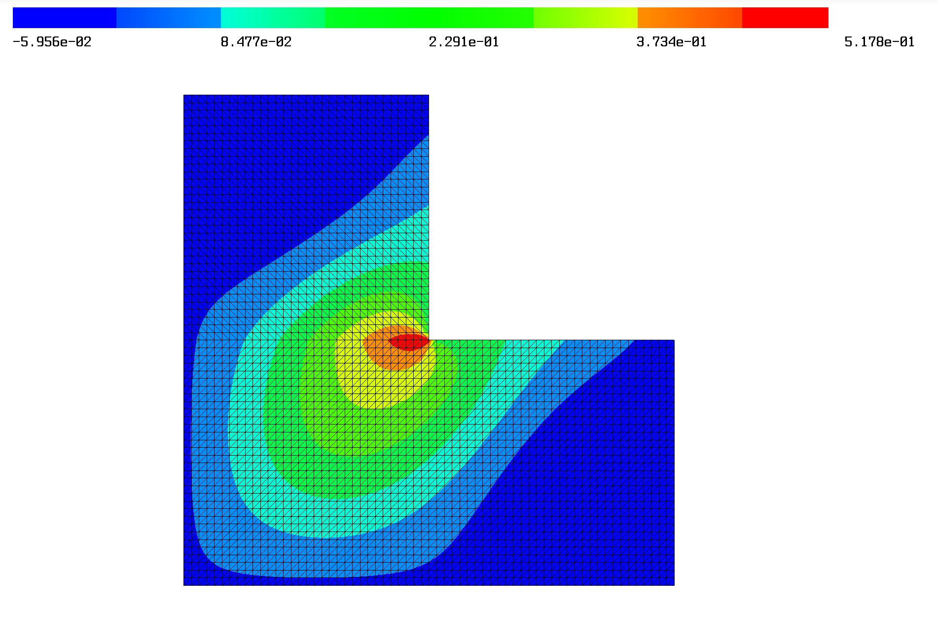
(a) approximation $\overline{v}^{2}$

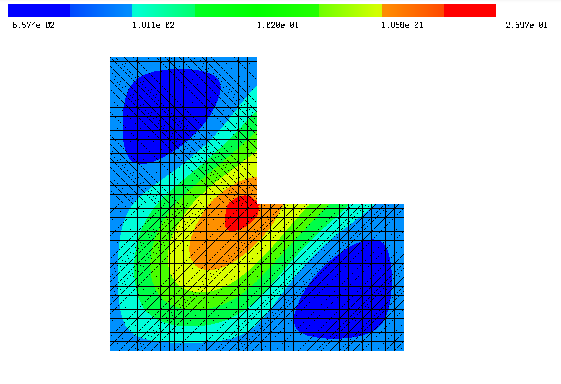
(b) approximation $\overline{v}^{4}$

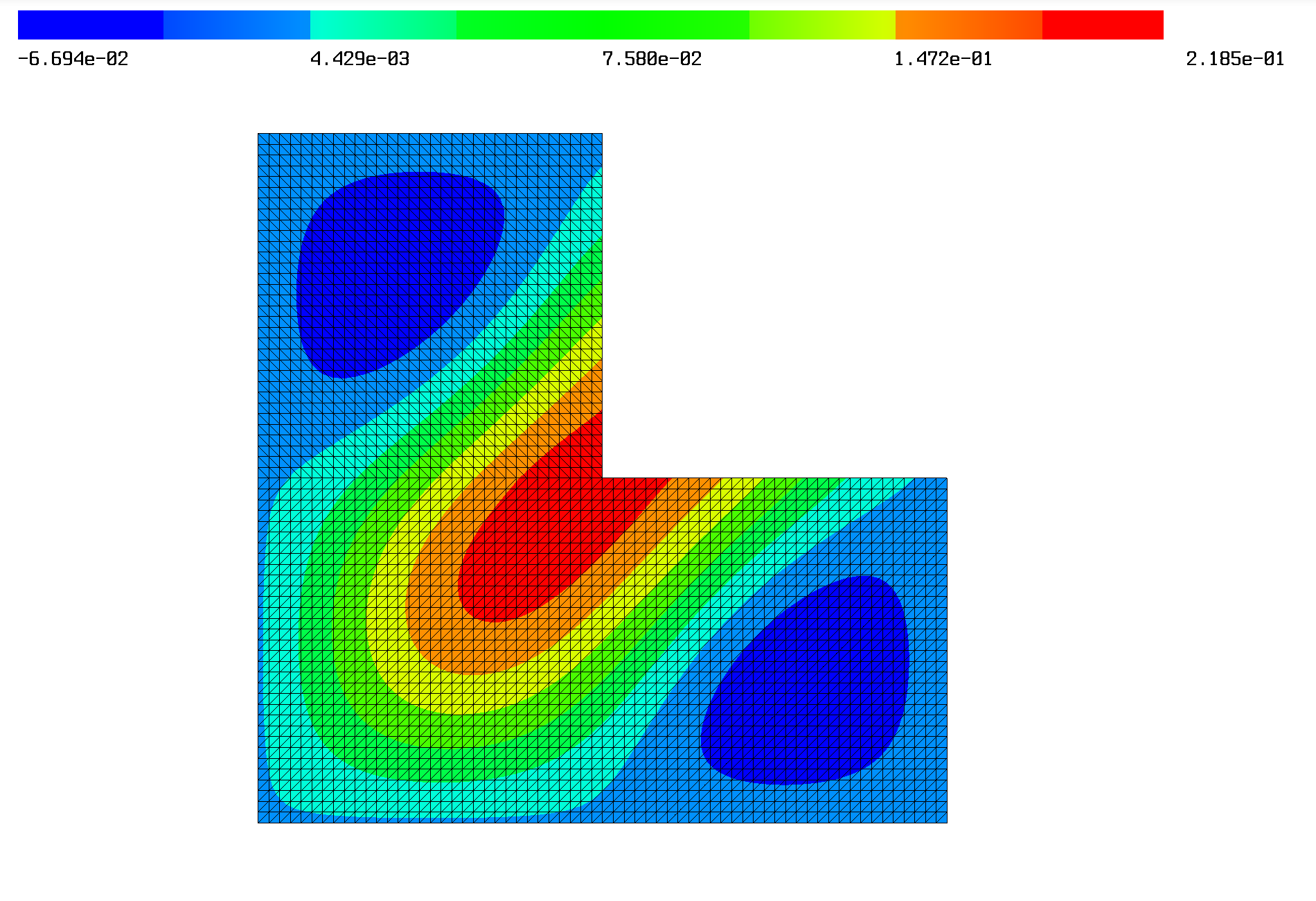
(c) approximation $\overline{v}^{6}$

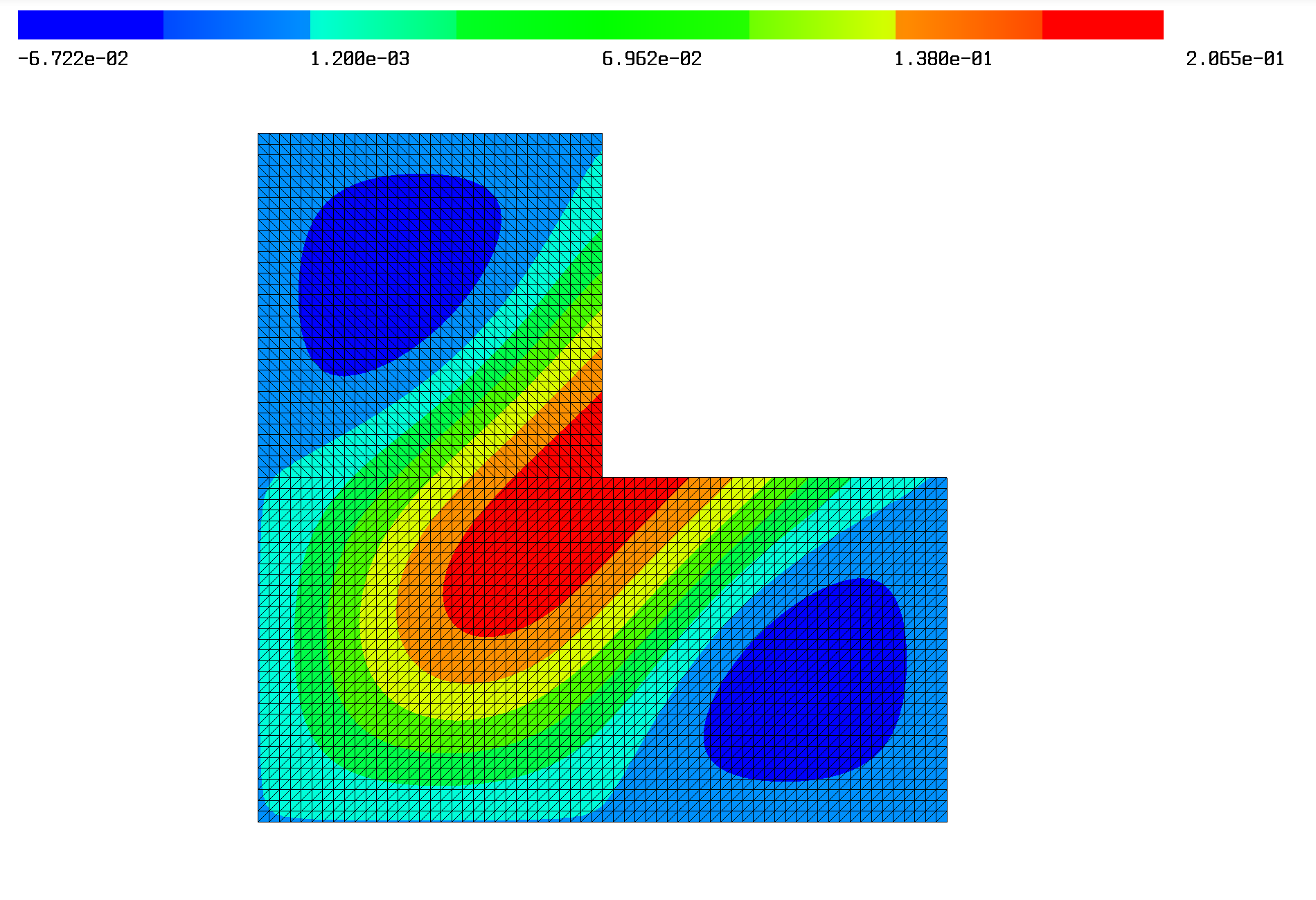
(d) approximation $\overline{v}^{8}$

Figure 4. Global numerical approximation after iterations $2,4,6$ and $8$ of Algorithm 2.1

.

We evaluated the contributions of different parts of the majorant (41), which we denote by $M_{1}^{2}$, $M_{2}^{2}$, and $M_{3}^{2}$, i.e., splitting the majorant according to

$$M_{\oplus}^{2}:=M_{1}^{2}+M_{2}^{2}+M_{3}^{2},$$

where

(54a) $$M_{1}^{2} := \alpha_{1}\displaystyle\sum_{k=1}^{N}\|\bm{y}_{k}-A\nabla v\|^{2}_{A^{-1},{{\omega}}_{k}},$$

(54b) $$M_{2}^{2} := \alpha_{2}\displaystyle\sum_{k=1}^{N}\|{\rm div}\bm{y}_{k}+f\|^{2}_{{{\omega}}_{k}},$$

(54c) $$M_{3}^{2} := \alpha_{3}\displaystyle\sum_{\gamma_{kj}\in\mathcal{E}_{1}}\beta_{kj}^{2}\|(\bm{y}_{k}-\bm{y}_{j})\cdot\bm{n}_{kj}\|_{\gamma_{kj}}^{2}.$$

In the computations we did not perform any optimization of the parameters $\varepsilon_{i}$, $i=1,2,3$, but used $\varepsilon_{1}=\varepsilon_{2}=\varepsilon_{3}=1$ instead. Further used in the computations are the constants $C_{\rm P,\max}=\sqrt{2}/\pi,C_{\min}=1,E_{\max}=2$, $\alpha_{i}$, $i=1,2,3$, as in Remark 3.2, and $\beta_{12}=\beta_{23}=1/\sqrt{\pi{\rm tanh}(\pi)}$.

Tables 1–2 are for different mesh size. The quantities summarized in Table 1 were computed with approximate solutions $v=\overline{v}^{n}$ and a flux corrector $\bm{q}$ on the same mesh with mesh size $h=H$ whereas the results in Table 2 were obtained with a flux corrector on a coarser mesh with mesh size $H>h$.

As we can see, the efficiency index

$$I_{\rm eff}:=\frac{M_{\oplus}(\bm{y},v,f;1,1,1)}{\displaystyle\|\nabla(u-v)\|_{A,\Omega}}$$

in the former case is very good even without optimization of the parameters $\varepsilon_{i}$, $i=1,2,3$, and gets much worse in the latter case. This suggests the strategy to improve a flux corrector that has been computed from a global problem on a coarse mesh with mesh size $H$ by solving local subdomain problems on a fine mesh with mesh size $h$.

Table 1. Contributions to error majorant (41); Evaluation after 16 iterations of Algorithm 2.1; Corrector computed on fine mesh, i.e., $H=h$.

$h$	$M_{1}^{2}$	$M_{2}^{2}$	$M_{3}^{2}$	$M_{\oplus}^{2}$	$I_{\rm eff}$
1/4	8.28e-2	1.49e-1	5.45e-4	2.32e-1	2.96
1/8	2.23e-2	3.80e-2	2.16e-4	6.05e-2	2.96
1/16	5.91e-3	9.56e-3	6.69e-5	1.55e-2	2.98
1/32	1.62e-3	2.39e-3	1.82e-5	4.03e-3	3.04
1/64	4.80e-4	5.98e-4	4.69e-6	1.08e-3	3.15

Table 2. Contributions to error majorant (41); Evaluation after 16 iterations of Algorithm 2.1; Approximations $v=\overline{v}^{n}$ computed on fine mesh with mesh size $h=1/64$, corrector $\bm{q}$ on coarser mesh with mesh size $H>h$.

$H$	$M_{1}^{2}$	$M_{2}^{2}$	$M_{3}^{2}$	$M_{\oplus}^{2}$	$I_{\rm eff}$
1/4	2.75e-3	4.62e-1	1.21e-3	4.66e-1	6.53e1
1/8	1.74e-3	4.06e-1	3.07e-4	4.08e-1	6.11e1
1/16	1.09e-3	3.17e-1	7.61e-5	3.18e-1	5.40e1
1/32	7.17e-4	1.95e-1	1.88e-5	1.96e-1	4.23e1

Next, we tested how the parts $M_{1}^{2}$, $M_{2}^{2}$, and $M_{3}^{2}$ of the majorant $M_{\oplus}^{2}$ change throughout the Schwarz alternating iterative prozess, i.e., for increasing iteration count $n$. The results are presented in Table 3.

Table 3. Contributions to error majorant (41); Increasing number of iterations of Algorithm 2.1; Corrector computed on fine mesh, i.e., $H=h$.

$n$	$M_{1}^{2}$	$M_{2}^{2}$	$M_{3}^{2}$	$M_{\oplus}^{2}$	$I_{\rm eff}$
2	1.26e0	4.27e-2	1.56e-1	1.46e0	1.70
4	5.91e-2	1.99e-3	8.63e-3	6.97e-2	1.72
6	3.57e-3	6.59e-4	4.65e-4	4.70e-3	1.86
8	6.55e-4	6.01e-4	2.57e-5	1.28e-3	2.66

Finally, we tested how the parts $M_{1}^{2}$ and $M_{2}^{2}$, which can be evaluated on different basic subdomains independently from each other, change as the number of iterations $n$ increases. As one can observe, see Table 4, especially $M_{1}$ indicates well which basic subdomains should be processed next by the Schwarz method in order to reduce the global error majorant effectively.

Table 4. Contributions to volume terms of the error majorant (41) from different basic subdomains; Increasing number of iterations of Algorithm 2.1; Corrector computed on fine mesh, i.e., $H=h$.

$n$	$M_{1,\omega_{1}}^{2}$	$M_{1,\omega_{2}}^{2}$	$M_{1,\omega_{3}}^{2}$	$M_{2,\omega_{1}}^{2}$	$M_{2,\omega_{2}}^{2}$	$M_{2,\omega_{3}}^{2}$
2	7.94e-1	3.10e-1	1.60e-1	1.80e-2	2.22e-2	2.50e-3
3	3.59e-2	6.18e-2	1.71e-1	7.60e-4	3.99e-3	3.10e-3
4	3.76e-2	1.31e-2	8.42e-3	8.78e-4	8.89e-4	2.23e-4
7	3.01e-4	3.67e-4	5.54e-4	3.14e-4	1.58e-4	1.39e-4
8	3.03e-4	2.55e-4	9.66e-5	3.15e-4	1.52e-4	1.34e-4

These experiments confirm that the new localized a posteriori error majorant provided by Theorem 3.1 (and estimate (41)) has great potential to become a powerful tool for reliable and cost-efficient iterative solution methods for (elliptic) PDEs by domain decomposition methods.

Future investigations will deal with refining the proposed approach and adapting it to various classes of problems.

Acknowledgements. The first author would like to thank Philip Lederer for his support with the high performance multiphysics finite element software Netgen/NGSolve that served as a platform to conduct the numerical tests.

References

- [1] D. Braess and J. Schöberl. Equilibrated residual error estimator for edge elements. Math. Comp., 77(262):651–672, 2008.
- [2] J.H. Bramble, J.E. Pasciak, J.P. Wang, and J. Xu. Convergence estimates for product iterative methods with applications to domain decomposition. Math. Comp., 57(195):1–21, 1991.
- [3] C.R. Dohrmann. A preconditioner for substructuring based on constrained energy minimization. SIAM J. Sci. Comput., 25(1):246–258, 2003.
- [4] V. Dolean, P. Jolivet, and F. Nataf. An introduction to domain decomposition methods. Society for Industrial and Applied Mathematics (SIAM), Philadelphia, PA, 2015. Algorithms, theory, and parallel implementation.
- [5] Y. Efendiev, J. Galvis, R. Lazarov, and J. Willems. Robust domain decomposition preconditioners for abstract symmetric positive definite bilinear forms. ESAIM: Mathematical Modelling and Numerical Analysis, 46(05):1175–1199, 2012.
- [6] C. Farhat, M. Lesoinne, P. LeTallec, K. Pierson, and D. Rixen. FETI-DP: A dual-primal unified FETI method. I. A faster alternative to the two-level FETI method. Int. J. Numer. Methods Engrg., 50(7):1523–1544, 2001.
- [7] J. Galvis and Y. Efendiev. Domain decomposition preconditioners for multiscale flows in high-contrast media. Multiscale Model. Simul., 8(4):1461–1483, 2010.
- [8] W. Hackbusch. Multi-Grid Methods and Applications. Springer, Berlin Heidelberg, 2003.
- [9] L.V. Kantorovich and V.I. Krylov. Approximate methods of higher analysis. Interscience, 1964.
- [10] D.W. Kelly. The self-equilibration of residuals and complementary a posteriori error estimates in the finite element method. Internat. J. Numer. Methods Engrg., 20(8):1491–1506, 1984.
- [11] J. Kraus. Algebraic multilevel preconditioning of finite element matrices using local Schur complements. Numer. Linear Algebra Appl., 13:49–70, 2006.
- [12] J. Kraus. Additive Schur complement approximation and application to multilevel preconditioning. SIAM J. Sci. Comput., 34:A2872–A2895, 2012.
- [13] J. Kraus, M. Lymbery, and S. Margenov. Auxiliary space multigrid method based on additive Schur complement approximation. Numer. Linear Algebra Appl., 22(6):965–986, 2015.
- [14] J. Kraus, R. Lazarov, M. Lymbery, S. Margenov, and L. Zikatanov. Preconditioning heterogeneous problems by additive Schur complement approximation and applications. SIAM J. Sci. Comput., 38(2):A875–A898, 2016.
- [15] Y. Kuznetsov. Algebraic multigrid domain decomposition methods. Sov. J. Numer. Anal. Math. Modelling., 4(5):351–379, 1989.
- [16] P. Ladevèze and D. Leguillon. Error estimate procedure in the finite element method and applications. SIAM J. Numer. Anal., 20(3):485–509, 1983.
- [17] P.-L. Lions. Interprétation stochastique de la méthode alternée de Schwarz. C. R. Acad. Sci. Paris, 268:325–328, 1978.
- [18] P.-L. Lions. On the Schwarz alternating method. I. In R. Glowinski, G. H. Golub, G. A. Meurant, and J. Périaux, editors, First International Symposium on Domain Decomposition Methods for Partial Differential Equations, pages 1–42, Paris, France, 1987. SIAM, Philadelphia, PA.
- [19] P.-L. Lions. On the Schwarz alternating method. II. In T. Chan, R. Glowinski, J. Périaux, and O. Widlund, editors, Second International Symposium on Domain Decomposition Methods for Partial Differential Equations, pages 47–70, Paris, France, 1989. SIAM, Los Angeles, CA.
- [20] O. Mali, P. Neittaanmäki, and S. Repin. Accuracy verification methods, volume 32 of Computational Methods in Applied Sciences. Springer, Dordrecht, 2014. Theory and algorithms.
- [21] J. Mandel. Balancing domain decomposition. Comm. Numer. Methods Engrg., 9(3):233–241, 1993.
- [22] J. Mandel and C.R. Dohrmann. Convergence of a balancing domain decomposition by constraints and energy minimization. Numer. Linear Algebra Appl., 10(7):639–659, 2003.
- [23] J. Mandel, C.R. Dohrmann, and R. Tezaur. An algebraic theory for primal and dual substructuring methods by constraints. Appl. Numer. Math., 54(2):167–193, 2005.
- [24] J. Mandel and B. Sousedík. Adaptive selection of face coarse degrees of freedom in the BDDC and FETI-DP iterative substructuring methods. Comput. Methods Appl. Mech. Engrg., 196(8):1389–1399, 2007.
- [25] T.P.A. Mathew. Domain Decomposition Methods for the Numerical Solution of Partial Differential Equations. Springer, Berlin Heidelberg, 2008.
- [26] A.M. Matsokin and S.V. Nepomnyashchikh. Convergence of the Schwarz alternation method over subdomains without overlap. In Approximation and interpolation methods (Novosibirsk, 1980), pages 85–97. Akad. Nauk SSSR Sibirsk. Otdel., Vychisl. Tsentr, Novosibirsk, 1981. Translated in Soviet J. Numer. Anal. Math. Modelling 4 (1989), no. 6, 479–485.
- [27] A.M. Matsokin and S.V. Nepomnyashchikh. The Schwarz alternation method in a subspace. Izv. Vyssh. Uchebn. Zaved. Mat., (10):61–66, 85, 1985.
- [28] S.G. Mikhlin. On the Schwarz algorithm. Doklady Akad. Nauk SSSR (N.S.), 77:569–571, 1951.
- [29] S.G. Mikhlin. Variational methods in mathematical physics. A Pergamon Press Book. The Macmillan Co., New York, 1964. Translated by T. Boddington; editorial introduction by L. I. G. Chambers.
- [30] A.I Nazarov and S. Repin. Exact constants in Poincaré type inequalities for functions with zero mean boundary traces. Math Methods Appl Sci., 38:3195–3207, 2015.
- [31] O. Nevanlinna. Remarks on Picard-Lindelöf iteration. II. BIT, 29(3):535–562, 1989.
- [32] A. Ostrowski. Les estimations des erreurs a posteriori dans les procédés itératifs. C. R. Acad. Sci. Paris Sér. A-B, 275:A275–A278, 1972.
- [33] S. Repin. A posteriori error estimation methods for partial differential equations. In Lectures on advanced computational methods in mechanics, volume 1 of Radon Ser. Comput. Appl. Math., pages 161–226. Walter de Gruyter, Berlin, 2007.
- [34] S.I. Repin. A posteriori error estimation for variational problems with uniformly convex functionals. Math. Comp., 69(230):481–500, 2000.
- [35] M.V. Sarkis Martins. Schwarz preconditioners for elliptic problems with discontinuous coefficients using conforming and non-conforming elements. ProQuest LLC, Ann Arbor, MI, 1994. Thesis (Ph.D.)–New York University.
- [36] R. Scheichl, P. Vassilevski, and L. Zikatanov. Weak approximation properties of elliptic projections with functional constraints. Multiscale Model. Simul., 9(4):1677–1699, 2011.
- [37] H.A. Schwarz. Ueber einige Abbildungsaufgaben. J. Reine Angew. Math., 70:105–120, 1869.
- [38] D.R. Stoutemyer. Numerical implementation of the Schwarz alternating procedure for elliptic partial differential equations. SIAM J. Numer. Anal., 10:308–326, 1973.
- [39] J.L. Synge. The hypercircle method. In Studies in numerical analysis (papers in honour of Cornelius Lanczos on the occasion of his 80th birthday), pages 201–217. 1974.
- [40] A. Toselli and O. Widlund. Domain Decomposition Methods - Algorithms and Theory. Springer, Berlin Heidelberg, Germany, 2005.
- [41] U. Trottenberg, C.W. Oosterlee, and A. Schüller. Multigrid. Academic Press Inc., San Diego, CA, 2001.
- [42] P. Vassilevski. Multilevel Block Factorization Preconditioners: Matrix-based Analysis and Algorithms for Solving Finite Element Equations. Springer, New York, 2008.
- [43] R. Verfürth. A review of a posteriori error estimation and adaptive mesh-refinement techniques. John Wiley and Sons Ltd, 1996.
- [44] J. Xu. The auxiliary space method and optimal multigrid preconditioning techniques for unstructured grids. Computing, 56:215–235, 1996.
- [45] J. Xu and L. Zikatanov. The method of alternating projections and the method of subspace corrections in Hilbert space. J. Amer. Math. Soc., 15(3):573–597, 2002.