One-loop contributions to the decay $H\rightarrow\nu_{l}\bar{\nu}_{l}\gamma$ in standard model revisited

Abstract

One-loop contributions to the decay $H\rightarrow\nu_{l}\bar{\nu}_{l}\gamma$ with $l=e,\mu,\tau$ within standard model framework are revisited in this paper. We derive two representations for the form factors in this calculation. As a result, the computations are not only checked numerically by verifying the ultraviolet finiteness of the results but also confirming the ward identity of the amplitude. We find that the results are good stability with varying ultraviolet cutoff parameters as well as satisfy the ward identity. In phenomenological results, all the physical results are examined with the present input parameters. Especially, we study the partial decay widths for the decay channels in both cases of the detected photon and invisible photon. Differential decay widths are also generated as a function of energy of final photon.

1 Introduction

Today one of the main purposes of experimental program at the High Luminosity Large Hadron Collider (HL-LHC) [1, 2] and Future Lepton Colliders [3] is to measure precisely the properties of standard model-like (SM-like) Higgs boson. In this program, searching for all decay modes of Higgs boson are priority tasks and have to be probed as precisely as possible. Because the partial decay widths of Higgs boson provide an important information for answering the nature of Higgs sector (for our deeper understanding of the dynamics of electroweak symmetry breaking). In all decay channels of Higgs boson, $H\rightarrow$ invisible particles and $H\rightarrow\gamma$ plus invisible particles [4, 5, 6, 7, 8, 9, 10] are also great of interest by following aspects: (i) these processes can be probed at future colliders [4, 5, 6, 8, 10] for testing the standard model (SM) at modern energy regions; (ii) many new heavy particles such as new extra gauge bosons, charged (and neutral) scalar particles may exchange in the loop diagrams of the aforementioned decay channels. Thus, the decay processes could provide a useful tool for testing the SM and investigating possible new physics.

We know that the precise evaluations for the standard model background play a crucial role in searching for new physics. It means that the theoretical calculations for one-loop contributing to $H\rightarrow\nu_{l}\bar{\nu}_{l}\gamma$ are necessary. In Ref. [11], one-loop formulas for $H\rightarrow\nu_{l}\bar{\nu}_{l}\gamma$ within SM framework have provided. In view of the importance of the decay channels we revisit the calculation for the decay processes with extending the previous computation and updating numerical predictions using the present values of input parameters. The analytic results for one-loop form factors are expressed in terms of Passarino-Veltman functions (called as PV-functions) which they can be evaluated numerically by using package LoopTools [14]. In comparison with the previous work, the evaluations in the present paper are extended by following points. Firstly, two representations for the form factors are derived in this calculation. As a result, the computations are not only checked numerically by verifying the ultraviolet finiteness of the results but also confirming the ward identity of the amplitude. We find that the results are good stability with varying ultraviolet cutoff parameters as well as follow the ward identity of the amplitude. Secondly, we study the partial decay widths for the decay channels in both cases of the detected photon and invisible photon using the present values of input parameters. Lastly, all the PV-functions are also reduced to scalar one-, two-, three- and four-point functions in this paper. In further, we point out that one uses the generalised hypergeometric functions in [15, 17, 16] at general space-time dimensions $d$ for scalar one-loop integrals, the form factors will be valid in general $d$. Therefore, the form factors can be performed at higher-power $\varepsilon$-expansion which may be taken into account in two-loop and higher-loop contributing to these channels.

The layout of the paper is as follows: In section 2, detailed calculations for one-loop contributions to $H\rightarrow\nu_{l}\bar{\nu}_{l}\gamma$ are presented. Numerical test for the computations and physical results for the decay processes are also shown in this sections. Conclusions and outlook are devoted in section $3$. In appendices, reduction formulas for scalar PV-functions are presented.

2 Calculation

Detailed calculations for one-loop contributions to $H\rightarrow\nu_{l}\bar{\nu}_{l}\gamma$ are presented in this section. Two different representations for one-loop form factors are derived. Numerical tests for the computation and physical results for the decay processes are then shown in the next subsections.

2.1 Analytic results

We devote detailed the calculation for the decay channels $H(p)\rightarrow\nu_{l}(q_{1})\bar{\nu}_{l}(q_{2})\gamma(q_{3})$ in this subsection. Within the standard model framework the decay processes consist of $W$ bosons and fermions exchanging in one-loop triangle diagrams (seen Fig. 1 and Fig. 2 respectively) as well as $6$ one-loop box diagrams (shown in Fig. 3) in unitary gauge.

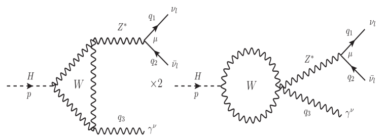
Figure 1: $W$-bosons exchanging in the one-loop triangle diagrams of $H\rightarrow\nu_{l}\bar{\nu_{l}}\gamma$ in unitary gauge.

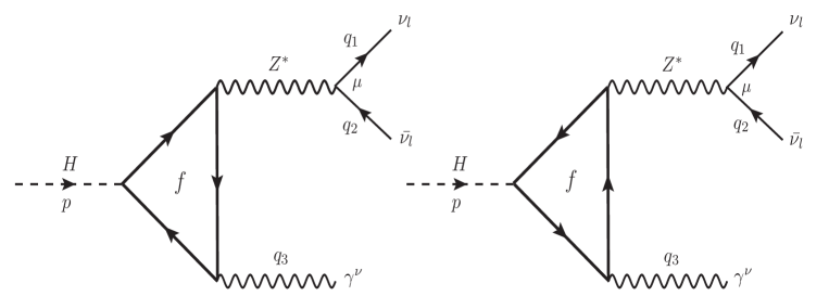
Figure 2: Fermion $f$ exchanging in the one-loop triangle diagrams of $H\rightarrow\nu_{l}\bar{\nu_{l}}\gamma$ in unitary gauge.

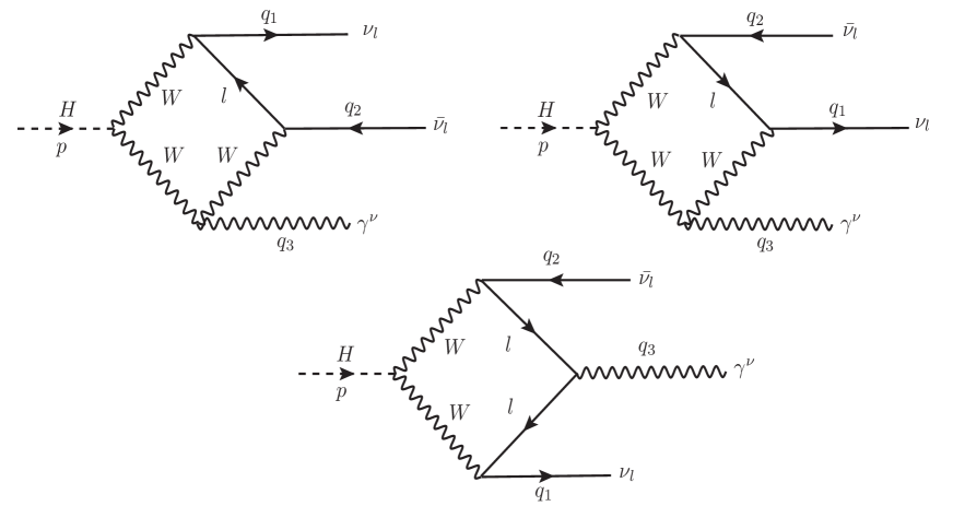
Figure 3: $W$-boson and lepton $l$ particles exchanging in the one-loop box diagrams of $H\rightarrow\nu_{l}\bar{\nu_{l}}\gamma$ in unitary gauge.

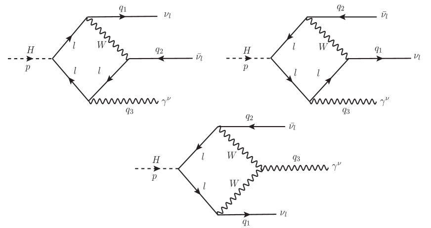
Figure 4: Lepton $l$ and $W$-boson particles exchanging in the one-loop box diagrams of $H\rightarrow\nu_{l}\bar{\nu_{l}}\gamma$ in unitary gauge.

In general, one-loop amplitude of the decay channels can be divided as follows:

$$\mathcal{A}=\mathcal{A}^{(W)}_{\text{tri}}+\mathcal{A}^{(f)}_{\text{tri}}+\mathcal{A}^{(W)}_{\text{box}}+\mathcal{A}^{(l)}_{\text{box}}.$$ (1)

In this formula, $\mathcal{A}^{(W)}_{\text{tri}}$ presents for the contributions of one-loop triangle Feynman diagrams with $W$ boson internal lines (shown in Fig. 1). The term $\mathcal{A}^{(f)}_{\text{tri}}$ is for the amplitude of one-loop triangle Feynman diagrams with exchanging fermions in the loop (seen in Fig. 2). In the same notations, $\mathcal{A}^{(W)}_{\text{box}}(\mathcal{A}^{(l)}_{\text{box}})$ is corresponding to the amplitude of one-loop box diagrams in Fig. 3 (and in Fig. 4 respectively).

For on-shell external photon, the ward identity is implied. As a result, we have the following relation: $q_{3}^{\nu}\epsilon_{\nu}^{*}=0$ where $q_{3}^{\nu}$, $\epsilon_{\nu}^{*}$ are corresponding to momentum and polarization vector of photon. Kinematic invariant variables involving to this decay process are concerned:

$$p^{2} = M_{H}^{2},\;q_{1}^{2}=q_{2}^{2}=q_{3}^{2}=0,\;q_{12}=(q_{1}+q_{2})^{2}=2q_{1}\cdot q_{2},\;q_{13}=2q_{1}\cdot q_{3},\;q_{23}=2q_{2}\cdot q_{3}.$$ (2)

With this definition, one confirms that $q_{12}+q_{13}+q_{23}=M_{H}^{2}$.

We first write down all Feynman amplitudes for the above diagrams. With the help of Package-X [13], all Dirac traces and Lorentz contractions in $d$ dimensions are handled. Subsequently, the amplitudes are then expressed in terms of tensor one-loop integrals. By following tensor reduction for one-loop integrals in [12], all tensor one-loop integrals are written in terms of PV-functions (scalar $PV$-coefficient functions are labled as $A_{ijk\cdots},B_{ijk\cdots},C_{ijk\cdots}$ and $D_{ijk\cdots}$ for $i,j,k\cdots=1,2,3$ as in Ref. [12]). In this paper, we also reduce the PV-functions to scalar one-loop integrals (labeled as $A_{0},B_{0},C_{0}$ and $D_{0}$ [12]). Latter, these scalar functions $A_{0},B_{0},C_{0}$ and $D_{0}$ can be evaluated numerically by using LoopTools. Furthermore, one can use hypergeometric representations in [15, 17, 16] for these scalar functions in general $d$.

2.1.1 First expressions for form factors

We first arrive at one-loop three-point Feynman diagrams with $W$ boson internal lines (as shown in Fig. 1). The corresponding amplitude for the above Feynman diagrams is decomposed into Lorentz invariant structure as follows:

$$\mathcal{A}^{(W)}_{\text{tri}} = \Big{[}F_{1}^{(W)}q_{3}^{\mu}q^{\nu}+F_{2}^{(W)}g^{\mu\nu}\Big{]}\bar{u}(q_{1})\gamma^{\mu}\;P_{L}v(q_{2})\epsilon^{*}_{\nu}(q_{3}).$$ (3)

Where we have used $P_{L}=\dfrac{1-\gamma_{5}}{2}$. Applying the tensor reduction method in [12], all form factors in this formula are computed. Analytic results for the form factors are expressed in terms of $B_{0}$ and $C_{0}$ functions as follows:

$$F_{1}^{(W)} = \dfrac{\alpha^{2}}{2M_{W}^{3}s_{W}^{3}(d-2)(M_{H}^{2}-q_{12})^{2}}\dfrac{1}{q_{12}-M_{Z}^{2}+i\Gamma_{Z}M_{Z}}\times$$

$$\times\Bigg{\{}\Big{[}M_{H}^{2}(2M_{W}^{2}-q_{12})+4M_{W}^{4}(d-1)-2M_{W}^{2}q_{12}\Big{]}\times$$

$$\times\Big{[}\Big{(}M_{H}^{2}(d-4)+(2-d)q_{12}\Big{)}B_{0}(M_{H}^{2},M_{W}^{2},M_{W}^{2})+2q_{12}B_{0}(q_{12},M_{W}^{2},M_{W}^{2})\Big{]}$$

$$+4M_{W}^{2}(M_{H}^{2}-q_{12})\Big{[}2M_{W}^{2}(M_{H}^{2}-q_{12})(2d-5)-4M_{W}^{4}(d-1)$$

$$\hskip 71.13188pt+q_{12}^{2}(d-2)-M_{H}^{2}q_{12}(d-3)\Big{]}C_{0}(0,q_{12},M_{H}^{2},M_{W}^{2},M_{W}^{2},M_{W}^{2})\Bigg{\}}.$$

Here $s_{W}=\sin\theta_{W}$, $\theta_{W}$ is weak mixing angle and $d=4-2\varepsilon$ is space-time dimension. In this paper, we also compute the form factor $F_{2}^{(W)}$ which its analytical result is shown in the next subsection. In general, $F_{2}^{(W)}$ may take different form with $F_{1}^{(W)}$. Following the ward identity, one confirms that

$$F_{2}^{(W)}=\dfrac{q_{12}-M_{H}^{2}}{2}F_{1}^{(W)}$$ (5)

It can be observed the relation in Eq. (5) analytically by performing $\varepsilon$-expansion for the form factors. Both the expressions for $F_{1}^{(W)}$ and $F_{2}^{(W)}$ give same result (seen appendix $B$). We also note that the relation can be also verified numerically in next subsections.

We now consider Feynman amplitude for one-loop triangle diagrams with fermion internal lines. Following the same procedure, the amplitude is casted into the form of

$$\mathcal{A}^{(f)}_{\text{tri}} = \Big{[}F_{1}^{(f)}q_{3}^{\mu}q^{\nu}+F_{2}^{(f)}g^{\mu\nu}\Big{]}\bar{u}(q_{1})\gamma^{\mu}P_{L}v(q_{2})\epsilon^{*}_{\nu}(q_{3}).$$ (6)

All form factors in this equation are evaluated by using the tensor reduction method in [12]. The results read:

$$F_{1}^{(f)} = \dfrac{\alpha^{2}N_{C}^{f}Q_{f}m_{f}^{2}\Big{(}T_{3}^{f}-2Q_{f}s_{W}^{2}\Big{)}}{M_{W}c_{W}^{2}s_{W}^{3}(d-2)(M_{H}^{2}-q_{12})^{2}}\dfrac{1}{q_{12}-M_{Z}^{2}+i\Gamma_{Z}M_{Z}}\times$$

$$\times\Bigg{\{}\Big{[}2M_{H}^{2}(d-4)-2q_{12}(d-2)\Big{]}B_{0}(M_{H}^{2},m_{f}^{2},m_{f}^{2})+4q_{12}B_{0}(q_{12},m_{f}^{2},m_{f}^{2})$$

$$+\Big{[}(d-2)(M_{H}^{2}-q_{12})^{2}-8m_{f}^{2}(M_{H}^{2}-q_{12})\Big{]}C_{0}(0,q_{12},M_{H}^{2},m_{f}^{2},m_{f}^{2},m_{f}^{2})\Bigg{\}}.$$

Here $N_{C}^{f}\;(Q_{f})$ is number of color and charge quantum number of fermion $f$. While $T_{3f}$ is hypercharge of fermion $f$. The form factor $F_{2}^{(f)}$ is shown in next subsection. It is important to note that all fermions with non-zero masses in the loop are considered in present paper.

We turn our attention to one-loop four-point Feynman diagrams contributing to these decay processes. We have one-loop box diagrams that Higgs couple directly to $W$ bosons (as shown in Fig. 3). The corresponding amplitude is expressed in Lorentz invariant structure as follows:

$$\mathcal{A}^{(W)}_{\text{box}} = \bar{u}(q_{1})\Big{\{}F_{3}^{(W)}q_{1}^{\nu}\not{q_{3}}+F_{4}^{(W)}q_{2}^{\nu}\not{q_{3}}+F_{5}^{(W)}\gamma^{\nu}\Big{\}}P_{L}v(q_{2})\epsilon^{*}_{\nu}(q_{3}).$$ (8)

Where $F_{5}^{(W)}=-F_{3}^{(W)}(q_{1}\cdot q_{3})-F_{4}^{(W)}(q_{2}\cdot q_{3})$. Analytic results for all form factors are shown in terms of PV-functions as follows:

$$F_{3}^{(W)} = \dfrac{\alpha^{2}}{2M_{W}^{5}s_{W}^{3}}\times$$ (9)

$$\times\Big{\{}(M_{H}^{2}M_{W}^{2}+2M_{W}^{4})\Big{[}(C_{22}+C_{12}+C_{2})(0,q_{12},M_{H}^{2},M_{W}^{2},M_{W}^{2},M_{W}^{2})$$

$$\hskip 106.69783pt+(C_{22}+C_{12}+C_{2})(q_{12},0,M_{H}^{2},M_{W}^{2},M_{W}^{2},M_{W}^{2})\Big{]}$$

$$\hskip 7.11317pt-M_{W}^{2}m_{l}^{2}\Big{[}(C_{22}+C_{12}+C_{2})(0,0,q_{13},m_{l}^{2},m_{l}^{2},M_{W}^{2})$$

$$\hskip 56.9055pt+(C_{22}+C_{12}+C_{2})(0,0,q_{13},m_{l}^{2},M_{W}^{2},M_{W}^{2})\Big{]}$$

$$\hskip 7.11317pt+2M_{W}^{4}m_{l}^{2}\Big{[}D_{0}(0,0,0,M_{H}^{2};q_{12},q_{13};M_{W}^{2},m_{l}^{2},M_{W}^{2},M_{W}^{2})$$

$$\hskip 56.9055pt+D_{0}(0,0,0,M_{H}^{2};q_{23},q_{12};M_{W}^{2},M_{W}^{2},m_{l}^{2},M_{W}^{2})$$

$$\hskip 56.9055pt+D_{0}(0,0,0,M_{H}^{2};q_{23},q_{13};M_{W}^{2},m_{l}^{2},m_{l}^{2},M_{W}^{2})\Big{]}$$

$$\hskip 7.11317pt+\Big{[}M_{W}^{2}m_{l}^{2}(M_{H}^{2}+2M_{W}^{2})+2(d-2)M_{W}^{6}\Big{]}\times$$

$$\hskip 7.11317pt\times\Big{[}(D_{33}+D_{23})(0,0,0,M_{H}^{2};q_{12},q_{13};M_{W}^{2},m_{l}^{2},M_{W}^{2},M_{W}^{2})$$

$$\hskip 56.9055pt+(D_{33}+D_{23})(0,0,0,M_{H}^{2};q_{23},q_{13};M_{W}^{2},m_{l}^{2},m_{l}^{2},M_{W}^{2})$$

$$\hskip 56.9055pt+(D_{33}+D_{23}+D_{13})(0,0,0,M_{H}^{2};q_{23},q_{12};M_{W}^{2},M_{W}^{2},m_{l}^{2},M_{W}^{2})\Big{]}$$

$$\hskip 7.11317pt+\Big{[}M_{W}^{2}m_{l}^{2}(M_{H}^{2}+2M_{W}^{2})+2(d-4)M_{W}^{6}\Big{]}\times$$

$$\hskip 7.11317pt\times\Big{[}D_{3}(0,0,0,M_{H}^{2};q_{12},q_{13};M_{W}^{2},m_{l}^{2},M_{W}^{2},M_{W}^{2})$$

$$\hskip 56.9055pt+D_{3}(0,0,0,M_{H}^{2};q_{23},q_{12};M_{W}^{2},M_{W}^{2},m_{l}^{2},M_{W}^{2})$$

$$\hskip 56.9055pt+D_{3}(0,0,0,M_{H}^{2};q_{23},q_{13};M_{W}^{2},m_{l}^{2},m_{l}^{2},M_{W}^{2})\Big{]}$$

$$\hskip 7.11317pt+4M_{W}^{4}\Big{[}C_{0}(0,q_{12},M_{H}^{2},M_{W}^{2},M_{W}^{2},M_{W}^{2})$$

$$\hskip 56.9055pt-M_{W}^{2}D_{2}(0,0,0,M_{H}^{2};q_{12},q_{13};M_{W}^{2},m_{l}^{2},M_{W}^{2},M_{W}^{2})\Big{]}\Big{\}}.$$

Analytic formula for another form factor is shown

$$F_{4}^{(W)} = \dfrac{\alpha^{2}}{2M_{W}^{5}s_{W}^{3}}\times$$

$$\times\Big{\{}(M_{H}^{2}M_{W}^{2}+2M_{W}^{4})\Big{[}(C_{22}+C_{12}+C_{2})(0,q_{12},M_{H}^{2},M_{W}^{2},M_{W}^{2},M_{W}^{2})$$

$$\hskip 113.81102pt+(C_{22}+C_{12}+C_{2})(q_{12},0,M_{H}^{2},M_{W}^{2},M_{W}^{2},M_{W}^{2})\Big{]}$$

$$\hskip 7.11317pt-M_{W}^{2}m_{l}^{2}\Big{[}(C_{22}+C_{12}+C_{2})(0,0,q_{23},M_{W}^{2},m_{l}^{2},m_{l}^{2})$$

$$\hskip 56.9055pt+(C_{22}+C_{12}+C_{2})(0,0,q_{23},M_{W}^{2},M_{W}^{2},m_{l}^{2})\Big{]}$$

$$\hskip 7.11317pt+2M_{W}^{4}m_{l}^{2}\Big{[}D_{0}(0,0,0,M_{H}^{2};q_{12},q_{13};M_{W}^{2},m_{l}^{2},M_{W}^{2},M_{W}^{2})$$

$$\hskip 56.9055pt+D_{0}(0,0,0,M_{H}^{2};q_{23},q_{12};M_{W}^{2},M_{W}^{2},m_{l}^{2},M_{W}^{2})$$

$$\hskip 56.9055pt+D_{0}(0,0,0,M_{H}^{2};q_{23},q_{13};M_{W}^{2},m_{l}^{2},m_{l}^{2},M_{W}^{2})\Big{]}$$

$$\hskip 7.11317pt+\Big{[}2M_{W}^{2}m_{l}^{2}(M_{H}^{2}+2M_{W}^{2})+4(d-2)M_{W}^{6}\Big{]}\times$$

$$\hskip 7.11317pt\times\Big{[}D_{23}(0,0,0,M_{H}^{2};q_{23},q_{12};M_{W}^{2},M_{W}^{2},m_{l}^{2},M_{W}^{2})$$

$$\hskip 56.9055pt+D_{23}(0,0,0,M_{H}^{2};q_{23},q_{13};M_{W}^{2},m_{l}^{2},m_{l}^{2},M_{W}^{2})\Big{]}$$

$$\hskip 7.11317pt+\Big{[}M_{W}^{2}m_{l}^{2}(M_{H}^{2}+2M_{W}^{2})+2(d-2)M_{W}^{6}\Big{]}\times$$

$$\hskip 7.11317pt\times\Big{[}(D_{33}+D_{23}+D_{13})(0,0,0,M_{H}^{2};q_{12},q_{13};M_{W}^{2},m_{l}^{2},M_{W}^{2},M_{W}^{2})$$

$$\hskip 28.45274pt+(D_{33}+D_{22}+D_{13}+D_{12})(0,0,0,M_{H}^{2};q_{23},q_{12};M_{W}^{2},M_{W}^{2},m_{l}^{2},M_{W}^{2})$$

$$\hskip 28.45274pt+(D_{33}+D_{22}+D_{13}+D_{12})(0,0,0,M_{H}^{2};q_{23},q_{13};M_{W}^{2},m_{l}^{2},m_{l}^{2},M_{W}^{2})\Big{]}$$

$$\hskip 7.11317pt+\Big{[}M_{W}^{2}m_{l}^{2}(M_{H}^{2}+2M_{W}^{2})+2dM_{W}^{6}\Big{]}\times$$

$$\hskip 7.11317pt\times\Big{[}D_{3}(0,0,0,M_{H}^{2};q_{12},q_{13};M_{W}^{2},m_{l}^{2},M_{W}^{2},M_{W}^{2})$$

$$\hskip 56.9055pt+(D_{3}+D_{2})(0,0,0,M_{H}^{2};q_{23},q_{12};M_{W}^{2},M_{W}^{2},m_{l}^{2},M_{W}^{2})$$

$$\hskip 56.9055pt+(D_{3}+D_{2})(0,0,0,M_{H}^{2};q_{23},q_{13};M_{W}^{2},m_{l}^{2},m_{l}^{2},M_{W}^{2})\Big{]}$$

$$\hskip 7.11317pt+4M_{W}^{6}\Big{[}D_{0}(0,0,0,M_{H}^{2};q_{23},q_{12};M_{W}^{2},M_{W}^{2},m_{l}^{2},M_{W}^{2})$$

$$\hskip 56.9055pt+(D_{0}+D_{1})(0,0,0,M_{H}^{2};q_{23},q_{13};M_{W}^{2},m_{l}^{2},m_{l}^{2},M_{W}^{2})$$

$$\hskip 56.9055pt+(D_{2}+D_{1}+D_{0})(0,0,0,M_{H}^{2};q_{12},q_{13};M_{W}^{2},m_{l}^{2},M_{W}^{2},M_{W}^{2})\Big{]}$$

$$\hskip 7.11317pt+4M_{W}^{4}C_{0}(0,q_{12},M_{H}^{2};M_{W}^{2},M_{W}^{2},M_{W}^{2})\Big{\}}.$$

We have different kinds of $D$-coefficient functions relating to tensor reduction for box diagrams appear in all the above form factors. In principle, tensor one-loop box integrals with rank $P=4$ appear in the amplitude of each diagram. However, these tensor integrals are cancelled out. As a results, we have up to $D_{ij}$ (for $i,j=1,\cdots 3$) functions contributing to the aforementioned form factors.

We finally consider all one-loop box diagrams in Fig. 4 in which Higgs couples directly to leptons. Amplitude for the diagrams are given as the same form in Eq. (8):

$$\mathcal{A}^{(l)}_{\text{box}} = \bar{u}(q_{1})\Big{\{}F_{3}^{(l)}q_{1}^{\nu}\not{q_{3}}+F_{4}^{(l)}q_{2}^{\nu}\not{q_{3}}+F_{5}^{(l)}\gamma^{\nu}\Big{\}}P_{L}v(q_{2})\epsilon^{*}_{\nu}(q_{3})$$ (11)

with $F_{5}^{(l)}=-F_{3}^{(l)}(q_{1}\cdot q_{3})-F_{4}^{(l)}(q_{2}\cdot q_{3})$. All related form factors read as follows:

$$F_{3}^{(l)} = \dfrac{\alpha^{2}}{2M_{W}^{3}s_{W}^{3}}m_{l}^{2}\times$$ (12)

$$\times\Big{\{}(C_{22}+C_{12}+C_{2})(0,0,q_{13},M_{W}^{2},m_{l}^{2},m_{l}^{2})+(C_{22}+C_{12}+C_{2})(0,0,q_{13},M_{W}^{2},M_{W}^{2},m_{l}^{2})$$

$$\hskip 7.11317pt+\Big{[}(6-d)M_{W}^{2}-m_{l}^{2}\Big{]}D_{2}(0,0,0,M_{H}^{2};q_{12},q_{13};m_{l}^{2},M_{W}^{2},m_{l}^{2},m_{l}^{2})$$

$$\hskip 7.11317pt+\Big{[}2m_{l}^{2}+2(d-2)M_{W}^{2}\Big{]}\Big{[}(D_{33}+D_{23})(0,0,0,M_{H}^{2};q_{12},q_{13};m_{l}^{2},M_{W}^{2},m_{l}^{2},m_{l}^{2})$$

$$\hskip 113.81102pt+(D_{33}+D_{23})(0,0,0,M_{H}^{2};q_{23},q_{13};m_{l}^{2},M_{W}^{2},M_{W}^{2},m_{l}^{2})$$

$$\hskip 113.81102pt+(D_{33}+D_{23}+D_{13})(0,0,0,M_{H}^{2};q_{23},q_{12};m_{l}^{2},m_{l}^{2},M_{W}^{2},m_{l}^{2})\Big{]}$$

$$\hskip 7.11317pt+\Big{[}(d+2)M_{W}^{2}+m_{l}^{2}\Big{]}\Big{[}D_{3}(0,0,0,M_{H}^{2};q_{12},q_{13};m_{l}^{2},M_{W}^{2},m_{l}^{2},m_{l}^{2})$$

$$\hskip 113.81102pt+D_{3}(0,0,0,M_{H}^{2};q_{23},q_{12};m_{l}^{2},m_{l}^{2},M_{W}^{2},m_{l}^{2})$$

$$\hskip 113.81102pt+D_{3}(0,0,0,M_{H}^{2};q_{23},q_{13};m_{l}^{2},M_{W}^{2},M_{W}^{2},m_{l}^{2})\Big{]}$$

$$\hskip 7.11317pt+2M_{W}^{2}\Big{[}D_{0}(0,0,0,M_{H}^{2};q_{12},q_{13};m_{l}^{2},M_{W}^{2},m_{l}^{2},m_{l}^{2})$$

$$\hskip 113.81102pt+D_{0}(0,0,0,M_{H}^{2};q_{23},q_{12};m_{l}^{2},m_{l}^{2},M_{W}^{2},m_{l}^{2})$$

$$\hskip 113.81102pt+D_{0}(0,0,0,M_{H}^{2};q_{23},q_{13};m_{l}^{2},M_{W}^{2},M_{W}^{2},m_{l}^{2})\Big{]}\Big{\}}$$

and

$$F_{4}^{(l)} = \dfrac{\alpha^{2}}{2M_{W}^{3}s_{W}^{3}}m_{l}^{2}\times$$ (13)

$$\times\Big{\{}(C_{22}+C_{12}+C_{2})(0,0,q_{23};m_{l}^{2},m_{l}^{2},M_{W}^{2})+(C_{22}+C_{12}+C_{2})(0,0,q_{23};m_{l}^{2},M_{W}^{2},M_{W}^{2})$$

$$\hskip 7.11317pt+\Big{[}4m_{l}^{2}+4(d-2)M_{W}^{2}\Big{]}\Big{[}D_{23}(0,0,0,M_{H}^{2};q_{23},q_{12};m_{l}^{2},m_{l}^{2},M_{W}^{2},m_{l}^{2})$$

$$\hskip 128.0374pt+D_{23}(0,0,0,M_{H}^{2};q_{23},q_{13};m_{l}^{2},M_{W}^{2},M_{W}^{2},m_{l}^{2})\Big{]}$$

$$\hskip 7.11317pt+\Big{[}2m_{l}^{2}+2(d-2)M_{W}^{2}\Big{]}\Big{[}(D_{33}+D_{23}+D_{13})(0,0,0,M_{H}^{2};q_{12},q_{13};m_{l}^{2},M_{W}^{2},m_{l}^{2},m_{l}^{2})$$

$$\hskip 85.35826pt+(D_{33}+D_{22}+D_{13}+D_{12})(0,0,0,M_{H}^{2};q_{23},q_{12};m_{l}^{2},m_{l}^{2},M_{W}^{2},m_{l}^{2})$$

$$\hskip 85.35826pt+(D_{33}+D_{22}+D_{13}+D_{12})(0,0,0,M_{H}^{2};q_{23},q_{13};m_{l}^{2},M_{W}^{2},M_{W}^{2},m_{l}^{2})\Big{]}$$

$$\hskip 7.11317pt+\Big{[}m_{l}^{2}+(d-4)M_{W}^{2}\Big{]}\Big{[}D_{0}(0,0,0,M_{H}^{2};q_{12},q_{13};m_{l}^{2},M_{W}^{2},m_{l}^{2},m_{l}^{2})$$

$$\hskip 113.81102pt+D_{0}(0,0,0,M_{H}^{2};q_{23},q_{12};m_{l}^{2},m_{l}^{2},M_{W}^{2},m_{l}^{2})$$

$$\hskip 113.81102pt+D_{0}(0,0,0,M_{H}^{2};q_{23},q_{13};m_{l}^{2},M_{W}^{2},M_{W}^{2},m_{l}^{2})\Big{]}$$

$$\hskip 7.11317pt+\Big{[}3m_{l}^{2}+(3d-10)M_{W}^{2}\Big{]}\Big{[}D_{3}(0,0,0,M_{H}^{2};q_{12},q_{13};m_{l}^{2},M_{W}^{2},m_{l}^{2},m_{l}^{2})$$

$$\hskip 113.81102pt+(D_{3}+D_{2})(0,0,0,M_{H}^{2};q_{23},q_{12};m_{l}^{2},m_{l}^{2},M_{W}^{2},m_{l}^{2})$$

$$\hskip 113.81102pt+(D_{3}+D_{2})(0,0,0,M_{H}^{2};q_{23},q_{13};m_{l}^{2},M_{W}^{2},M_{W}^{2},m_{l}^{2})\Big{]}$$

$$\hskip 7.11317pt+\Big{[}m_{l}^{2}+(d-6)M_{W}^{2}\Big{]}\Big{[}D_{1}(0,0,0,M_{H}^{2};q_{23},q_{13};m_{l}^{2},M_{W}^{2},M_{W}^{2},m_{l}^{2})$$

$$\hskip 113.81102pt+(D_{2}+D_{1})(0,0,0,M_{H}^{2};q_{12},q_{13};m_{l}^{2},M_{W}^{2},m_{l}^{2},m_{l}^{2})\Big{]}\Big{\}}.$$

We find that this contribution is much smaller than other artributions because it is proportional $m_{l}^{2}$. It is enough to take $\tau$-lepton for this contribution.

2.1.2 Second expression for form factors

Another expression for all form factors appearing in this paper are also presented in this subsection.

$$F_{2}^{(W)} = \dfrac{\alpha^{2}}{2M_{W}^{3}s_{W}^{3}(q_{12}-M_{Z}^{2}+i\Gamma_{Z}M_{Z})}\Bigg{\{}\dfrac{q_{12}}{(d-1)}\Big{[}2M_{W}^{2}B_{0}(0,M_{W}^{2},M_{W}^{2})-(d-2)A_{0}(M_{W}^{2})\Big{]}$$

$$+\dfrac{q_{12}}{(d-2)(M_{H}^{2}-q_{12})}\Big{[}M_{H}^{2}(q_{12}-2M_{W}^{2})-4(d-1)M_{W}^{4}+2M_{W}^{2}q_{12}\Big{]}B_{0}(q_{12},M_{W}^{2},M_{W}^{2})$$

$$+\dfrac{1}{2(2-d)(M_{H}^{2}-q_{12})}\Big{\{}(d-4)M_{H}^{4}(2M_{W}^{2}-q_{12})-2M_{W}^{2}q_{12}(d-2)\Big{[}2M_{W}^{2}(d-1)-q_{12}\Big{]}$$

$$+M_{H}^{2}\Big{[}4M_{W}^{4}(d-1)(d-4)-4M_{W}^{2}q_{12}(d-3)+(d-2)q_{12}^{2}\Big{]}\Big{\}}B_{0}(M_{H}^{2},M_{W}^{2},M_{W}^{2})$$

$$+\dfrac{2M_{W}^{2}}{(d-2)}\Big{\{}M_{H}^{2}\Big{[}(10-4d)M_{W}^{2}+(d-3)q_{12}\Big{]}$$

$$+4M_{W}^{4}(d-1)+2M_{W}^{2}q_{12}(2d-5)-(d-2)q_{12}^{2}\Big{\}}C_{0}(0,q_{12},M_{H}^{2},M_{W}^{2},M_{W}^{2},M_{W}^{2})\Bigg{\}}.$$

For fermion particles exchanging in one-loop triangle Feynman diagrams, we also have the following form factor:

$$F_{2}^{(f)} = \dfrac{\alpha^{2}\,N_{C}^{f}Q_{f}m_{f}^{2}\Big{(}T_{3}^{f}-2Q_{f}s_{W}^{2}\Big{)}}{2M_{W}c_{W}^{2}s_{W}^{3}(d-2)(M_{H}^{2}-q_{12})(q_{12}-M_{Z}^{2}+i\Gamma_{Z}M_{Z})}\times$$

$$\times\Bigg{\{}\Big{[}4M_{H}^{2}-2(d-2)(M_{H}^{2}-q_{12})\Big{]}B_{0}(M_{H}^{2},m_{f}^{2},m_{f}^{2})-4q_{12}B_{0}(q_{12},m_{f}^{2},m_{f}^{2})$$

$$\hskip 14.22636pt+(M_{H}^{2}-q_{12})\Big{[}8m_{f}^{2}-(d-2)(M_{H}^{2}-q_{12})\Big{]}C_{0}(0,q_{12},M_{H}^{2},m_{f}^{2},m_{f}^{2},m_{f}^{2})\Bigg{\}}.$$

Form factor $F_{5}^{(W)}$ of the box diagrams in Fig. (3) is expressed:

$$F_{5}^{(W)} = \dfrac{\alpha^{2}}{4M_{W}^{5}s_{W}^{3}}\times$$

$$\times\Big{\{}2M_{W}^{2}A_{0}(M_{W}^{2})-4M_{W}^{2}B_{00}(0,M_{W}^{2},M_{W}^{2})-M_{H}^{2}M_{W}^{2}B_{0}(M_{H}^{2},M_{W}^{2},M_{W}^{2})$$

$$\hskip 7.11317pt+M_{W}^{2}(2M_{W}^{2}+m_{l}^{2})B_{0}(0,M_{W}^{2},m_{l}^{2})+M_{W}^{2}(m_{l}^{2}-4M_{W}^{2})B_{0}(q_{13},m_{l}^{2},M_{W}^{2})$$

$$\hskip 7.11317pt-M_{W}^{2}m_{l}^{2}q_{23}(C_{2}+C_{1}+C_{0})(0,0,q_{23},M_{W}^{2},m_{l}^{2},m_{l}^{2})$$

$$\hskip 7.11317pt-2M_{W}^{2}m_{l}^{2}\Big{[}C_{00}(0,0,q_{13},m_{l}^{2},m_{l}^{2},M_{W}^{2})+C_{00}(0,0,q_{13},m_{l}^{2},M_{W}^{2},M_{W}^{2})$$

$$\hskip 56.9055pt+C_{00}(0,0,q_{23},M_{W}^{2},m_{l}^{2},m_{l}^{2})+C_{00}(0,0,q_{23},M_{W}^{2},M_{W}^{2},m_{l}^{2})\Big{]}$$

$$\hskip 7.11317pt+\Big{[}2M_{W}^{6}(1-d)-2M_{H}^{2}M_{W}^{4}-M_{H}^{2}m_{l}^{2}M_{W}^{2}\Big{]}C_{0}(0,q_{13},M_{H}^{2},M_{W}^{2},m_{l}^{2},M_{W}^{2})$$

$$\hskip 7.11317pt+2M_{W}^{4}\Big{\{}\Big{[}(q_{13}-3M_{H}^{2})C_{2}+(q_{13}-M_{H}^{2})C_{1}\Big{]}(0,q_{13},M_{H}^{2},M_{W}^{2},m_{l}^{2},M_{W}^{2})$$

$$\hskip 56.9055pt+2(q_{12}-M_{H}^{2})C_{0}(0,q_{12},M_{H}^{2},M_{W}^{2},M_{W}^{2},M_{W}^{2})\Big{\}}$$

$$\hskip 7.11317pt+2M_{W}^{2}(2M_{W}^{2}+M_{H}^{2})\Big{[}C_{00}(0,q_{12},M_{H}^{2};M_{W}^{2},M_{W}^{2},M_{W}^{2})$$

$$\hskip 142.26378pt+C_{00}(q_{12},0,M_{H}^{2};M_{W}^{2},M_{W}^{2},M_{W}^{2})\Big{]}$$

$$\hskip 7.11317pt-\Big{[}2M_{W}^{4}q_{13}(2M_{W}^{2}+m_{l}^{2})+2M_{W}^{4}q_{23}(4M_{W}^{2}+m_{l}^{2})\Big{]}\times$$

$$\hskip 149.37697pt\times D_{0}(0,0,0,M_{H}^{2};q_{12},q_{13};M_{W}^{2},m_{l}^{2},M_{W}^{2},M_{W}^{2})$$

$$\hskip 7.11317pt-\Big{[}2M_{W}^{4}q_{13}m_{l}^{2}+2M_{W}^{4}q_{23}(2M_{W}^{2}+m_{l}^{2})\Big{]}\times$$

$$\hskip 149.37697pt\times D_{0}(0,0,0,M_{H}^{2};q_{23},q_{12};M_{W}^{2},M_{W}^{2},m_{l}^{2},M_{W}^{2})$$

$$\hskip 7.11317pt+\Big{\{}M_{W}^{2}q_{23}\Big{[}M_{H}^{2}m_{l}^{2}+2M_{W}^{4}(d-6)\Big{]}-2M_{W}^{4}q_{13}m_{l}^{2}\Big{\}}\times$$

$$\hskip 149.37697pt\times D_{0}(0,0,0,M_{H}^{2};q_{23},q_{13};M_{W}^{2},m_{l}^{2},m_{l}^{2},M_{W}^{2})$$

$$\hskip 7.11317pt+M_{W}^{2}q_{23}\Big{[}2M_{W}^{4}(d-6)+m_{l}^{2}(2M_{W}^{2}+M_{H}^{2})\Big{]}\times$$

$$\hskip 85.35826pt\times(D_{3}+D_{2}+D_{1})(0,0,0,M_{H}^{2};q_{23},q_{13};M_{W}^{2},m_{l}^{2},m_{l}^{2},M_{W}^{2})$$

$$\hskip 7.11317pt+\Big{[}4M_{W}^{6}(d-2)+2M_{W}^{2}m_{l}^{2}(M_{H}^{2}+2M_{W}^{2})\Big{]}\times$$

$$\hskip 56.9055pt\times\Big{[}D_{00}(0,0,0,M_{H}^{2};q_{12},q_{13};M_{W}^{2},m_{l}^{2},M_{W}^{2},M_{W}^{2})$$

$$\hskip 56.9055pt+D_{00}(0,0,0,M_{H}^{2};q_{23},q_{12};M_{W}^{2},M_{W}^{2},m_{l}^{2},M_{W}^{2})$$

$$\hskip 56.9055pt+D_{00}(0,0,0,M_{H}^{2};q_{23},q_{13};M_{W}^{2},m_{l}^{2},m_{l}^{2},M_{W}^{2})\Big{]}$$

$$\hskip 7.11317pt-8M_{W}^{6}q_{23}\Big{[}(D_{3}+D_{2}+D_{1})(0,0,0,M_{H}^{2};q_{12},q_{13};M_{W}^{2},m_{l}^{2},M_{W}^{2},M_{W}^{2})$$

$$\hskip 56.9055pt+(D_{3}+D_{2})(0,0,0,M_{H}^{2};q_{23},q_{12};M_{W}^{2},M_{W}^{2},m_{l}^{2},M_{W}^{2})\Big{]}\Big{\}}.$$

Similarly, form factor $F_{5}^{(l)}$ of one-loop box diagrams in Fig. 4 is as follows:

$$F_{5}^{(l)} = \dfrac{\alpha^{2}}{4M_{W}^{3}s_{W}^{3}}m_{l}^{2}\times$$

$$\times\Big{\{}B_{0}(M_{H}^{2},m_{l}^{2},m_{l}^{2})-3B_{0}(q_{13},M_{W}^{2},m_{l}^{2})-q_{23}C_{2}(0,0,q_{23},m_{l}^{2},m_{l}^{2},M_{W}^{2})$$

$$\hskip 7.11317pt+\Big{[}(q_{13}-3M_{H}^{2})C_{2}+(q_{13}-M_{H}^{2})C_{1}\Big{]}(0,q_{13},M_{H}^{2},m_{l}^{2},M_{W}^{2},m_{l}^{2})$$

$$\hskip 7.11317pt+\Big{[}(5-2d)M_{W}^{2}-M_{H}^{2}-3m_{l}^{2}\Big{]}C_{0}(0,q_{13},M_{H}^{2},m_{l}^{2},M_{W}^{2},m_{l}^{2})$$

$$\hskip 7.11317pt+2C_{00}(0,0,q_{13},M_{W}^{2},m_{l}^{2},m_{l}^{2})+2C_{00}(0,0,q_{13},M_{W}^{2},M_{W}^{2},m_{l}^{2})$$

$$\hskip 7.11317pt+2C_{00}(0,0,q_{23},m_{l}^{2},m_{l}^{2},M_{W}^{2})+2C_{00}(0,0,q_{23},m_{l}^{2},M_{W}^{2},M_{W}^{2})$$

$$\hskip 7.11317pt+\Big{[}4M_{W}^{2}(d-2)+4m_{l}^{2}\Big{]}\Big{[}D_{00}(0,0,0,M_{H}^{2};q_{12},q_{13};m_{l}^{2},M_{W}^{2},m_{l}^{2},m_{l}^{2})$$

$$\hskip 120.92421pt+D_{00}(0,0,0,M_{H}^{2};q_{23},q_{12};m_{l}^{2},m_{l}^{2},M_{W}^{2},m_{l}^{2})$$

$$\hskip 120.92421pt+D_{00}(0,0,0,M_{H}^{2};q_{23},q_{13};m_{l}^{2},M_{W}^{2},M_{W}^{2},m_{l}^{2})\Big{]}$$

$$\hskip 7.11317pt+q_{13}\Big{[}(4-d)M_{W}^{2}-m_{l}^{2}\Big{]}D_{0}(0,0,0,M_{H}^{2};q_{12},q_{13};m_{l}^{2},M_{W}^{2},m_{l}^{2},m_{l}^{2})$$

$$\hskip 7.11317pt+q_{23}\Big{[}(10-2d)M_{W}^{2}-2m_{l}^{2}\Big{]}D_{0}(0,0,0,M_{H}^{2};q_{12},q_{13};m_{l}^{2},M_{W}^{2},m_{l}^{2},m_{l}^{2})$$

$$\hskip 7.11317pt+\Big{[}(4-d)M_{W}^{2}q_{23}-m_{l}^{2}q_{23}-2M_{W}^{2}q_{13}\Big{]}D_{0}(0,0,0,M_{H}^{2};q_{23},q_{12};m_{l}^{2},m_{l}^{2},M_{W}^{2},m_{l}^{2})$$

$$\hskip 7.11317pt+2q_{23}\Big{[}(6-d)M_{W}^{2}-m_{l}^{2}\Big{]}\times$$

$$\hskip 56.9055pt\times\Big{[}(D_{3}+D_{2}+D_{1})(0,0,0,M_{H}^{2};q_{12},q_{13};m_{l}^{2},M_{W}^{2},m_{l}^{2},m_{l}^{2})$$

$$\hskip 64.01869pt+(D_{3}+D_{2})(0,0,0,M_{H}^{2};q_{23},q_{12};m_{l}^{2},m_{l}^{2},M_{W}^{2},m_{l}^{2})\Big{]}$$

$$\hskip 7.11317pt+8M_{W}^{2}q_{23}(D_{3}+D_{2}+D_{1})(0,0,0,M_{H}^{2};q_{23},q_{13};m_{l}^{2},M_{W}^{2},M_{W}^{2},m_{l}^{2})$$

$$\hskip 7.11317pt+2M_{W}^{2}(3q_{23}-q_{13})D_{0}(0,0,0,M_{H}^{2};q_{23},q_{13};m_{l}^{2},M_{W}^{2},M_{W}^{2},m_{l}^{2})\Big{\}}.$$

Having the form factors, we are going to calculate the decay widths. Differential decay width is derived in detail in Appendix $C$. Several decay width formulas are presented in terms of the above form factors. In this subsection, we present one of the differential decay width expression which written in terms of $F_{1}$, $F_{3}$ and $F_{4}$. The formula is as follows:

$$\dfrac{d^{2}\Gamma(H\rightarrow\nu_{l}\bar{\nu}_{l}\gamma)}{dq_{12}dq_{13}} = \dfrac{q_{12}}{512\pi^{3}M_{H}^{3}}\Big{\{}\big{(}|F_{1}|^{2}+|F_{3}|^{2}+2\,\text{Re}[F_{1}F_{3}^{*}]\big{)}q_{13}^{2}$$

$$\hskip 99.58464pt+\big{(}|F_{1}|^{2}+|F_{4}|^{2}+2\,\text{Re}[F_{1}F_{4}^{*}]\big{)}q_{23}^{2}\Big{\}}.$$

Where

$$F_{i} = \sum\limits_{f}F_{i}^{(f)}+F_{i}^{(W)},\quad F_{j}=\sum\limits_{l=e,\mu,\tau}F_{j}^{(l)}+F_{j}^{(W)}$$ (19)

for $i=1,2$ and $j=3,4,5$. Where the integration region is

$$0\leq q_{12}\leq M_{H}^{2},\quad 0\leq q_{13}\leq M_{H}^{2}-q_{12}.$$ (20)

Other forms for the differential decay width which expressed in terms of $F_{2}$, $F_{3}$ (or $F_{4}$) and $F_{5}$ are shown in appendix $C$. It is important to note that all form factors appearing in this paper are used for computing the decay widths.

In appendix $B$, all reduction formulas for PV-functions expressing in terms of scalar one-loop integrals $A_{0},B_{0},C_{0}$ and $D_{0}$ are derived in space-time dimensions $d$. Analytical results for these scalar integrals are well-known in $d=4-2\varepsilon$ at $\varepsilon^{0}$-expansion and they can be evaluated numerically by using LoopTools  [14].

We are going to end up the analytical calculation with interesting point for future prospect. Recently, we have derived hypergeometric representations for scalar one-loop in general space-time dimensions $d$ in Refs. [15, 17, 16]. By expressing scalar one-loop integrals $A_{0},B_{0},C_{0}$ and $D_{0}$ in terms of hypergeometric functions in Refs. [15, 17, 16], we support that all form factors in this paper will be valid in general $d$. Subsequently, they can be performed at higher-power of $\varepsilon$-expansion which these terms may be taken into account in general framework for two-loop and higher-loop contributing to the aforementioned channels.

2.2 Phenomenological results

All the physical results of the decay channels are examined with the present input parameters in [18]. In detail, we use following input parameters: $\alpha=1/137.035999084$, $M_{Z}=91.1876$ GeV, $\Gamma_{Z}=2.4952$ GeV, $M_{W}=80.379$ GeV, $M_{H}=125.1$ GeV, $m_{\tau}=1.77686$ GeV, $m_{t}=172.76$ GeV, $m_{b}=4.18$ GeV, $m_{s}=0.93$ GeV and $m_{c}=1.27$ GeV.

Before we are going to discuss phenomenological results for these processes. First, numerical checks for the computations are performed. The results must be independent of ultraviolet cutoff ($C_{UV}=1/\varepsilon$) and $\mu^{2}$ parameters ($\mu^{2}$ plays role of a renormalization scale [14]). We take the form factors $F_{1}^{(W)}$, $F_{3}^{(W)}$ and $F_{4}^{(W)}$ as typical examples. Numerical results are shown at arbitrary sampling point in physical region (seen Tables 1, 2, 3).

$\textbf{Diagrams}/(C_{UV},\mu^{2})$	$(0,1)$	$(10^{5},10^{7})$
diag. 1	$3.822254271421409\cdot 10^{-9}$	$-0.000025848850122985293$
	+ $1.1328167325068205\cdot 10^{-10}\,i$	$-7.660926734863565\cdot 10^{-7}\,i$
diag. 2	$-4.284907193808991\cdot 10^{-9}$	$0.00005170105984731962$
	$-1.2699350230775137\cdot 10^{-10}\,i$	+ $1.5322849168169064\cdot 10^{-6}\,i$
$2\times$ diag. 1 $+$ diag. 2	$3.3596013490338273\cdot 10^{-9}$	$3.3596013490338273\cdot 10^{-9}$
	+ $9.956984419361279\cdot 10^{-11}\,i$	+ $9.956984419361279\cdot 10^{-11}\,i$

Table 1: Numerical checks for $F_{1}^{(W)}$ of triangle diagrams with exchanging $W$ bosons

$\textbf{Diagrams}/(C_{UV},\mu^{2})$	$(0,1)$	$(10^{5},10^{7})$
diag. 1	$-1.510623096811763\cdot 10^{-10}$	$-1.510623096811763\cdot 10^{-10}$
	$-1.703281388817785\cdot 10^{-24}\,i$	$-1.703281388817785\cdot 10^{-24}\,i$
diag. 2	$6.682548276674295\cdot 10^{-10}$	$6.682548276674295\cdot 10^{-10}$
	+ $6.582748337547062\cdot 10^{-10}\,i$	+ $6.582748337547062\cdot 10^{-10}\,i$
diag. 3	$-1.5802922737417574\cdot 10^{-10}$	$-1.5802922737417574\cdot 10^{-10}$
	+ $1.680875383453354\cdot 10^{-10}\,i$	+ $1.680875383453354\cdot 10^{-10}\,i$
Sum	$3.591632904379816\cdot 10^{-10}$	$3.591632904379816\cdot 10^{-10}$
	+ $8.263623719173174\cdot 10^{-10}\,i$	+ $8.263623719173174\cdot 10^{-10}\,i$

Table 2: Numerical checks for $F_{3}^{(W)}$ box diagrams with exchanging $W$ bosons

$\textbf{Diagrams}/(C_{UV},\mu^{2})$	$(0,1)$	$(10^{5},10^{7})$
diag. 1	$-2.8890520180530153\cdot 10^{-10}$	$-2.8890520180530153\cdot 10^{-10}$
	+ $3.09465553621708\cdot 10^{-25}\,i$	+ $3.09465553621708\cdot 10^{-25}\,i$
diag. 2	$5.932051711362282\cdot 10^{-10}$	$5.932051711362282\cdot 10^{-10}$
	+ $9.380790178780355\cdot 10^{-10}\,i$	+ $9.380790178780355\cdot 10^{-10}\,i$
diag. 3	$7.503951368583933\cdot 10^{-11}$	$7.503951368583933\cdot 10^{-11}$
	+ $3.476774032077318\cdot 10^{-10}\,i$	+ $3.476774032077318\cdot 10^{-10}\,i$
Sum	$3.793394830167515\cdot 10^{-10}$	$3.793394830167515\cdot 10^{-10}$
	+ $1.2857564210858306\cdot 10^{-9}\,i$	+ $1.2857564210858306\cdot 10^{-9}\,i$

Table 3: Numerical checks for $F_{4}^{(W)}$ box diagrams with exchanging $W$ bosons

After verifying the ultraviolet finiteness and $\mu^{2}$ independent of the form factors, we perform a further test for the results which is to the ward identity check for the amplitudes. As we mentioned in previous sections, two representations for form factors are derived in this paper. Their relations are tested numerically. Numerical results are shown at arbitrary sampling point in physical region:

$$F_{1}^{(W)} = \left(\dfrac{2}{q_{12}-M_{H}^{2}}\right)F_{2}^{(W)}=4.417241820666953\cdot 10^{-8}+5.8717660992932236\cdot 10^{-8}\,i,$$

$$F_{1}^{(\tau)} = \left(\dfrac{2}{q_{12}-M_{H}^{2}}\right)F_{2}^{(\tau)}=-2.906788516027605\cdot 10^{-12}-1.660128209352433\cdot 10^{-12}\,i,$$

$$F_{5}^{(W)} = -F_{3}^{(W)}(q_{1}\cdot q_{3})-F_{4}^{(W)}(q_{2}\cdot q_{3})=$$ (23)

$$\hskip 93.89418pt=-8.31386693767833\cdot 10^{-7}+2.076359788449464\cdot 10^{-20}\,i,$$

$$F_{5}^{(\tau)} = -F_{3}^{(\tau)}(q_{1}\cdot q_{3})-F_{4}^{(\tau)}(q_{2}\cdot q_{3})=$$ (24)

$$\hskip 93.89418pt=9.43776046706387\cdot 10^{-9}-3.509321200912556\cdot 10^{-9}\,i.$$

We find that the results are good stability when varying $C_{UV},\mu^{2}$ parameters as well as following the ward identity checks.

The computations are confirmed successfully by numerical checks. The phenomenological results for the decay channels are studied. In present paper both event of Higgs decay to invisible particles and a photon plus invisible particles are computed. We first arrive at the case of photon that may be tested or not. In this case, we do not apply any energy cut for final photon. The partial decay width for $H\rightarrow\nu_{l}\bar{\nu}_{l}\gamma$ in which $l$ can be one of $e,\mu$ and $\tau$ is presented:

$$\Gamma_{H\rightarrow\gamma\nu_{l}\bar{\nu}_{l}}^{\text{tot}} = 0.471109(5)\,\text{KeV},$$

$$\Gamma_{H\rightarrow\gamma\nu_{l}\bar{\nu}_{l}}^{\text{Trig}} = 0.464686(1)\,\text{KeV},$$

$$\Gamma_{H\rightarrow\gamma\nu_{l}\bar{\nu}_{l}}^{\text{Trig}\times\text{W-box}} = 0.006064(4)\,\text{KeV},$$

$$\Gamma_{H\rightarrow\gamma\nu_{l}\bar{\nu}_{l}}^{\text{Trig}\times\text{lepton-box}} = 0.000042(5)\,\text{KeV}.$$

$\Gamma_{H\rightarrow\gamma\nu_{l}\bar{\nu}_{l}}^{\text{tot}}$ is for the case of taking all Feynman diagrams. It gives a perfect agreement with the result in [11]. $\Gamma_{H\rightarrow\gamma\nu_{l}\bar{\nu}_{l}}^{\text{Trig}}$ is noted for the contributions of all triangle diagrams. This gives dominant contributions in comparison with other parts. The contributions of the interference between three-point diagrams and box diagrams $\Gamma_{H\rightarrow\gamma\nu_{l}\bar{\nu}_{l}}^{\text{Trig}\times\text{W-box}}$ (box diagrams in Fig. 3), $\Gamma_{H\rightarrow\gamma\nu_{l}\bar{\nu}_{l}}^{\text{Trig}\times\text{lepton-box}}$ (for box diagrams in Fig. 4) are shown in these equations. These contributions are much smaller than the results of triangle diagrams.

We also concern the case of photon that can be tested. In this case, we apply energy cuts for final photon. The results are shown in Table 4.

$\Gamma$ [KeV]/$E_{\gamma}^{\text{cut}}$ [GeV]	$5$	$30$	$50$
$\Gamma_{H\rightarrow\gamma\nu_{l}\bar{\nu}_{l}}^{\text{Trig}}$	$0.464684(7)$	$0.171761(3)$	$0.004632(7)$
$\Gamma_{H\rightarrow\gamma\nu_{l}\bar{\nu}_{l}}^{\text{Trig}\times\text{W-box}}$	$0.006064(2)$	$0.005928(6)$	$0.001541(7)$
$\Gamma_{H\rightarrow\gamma\nu_{l}\bar{\nu}_{l}}^{\text{Trig}\times\text{lepton-box}}$	$0.000042(4)$	$0.000006(2)$	$0.000000(1)$
$\Gamma_{H\rightarrow\gamma\nu_{l}\bar{\nu}_{l}}^{\text{tot}}$	$0.471108(1)$	$0.178727(1)$	$0.006398(1)$

Table 4: Decay widths in the case of photon that can be tested.

In this Fig. 5, differential decay widths in respective to $E_{\gamma}$ are presented. The solid line denotes for contributing of all diagrams. The dashed line shows for the contributions of triangle diagrams. While the dot-dashed line presents for the interference between three-point diagrams and box diagrams in Fig. 3. The dotted line is for the amplitude of the interference between three-point diagrams and box diagrams in Fig. 4.

$\begin{array}[]{lr}\dfrac{d\Gamma}{dE_{\gamma}}&\\ \includegraphics[width=426.79134pt,height=170.71652pt]{DR_Logscale.eps}\\ &E_{\gamma}[GeV]\end{array}$

Figure 5: Differential decay width as a function of $E_{\gamma}$

We find that the dominant contributions of triangle diagrams. We observe the peak which is corresponding to the $Z$-pole that $Z$ boson decay to neutrinos. The position of this peak is at $E_{\gamma}=\frac{M_{H}^{2}-M_{Z}^{2}}{2M_{H}}=29.3159$ GeV. Beyond this peak, the contributions of the interference between three-point diagrams and box diagrams are visible. We note that all results present here are for a family of neutrino in final state. For all neutrinos, we simply multiply factor $3$ for all above results. The physical results are important for testing standard model at modern energy and evaluating precisely for the standard model background.

Furthermore, it is stress that general results for one-loop contributing to the mentioned decay processes in arbitrary beyond the standard model have presented in [19].

3 Conclusions

One-loop contributions to the decay $H\rightarrow\nu_{l}\bar{\nu}_{l}\gamma$ with $l=e,\mu,\tau$ within standard model framework have revisited in this paper. Two representations for the form factors have computed in this calculation. As a result, the calculations are not only checked numerically by verifying the ultraviolet finiteness of the results but also confirming the ward identity of the amplitude. We find that the results satisfy the ward identity and are good stability with varying ultraviolet cutoff parameters. In phenomenological results, all the physical results have examined with the present input parameters. In detail, we have studied the partial decay widths for the decay channels in both cases of the detected photon and invisible photon. Differential decay widths have also generated as a function of energy of final photon. The physical results are important for testing standard model at modern energy and evaluating precisely for the standard model background. We have also discussed that one applies hypergeometric functions for scalar one-loop integrals at general space-time dimensions $d$, the results in this paper can be perfromed higher-power of $\varepsilon$-expansion that may be taken into account in two-loop and higher-loop contributing to the mentioned channels.

Acknowledgment:  This research is funded by Vietnam National Foundation for Science and Technology Development (NAFOSTED) under the grant number $103.01$-$2019.346$.

Appendix A Reduction for scalar PV-functions

In this appendix, we present all reduction formulas for scalar PV-functions expressing in terms of scalars one-loop integrals $A_{0},B_{0},C_{0}$ and $D_{0}$. We first show reduction for all $A,B$-functions:

$$A_{00}(M_{W}^{2}) = \dfrac{M_{W}^{2}}{d}A_{0}(M_{W}^{2}),$$ (25)

$$B_{1}(M_{H}^{2},M_{W}^{2},M_{W}^{2}) = -\dfrac{1}{2}B_{0}(M_{H}^{2},M_{W}^{2},M_{W}^{2}),$$ (26)

$$B_{00}(p^{2},M_{W}^{2},M_{W}^{2}) = \dfrac{1}{4(d-1)}\Big{\{}2A_{0}(M_{W}^{2})-(p^{2}-4M_{W}^{2})B_{0}(p^{2},M_{W}^{2},M_{W}^{2})\Big{\}},$$ (27)

$$B_{11}(M_{H}^{2},M_{W}^{2},M_{W}^{2}) =$$

$$=\dfrac{1}{4M_{H}^{2}(d-1)}\Big{\{}(dM_{H}^{2}-4M_{W}^{2})B_{0}(M_{H}^{2},M_{W}^{2},M_{W}^{2})+2(d-2)A_{0}(M_{W}^{2})\Big{\}},$$

$$B_{001}(M_{H}^{2},M_{W}^{2},M_{W}^{2}) = \dfrac{1}{8(d-1)}\Big{\{}(M_{H}^{2}-4M_{W}^{2})B_{0}(M_{H}^{2},M_{W}^{2},M_{W}^{2})-2A_{0}(M_{W}^{2})\Big{\}},$$ (29)

$$B_{111}(M_{H}^{2},M_{W}^{2},M_{W}^{2}) =$$ (30)

$$=\dfrac{1}{8M_{H}^{2}(1-d)}\Big{\{}\Big{[}(d+2)M_{H}^{2}-12M_{W}^{2}\Big{]}B_{0}(M_{H}^{2},M_{W}^{2},M_{W}^{2})+6(d-2)A_{0}(M_{W}^{2})\Big{\}}.$$

Here $p^{2}=M_{H}^{2},0$. We next have the following relations for $C$-functions:

$$C_{1}(0,q_{13},M_{H}^{2},M_{W}^{2},0,M_{W}^{2}) = \dfrac{1}{(M_{H}^{2}-q_{13})^{2}}\Big{[}(M_{H}^{2}-q_{13})B_{0}(0,M_{W}^{2},0)$$

$$+(M_{H}^{2}+q_{13})B_{0}(q_{13},0,M_{W}^{2})-2M_{H}^{2}B_{0}(M_{H}^{2},M_{W}^{2},M_{W}^{2})$$

$$+M_{H}^{2}(2M_{W}^{2}-M_{H}^{2}+q_{13})C_{0}(0,q_{13},M_{H}^{2},M_{W}^{2},0,M_{W}^{2})\Big{]},$$

$$C_{2}(0,q_{13},M_{H}^{2},M_{W}^{2},0,M_{W}^{2}) = \dfrac{1}{M_{H}^{2}-q_{13}}\Big{[}B_{0}(M_{H}^{2},M_{W}^{2},M_{W}^{2})-B_{0}(q_{13},0,M_{W}^{2})$$ (32)

$$-M_{W}^{2}C_{0}(0,q_{13},M_{H}^{2},M_{W}^{2},0,M_{W}^{2})\Big{]},$$

$$C_{2}(q_{12},0,M_{H}^{2},M_{W}^{2},M_{W}^{2},M_{W}^{2}) = \dfrac{1}{(M_{H}^{2}-q_{12})^{2}}\Big{\{}(q_{12}-M_{H}^{2})B_{0}(0,M_{W}^{2},M_{W}^{2})$$

$$+(M_{H}^{2}+q_{12})B_{0}(M_{H}^{2},M_{W}^{2},M_{W}^{2})-2q_{12}B_{0}(q_{12},M_{W}^{2},M_{W}^{2})$$

$$+q_{12}(M_{H}^{2}-q_{12})C_{0}(q_{12},0,M_{H}^{2},M_{W}^{2},M_{W}^{2},M_{W}^{2})\Big{\}},$$

$$C_{00}(0,q_{12},M_{H}^{2},M^{2},M^{2},M^{2}) = \dfrac{1}{2(d-2)(M_{H}^{2}-q_{12})}\times$$

$$\times\Big{\{}M_{H}^{2}B_{0}(M_{H}^{2},M^{2},M^{2})-q_{12}B_{0}(q_{12},M^{2},M^{2})$$

$$+2M^{2}(M_{H}^{2}-q_{12})C_{0}(0,q_{12},M_{H}^{2},M^{2},M^{2},M^{2})\Big{\}},$$

$$C_{00}(q_{12},0,M_{H}^{2};M^{2},M^{2},M^{2}) = C_{00}(0,q_{12},M_{H}^{2};M^{2},M^{2},M^{2}),$$ (34)

$$C_{12}(0,q_{12},M_{H}^{2},M^{2},M^{2},M^{2}) = \dfrac{1}{2(d-2)(M_{H}^{2}-q_{12})^{2}}\Big{\{}-2M_{H}^{2}B_{0}(M_{H}^{2},M^{2},M^{2})$$

$$+\Big{[}(d-2)M_{H}^{2}-(d-4)q_{12}\Big{]}B_{0}(q_{12},M^{2},M^{2})$$

$$+4M^{2}(q_{12}-M_{H}^{2})C_{0}(0,q_{12},M_{H}^{2},M^{2},M^{2},M^{2})\Big{\}},$$

$$C_{22}(0,q_{12},M_{H}^{2},M^{2},M^{2},M^{2}) = \dfrac{1}{2(M_{H}^{2}-q_{12})}\Big{\{}B_{0}(q_{12},M^{2},M^{2})-B_{0}(M_{H}^{2},M^{2},M^{2})\Big{\}}.$$

Where $M^{2}=M_{W}^{2},m_{f}^{2}$. Further, we also have

$$C_{12}(q_{12},0,M_{H}^{2},M_{W}^{2},M_{W}^{2},M_{W}^{2}) = \dfrac{1}{(d-2)(M_{H}^{2}-q_{12})^{3}}\Big{\{}(d-2)(M_{H}^{2}-q_{12})A_{0}(M_{W})$$

$$+(d-2)(M_{H}^{2}+M_{W}^{2})(M_{H}^{2}-q_{12})B_{0}(0,M_{W}^{2},M_{W}^{2})$$

$$+\Big{[}(3-2d)M_{H}^{2}q_{12}-M_{H}^{4}\Big{]}B_{0}(M_{H}^{2},M_{W}^{2},M_{W}^{2})$$

$$+\Big{[}(2d-3)M_{H}^{2}q_{12}+q_{12}^{2}\Big{]}B_{0}(q_{12},M_{W}^{2},M_{W}^{2})$$

$$+(q_{12}-M_{H}^{2})\Big{[}2M_{H}^{2}M_{W}^{2}+M_{H}^{2}q_{12}(d-2)+2M_{W}^{2}q_{12}\Big{]}$$

$$\times C_{0}(q_{12},0,M_{H}^{2},M_{W}^{2},M_{W}^{2},M_{W}^{2})\Big{\}},$$

$$C_{22}(q_{12},0,M_{H}^{2},M_{W}^{2},M_{W}^{2},M_{W}^{2}) = \dfrac{1}{2(d-2)(M_{H}^{2}-q_{12})^{3}}\Big{\{}(4-2d)(M_{H}^{2}-q_{12})A_{0}(M_{W}^{2})$$

$$+(4-2d)(M_{H}^{2}-q_{12})(M_{W}^{2}+q_{12})B_{0}(0,M_{W}^{2},M_{W}^{2})$$

$$+4q_{12}^{2}(1-d)B_{0}(q_{12},M_{W}^{2},M_{W}^{2})$$

$$+\Big{[}(2-d)(M_{H}^{4}-3q_{12}^{2})+2dM_{H}^{2}q_{12}\Big{]}B_{0}(M_{H}^{2},M_{W}^{2},M_{W}^{2})$$

$$+2q_{12}(M_{H}^{2}-q_{12})\Big{[}4M_{W}^{2}+(d-2)q_{12}\Big{]}\times$$

$$\times C_{0}(q_{12},0,M_{H}^{2},M_{W}^{2},M_{W}^{2},M_{W}^{2})\Big{\}}.$$

We finally devote for all relations for $D$-functions. In this paper, we consider reduction formulas for all $D$-functions involving the decay processes in the limit of $m_{l}\rightarrow 0$. In detail, the relations are shown as follows:

$$D_{1}(0,0,0,M_{H}^{2};q_{12},q_{13};M_{W}^{2},0,M_{W}^{2},M_{W}^{2}) = \dfrac{1}{2q_{12}q_{13}q_{23}}\times$$

$$\times\Big{\{}q_{13}(M_{H}^{2}-q_{12})C_{0}(0,0,q_{13};0,M_{W}^{2},M_{W}^{2})+q_{12}(q_{13}-q_{23})C_{0}(0,0,q_{12},M_{W}^{2},0,M_{W}^{2})$$

$$+\Big{[}q_{12}(q_{12}+q_{23})-M_{H}^{2}(q_{12}-q_{23})\Big{]}C_{0}(0,q_{13},M_{H}^{2},M_{W}^{2},0,M_{W}^{2})$$

$$-(M_{H}^{2}-q_{12})^{2}C_{0}(q_{12},0,M_{H}^{2},M_{W}^{2},M_{W}^{2},M_{W}^{2})$$

$$+(M_{H}^{2}-q_{12})\Big{[}M_{H}^{2}(M_{W}^{2}-q_{12})+q_{12}(-M_{W}^{2}+q_{12}+q_{23})\Big{]}\times$$

$$\times D_{0}(0,0,0,M_{H}^{2};q_{12},q_{13};M_{W}^{2},0,M_{W}^{2},M_{W}^{2})\Big{\}},$$

$$D_{1}(0,0,0,M_{H}^{2};q_{23},q_{13};M_{W}^{2},0,0,M_{W}^{2}) = \dfrac{1}{2q_{12}q_{13}q_{23}}\times$$

$$\times\Bigg{\{}q_{13}(q_{12}+q_{13})C_{0}(0,0,q_{13},0,0,M_{W}^{2})+q_{23}(q_{13}-q_{12})C_{0}(0,0,q_{23},M_{W}^{2},0,0)$$

$$+(M_{H}^{2}q_{12}-q_{13}q_{23})C_{0}(0,q_{13},M_{H}^{2},M_{W}^{2},0,M_{W}^{2})$$

$$-(q_{12}+q_{13})^{2}C_{0}(q_{23},0,M_{H}^{2},M_{W}^{2},0,M_{W}^{2})$$

$$-\Big{\{}M_{H}^{4}(q_{23}-M_{W}^{2})+M_{H}^{2}\Big{[}M_{W}^{2}(q_{12}+q_{23})-q_{23}(q_{12}+2q_{23})\Big{]}$$

$$+q_{23}\Big{[}M_{W}^{2}q_{12}+q_{23}(q_{12}+q_{23})\Big{]}\Big{\}}D_{0}(0,0,0,M_{H}^{2};q_{23},q_{13};M_{W}^{2},0,0,M_{W}^{2})\Bigg{\}},$$

$$D_{2}(0,0,0,M_{H}^{2};q_{12},q_{13};M_{W}^{2},0,M_{W}^{2},M_{W}^{2}) = \dfrac{1}{2q_{12}q_{13}q_{23}}\times$$

$$\times\Big{\{}q_{13}(q_{12}-q_{23})C_{0}(0,0,q_{13};0,M_{W}^{2},M_{W}^{2})-(q_{12}+q_{23})^{2}C_{0}(0,q_{13},M_{H}^{2},M_{W}^{2},0,M_{W}^{2})$$

$$+\Big{[}q_{12}(q_{12}+q_{23})-M_{H}^{2}(q_{12}-q_{23})\Big{]}C_{0}(q_{12},0,M_{H}^{2},M_{W}^{2},M_{W}^{2},M_{W}^{2})$$

$$+q_{12}(q_{12}+q_{23})C_{0}(0,0,q_{12},M_{W}^{2},0,M_{W}^{2})$$

$$+\Big{[}M_{H}^{2}M_{W}^{2}(q_{12}-q_{23})-M_{H}^{2}q_{12}(q_{12}+q_{23})+q_{12}(q_{12}+q_{23})(-M_{W}^{2}+q_{12}+q_{23})\Big{]}\times$$

$$\times D_{0}(0,0,0,M_{H}^{2};q_{12},q_{13};M_{W}^{2},0,M_{W}^{2},M_{W}^{2})\Big{\}},$$

$$D_{2}(0,0,0,M_{H}^{2};q_{23},q_{13};M_{W}^{2},0,0,M_{W}^{2}) = \dfrac{1}{2q_{12}q_{13}q_{23}}\times$$

$$\times\Bigg{\{}-(q_{12}+q_{23})^{2}C_{0}(0,q_{13},M_{H}^{2},M_{W}^{2},0,M_{W}^{2})-q_{13}(q_{12}-q_{23})C_{0}(0,0,q_{13},0,0,M_{W}^{2})$$

$$+(M_{H}^{2}q_{12}-q_{13}q_{23})C_{0}(q_{23},0,M_{H}^{2},M_{W}^{2},0,M_{W}^{2})+q_{23}(q_{12}+q_{23})C_{0}(0,0,q_{23},M_{W}^{2},0,0)$$

$$+\Big{\{}(q_{12}+q_{23})\Big{[}M_{W}^{2}q_{12}+q_{23}(q_{12}+q_{23})\Big{]}-M_{H}^{2}\Big{[}M_{W}^{2}(q_{12}-q_{23})+q_{23}(q_{12}+q_{23})\Big{]}\Big{\}}\times$$

$$\times D_{0}(0,0,0,M_{H}^{2};q_{23},q_{13};M_{W}^{2},0,0,M_{W}^{2})\Bigg{\}},$$

$$D_{2}(0,0,0,M_{H}^{2};q_{23},q_{12};M_{W}^{2},M_{W}^{2},0,M_{W}^{2}) = -\dfrac{1}{2q_{12}q_{13}q_{23}}\times$$

$$\times\Bigg{\{}q_{12}(q_{13}-q_{23})C_{0}(0,0,q_{12},M_{W}^{2},0,M_{W}^{2})+q_{23}(q_{12}-M_{H}^{2})C_{0}(0,0,q_{23},M_{W}^{2},M_{W}^{2},0)$$

$$+(M_{H}^{2}-q_{12})^{2}C_{0}(0,q_{12},M_{H}^{2},M_{W}^{2},M_{W}^{2},M_{W}^{2})$$

$$+(q_{12}q_{23}-M_{H}^{2}q_{13})C_{0}(q_{23},0,M_{H}^{2},M_{W}^{2},0,M_{W}^{2})$$

$$+(q_{12}-M_{H}^{2})\Big{[}M_{H}^{2}M_{W}^{2}-q_{12}(M_{W}^{2}+q_{23})\Big{]}D_{0}(0,0,0,M_{H}^{2};q_{23},q_{12};M_{W}^{2},M_{W}^{2},0,M_{W}^{2})\Bigg{\}},$$

$$D_{3}(0,0,0,M_{H}^{2};q_{12},q_{13};M_{W}^{2},0,M_{W}^{2},M_{W}^{2}) = \dfrac{1}{2q_{13}q_{23}}\times$$

$$\times\Big{\{}(q_{12}+q_{23})C_{0}(0,q_{13},M_{H}^{2},M_{W}^{2},0,M_{W}^{2})-q_{13}C_{0}(0,0,q_{13},0,M_{W}^{2},M_{W}^{2})$$

$$+(q_{13}-q_{23})C_{0}(q_{12},0,M_{H}^{2},M_{W}^{2},M_{W}^{2},M_{W}^{2})-q_{12}C_{0}(0,0,q_{12},M_{W}^{2},0,M_{W}^{2})$$

$$+\Big{[}M_{W}^{2}(q_{12}+2q_{23})-M_{H}^{2}(M_{W}^{2}-q_{12})-2q_{12}(q_{12}+q_{23})\Big{]}\times$$

$$\times D_{0}(0,0,0,M_{H}^{2};q_{12},q_{13};M_{W}^{2},0,M_{W}^{2},M_{W}^{2})\Big{\}},$$

$$D_{3}(0,0,0,M_{H}^{2};q_{23},q_{12};M_{W}^{2},M_{W}^{2},0,M_{W}^{2}) = -\dfrac{1}{2q_{12}q_{13}}\times$$

$$\times\Bigg{\{}(q_{13}-q_{12})C_{0}(q_{23},0,M_{H}^{2},M_{W}^{2},0,M_{W}^{2})+q_{12}C_{0}(0,0,q_{12},M_{W}^{2},0,M_{W}^{2})$$

$$+q_{23}C_{0}(0,0,q_{23},M_{W}^{2},M_{W}^{2},0)-(M_{H}^{2}-q_{12})C_{0}(0,q_{12},M_{H}^{2},M_{W}^{2},M_{W}^{2},M_{W}^{2})$$

$$+\Big{[}M_{W}^{2}(M_{H}^{2}-q_{12})-q_{12}q_{23}\Big{]}D_{0}(0,0,0,M_{H}^{2};q_{23},q_{12};M_{W}^{2},M_{W}^{2},0,M_{W}^{2})\Bigg{\}},$$

$$D_{3}(0,0,0,M_{H}^{2};q_{23},q_{13};M_{W}^{2},0,0,M_{W}^{2}) = -\dfrac{1}{2q_{12}q_{13}}\times$$

$$\times\Big{\{}q_{13}C_{0}(0,0,q_{13},0,0,M_{W}^{2})-(q_{12}+q_{23})C_{0}(0,q_{13},M_{H}^{2},M_{W}^{2},0,M_{W}^{2})$$

$$+(q_{12}-q_{13})C_{0}(q_{23},0,M_{H}^{2},M_{W}^{2},0,M_{W}^{2})+q_{23}C_{0}(0,0,q_{23},M_{W}^{2},0,0)$$

$$+\Big{[}M_{W}^{2}(q_{13}+q_{23})-q_{23}q_{13}\Big{]}D_{0}(0,0,0,M_{H}^{2};q_{23},q_{13};M_{W}^{2},0,0,M_{W}^{2})\Big{\}}.$$

For one-loop tensor four-point with rank $P=2$, we have

$$D_{00}(0,0,0,M_{H}^{2};q_{12},q_{13};M_{W}^{2},0,M_{W}^{2},M_{W}^{2}) = \dfrac{1}{4(3-d)q_{12}q_{13}q_{23}}\times$$

$$\times\Bigg{\{}\Big{[}M_{W}^{2}q_{12}(q_{13}-q_{23})-M_{W}^{2}q_{23}(q_{13}+q_{23})-q_{12}q_{13}(q_{12}+q_{23})\Big{]}$$

$$\times C_{0}(0,q_{13},M_{H}^{2},M_{W}^{2},0,M_{W}^{2})$$

$$+(q_{13}+q_{23})\Big{[}M_{W}^{2}(q_{13}+q_{23})-q_{12}q_{13}\Big{]}C_{0}(q_{12},0,M_{H}^{2},M_{W}^{2},M_{W}^{2},M_{W}^{2})$$

$$+q_{12}\Big{[}M_{W}^{2}(q_{23}-q_{13})+q_{12}q_{13}\Big{]}C_{0}(0,0,q_{12},M_{W}^{2},0,M_{W}^{2})$$

$$+q_{13}\Big{[}q_{12}q_{13}-M_{W}^{2}(q_{13}+q_{23})\Big{]}C_{0}(0,0,q_{13},0,M_{W}^{2},M_{W}^{2})$$

$$-\Big{[}M_{W}^{4}(q_{13}+q_{23})^{2}+2M_{W}^{2}q_{12}q_{13}(q_{23}-q_{13})+q_{12}^{2}q_{13}^{2}\Big{]}\times$$

$$\times D_{0}(0,0,0,M_{H}^{2};q_{12},q_{13};M_{W}^{2},0,M_{W}^{2},M_{W}^{2})\Bigg{\}},$$

$$D_{00}(0,0,0,M_{H}^{2};q_{23},q_{12};M_{W}^{2},M_{W}^{2},0,M_{W}^{2}) = \dfrac{1}{4(3-d)q_{12}q_{13}q_{23}}\times$$

$$\times\Big{\{}(q_{13}+q_{23})\Big{[}M_{W}^{2}(q_{13}+q_{23})-q_{12}q_{23}\Big{]}C_{0}(0,q_{12},M_{H}^{2},M_{W}^{2},M_{W}^{2},M_{W}^{2})$$

$$-\Big{[}M_{W}^{2}q_{12}(q_{13}-q_{23})+M_{W}^{2}q_{13}(q_{13}+q_{23})+q_{12}q_{23}(q_{12}+q_{13})\Big{]}$$

$$\times C_{0}(q_{23},0,M_{H}^{2},M_{W}^{2},0,M_{W}^{2})$$

$$+q_{12}\Big{[}M_{W}^{2}(q_{13}-q_{23})+q_{12}q_{23}\Big{]}C_{0}(0,0,q_{12},M_{W}^{2},0,M_{W}^{2})$$

$$+q_{23}\Big{[}q_{12}q_{23}-M_{W}^{2}(q_{13}+q_{23})\Big{]}C_{0}(0,0,q_{23},M_{W}^{2},M_{W}^{2},0)$$

$$-\Big{[}M_{W}^{4}(q_{13}+q_{23})^{2}+2M_{W}^{2}q_{12}q_{23}(q_{13}-q_{23})+q_{12}^{2}q_{23}^{2}\Big{]}\times$$

$$\times D_{0}(0,0,0,M_{H}^{2};q_{23},q_{12};M_{W}^{2},M_{W}^{2},0,M_{W}^{2})\Big{\}},$$

$$D_{00}(0,0,0,M_{H}^{2};q_{23},q_{13};M_{W}^{2},0,0,M_{W}^{2}) = \dfrac{1}{4(3-d)q_{12}q_{13}q_{23}}\times$$

$$\times\Bigg{\{}\Big{[}M_{W}^{2}q_{12}(q_{23}-q_{13})+M_{W}^{2}q_{23}(q_{13}+q_{23})-q_{13}q_{23}(q_{12}+q_{23})\Big{]}\times$$

$$\times C_{0}(0,q_{13},M_{H}^{2},M_{W}^{2},0,M_{W}^{2})$$

$$+\Big{\{}M_{W}^{2}\Big{[}q_{12}(q_{13}-q_{23})+q_{13}(q_{13}+q_{23})\Big{]}-q_{13}q_{23}(q_{12}+q_{13})\Big{\}}\times$$

$$\times C_{0}(q_{23},0,M_{H}^{2},M_{W}^{2},0,M_{W}^{2})$$

$$+q_{13}\Big{[}q_{13}q_{23}-M_{W}^{2}(q_{13}+q_{23})\Big{]}C_{0}(0,0,q_{13},0,0,M_{W}^{2})$$

$$+q_{23}\Big{[}q_{13}q_{23}-M_{W}^{2}(q_{13}+q_{23})\Big{]}C_{0}(0,0,q_{23},M_{W}^{2},0,0)$$

$$-\Big{[}q_{13}q_{23}-M_{W}^{2}(q_{13}+q_{23})\Big{]}^{2}D_{0}(0,0,0,M_{H}^{2};q_{23},q_{13};M_{W}^{2},0,0,M_{W}^{2})\Big{\}},$$

$$D_{12}(0,0,0,M_{H}^{2};q_{23},q_{13};M_{W}^{2},0,0,M_{W}^{2}) = \dfrac{M_{H}^{2}}{q_{12}q_{13}q_{23}}B_{0}(M_{H}^{2},M_{W}^{2},M_{W}^{2})$$

$$-\dfrac{(q_{12}+q_{13})}{q_{12}q_{13}q_{23}}B_{0}(q_{13},0,M_{W}^{2})-\dfrac{(q_{12}+q_{23})}{q_{12}q_{13}q_{23}}B_{0}(q_{23},M_{W}^{2},0)$$

$$+\dfrac{1}{4(3-d)q_{12}^{2}q_{13}q_{23}^{2}}\Big{\{}M_{W}^{2}q_{12}^{2}\Big{[}(d-2)q_{13}+(10-3d)q_{23}\Big{]}$$

$$+M_{W}^{2}q_{12}\Big{[}(d-2)(q_{13}^{2}+q_{23}^{2})-2q_{13}q_{23}(d-4)\Big{]}-(d-2)M_{W}^{2}q_{13}q_{23}(q_{13}+q_{23})$$

$$+q_{13}q_{23}\Big{[}(d-4)M_{H}^{2}q_{12}+(d-2)q_{13}q_{23}\Big{]}\Big{\}}C_{0}(0,0,q_{13},0,0,M_{W}^{2})$$

$$+\dfrac{1}{4(3-d)q_{12}^{2}q_{13}^{2}q_{23}}\Big{\{}M_{W}^{2}q_{12}^{2}\Big{[}(d-2)q_{23}+(10-3d)q_{13}\Big{]}$$

$$+M_{W}^{2}q_{12}\Big{[}(d-2)(q_{13}^{2}+q_{23}^{2})-2q_{13}q_{23}(d-4)\Big{]}-(d-2)M_{W}^{2}q_{13}q_{23}(q_{13}+q_{23})$$

$$+q_{13}q_{23}\Big{[}(d-4)M_{H}^{2}q_{12}+(d-2)q_{13}q_{23}\Big{]}\Big{\}}C_{0}(0,0,q_{23},M_{W}^{2},0,0)$$

$$+\dfrac{1}{4(d-3)q_{12}^{2}q_{13}^{2}q_{23}^{2}}\Big{\{}q_{13}q_{23}(q_{12}+q_{23})\Big{[}(d-4)M_{H}^{2}q_{12}+(d-2)q_{13}q_{23}\Big{]}$$

$$-M_{W}^{2}q_{12}^{3}(q_{13}-q_{23})(d-2)-M_{W}^{2}q_{12}^{2}\Big{[}(d-2)(q_{13}^{2}-2q_{23}^{2})+(3d-10)q_{13}q_{23}\Big{]}$$

$$-M_{W}^{2}q_{12}q_{23}\Big{[}2q_{13}^{2}(d-4)+(3d-10)q_{13}q_{23}-(d-2)q_{23}^{2}\Big{]}$$

$$-M_{W}^{2}q_{13}q_{23}^{2}(q_{13}+q_{23})(d-2)\Big{\}}C_{0}(0,q_{13},M_{H}^{2},M_{W}^{2},0,M_{W}^{2})$$

$$+\dfrac{1}{4(d-3)q_{12}^{2}q_{13}^{2}q_{23}^{2}}\Big{\{}(d-2)M_{W}^{2}q_{12}q_{13}(q_{12}+q_{13})^{2}$$

$$-M_{H}^{2}M_{W}^{2}q_{23}\Big{[}(d-2)(q_{12}^{2}+q_{13}^{2})+2q_{12}q_{13}(d-4)\Big{]}$$

$$+q_{13}q_{23}(q_{12}+q_{13})\Big{[}(d-4)M_{H}^{2}q_{12}+(d-2)q_{13}q_{23}\Big{]}\Big{\}}C_{0}(q_{23},0,M_{H}^{2},M_{W}^{2},0,M_{W}^{2})$$

$$+\dfrac{1}{4(d-3)q_{12}^{2}q_{13}^{2}q_{23}^{2}}\Big{\{}(d-2)M_{W}^{4}q_{13}q_{23}(q_{13}+q_{23})^{2}$$

$$-M_{H}^{2}M_{W}^{4}q_{12}\Big{[}(d-2)(q_{13}^{2}+q_{23}^{2})-2q_{13}q_{23}(d-4)\Big{]}$$

$$+2M_{W}^{2}q_{13}q_{23}\Big{[}q_{12}^{2}(q_{13}+q_{23})+q_{12}\Big{(}q_{13}^{2}-2(d-4)q_{13}q_{23}+q_{23}^{2}\Big{)}$$

$$-(d-2)q_{13}q_{23}(q_{13}+q_{23})\Big{]}+q_{13}^{2}q_{23}^{2}\Big{[}(d-4)M_{H}^{2}q_{12}+(d-2)q_{13}q_{23}\Big{]}\Big{\}}\times$$

$$\times D_{0}(0,0,0,M_{H}^{2};q_{23},q_{13};M_{W}^{2},0,0,M_{W}^{2}),$$

$$D_{12}(0,0,0,M_{H}^{2};q_{23},q_{12};M_{W}^{2},M_{W}^{2},0,M_{W}^{2}) =$$

$$=\dfrac{1}{q_{12}q_{23}}B_{0}(0,M_{W}^{2},0)-\dfrac{(q_{13}+q_{23})}{q_{12}q_{13}q_{23}}B_{0}(q_{23},M_{W}^{2},0)$$

$$+\dfrac{M_{H}^{2}}{q_{12}q_{13}q_{23}}B_{0}(M_{H}^{2},M_{W}^{2},M_{W}^{2})-\dfrac{(q_{12}+q_{13})}{q_{12}q_{13}q_{23}}B_{0}(q_{12},M_{W}^{2},M_{W}^{2})$$

$$+\dfrac{1}{4(d-3)q_{12}q_{13}^{2}q_{23}^{2}}\Big{\{}q_{12}M_{W}^{2}\Big{[}(d-2)(q_{13}^{2}+q_{23}^{2})+2q_{13}q_{23}(d-4)\Big{]}$$

$$-q^{2}_{12}q_{23}\Big{[}(d-4)q_{13}+(d-2)q_{23}\Big{]}-(d-4)q_{12}q_{23}q_{13}(q_{13}+q_{23})$$

$$+q_{13}M_{W}^{2}\Big{[}(d-2)(q_{13}^{2}-q_{23}^{2})+4q_{13}q_{23}(d-3)\Big{]}\Big{\}}C_{0}(0,0,q_{12},M_{W}^{2},0,M_{W}^{2})$$

$$+\dfrac{1}{4(3-d)q_{12}^{2}q_{13}^{2}q_{23}}\Big{\{}(d-2)M_{W}^{2}(q_{13}+q_{23})\Big{[}q_{12}(q_{13}-q_{23})+q_{13}(q_{13}+q_{23})\Big{]}$$

$$+q^{2}_{12}q_{23}\Big{[}(d-4)q_{13}+(d-2)q_{23}\Big{]}+(d-4)q_{12}q_{13}q_{23}(q_{13}+q_{23})\Big{\}}\times$$

$$\times C_{0}(0,0,q_{23},M_{W}^{2},M_{W}^{2},0)$$

$$+\dfrac{(q_{13}+q_{23})}{4(d-3)q_{12}^{2}q_{13}^{2}q_{23}^{2}}\Bigg{\{}(d-2)M_{W}^{2}(q_{13}+q_{23})\Big{[}q_{12}(q_{13}-q_{23})+q_{13}(q_{13}+q_{23})\Big{]}$$

$$+q_{12}q_{23}\Big{[}(d-4)q_{13}+(d-2)q_{23}\Big{]}+(d-4)q_{13}q_{12}q_{23}(q_{13}+q_{23})\Bigg{\}}$$

$$\times C_{0}(0,q_{12},M_{H}^{2},M_{W}^{2},M_{W}^{2},M_{W}^{2})$$

$$+\dfrac{1}{4(d-3)q_{12}^{2}q_{13}^{2}q_{23}^{2}}\Bigg{\{}q_{12}q_{23}(q_{12}+q_{13})\Bigg{[}q_{12}\Big{\{}(d-4)q_{13}+(d-2)q_{23}\Big{]}$$

$$+(d-4)q_{13}(q_{13}+q_{23})\Big{]}$$

$$-M_{W}^{2}\Big{\{}q_{12}^{2}\Big{[}(d-2)(q_{13}^{2}+q_{23}^{2})+2(d-4)q_{13}q_{23}\Big{]}+(d-2)q_{13}^{2}(q_{13}+q_{23})^{2}$$

$$+2q_{12}q_{13}(q_{13}+q_{23})\Big{[}(d-2)q_{13}+(d-4)q_{23}\Big{]}\Big{\}}\Bigg{\}}C_{0}(q_{23},0,M_{H}^{2},M_{W}^{2},0,M_{W}^{2})$$

$$+\dfrac{1}{4(d-3)q_{12}^{2}q_{13}^{2}q_{23}^{2}}\Bigg{\{}(2-d)M_{W}^{4}(q_{13}+q_{23})^{2}\Big{[}q_{12}(q_{13}-q_{23})+q_{13}(q_{13}+q_{23})\Big{]}$$

$$-2M_{W}^{2}q_{12}q_{23}\Big{\{}q_{12}\Big{[}q_{13}^{2}+(d-5)q_{13}q_{23}+(d-2)q_{23}^{2}\Big{]}+q_{13}(q_{13}^{2}-q_{23}^{2})\Big{\}}$$

$$+q_{12}^{2}q_{23}^{2}\Big{\{}q_{12}\Big{[}(d-4)q_{13}+(d-2)q_{23}\Big{]}+(d-4)q_{13}(q_{13}+q_{23})\Big{\}}\;\Bigg{\}}\times$$

$$\times D_{0}(0,0,0,M_{H}^{2};q_{23},q_{12};M_{W}^{2},M_{W}^{2},0,M_{W}^{2}),$$

$$D_{13}(0,0,0,M_{H}^{2};q_{23},q_{13};M_{W}^{2},0,0,M_{W}^{2}) = -\dfrac{M_{H}^{2}}{q_{12}q_{13}(q_{12}+q_{23})}B_{0}(M_{H}^{2},M_{W}^{2},M_{W}^{2})$$

$$+\dfrac{1}{q_{12}(q_{12}+q_{23})}B_{0}(q_{13},0,M_{W}^{2})+\dfrac{1}{q_{12}q_{13}}B_{0}(q_{23},M_{W}^{2},0)+$$

$$\dfrac{1}{4(d-3)q_{12}^{2}q_{13}q_{23}}\Big{\{}q_{13}q_{23}\Big{[}(d-4)q_{12}+(d-2)q_{13}\Big{]}$$

$$-M_{W}^{2}q_{12}\Big{[}(d-4)q_{13}-(d-2)q_{23}\Big{]}-M_{W}^{2}q_{13}(q_{13}+q_{23})(d-2)\Big{\}}C_{0}(0,0,q_{13},0,0,M_{W}^{2})$$

$$+\dfrac{1}{4(d-3)q_{12}^{2}q_{13}^{2}}\Big{\{}q_{13}q_{23}\Big{[}(d-4)q_{12}+(d-2)q_{13}\Big{]}-M_{W}^{2}q_{12}\Big{[}(d-4)q_{13}-(d-2)q_{23}\Big{]}$$

$$-M_{W}^{2}q_{13}(q_{13}+q_{23})(d-2)\Big{\}}C_{0}(0,0,q_{23},M_{W}^{2},0,0)$$

$$+\dfrac{1}{4(3-d)q_{12}^{2}q_{13}^{2}q_{23}(q_{12}+q_{23})}\Big{\{}M_{W}^{2}q_{12}^{3}\Big{[}(d-4)q_{13}+(d-2)q_{23}\Big{]}$$

$$+(d-2)M_{W}^{2}q_{12}^{2}\Big{[}q_{13}^{2}-q_{13}q_{23}+2q_{23}^{2}\Big{]}-(d-2)M_{W}^{2}q_{13}q_{23}^{2}(q_{13}+q_{23})$$

$$+M_{W}^{2}q_{12}q_{23}\Big{[}4q_{13}^{2}(3-d)+(8-3d)q_{13}q_{23}+(d-2)q_{23}^{2}\Big{]}$$

$$+q_{13}q_{23}(q_{12}+q_{23})^{2}\Big{[}(d-4)q_{12}+(d-2)q_{13}\Big{]}\Big{\}}C_{0}(0,q_{13},M_{H}^{2},M_{W}^{2},0,M_{W}^{2})$$

$$+\dfrac{1}{4(d-3)q_{12}^{2}q_{13}^{2}q_{23}}\Big{\{}M_{W}^{2}q_{12}^{2}\Big{[}(d-4)q_{13}+(d-2)q_{23}\Big{]}$$

$$+2M_{W}^{2}q_{12}q_{13}\Big{[}(d-3)q_{13}+(d-4)q_{23}\Big{]}+(d-2)M_{W}^{2}q_{13}^{2}(q_{13}+q_{23})$$

$$-q_{13}q_{23}(q_{12}+q_{13})\Big{[}(d-4)q_{12}+(d-2)q_{13}\Big{]}\Big{\}}C_{0}(q_{23},0,M_{H}^{2},M_{W}^{2},0,M_{W}^{2})$$

$$+\dfrac{q_{13}q_{23}-M_{W}^{2}(q_{13}+q_{23})}{4(d-3)q_{12}^{2}q_{13}^{2}q_{23}}\Big{\{}M_{W}^{2}q_{12}\Big{[}(d-4)q_{13}-(d-2)q_{23}\Big{]}$$

$$+(d-2)M_{W}^{2}q_{13}(q_{13}+q_{23})-q_{13}q_{23}\Big{[}(d-4)q_{12}+(d-2)q_{13}\Big{]}\Big{\}}$$

$$\times D_{0}(0,0,0,M_{H}^{2};q_{23},q_{13};M_{W}^{2},0,0,M_{W}^{2}),$$

$$D_{13}(0,0,0,M_{H}^{2};q_{23},q_{12};M_{W}^{2},M_{W}^{2},0,M_{W}^{2}) = -\dfrac{M_{H}^{2}}{q_{12}q_{13}(q_{13}+q_{23})}B_{0}(M_{H}^{2},M_{W}^{2},M_{W}^{2})$$

$$+\dfrac{1}{q_{13}(q_{13}+q_{23})}B_{0}(q_{12},M_{W}^{2},M_{W}^{2})+\dfrac{1}{q_{12}q_{13}}B_{0}(q_{23},M_{W}^{2},0)$$

$$+\dfrac{1}{4(d-3)q_{12}q_{13}^{2}q_{23}}\Big{\{}q_{12}q_{23}\Big{[}(d-2)q_{12}+(d-4)q_{13}\Big{]}-M_{W}^{2}q_{12}\Big{[}(d-4)q_{13}+(d-2)q_{23}\Big{]}$$

$$-(d-2)M_{W}^{2}q_{13}(q_{13}-q_{23})\Big{\}}C_{0}(0,0,q_{12},M_{W}^{2},0,M_{W}^{2})$$

$$+\dfrac{1}{4(d-3)q_{12}^{2}q_{13}^{2}}\Big{\{}M_{W}^{2}q_{12}\Big{[}(d-4)q_{13}-(d-2)q_{23}\Big{]}+(d-2)M_{W}^{2}q_{13}(q_{13}+q_{23})$$

$$+q_{12}q_{23}\Big{[}(d-2)q_{12}+(d-4)q_{13}\Big{]}\Big{\}}C_{0}(0,0,q_{23},M_{W}^{2},M_{W}^{2},0)$$

$$+\dfrac{q_{13}+q_{23}}{4(3-d)q_{12}^{2}q_{13}^{2}q_{23}}\Big{\{}M_{W}^{2}q_{12}\Big{[}(d-4)q_{13}-(d-2)q_{23}\Big{]}+(d-2)M_{W}^{2}q_{13}(q_{13}+q_{23})$$

$$+q_{12}q_{23}\Big{[}(d-2)q_{12}+(d-4)q_{13}\Big{]}\Big{\}}C_{0}(0,q_{12},M_{H}^{2},M_{W}^{2},M_{W}^{2},M_{W}^{2})$$

$$+\dfrac{1}{4(d-3)q_{12}^{2}q_{13}^{2}q_{23}}\Big{\{}M_{W}^{2}q_{12}^{2}\Big{[}(d-4)q_{13}+(d-2)q_{23}\Big{]}$$

$$+2M_{W}^{2}q_{12}q_{13}\Big{[}(d-3)q_{13}+(d-4)q_{23}\Big{]}-q_{12}q_{23}(q_{12}+q_{13})\Big{[}(d-2)q_{12}+(d-4)q_{13}\Big{]}$$

$$+(d-2)M_{W}^{2}q_{13}^{2}(q_{13}+q_{23})\Big{\}}C_{0}(q_{23},0,M_{H}^{2},M_{W}^{2},0,M_{W}^{2})$$

$$+\dfrac{1}{4(d-3)q_{12}^{2}q_{13}^{2}q_{23}},\Bigg{\{}M_{W}^{4}(q_{13}+q_{23})\Big{\{}q_{12}\Big{[}(d-4)q_{13}-(d-2)q_{23}\Big{]}$$

$$+(d-2)q_{13}(q_{13}+q_{23})\Big{\}}-2M_{W}^{2}q_{12}q_{23}\Big{\{}q_{12}\Big{[}q_{13}-(d-2)q_{23}\Big{]}+q_{13}(q_{23}-q_{13})\Big{\}}$$

$$-q_{12}^{2}q_{23}^{2}\Big{[}(d-2)q_{12}+(d-4)q_{13}\Big{]}\Bigg{\}}D_{0}(0,0,0,M_{H}^{2};q_{23},q_{12};M_{W}^{2},M_{W}^{2},0,M_{W}^{2}),$$

$$D_{13}(0,0,0,M_{H}^{2};q_{12},q_{13};M_{W}^{2},0,M_{W}^{2},M_{W}^{2}) = -\dfrac{M_{H}^{2}}{q_{13}q_{23}(q_{12}+q_{23})}B_{0}(M_{H}^{2},M_{W}^{2},M_{W}^{2})$$

$$+\dfrac{1}{q_{13}q_{23}}B_{0}(q_{12},M_{W}^{2},M_{W}^{2})+\dfrac{1}{q_{23}(q_{12}+q_{23})}B_{0}(q_{13},0,M_{W}^{2})+$$

$$\dfrac{1}{4(d-3)q_{13}^{2}q_{23}^{2}}\Big{\{}(d-2)\Big{[}q_{13}^{2}(q_{12}-M_{W}^{2})-M_{W}^{2}q_{23}^{2}\Big{]}$$

$$+(d-4)q_{13}q_{23}(q_{12}-2M_{W}^{2})\Big{\}}C_{0}(0,0,q_{12},M_{W}^{2},0,M_{W}^{2})$$

$$+\dfrac{1}{4(d-3)q_{12}q_{13}q_{23}^{2}}\Big{\{}q_{12}q_{13}\Big{[}(d-2)q_{13}+(d-4)q_{23}\Big{]}$$

$$-(d-2)M_{W}^{2}(q_{13}^{2}-q_{23}^{2})\Big{\}}C_{0}(0,0,q_{13},0,M_{W}^{2},M_{W}^{2})$$

$$+\dfrac{1}{4(d-3)q_{12}q_{13}^{2}q_{23}^{2}(q_{12}+q_{23})}\Big{\{}M_{W}^{2}\Big{[}q_{12}^{2}[(d-2)(q_{13}^{2}+q_{23}^{2})+2q_{13}q_{23}(d-4)]$$

$$+2q_{12}q_{23}[2q_{13}^{2}(d-3)+(d-4)q_{13}q_{23}+(d-2)q_{23}^{2}]+(d-2)q_{23}^{2}(q_{23}^{2}-q_{13}^{2})\Big{]}$$

$$-q_{12}q_{13}(q_{12}+q_{23})^{2}\Big{[}(d-2)q_{13}+(d-4)q_{23}\Big{]}\Big{\}}C_{0}(0,q_{13},M_{H}^{2},M_{W}^{2},0,M_{W}^{2})$$

$$+\dfrac{1}{4(d-3)q_{12}q_{13}^{2}q_{23}^{2}}\Big{\{}(q_{13}+q_{23})\Big{[}(d-2)M_{W}^{2}(q_{13}^{2}-q_{23}^{2})$$

$$-q_{12}q_{13}[(d-2)q_{13}+(d-4)q_{23}]\Big{]}\Big{\}}C_{0}(q_{12},0,M_{H}^{2},M_{W}^{2},M_{W}^{2},M_{W}^{2})$$

$$+\dfrac{1}{4(3-d)q_{12}q_{13}^{2}q_{23}^{2}}\Big{\{}(d-2)M_{W}^{4}(q_{13}-q_{23})(q_{13}+q_{23})^{2}$$

$$-2M_{W}^{2}q_{12}q_{13}\Big{[}(d-2)q_{13}^{2}+(d-5)q_{13}q_{23}+q_{23}^{2}\Big{]}$$

$$+q_{12}^{2}q_{13}^{2}\Big{[}(d-2)q_{13}+(d-4)q_{23}\Big{]}\Big{\}}D_{0}(0,0,0,M_{H}^{2};q_{12},q_{13};M_{W}^{2},0,M_{W}^{2},M_{W}^{2}),$$

$$D_{22}(0,0,0,M_{H}^{2};q_{23},q_{12};M_{W}^{2},M_{W}^{2},0,M_{W}^{2}) =$$

$$=\dfrac{1}{q_{12}(q_{12}+q_{13})}B_{0}(0,0,M_{W}^{2})-\dfrac{1}{q_{12}q_{23}}B_{0}(0,M_{W}^{2},0)+\dfrac{(q_{13}-q_{23})}{q_{12}q_{13}q_{23}}B_{0}(q_{12},M_{W}^{2},M_{W}^{2})$$

$$-\dfrac{1}{q_{12}q_{13}q_{23}(q_{12}+q_{13})^{2}}\times$$

$$\times\Big{\{}q_{12}^{2}(q_{13}-q_{23})+q_{12}\Big{[}2q_{13}^{2}+q_{13}q_{23}-q_{23}^{2}\Big{]}+q_{13}(q_{13}+q_{23})^{2}\Big{\}}B_{0}(M_{H}^{2},M_{W}^{2},M_{W}^{2})$$

$$+\dfrac{1}{q_{12}q_{13}q_{23}(q_{12}+q_{13})^{2}}\times$$

$$\times\Big{\{}q_{12}^{2}q_{13}+q_{12}\Big{[}2q_{13}^{2}+2q_{13}q_{23}-q_{23}^{2}\Big{]}+q_{13}(q_{13}+q_{23})^{2}\Big{\}}B_{0}(q_{23},M_{W}^{2},0)$$

$$+\dfrac{1}{4(d-3)q_{12}q_{13}^{2}q_{23}^{2}}\Big{\{}q_{12}q_{23}\Big{[}(3d-10)q_{13}^{2}-(d-2)q_{23}(2q_{13}-q_{23})\Big{]}$$

$$-M_{W}^{2}(q_{13}-q_{23})\Big{[}(d-2)(q_{13}^{2}+q_{23}^{2})+2q_{13}q_{23}(3d-8)\Big{]}\Big{\}}C_{0}(0,0,q_{12},M_{W}^{2},0,M_{W}^{2})$$

$$+\dfrac{(d-2)(q_{13}+q_{23})^{2}}{4(d-3)q_{12}^{2}q_{13}^{2}q_{23}}\Big{[}M_{W}^{2}(q_{13}+q_{23})-q_{12}q_{23}\Big{]}\times$$

$$\times\Big{[}C_{0}(0,0,q_{23},M_{W}^{2},M_{W}^{2},0)-C_{0}(0,q_{12},M_{H}^{2},M_{W}^{2},M_{W}^{2},M_{W}^{2})\Big{]}$$

$$+\dfrac{1}{4(d-3)q_{12}^{2}q_{13}^{2}q_{23}^{2}(q_{12}+q_{13})^{2}}\times$$

$$\times\Bigg{\{}M_{W}^{2}\Big{[}q_{12}(q_{13}-q_{23})+q_{13}(q_{13}+q_{23})\Big{]}\Big{\{}q_{12}^{2}\Big{[}(d-2)(q_{13}^{2}+q_{23}^{2})+2q_{13}q_{23}(3d-8)\Big{]}$$

$$+2q_{12}q_{13}(q_{13}+q_{23})\Big{[}(d-2)q_{13}+(3d-8)q_{23}\Big{]}+(d-2)q_{13}^{2}(q_{13}+q_{23})^{2}\Big{\}}$$

$$-q_{12}q_{23}(q_{12}+q_{13})\Big{\{}q_{12}^{2}\Big{[}(3d-10)q_{13}^{2}-(d-2)q_{23}(2q_{13}-q_{23})\Big{]}+(3d-10)q_{13}^{2}(q_{13}+q_{23})^{2}$$

$$+2q_{12}q_{13}(q_{13}+q_{23})\Big{[}(3d-10)q_{13}-(d-2)q_{23}\Big{]}\Big{\}}\Bigg{\}}\;C_{0}(q_{23},0,M_{H}^{2},M_{W}^{2},0,M_{W}^{2})$$

$$+\dfrac{(q_{13}+q_{23})^{2}}{4(d-3)q_{12}^{2}q_{13}^{2}q_{23}^{2}}\Big{\{}(d-2)\Big{[}M_{W}^{4}(q_{13}+q_{23})^{2}+q_{12}^{2}q_{23}^{2}\Big{]}$$

$$-2M_{W}^{2}q_{12}q_{23}\Big{[}(d-4)q_{13}+(d-2)q_{23}\Big{]}\Big{\}}D_{0}(0,0,0,M_{H}^{2};q_{23},q_{12};M_{W}^{2},M_{W}^{2},0,M_{W}^{2}),$$

$$D_{22}(0,0,0,M_{H}^{2};q_{23},q_{13};M_{W}^{2},0,0,M_{W}^{2}) =$$

$$=\dfrac{1}{q_{13}(q_{12}+q_{13})}B_{0}(0,0,M_{W}^{2})+\dfrac{(q_{12}-q_{23})}{q_{12}q_{13}q_{23}}B_{0}(q_{13},0,M_{W}^{2})$$

$$+\dfrac{M_{H}^{2}(q_{13}q_{23}-M_{H}^{2}q_{12})}{q_{12}q_{13}q_{23}(q_{12}+q_{13})^{2}}B_{0}(M_{H}^{2},M_{W}^{2},M_{W}^{2})+\dfrac{(M_{H}^{4}q_{12}-q_{13}q_{23}^{2})}{q_{12}q_{13}q_{23}(q_{12}+q_{13})^{2}}B_{0}(q_{23},M_{W}^{2},0)$$

$$+\dfrac{1}{4(d-3)q_{12}^{2}q_{13}q_{23}^{2}}\Big{\{}M_{W}^{2}q_{12}^{2}\Big{[}(d-2)q_{13}+(10-3d)q_{23}\Big{]}$$

$$+2M_{W}^{2}q_{12}q_{23}\Big{[}(d-2)q_{23}-(d-4)q_{13}\Big{]}+q_{13}q_{23}\Big{[}(3d-10)q_{12}^{2}-(d-2)q_{23}(2q_{12}+q_{23})\Big{]}$$

$$+(d-2)M_{W}^{2}q_{23}^{2}(q_{13}+q_{23})\Big{\}}C_{0}(0,0,q_{13},0,0,M_{W}^{2})$$

$$+\dfrac{(q_{12}+q_{23})}{4(d-3)q_{12}^{2}q_{13}^{2}q_{23}}\Big{\{}M_{W}^{2}q_{12}\Big{[}(10-3d)q_{13}+(d-2)q_{23}\Big{]}$$

$$+(d-2)q_{23}\Big{[}M_{W}^{2}(q_{13}+q_{23})-q_{13}(q_{12}+q_{23})\Big{]}\Big{\}}C_{0}(0,0,q_{23},M_{W}^{2},0,0)$$

$$+\dfrac{(d-2)(q_{12}+q_{23})^{2}}{4(d-3)q_{12}^{2}q_{13}^{2}q_{23}^{2}}\Big{\{}M_{W}^{2}\Big{[}q_{12}(q_{13}-q_{23})-q_{23}(q_{13}+q_{23})\Big{]}$$

$$+q_{13}q_{23}(q_{12}+q_{23})\Big{\}}C_{0}(0,q_{13},M_{H}^{2},M_{W}^{2},0,M_{W}^{2})$$

$$+\dfrac{1}{4(3-d)q_{12}^{2}q_{13}^{2}q_{23}^{2}(q_{12}+q_{13})^{2}}\times$$

$$\Bigg{\{}M_{W}^{2}q_{23}^{3}(q_{13}-q_{12})\Big{[}(d-2)(q_{12}^{2}+q_{13}^{2})+2q_{12}q_{13}(3d-8)\Big{]}$$

$$-M_{W}^{2}q_{12}q_{23}(q_{12}+q_{13})^{2}\Big{[}(d-2)q_{12}^{2}+(5d-18)q_{12}q_{13}+2q_{13}^{2}(d-4)\Big{]}$$

$$-M_{W}^{2}q_{23}^{2}(q_{12}+q_{13})\Big{[}(d-2)(2q_{12}^{3}-4q_{12}q_{13}^{2}-q_{13}^{3})+(11d-34)q_{12}^{2}q_{13}\Big{]}$$

$$+q_{13}q_{23}^{3}(q_{12}+q_{13})\Big{[}(3d-10)q_{12}^{2}-(d-2)q_{13}(2q_{12}-q_{13})\Big{]}$$

$$+2q_{12}q_{13}q_{23}^{2}(q_{12}+q_{13})^{2}\Big{[}(3d-10)q_{12}-(d-2)q_{13}\Big{]}+(d-2)M_{W}^{2}q_{12}^{2}q_{13}(q_{12}+q_{13})^{3}$$

$$+q_{12}^{2}q_{13}q_{23}(q_{12}+q_{13})^{3}(3d-10)\Bigg{\}}C_{0}(q_{23},0,M_{H}^{2},M_{W}^{2},0,M_{W}^{2})$$

$$+\dfrac{1}{4(d-3)q_{12}^{2}q_{13}^{2}q_{23}^{2}}\Big{\{}M_{W}^{4}q_{12}^{2}\Big{[}(d-2)(q_{13}^{2}+q_{23}^{2})-2q_{13}q_{23}(d-4)\Big{]}$$

$$+2M_{W}^{4}q_{12}q_{23}(q_{13}+q_{23})\Big{[}(d-2)q_{23}-(d-4)q_{13}\Big{]}$$

$$+2M_{W}^{2}q_{13}q_{23}(q_{12}+q_{23})\Big{[}(d-4)q_{12}q_{13}-M_{H}^{2}q_{23}(d-2)\Big{]}$$

$$+(d-2)q_{23}^{2}\Big{[}M_{W}^{4}(q_{13}+q_{23})^{2}+q_{13}^{2}(q_{12}+q_{23})^{2}\Big{]}\Big{\}}D_{0}(0,0,0,M_{H}^{2};q_{23},q_{13};M_{W}^{2},0,0,M_{W}^{2}),$$

$$D_{23}(0,0,0,M_{H}^{2};q_{12},q_{13};M_{W}^{2},0,M_{W}^{2},M_{W}^{2}) =$$

$$=-\dfrac{1}{q_{13}(q_{13}+q_{23})}B_{0}(0,M_{W}^{2},M_{W}^{2})+\dfrac{1}{q_{13}q_{23}}B_{0}(q_{13},0,M_{W}^{2})$$

$$+\dfrac{(q_{23}-q_{13})M_{H}^{2}}{q_{13}q_{23}(q_{13}+q_{23})^{2}}B_{0}(M_{H}^{2},M_{W}^{2},M_{W}^{2})+\dfrac{q_{12}(q_{13}-q_{23})-q_{23}(q_{13}+q_{23})}{q_{13}q_{23}(q_{13}+q_{23})^{2}}B_{0}(q_{12},M_{W}^{2},M_{W}^{2})$$

$$+\dfrac{1}{4(d-3)q_{13}^{2}q_{23}^{2}}\Big{\{}M_{W}^{2}q_{23}q_{13}(d-4)$$

$$+(d-2)\Big{[}M_{W}^{2}q_{23}^{2}-M_{W}^{2}q_{12}(q_{13}-q_{23})+q_{12}q_{13}(q_{12}+q_{23})\Big{]}\Big{\}}C_{0}(0,0,q_{12},M_{W}^{2},0,M_{W}^{2})$$

$$+\dfrac{1}{4(d-3)q_{12}q_{13}q_{23}^{2}}\Big{\{}M_{W}^{2}q_{12}\Big{[}(2-d)q_{13}+(3d-10)q_{23}\Big{]}$$

$$+M_{W}^{2}q_{23}\Big{[}(d-4)q_{13}-(d-2)q_{23}\Big{]}+q_{12}q_{13}(q_{12}+q_{23})(d-2)\Big{\}}C_{0}(0,0,q_{13},0,M_{W}^{2},M_{W}^{2})$$

$$+\dfrac{(q_{12}+q_{23})}{4(3-d)q_{12}q_{13}^{2}q_{23}^{2}}\Big{\{}M_{W}^{2}q_{23}\Big{[}(d-2)q_{23}-(d-4)q_{13}\Big{]}$$

$$+(2-d)\Big{[}M_{W}^{2}q_{12}(q_{13}-q_{23})-q_{12}q_{13}(q_{12}+q_{23})\Big{]}\Big{\}}C_{0}(0,q_{13},M_{H}^{2},M_{W}^{2},0,M_{W}^{2})$$

$$+\dfrac{1}{4(d-3)q_{12}q_{13}^{2}q_{23}^{2}(q_{13}+q_{23})}\Big{\{}M_{W}^{2}(q_{13}+q_{23})\Big{[}(d-2)[q_{12}(q_{13}^{2}+q_{23}^{2})+q_{23}^{3}]$$

$$-(d-4)q_{13}q_{23}(2q_{12}+q_{13})+2q_{13}q_{23}^{2}\Big{]}-q_{12}q_{13}\Big{[}q_{12}[(d-2)q_{13}(q_{13}+2q_{23})+(10-3d)q_{23}^{2}]$$

$$+q_{23}(q_{13}+q_{23})[(d-2)q_{13}+(10-3d)q_{23}]\Big{]}\Big{\}}C_{0}(q_{12},0,M_{H}^{2},M_{W}^{2},M_{W}^{2},M_{W}^{2})$$

$$+\dfrac{1}{4(3-d)q_{12}q_{13}^{2}q_{23}^{2}}\Big{\{}M_{W}^{4}\Big{[}(d-2)q_{12}q_{13}^{2}+q_{23}^{2}[(d-2)q_{12}+2q_{13}]$$

$$-(d-4)q_{13}q_{23}(2q_{12}+q_{13})+(d-2)q_{23}^{3}\Big{]}$$

$$-2M_{W}^{2}q_{12}q_{13}\Big{[}(d-2)q_{12}(q_{13}-q_{23})+q_{23}[q_{13}+(2-d)q_{23}]\Big{]}$$

$$+(d-2)q_{12}^{2}q_{13}^{2}(q_{12}+q_{23})\Big{\}}D_{0}(0,0,0,M_{H}^{2};q_{12},q_{13};M_{W}^{2},0,M_{W}^{2},M_{W}^{2}),$$

$$D_{23}(0,0,0,M_{H}^{2};q_{23},q_{13};M_{W}^{2},0,0,M_{W}^{2}) =$$

$$-\dfrac{1}{q_{13}(q_{12}+q_{13})}B_{0}(0,0,M_{W}^{2})+\dfrac{1}{q_{12}q_{13}}B_{0}(q_{13},0,M_{W}^{2})$$

$$+\dfrac{M_{H}^{2}(q_{12}-q_{13})}{q_{12}q_{13}(q_{12}+q_{13})^{2}}B_{0}(M_{H}^{2},M_{W}^{2},M_{W}^{2})+\dfrac{(q_{13}q_{23}-M_{H}^{2}q_{12})}{q_{12}q_{13}(q_{12}+q_{13})^{2}}B_{0}(q_{23},M_{W}^{2},0)$$

$$+\dfrac{1}{4(d-3)q_{12}^{2}q_{13}q_{23}}\Big{\{}M_{W}^{2}q_{12}\Big{[}(d-4)q_{13}-(d-2)q_{23}\Big{]}$$

$$-(d-2)q_{23}\Big{[}M_{W}^{2}(q_{13}+q_{23})-q_{13}(q_{12}+q_{23})\Big{]}\Big{\}}C_{0}(0,0,q_{13},0,0,M_{W}^{2})$$

$$+\dfrac{1}{4(d-3)q_{12}^{2}q_{13}^{2}}\Big{\{}M_{W}^{2}q_{12}\Big{[}(d-4)q_{13}-(d-2)q_{23}\Big{]}$$

$$-(d-2)q_{23}\Big{[}M_{W}^{2}(q_{13}+q_{23})-q_{13}(q_{12}+q_{23})\Big{]}\Big{\}}C_{0}(0,0,q_{23},M_{W}^{2},0,0)$$

$$+\dfrac{(q_{12}+q_{23})}{4(d-3)q_{12}^{2}q_{13}^{2}q_{23}}\Big{\{}M_{W}^{2}q_{12}\Big{[}(d-4)q_{13}+(d-2)q_{23}\Big{]}$$

$$+(d-2)q_{23}\Big{[}M_{W}^{2}(q_{13}+q_{23})-q_{13}(q_{12}+q_{23})\Big{]}\Big{\}}C_{0}(0,q_{13},M_{H}^{2},M_{W}^{2},0,M_{W}^{2})$$

$$+\dfrac{1}{4(3-d)q_{12}^{2}q_{13}^{2}q_{23}(q_{12}+q_{13})^{2}}\Big{\{}(d-4)M_{W}^{2}q_{12}q_{13}(q_{12}+q_{13})^{3}$$

$$+M_{W}^{2}q_{23}^{2}(q_{12}-q_{13})\Big{[}(d-2)(q_{12}^{2}+q_{13}^{2})+2q_{12}q_{13}(3d-8)\Big{]}$$

$$+M_{W}^{2}q_{23}(q_{12}+q_{13})\Big{[}(d-2)(q_{12}^{3}-3q_{12}q_{13}^{2}-q_{13}^{3})+(7d-22)q_{12}^{2}q_{13}\Big{]}$$

$$+q_{13}q_{23}^{2}(q_{12}+q_{13})\Big{[}(10-3d)q_{12}^{2}+(d-2)q_{13}(2q_{12}+q_{13})\Big{]}$$

$$+q_{12}q_{13}q_{23}(q_{12}+q_{13})^{2}\Big{[}(10-3d)q_{12}+(d-2)q_{13}\Big{]}\Big{\}}C_{0}(q_{23},0,M_{H}^{2},M_{W}^{2},0,M_{W}^{2})$$

$$+\dfrac{q_{13}q_{23}-M_{W}^{2}(q_{13}+q_{23})}{4(d-3)q_{12}^{2}q_{13}^{2}q_{23}}\Big{\{}M_{W}^{2}q_{12}\Big{[}(d-2)q_{23}-(d-4)q_{13}\Big{]}$$

$$+(d-2)q_{23}\Big{[}M_{W}^{2}(q_{13}+q_{23})-q_{13}(q_{12}+q_{23})\Big{]}\Big{\}}D_{0}(0,0,0,M_{H}^{2};q_{23},q_{13};M_{W}^{2},0,0,M_{W}^{2}),$$

$$D_{23}(0,0,0,M_{H}^{2};q_{23},q_{12};M_{W}^{2},M_{W}^{2},0,M_{W}^{2}) =$$

$$-\dfrac{1}{q_{12}(q_{12}+q_{13})}B_{0}(0,0,M_{W}^{2})+\dfrac{1}{q_{12}q_{13}}B_{0}(q_{12},M_{W}^{2},M_{W}^{2})$$

$$+\dfrac{M_{H}^{2}(q_{13}-q_{12})}{q_{12}q_{13}(q_{12}+q_{13})^{2}}B_{0}(M_{H}^{2},M_{W}^{2},M_{W}^{2})-\dfrac{q_{12}(q_{13}-q_{23})+q_{13}(q_{13}+q_{23})}{q_{12}q_{13}(q_{12}+q_{13})^{2}}B_{0}(q_{23},M_{W}^{2},0)$$

$$+\dfrac{1}{4(d-3)q_{12}q_{13}^{2}q_{23}}\Big{\{}M_{W}^{2}\Big{[}(d-2)(q_{13}^{2}-q_{23}^{2})-4q_{13}q_{23}(d-3)\Big{]}$$

$$+(d-2)q_{12}q_{23}(q_{13}+q_{23})\Big{\}}C_{0}(0,0,q_{12},M_{W}^{2},0,M_{W}^{2})$$

$$+\dfrac{(d-2)(q_{13}+q_{23})}{4(3-d)q_{12}^{2}q_{13}^{2}}\Big{[}M_{W}^{2}(q_{13}+q_{23})-q_{12}q_{23}\Big{]}C_{0}(0,0,q_{23},M_{W}^{2},M_{W}^{2},0)$$

$$+\dfrac{(d-2)(q_{13}+q_{23})^{2}}{4(d-3)q_{12}^{2}q_{13}^{2}q_{23}}\Big{[}M_{W}^{2}(q_{13}+q_{23})-q_{12}q_{23}\Big{]}C_{0}(0,q_{12},M_{H}^{2},M_{W}^{2},M_{W}^{2},M_{W}^{2})$$

$$+\dfrac{1}{4(3-d)q_{12}^{2}q_{13}^{2}q_{23}(q_{12}+q_{13})^{2}}\Bigg{\{}M_{W}^{2}q_{12}^{3}\Big{[}(d-2)(q_{13}^{2}-q_{23}^{2})-4q_{13}q_{23}(d-3)\Big{]}$$

$$+(d-2)M_{W}^{2}q_{13}^{3}(q_{13}+q_{23})^{2}+M_{W}^{2}q_{12}^{2}q_{13}\Big{[}(d-2)q_{13}(3q_{13}+2q_{23})+(14-5d)q_{23}^{2}\Big{]}$$

$$+M_{W}^{2}q_{12}q_{13}^{2}(q_{13}+q_{23})\Big{[}3q_{13}(d-2)+(5d-14)q_{23}\Big{]}$$

$$+q_{12}q_{23}(q_{12}+q_{13})\Big{[}(d-2)q_{12}^{2}(q_{13}+q_{23})+2q_{12}q_{13}\Big{[}(d-2)q_{23}-(d-4)q_{13}\Big{]}$$

$$-(3d-10)q_{13}^{2}(q_{13}+q_{23})\Big{]}\Bigg{\}}C_{0}(q_{23},0,M_{H}^{2},M_{W}^{2},0,M_{W}^{2})$$

$$+\dfrac{(q_{13}+q_{23})}{4(3-d)q_{12}^{2}q_{13}^{2}q_{23}}\Big{\{}(d-2)M_{W}^{4}(q_{13}+q_{23})^{2}-2M_{W}^{2}q_{12}q_{23}\Big{[}(d-4)q_{13}+(d-2)q_{23}\Big{]}$$

$$+(d-2)q_{12}^{2}q_{23}^{2}\Big{\}}D_{0}(0,0,0,M_{H}^{2};q_{23},q_{12};M_{W}^{2},M_{W}^{2},0,M_{W}^{2}),$$

$$D_{33}(0,0,0,M_{H}^{2};q_{23},q_{12};M_{W}^{2},M_{W}^{2},0,M_{W}^{2}) =$$

$$=\dfrac{1}{q_{12}(q_{12}+q_{13})}B_{0}(0,0,M_{W}^{2})-\dfrac{1}{q_{12}q_{13}}B_{0}(q_{12},M_{W}^{2},M_{W}^{2})$$

$$+\dfrac{(M_{H}^{2}q_{12}-q_{13}q_{23})}{q_{12}q_{13}(q_{12}+q_{13})^{2}}B_{0}(M_{H}^{2},M_{W}^{2},M_{W}^{2})-\dfrac{q_{23}(q_{12}-q_{13})}{q_{12}q_{13}(q_{12}+q_{13})^{2}}B_{0}(q_{23},M_{W}^{2},0)$$

$$+\dfrac{1}{4(d-3)q_{12}q_{13}^{2}}\Big{\{}M_{W}^{2}\Big{[}(3d-10)q_{13}+(d-2)q_{23}\Big{]}$$

$$-(d-2)q_{12}q_{23}\Big{\}}C_{0}(0,0,q_{12},M_{W}^{2},0,M_{W}^{2})$$

$$+\dfrac{(d-2)q_{23}}{4(d-3)q_{12}^{2}q_{13}^{2}}\Big{[}M_{W}^{2}(q_{13}+q_{23})-q_{12}q_{23}\Big{]}C_{0}(0,0,q_{23},M_{W}^{2},M_{W}^{2},0)$$

$$+\dfrac{(d-2)(q_{13}+q_{23})}{4(3-d)q_{12}^{2}q_{13}^{2}}\Big{[}M_{W}^{2}(q_{13}+q_{23})-q_{12}q_{23}\Big{]}C_{0}(0,q_{12},M_{H}^{2},M_{W}^{2},M_{W}^{2},M_{W}^{2})$$

$$+\dfrac{1}{4(d-3)q_{12}^{2}q_{13}^{2}(q_{12}+q_{13})^{2}}\Bigg{\{}M_{W}^{2}q_{12}^{3}\Big{[}(10-3d)q_{13}-(d-2)q_{23}\Big{]}$$

$$+M_{W}^{2}q_{12}^{2}q_{13}\Big{[}(14-5d)q_{23}-(d-6)q_{13}\Big{]}$$

$$+M_{W}^{2}q_{12}q_{13}^{2}\Big{[}3q_{13}(d-2)+(5d-14)q_{23}\Big{]}+(d-2)M_{W}^{2}q_{13}^{3}(q_{13}+q_{23})$$

$$+q_{12}q_{23}(q_{12}+q_{13})\Big{[}(d-2)q_{12}(q_{12}+2q_{13})+(10-3d)q_{13}^{2}\Big{]}\Bigg{\}}C_{0}(q_{23},0,M_{H}^{2},M_{W}^{2},0,M_{W}^{2})$$

$$+\dfrac{1}{4(d-3)q_{12}^{2}q_{13}^{2}}\Big{\{}(d-2)\Big{[}M_{W}^{4}(q_{13}+q_{23})^{2}+q_{12}^{2}q_{23}^{2}\Big{]}$$

$$-2M_{W}^{2}q_{12}q_{23}\Big{[}(d-4)q_{13}+(d-2)q_{23}\Big{]}\Big{\}}D_{0}(0,0,0,M_{H}^{2};q_{23},q_{12};M_{W}^{2},M_{W}^{2},0,M_{W}^{2}),$$

$$D_{33}(0,0,0,M_{H}^{2};q_{12},q_{13};M_{W}^{2},0,M_{W}^{2},M_{W}^{2}) =$$

$$=\dfrac{1}{q_{13}(q_{13}+q_{23})}B_{0}(0,M_{W}^{2},M_{W}^{2})-\dfrac{1}{q_{13}q_{23}}B_{0}(q_{13},0,M_{W}^{2})$$

$$+\dfrac{q_{12}(q_{13}-q_{23})+q_{13}(q_{13}+q_{23})}{q_{13}q_{23}(q_{13}+q_{23})^{2}}B_{0}(M_{H}^{2},M_{W}^{2},M_{W}^{2})+\dfrac{q_{12}(q_{23}-q_{13})}{q_{13}q_{23}(q_{13}+q_{23})^{2}}B_{0}(q_{12},M_{W}^{2},M_{W}^{2})$$

$$+\dfrac{q_{12}(2-d)[M_{W}^{2}(q_{23}-q_{13})+q_{12}q_{13}]}{4(d-3)q_{13}^{2}q_{23}^{2}}C_{0}(0,0,q_{12},M_{W}^{2},0,M_{W}^{2})$$

$$+\dfrac{q_{13}(M_{W}^{2}-q_{12})(d-2)+M_{W}^{2}q_{23}(10-3d)}{4(d-3)q_{13}q_{23}^{2}}C_{0}(0,0,q_{13},0,M_{W}^{2},M_{W}^{2})$$

$$+\dfrac{1}{4(d-3)q_{13}^{2}q_{23}^{2}}\Big{\{}M_{W}^{2}q_{13}q_{23}(10-3d)$$

$$+(d-2)\Big{[}M_{W}^{2}q_{23}^{2}-M_{W}^{2}q_{12}(q_{13}-q_{23})+q_{12}q_{13}(q_{12}+q_{23})\Big{]}\Big{\}}C_{0}(0,q_{13},M_{H}^{2},M_{W}^{2},0,M_{W}^{2})$$

$$+\dfrac{1}{4(d-3)q_{13}^{2}q_{23}^{2}(q_{13}+q_{23})}\Big{\{}q_{12}q_{13}\Big{[}q_{13}(q_{13}+2q_{23})(d-2)+(10-3d)q_{23}^{2}\Big{]}$$

$$-M_{W}^{2}(q_{13}+q_{23})\Big{[}(d-2)(q_{13}^{2}+q_{23}^{2})-2(d-4)q_{13}q_{23}\Big{]}\Big{\}}C_{0}(q_{12},0,M_{H}^{2},M_{W}^{2},M_{W}^{2},M_{W}^{2})$$

$$+\dfrac{1}{4(d-3)q_{13}^{2}q_{23}^{2}}\Big{\{}(d-2)\Big{[}M_{W}^{4}q_{23}^{2}+q_{13}^{2}(M_{W}^{2}-q_{12})^{2}\Big{]}$$

$$+2M_{W}^{2}q_{13}q_{23}\Big{[}(d-2)q_{12}-(d-4)M_{W}^{2}\Big{]}\Big{\}}D_{0}(0,0,0,M_{H}^{2};q_{12},q_{13};M_{W}^{2},0,M_{W}^{2},M_{W}^{2}),$$

$$D_{33}(0,0,0,M_{H}^{2};q_{23},q_{13};M_{W}^{2},0,0,M_{W}^{2}) =$$

$$=\dfrac{1}{q_{13}(q_{12}+q_{13})}B_{0}(0,0,M_{W}^{2})-\dfrac{1}{q_{12}q_{13}}B_{0}(q_{13},0,M_{W}^{2})$$

$$+\dfrac{1}{q_{12}q_{13}(q_{12}+q_{13})^{2}}\Big{[}q_{12}(q_{13}-q_{23})+q_{13}(q_{13}+q_{23})\Big{]}B_{0}(M_{H}^{2},M_{W}^{2},M_{W}^{2})$$

$$+\dfrac{q_{23}(q_{12}-q_{13})}{q_{12}q_{13}(q_{12}+q_{13})^{2}}B_{0}(q_{23},M_{W}^{2},0)$$

$$+\dfrac{(d-2)}{4(d-3)q_{12}^{2}q_{13}}\Big{[}M_{W}^{2}(q_{13}+q_{23})-q_{13}q_{23}\Big{]}C_{0}(0,0,q_{13},0,0,M_{W}^{2})$$

$$+\dfrac{(d-2)q_{23}}{4(d-3)q_{12}^{2}q_{13}^{2}}\Big{[}M_{W}^{2}(q_{13}+q_{23})-q_{13}q_{23}\Big{]}C_{0}(0,0,q_{23},M_{W}^{2},0,0)$$

$$+\dfrac{1}{4(d-3)q_{12}^{2}q_{13}^{2}}\Big{\{}(d-2)q_{13}q_{23}(q_{12}+q_{23})-M_{W}^{2}q_{12}\Big{[}(3d-10)q_{13}+(d-2)q_{23}\Big{]}$$

$$-M_{W}^{2}q_{23}(q_{13}+q_{23})(d-2)\Big{\}}C_{0}(0,q_{13},M_{H}^{2},M_{W}^{2},0,M_{W}^{2})$$

$$+\dfrac{1}{4(d-3)q_{12}^{2}q_{13}^{2}(q_{12}+q_{13})^{2}}\Big{\{}M_{W}^{2}q_{12}^{3}\Big{[}(3d-10)q_{13}+(d-2)q_{23}\Big{]}$$

$$+M_{W}^{2}q_{12}^{2}q_{13}\Big{[}(d-6)q_{13}+(5d-14)q_{23}\Big{]}$$

$$+M_{W}^{2}q_{12}q_{13}^{2}\Big{[}(14-5d)q_{23}-3(d-2)q_{13}\Big{]}-(d-2)M_{W}^{2}q_{13}^{3}(q_{13}+q_{23})$$

$$-q_{13}q_{23}(q_{12}+q_{13})\Big{[}(3d-10)q_{12}^{2}-2(d-2)q_{12}q_{13}-(d-2)q_{13}^{2}\Big{]}\Big{\}}\times$$

$$\times C_{0}(q_{23},0,M_{H}^{2},M_{W}^{2},0,M_{W}^{2})$$

$$+\dfrac{(d-2)}{4(d-3)q_{12}^{2}q_{13}^{2}}\Big{[}q_{13}q_{23}-M_{W}^{2}(q_{13}+q_{23})\Big{]}^{2}D_{0}(0,0,0,M_{H}^{2};q_{23},q_{13};M_{W}^{2},0,0,M_{W}^{2}).$$

Appendix B Expansion for form factors of $\mathcal{A}^{(W)}_{\text{tri}}$ and $\mathcal{A}^{(f)}_{\text{tri}}$

Since the dominant contributions of triangle diagrams with $W$ boson and fermion internal lines to the decay channels. It is worth to perform the $\varepsilon$-expansion for the form factors of $\mathcal{A}^{(W)}_{\text{tri}}$ and $\mathcal{A}^{(f)}_{\text{tri}}$. Both representations of form factors give same results

$$\mathcal{A}^{(W)}_{\text{tri}} = \dfrac{\alpha^{2}\Big{[}(M_{H}^{2}-q_{12})g^{\mu\nu}-2q^{\nu}q_{3}^{\mu}\Big{]}}{4M_{H}^{2}M_{W}^{3}s_{W}^{3}(M_{H}^{2}-q_{12})^{2}(q_{12}-M_{Z}^{2}+i\Gamma_{Z}M_{Z})}\times$$

$$\times\Bigg{\{}M_{H}^{2}M_{W}^{2}\Big{[}M_{H}^{2}(q_{12}-6M_{W}^{2})+12M_{W}^{4}+6M_{W}^{2}q_{12}-2q_{12}^{2}\Big{]}\times$$

$$\hskip 85.35826pt\times\ln^{2}\Bigg{[}\dfrac{-M_{H}^{2}+\sqrt{M_{H}^{4}-4M_{H}^{2}M_{W}^{2}}+2M_{W}^{2}}{2M_{W}^{2}}\Bigg{]}$$

$$+M_{H}^{2}\Big{[}2M_{H}^{4}M_{W}^{2}-M_{H}^{4}q_{12}+12M_{H}^{2}M_{W}^{4}-4M_{H}^{2}M_{W}^{2}q_{12}$$

$$+M_{H}^{2}q_{12}^{2}-12M_{W}^{4}q_{12}+2M_{W}^{2}q_{12}^{2}\Big{]}$$

$$+M_{H}^{2}\sqrt{q_{12}^{2}-4M_{W}^{2}q_{12}}\Big{[}M_{H}^{2}(q_{12}-2M_{W}^{2})+2M_{W}^{2}(q_{12}-6M_{W}^{2})\Big{]}\times$$

$$\hskip 78.24507pt\times\ln\Bigg{[}\dfrac{-q_{12}+\sqrt{q_{12}^{2}-4M_{W}^{2}q_{12}}+2M_{W}^{2}}{2M_{W}^{2}}\Bigg{]}$$

$$-M_{W}^{2}M_{H}^{2}\Big{[}M_{H}^{2}(q_{12}-6M_{W}^{2})+12M_{W}^{4}+6M_{W}^{2}q_{12}-2q_{12}^{2}\Big{]}\times$$

$$\hskip 85.35826pt\times\ln^{2}\Bigg{[}\dfrac{-q_{12}+\sqrt{q_{12}^{2}-4M_{W}^{2}q_{12}}+2M_{W}^{2}}{2M_{W}^{2}}\Bigg{]}$$

$$+q_{12}\sqrt{M_{H}^{4}-4M_{H}^{2}M_{W}^{2}}\Big{[}M_{H}^{2}(2M_{W}^{2}-q_{12})+12M_{W}^{4}-2M_{W}^{2}q_{12}\Big{]}\times$$

$$\hskip 85.35826pt\times\ln\Bigg{[}\dfrac{-M_{H}^{2}+\sqrt{M_{H}^{4}-4M_{H}^{2}M_{W}^{2}}+2M_{W}^{2}}{2M_{W}^{2}}\Bigg{]}\Bigg{\}}\times$$

$$\times\bar{u}(q_{1})\gamma^{\mu}P_{L}v(q_{2})\epsilon^{*}_{\nu}(q_{3}),$$

$$\mathcal{A}^{(f)}_{\text{tri}} = \dfrac{\alpha^{2}m_{f}^{2}N_{C}^{f}Q_{f}\Big{[}2q^{\nu}q_{3}^{\mu}+(q_{12}-M_{H}^{2})g^{\mu\nu}\Big{]}(T^{3}_{f}-2Q_{f}s_{W}^{2})}{4M_{H}^{2}M_{W}c_{W}^{2}s_{W}^{3}(M_{H}^{2}-q_{12})^{2}(q_{12}-M_{Z}^{2}+i\Gamma_{Z}M_{Z})}\times$$

$$\times\Bigg{\{}M_{H}^{2}\Big{[}(4m_{f}^{2}-M_{H}^{2}+q_{12})\ln^{2}\Bigg{[}\dfrac{-q_{12}+\sqrt{q_{12}^{2}-4q_{12}m_{f}^{2}}+2m_{f}^{2}}{2m_{f}^{2}}\Bigg{]}$$

$$\hskip 1.42271pt+4\sqrt{q_{12}^{2}-4q_{12}m_{f}^{2}}\ln\Bigg{[}\dfrac{-q_{12}+\sqrt{q_{12}^{2}-4q_{12}m_{f}^{2}}+2m_{f}^{2}}{2m_{f}^{2}}\Bigg{]}-4M_{H}^{2}+4q_{12}\Big{]}$$

$$\hskip 1.42271pt+M_{H}^{2}(M_{H}^{2}-4m_{f}^{2}-q_{12})\ln^{2}\Bigg{[}\dfrac{-M_{H}^{2}+\sqrt{M_{H}^{4}-4m_{f}^{2}M_{H}^{2}}+2m_{f}^{2}}{2m_{f}^{2}}\Bigg{]}$$

$$\hskip 1.42271pt-4q_{12}\sqrt{M_{H}^{4}-4M_{H}^{2}m_{f}^{2}}\ln\Bigg{[}\dfrac{-M_{H}^{2}+\sqrt{M_{H}^{4}-4m_{f}^{2}M_{H}^{2}}+2m_{f}^{2}}{2m_{f}^{2}}\Bigg{]}\Bigg{\}}\times$$

$$\times\bar{u}(q_{1})\gamma^{\mu}P_{L}v(q_{2})\epsilon^{*}_{\nu}(q_{3}).$$

For $W$ bosons and fermions exchanging in the loop, their masses are included the Feynman’s prescription as $M_{W}^{2}-i\rho$ ($m_{f}^{2}-i\rho$ respectively). As a result, all logarithmic functions in the above equations are well-defined in complex plane.

Appendix C Decay rate

Differential decay width is given by

$$\dfrac{d^{2}\Gamma(H\rightarrow\nu_{l}\bar{\nu}_{l}\gamma)}{dq_{12}dq_{13}}=\dfrac{1}{256\pi^{3}\;M_{H}^{3}}\sum\limits_{\text{spin}}|\mathcal{A}_{\text{tri}}+\mathcal{A}_{\text{box}}|^{2},$$ (63)

We have used following notations:

$$\mathcal{A}_{\text{tri}} = \Big{[}F_{1}q_{3}^{\mu}q^{\nu}+F_{2}g^{\mu\nu}\Big{]}\bar{u}(q_{1})\gamma^{\mu}\;P_{L}v(q_{2})\epsilon^{*}_{\nu}(q_{3}),$$ (64)

$$\mathcal{A}_{\text{box}} = \bar{u}(q_{1})\Big{\{}F_{3}q_{1}^{\nu}\not{q_{3}}+F_{4}q_{2}^{\nu}\not{q_{3}}+F_{5}\gamma^{\nu}\Big{\}}P_{L}v(q_{2})\epsilon^{*}_{\nu}(q_{3}).$$ (65)

After performing spin-sum for the above amplitude-squared, one gets several representations (together with Eq. 2.1.2) for the differential decay width as follows:

$$\dfrac{d^{2}\Gamma(H\rightarrow\nu_{l}\bar{\nu}_{l}\gamma)}{dq_{12}dq_{13}} = \dfrac{q_{12}}{256\pi^{3}M_{H}^{3}(q_{13}+q_{23})^{2}}\times$$

$$\times\Big{\{}2(q_{13}^{2}+q_{23}^{2})|F_{2}|^{2}+q_{13}^{2}(q_{13}+q_{23})^{2}|F_{3}|^{2}+2(q_{13}+q_{23})^{2}|F_{5}|^{2}$$

$$+4q_{23}(q_{13}+q_{23})\,\text{Re}[F_{2}F_{5}^{*}]+2q_{13}(q_{23}^{2}-q_{13}^{2})\,\text{Re}[F_{2}F_{3}^{*}]+2q_{13}(q_{13}+q_{23})^{2}\,\text{Re}[F_{3}F_{5}^{*}]\Big{\}},$$

$$\dfrac{d^{2}\Gamma(H\rightarrow\nu_{l}\bar{\nu}_{l}\gamma)}{dq_{12}dq_{13}} = \dfrac{q_{12}}{256\pi^{3}M_{H}^{3}(q_{13}+q_{23})^{2}}\times$$

$$\times\Big{\{}2(q_{13}^{2}+q_{23}^{2})|F_{2}|^{2}+q_{23}^{2}(q_{13}+q_{23})^{2}|F_{4}|^{2}+2(q_{13}+q_{23})^{2}|F_{5}|^{2}$$

$$+4q_{13}(q_{13}+q_{23})\,\text{Re}[F_{2}F_{5}^{*}]+2q_{23}(q_{13}^{2}-q_{23}^{2})\,\text{Re}[F_{2}F_{4}^{*}]+2q_{23}(q_{13}+q_{23})^{2}\,\text{Re}[F_{4}F_{5}^{*}]\Big{\}}.$$

References

- [1] A. Liss et al. [ATLAS], [arXiv:1307.7292 [hep-ex]].
- [2] [CMS], [arXiv:1307.7135 [hep-ex]].
- [3] H. Baer, T. Barklow, K. Fujii, Y. Gao, A. Hoang, S. Kanemura, J. List, H. E. Logan, A. Nomerotski and M. Perelstein, et al. [arXiv:1306.6352 [hep-ph]].
- [4] A. M. Sirunyan et al. [CMS], Phys. Lett. B 793 (2019), 520-551
- [5] M. Aaboud et al. [ATLAS], Phys. Rev. Lett. 122 (2019) no.23, 231801
- [6] M. Aaboud et al. [ATLAS], Phys. Lett. B 793 (2019), 499-519
- [7] V. S. Ngairangbam, A. Bhardwaj, P. Konar and A. K. Nayak, Eur. Phys. J. C 80 (2020) no.11, 1055
- [8] G. Aad et al. [ATLAS], Eur. Phys. J. C 72 (2012), 1844
- [9] G. Belanger, B. Dumont, U. Ellwanger, J. F. Gunion and S. Kraml, Phys. Lett. B 723 (2013), 340-347
- [10] M. Heikinheimo, K. Tuominen and J. Virkajarvi, JHEP 07 (2012), 117
- [11] Y. Sun and D. N. Gao, Phys. Rev. D 89 (2014) no.1, 017301
- [12] A. Denner and S. Dittmaier, Nucl. Phys. B 734 (2006), 62-115
- [13] H. H. Patel, Comput. Phys. Commun. 197 (2015), 276-290
- [14] T. Hahn and M. Perez-Victoria, Comput. Phys. Commun. 118 (1999), 153-165
- [15] K. H. Phan and T. Riemann, Phys. Lett. B 791 (2019), 257-264
- [16] K. H. Phan, Eur. Phys. J. C 80 (2020) no.5, 41
- [17] K. H. Phan and D. T. Tran, PTEP 2019 (2019) no.6, 063B0
- [18] P.A. Zyla et al. [Particle Data Group], PTEP 2020 (2020) no.8, 083C01 doi:10.1093/ptep/ptaa104
- [19] K. H. Phan, D. T. Tran and L. Hue, [arXiv:2106.14466 [hep-ph]].