Theoretical Guarantees for the Statistical Finite Element Method

Abstract

The statistical finite element method (StatFEM) is an emerging probabilistic method that allows observations of a physical system to be synthesised with the numerical solution of a PDE intended to describe it in a coherent statistical framework, to compensate for model error. This work presents a new theoretical analysis of the statistical finite element method demonstrating that it has similar convergence properties to the finite element method on which it is based. Our results constitute a bound on the Wasserstein-2 distance between the ideal prior and posterior and the StatFEM approximation thereof, and show that this distance converges at the same mesh-dependent rate as finite element solutions converge to the true solution. Several numerical examples are presented to demonstrate our theory, including an example which test the robustness of StatFEM when extended to nonlinear quantities of interest.

1 Introduction

Mathematical models based on pde play a central role in science and engineering. Since PDEs do not generally yield closed form solutions, approximate solutions are typically obtained via numerical methods. The fem [30] is one such scheme which approximates the solution by solving a discretised problem over a finite mesh of the PDE domain. fem-based methods have been widely studied, and as such, rigorous estimates of the error introduced through discretisation have been obtained for various families of PDEs. In particular, these results characterise the convergence of the error to zero as a function of the size of the mesh.

Mismatch between the model and the real system can occur for a variety of reasons, for example, if the geometry of the domain is not fully resolved, if underlying processes are not completely understood, or if approximations must be introduced to reduce the model to a closed system of PDEs. Stochasticity is often introduced in models to reflect the uncertainty arising from this lack of knowledge, or simply to capture intrinsically noisy processes. In the context of PDEs, stochasticity may appear in various forms, in the initial and/or boundary conditions, in the forcing terms, in the coefficients of the PDE or even in the geometry of the domain on which the PDE is defined. The resulting governing equations, known as Stochastic Partial Differential Equations (SPDEs), can be reformulated probabilistically as a probability distribution over the space of admissible solutions. The development and analysis of numerical methods for SPDEs is a very active area of research, see [35] for a review.

The increasing prevalence of instrumentation within modern engineering systems has driven the need for tools able to combine sensor data with predictions from PDE models in a manner which can mitigate any model misspecification. This technology forms an integral part of the modern notion of a digital twin, as a means of providing effective continuous monitoring of complex engineering assets.

The recently proposed statfem framework [14, 15] seeks to address this need through a statistical formulation of fem, which permits numerical approximations of a PDE to be combined with sensor observations in a principled manner through the Bayesian formalism. Due to its general applicability and ability to provide quantification of uncertainty without expensive Monte Carlo simulations, it has established itself as an effective means of assimilating data into the large-scale PDEs which arise in civil, marine and aerospace engineering. As statfem is built on fem it is itself subject to numerical discretisation error which will propagate through to any predictions made by the model. Obtaining rigorous bounds on the bias introduced by discretisation error on statfem predictions and their associated uncertainty is a critical gap in the literature that this work will seek to address.

1.1 Related Work

This paper is focused on providing detailed error analysis for the statfem method first introduced in [14, 15]. For clarity of ideas, we limit our attention to linear elliptic problems. Adapting these results to time-dependent and/or non-linear PDEs is left to future research.

There has been extensive research on deriving numerical methods for solving various classes of SPDEs. For detailed reviews of such methods the reader is referred to [20, 23, 32, 29, 34, 2]. Some of these methods, for example the Stochastic Galerkin Finite Element method (SG-FEM) and its many variants, also finds their roots in the classical finite element method, but differ fundamentally from StatFEM. More specifically, SG-FEM methods reformulate the SPDE as a deterministic PDE on a higher dimensional domain, where additional variables are introduced to characterise the underlying noise process. On the other hand, in the StatFEM approach, the approximation is itself intrinsically stochastic. While SG-FEM methods are applicable to a wider class of SPDEs, their scalability is limited by the curse of dimensionality resulting from the augmented noise dimensions. Additionally, while StatFEM formulation permits fast assimilation of measurement data, this is not straightforward for SG-FEM and related methods.

In the area of spatial statistics, Gaussian random fields are constructed as the solution of appropriately chosen SPDEs [19]. The solution is approximated through a finite element discretisation of the weak form of the underlying SPDE. The resulting discretised solution is subsequently employed as a prior within a Bayesian inference problem for a spatial or spatio-temporal model [28]. For non-Gaussian likelihoods, fast approximate Bayesian Inference for the resulting latent Gaussian model is possible using an Integrated Nested Laplace Approximation (INLA) [21]. The construction of the statfem model is strongly connected to this statistical viewpoint of SPDEs. Indeed, in both cases, the spatial priors are gmrf. In the case of statfem the mean and covariance of the gmrf reflect the behaviour of the underlying deterministic PDE, while in the SPDE case the covariance is tailored to ensure a specific degree of spatial decorrelation of the underlying latent Gaussian random field.

Conceptually, statfem also bears some similarity to Probabilistic Numerics (PN) Methods [17], both being statistical reformulations of numerical methods. Indeed, PN methods have also been developed for approximating solutions of ode [33] as well as PDEs [7, 4, 5]. The two methodologies share common foundations, particularly Bayesian Probabilistic Numerical (BPN) Methods [6] which are formulated as conditioning a prior distribution of potential solutions on partial evaluations of the underlying equations. statfem also builds on the Bayesian formalism, employing conditioning to incorporate new information, specifically noisy sensor observations, starting from a prior which characterises the distribution of approximate PDE solutions. However, these methods fundamentally differ in what they seek to achieve: pnm methods seek to recast numerical discretisation error as uncertainty, whereas the uncertainty arising in statfem primarily seeks to account for model error.

1.2 Contributions

The novel contributions of the paper are as follows:

• We study the bias introduced by discretisation error in the statfem model, and derive rigorous upper bounds for the bias introduced in the prior and posterior in terms of the properties of the underlying finite element mesh.

• We conduct a thorough simulation study confirming our theoretical results on a number of illustrative fem test problems.

• We empirically explore the limits of our theory by studying the bias induced by statfem in a scenario where the assumptions underpinning our theoretical results are no longer valid.

1.3 Structure of the Paper

The remainder of the paper is structured as follows. In Section 1.4 we introduce notation required for the rest of the paper. In Section 2 we reintroduce statfem, deriving it from first principles. Section 3 contains our main theoretical contributions, error bounds for the statfem prior and the posterior when this prior is conditioned on sensor observations. We conduct simulations verifying our theoretical results in Section 4, and providing some concluding remarks in Section 5. The supplementary material contains the proofs required for the paper in LABEL:supp-sec:supplement.

1.4 Notation

In this section we introduce required notation for the remainder of the paper. Given a normed space $\mathcal{X}$ denote the associated norm by $\|\cdot\|_{\mathcal{X}}$. Given two normed spaces $\mathcal{X},\mathcal{Y}$ we denote by $L(\mathcal{X},\mathcal{Y})$ the set of all bounded linear operators from $\mathcal{X}$ to $\mathcal{Y}$. We denote the dual of $\mathcal{X}$ by $\mathcal{X}^{\prime}=L(\mathcal{X},\mathbb{R})$. When $\mathcal{X}$ is a Hilbert space we denote the associated inner product by $\langle\cdot,\cdot\rangle_{\mathcal{X}}$. We will sometimes drop the subscript for the norm and inner product when there is no risk of confusion over which spaces we are referring to.

Let $\mathcal{X},\mathcal{Y}$ be Hilbert spaces. Given an operator $A\in L(\mathcal{X},\mathcal{Y})$ we denote the adjoint of $A$ by $A^{\dagger}\in L(\mathcal{Y},\mathcal{X})$. Given $A\in L(\mathcal{X},\mathcal{X})$, we say that $A$ is symmetric if $A=A^{\dagger}$ and positive definite if it is symmetric and $\langle x,Ax\rangle>0$ for all nonzero $x\in\mathcal{X}$. Recall that the trace of $A$ can be defined as $\operatorname{tr}(A)=\sum_{i=1}^{\infty}\langle Ae_{i},e_{i}\rangle$ where $\left\{e_{i}\right\}_{i=1}^{\infty}$ is any orthonormal basis of $\mathcal{X}$. We will say that $A\in L(\mathcal{X},\mathcal{X})$ is trace-class if $\operatorname{tr}(A)<\infty$. For an operator $A:\mathcal{X}\rightarrow\mathcal{Y}$ we will define the operator norm to be $\|A\|_{\mathcal{X}\rightarrow\mathcal{Y}}=\sup_{x\in\mathcal{X}}\frac{\|Ax\|_{\mathcal{Y}}}{\|x\|_{\mathcal{X}}}$, the trace norm to be $\|A\|_{\operatorname{tr}}=\operatorname{tr}([A^{\dagger}A]^{1/2})$, while the Hilbert-Schmidt norm is defined to be $\|A\|_{\text{HS}}=\operatorname{tr}(A^{\dagger}A)^{1/2}$. Recall the well known inequality $\|A\|_{\mathcal{X}\rightarrow\mathcal{Y}}\leq\|A\|_{\text{HS}}\leq\|A\|_{\operatorname{tr}}$.

Let $D\subset\mathbb{R}^{d}$ be an open domain with boundary $\partial D$ and let $\overline{D}=D\cup\partial D$ be its closure. We denote by $C(D),C(\overline{D})$ the space of continuous functions on $D$ and $\overline{D}$, respectively. Denote by $L^{p}(D)$ the spaces of $p$-integrable functions on $D$ and $W^{k,p}(D)$ the Sobolev space with $p$-integrable derivatives up to and including order $k$. We use the notation $H^{k}(D)=W^{k,2}(D)$ and $H_{0}^{k}(D)$ to be the elements of $H^{k}(D)$ which are zero on $\partial D$. For clarity we will often use the notation $\|\cdot\|_{k}$, $|\cdot|_{k}$ to denote the norm and semi-norm associated to $H^{k}(D)$.

1.5 Relevant Probability-Theoretic Concepts

In this section we briefly introduce and discuss the relevant probability-theoretic concepts we will require. To this end, for a space $\mathcal{X}$ let $\mathcal{B}(\mathcal{X})$ denote the Borel sigma-algebra of $\mathcal{X}$, and for a measurable space $(\mathcal{X},\mathcal{B}(\mathcal{X}))$ let $\mathcal{P}(\mathcal{X})$ denote the set of all Borel probability measures on $\mathcal{X}$.

Given a positive definite kernel function $k:D\times D\rightarrow\mathbb{R}$ on the domain $D$, and a function $m:D\rightarrow\mathbb{R}$ we say $f$ is a Gaussian process with mean function $m$ and covariance function $k$ if for every finite collection of points $\{x_{1},\ldots,x_{N}\}\subset D$ the random vector $(f(x_{1}),...,f(x_{N}))$ is a multivariate Gaussian random variable with mean vector $(m(x_{1}),...,m(x_{N}))$ and covariance matrix $\left\{k(x_{n},x_{m})\right\}_{n,m=1,\ldots,N}$. The mean function and kernel/covariance function completely determine the Gaussian process. We write $f\sim\mathcal{GP}(m,k)$ to denote the Gaussian process with mean function $m$ and covariance function $k$. We refer the reader to [26] for further details.

Gaussian processes that take values in a separable Hilbert space $\mathcal{X}$ can be associated canonically with a Gaussian measure on the space $\mathcal{X}$. Gaussian measures on infinite-dimensional Hilbert spaces can be viewed as a generalisation of their finite-dimensional counterpart on $\mathbb{R}^{d}$, and are defined by a mean element $m\in\mathcal{X}$ and covariance operator $K$, which is a positive-definite trace class operator. See [10] and [3] for more information. Given a Gaussian process $f\sim\mathcal{GP}(m,k)$, this can be associated with the Gaussian measure $\mathcal{N}(m,K)$ with mean $m$ and covariance operator $K$, associated with the kernel $k$, defined by

$$Kg(\cdot)=\int k(\cdot,y)g(y)\,dy,\quad g\in\mathcal{X}.$$

Given any $m\in\mathcal{X}$ and $K\in\mathcal{L}(\mathcal{X},\mathcal{X})$ which is positive-definite and trace class, there exists a Gaussian measure $\mathcal{N}(m,K)$ with mean $m$ and covariance operator $K$ [10, Proposition 2.18].

For the purposes of studying the error in statfem we will need to introduce a metric on the space of distributions. The probability metric we will work with in this paper is the Wasserstein distance; this will be justified in Section 3. Given two probability measures $\mu,\nu$ on a normed space $\mathcal{X}$, having the first two moments finite, the Wasserstein-2 distance between the two measures, $W_{2}(\mu,\nu)$, is defined as:

$$W_{2}^{2}(\mu,\nu)=\inf_{\pi\in\Gamma(\mu,\nu)}\int_{\mathcal{X}\times\mathcal{X}}\|x-y\|_{\mathcal{X}}^{2}\mathrm{d}\pi(x,y)$$ (1)

where $\Gamma(\mu,\nu)$ is the set of couplings of $\mu$ and $\nu$, i.e.

$$\Gamma(\mu,\nu)=\{\pi\in\mathcal{P}(\mathcal{X}\times\mathcal{X})\mid\pi(E\times\mathcal{X})=\mu(E)\text{ and }\pi(\mathcal{X}\times F)=\nu(F)\text{ for all }E,F\in\mathcal{B}(\mathcal{X})\}.$$

Throughout we will abbreviate $W_{2}(\mu,\nu)=W(\mu,\nu)$.

It will be also useful to note that the Wasserstein distance between the measures $\mu,\nu$ above can be linked to the Wasserstein distance between the centered measures. Let $m$ denote the expectation of $\mu$; then the centered measure $\mu^{*}$ is defined by

$$\mu^{*}(E)=\mu(\{x-m\mid x\in E\})$$

for all $E\in\mathcal{B}(\mathcal{X})$. Denoting the means of $\mu,\nu$ by $m_{1},m_{2}$ respectively we have from [9]:

$$W^{2}(\mu,\nu)=\|m_{1}-m_{2}\|_{\mathcal{X}}^{2}+W^{2}(\mu^{*},\nu^{*}).$$ (2)

We also recall that there is an explicit expression for the Wasserstein distance between two Gaussians. Let $\mu_{i}=\mathcal{N}(m_{i},\Sigma_{i}),i=1,2$ be two Gaussian measures on a separable Hilbert space $\mathcal{X}$. Then from [22], we have

$$W^{2}(\mu_{1},\mu_{2})=\|m_{1}-m_{2}\|_{\mathcal{X}}^{2}+\operatorname{tr}(\Sigma_{1})+\operatorname{tr}(\Sigma_{2})-2\operatorname{tr}\sqrt{\Sigma_{1}^{1/2}\Sigma_{2}\Sigma_{1}^{1/2}}.$$ (3)

2 The Statistical Finite Element Method

In this section we will present the statfem model. We begin by reviewing fem in Section 2.1. Then, in Section 2.2 we will derive the prior distribution over the solution to the pde that is used in statfem. Finally, in Section 2.3 we will condition this prior distribution on sensor observations to obtain the statfem posterior distribution.

2.1 The Finite Element Method

In this section we will briefly review the necessary concepts from fem needed for statfem, focusing on elliptic pde. We begin by establishing notation. Consider the following linear elliptic bvp:

$$\mathcal{L}u(x):=-\nabla\cdot\left(\kappa(x)\nabla u(x)\right) =f(x) \quad x \in D$$ (4)

$$u(x) =0 \quad x \in\partial D,$$

for some positive, spatially-dependent conductivity $\kappa:D\rightarrow\mathbb{R}_{>0}$ and forcing $f\in L^{2}(D)$. We make the following assumptions on the the data $(D,\kappa,f)$:

Assumption 1 (domain regularity).

The dimension of the domain is restricted to $d\in\left\{1,2\right\}$. The domain $D$ is convex polygonal, i.e. it is convex and its boundary $\partial D$ is a polygon. Note that this implies that the domain is bounded. $\mathbin{\blacklozenge}$

Assumption 1 is assumed for simplicity; we note that it should be possible to relax some of these assumptions though this is not investigated in this work.

Assumption 2 (parameter regularity).

The parameter $\kappa$ is a continuous function on $\overline{D}$, i.e. $\kappa\in C(\overline{D})$. Further, there exists a constant $\alpha>0$ such that:

$$\kappa(x)\geq\alpha>0,\quad\text{for almost all }x\in D$$ (5)

Inequality Eq. 5 is often referred to as (uniform) ellipticity of the parameter. $\mathbin{\blacklozenge}$

We consider the weak solution of the bvp Eq. 4, namely we seek $u\in H_{0}^{1}(D)$ which satisfies the variational formulation of Eq. 4, i.e.

$$\int_{D}\nabla v(x)\cdot\left(\kappa(x)\nabla u(x)\right)\mathrm{d}x=\int_{D}f(x)v(x)\mathrm{d}x,\quad\forall v\in H_{0}^{1}(D)$$ (6)

Under Assumptions 1 and 2, standard regularity results [12, section 6.2.2] show that, for each $f\in L^{2}(D)$, there exists a unique weak solution $u\in H_{0}^{1}(D)$ satisfying Eq. 6. Further, Assumptions 1 and 2 guarantee stronger regularity of the weak solution. From [18, section 3.7] it holds that $u\in H^{2}(D)$ and that there exists a constant $\tilde{C}>0$ such that $\|u\|_{2}\leq\tilde{C}\|f\|_{L^{2}(D)}$. Note that this extra regularity can be generalised to elliptic problems in higher dimensions [16, Theorem 3.2.1.2]

We can reformulate the variational formulation Eq. 6 as

$$a(u,v)=\langle f,v\rangle\quad\forall v\in H_{0}^{1}(D)$$ (7)

where the bilinear form $a:H_{0}^{1}(D)\times H_{0}^{1}(D)\rightarrow\mathbb{R}$ is defined by

$$a(u,v):=\int_{D}\nabla v(x)\cdot\left(\kappa(x)\nabla u(x)\right)\mathrm{d}x$$ (8)

Assumption 2 on $\kappa$ ensures that the bilinear form $a$ is symmetric, bounded and coercive [12].

The Galerkin approximation of the variational problem (7) seeks an approximate solution $u_{h}\in V_{h}$ within a finite dimensional subspace $V_{h}$ of $H_{0}^{1}(D)$ which satisfies

$$a(u_{h},v)=\langle f,v\rangle,\quad\forall v\in V_{h}.$$

The construction of the finite element method arises from a specific Galerkin approximation, where we introduce a triangulation of the domain, $\mathcal{T}_{h}=\left\{\omega_{e}\right\}_{e=1}^{n_{e}}$, where the $\omega_{e}$ are pairwise disjoint triangular elements with $D=\cup_{e=1}^{n_{e}}\omega_{e}$, and $h$ is the diameter of the largest element. This triangulation is usually referred to as the femesh and we will refer to $h$ as the mesh width. The discrete function space $V_{h}$ is then chosen to be piecewise polynomial functions defined on this mesh. The approximate weak solution $u_{h}$ can be expressed as a linear combination of basis functions $\{\phi_{i}\}_{i=1}^{n_{u}}$. In this work, we assume that $V_{h}$ is the space of piecewise continuous functions, and $\{\phi_{i}\}_{i=1}^{n_{u}}$ chosen to be a nodal basis which satisfies $\phi_{i}(x_{j})=\delta_{ij}$, where $x_{1},\ldots,x_{n_{u}}$ are the internal vertices of the mesh.

By exploiting the linearity of both the bilinear form and the inner product in Eq. 7 the fem discretisation of the variational formulation of our bvp yields the following discrete system of linear equations:

$$A\mathbf{u}=\mathbf{f}$$ (9)

where $A\in\mathbb{R}^{n_{u}\times n_{u}}$ is the stiffness matrix whose $ij$-th element is given by:

$$A_{ij}=a(\phi_{j},\phi_{i})=\int_{D}\nabla\phi_{i}\cdot(\kappa(x)\nabla\phi_{j})\mathrm{d}x$$ (10)

The vector $\mathbf{u}\in\mathbb{R}^{n_{u}}$ is the vector of dof and $\mathbf{f}\in\mathbb{R}^{n_{u}}$ is the load vector whose $i$-th entry is given by:

$$f_{i}=\langle f,\phi_{i}\rangle=\int_{D}f\phi_{i}\mathrm{d}x$$ (11)

The stiffness matrix, $A$, is a real symmetric matrix which is invertible by Assumption 2 [20, see Theorem 2.16]. Thus, the system of linear equations Eq. 9 can be solved for $\mathbf{u}$, yielding the finite element approximation $u_{h}=\boldsymbol{\Phi}^{T}\mathbf{u}$ where $\boldsymbol{\Phi}:=\left(\phi_{1},\cdots,\phi_{n_{u}}\right)^{T}$ is the vector of the FE basis functions. The mass matrix, $M\in\mathbb{R}^{n_{u}\times n_{u}}$ which is defined by

$$M_{ij}=\langle\phi_{i},\phi_{j}\rangle=\int_{D}\phi_{i}\phi_{j}\mathrm{d}x,$$ (12)

will also play an important role in the error analysis of Section 3.

It will be important for our work to have access to a bound on the error between the true solution and the fem approximation in terms of $h$. To this end consider a family of triangulations $\{\mathcal{T}_{h_{i}}\}$, such that $h_{i}\to 0$ and $h_{i}>0$ for all $i$. We will require a further technical assumption on the family of the femesh:

Assumption 3.

The meshes under consideration remain regular in the sense that as we decrease $h_{i}$ to $0$ the angles of all triangles are bounded below independently of $h_{i}$. $\mathbin{\blacklozenge}$

Under the assumptions above we have the following classical $H^{1}$ error bound [18, see chapter 5]:

Theorem 1.

Let $u$ be the unique weak solution to bvp Eq. 4 and let $u_{h}$ by the fem approximation. Assume that $f\in L^{2}(D)$ and that the Assumptions 1, 2 and 3 hold. We then have the following $H^{1}$ error bound, for sufficiently small $h$:

$$|u-u_{h}|_{1}\leq Ch\|u\|_{2}$$ (13)

where $C>0$ is a positive constant independent of $h$. $\mathbin{\blacklozenge}$

From this $H^{1}$ error bound a standard duality argument yields the following $L^{2}$ error bound [18, see chapter 5], which will play an important role in the error analysis of Section 3.

Theorem 2.

Let $u$ be the unique weak solution to bvp Eq. 4 and let $u_{h}$ by the fem approximation. Assume that $f\in L^{2}(D)$ and that the Assumptions 1, 2 and 3 hold. We then have the following error bound, for sufficiently small $h$:

$$\|u-u_{h}\|_{L^{2}(D)}\leq Ch^{2}\|f\|_{L^{2}(D)}$$ (14)

where $C>0$ is a positive constant independent of $h$. $\mathbin{\blacklozenge}$

2.2 The statfem Prior

In this section we present the statfem approximation for the solution of a stochastically-forced elliptic PDE. The resulting probability distribution will subsequently be employed as a prior to be combined with sensor data through Bayesian updates. To this end, we consider the bvp Eq. 4 where $f$ is chosen to be a gp,

$$f\sim\mathcal{GP}(\bar{f},k_{f}),$$

where $\bar{f}\in C(D)$ and where we assume the covariance $k_{f}$ is regular enough so that realisations of $f$ lie almost surely in $L^{2}(D)$. It is sufficient to take $k_{f}(x,y)=\psi(x-y)$ where $\psi:D\rightarrow\mathbb{R}$ is continuous [27, see Corollary 1]. This is satisfied for example by the RBF kernel or any kernel in the Matérn family. Another alternative sufficient condition would be to choose the kernel so that the associated covariance operator is an appropriate negative power of the Laplacian. This is outlined in detail in [31, see section 6].

In our analysis we shall assume that the conductivity coefficient $\kappa$ is deterministic, unlike [15] where this is assumed to be stochastic. Since Eq. 4 is well-posed, the solution can be expressed as $u=\mathcal{L}^{-1}f$, where $\mathcal{L}^{-1}$ is the inverse of the differential operator $\mathcal{L}$. The pushforward of the probability measure for $f$ through $\mathcal{L}^{-1}$ induces a probability distribution of solutions supported on $H_{0}^{1}(D)$. Since the inverse operator is linear, the resulting distribution for $u$ will also be a Gaussian measure supported on $L^{2}(D)$, with mean $\mathcal{L}^{-1}\overline{f}$ and covariance operator $\mathcal{L}^{-1}K\mathcal{L}^{-\dagger}$, where $K$ is the covariance operator of $f$ on $L^{2}(D)$. Indeed, $u$ can be expressed as a Gaussian process [25, Proposition 3.1]

$$u\sim\mathcal{GP}(\mathcal{L}^{-1}\bar{f},k_{\mathcal{L}})$$ (15)

where

$$k_{\mathcal{L}}(x,y)=\mathcal{L}_{x}^{-1}\mathcal{L}_{y}^{-1}k_{f}(x,y)$$

Here $\mathcal{L}_{x}^{-1}$ denotes the action of the operator $\mathcal{L}^{-1}$ on the first argument of the kernel and $\mathcal{L}^{-1}_{y}$ its action on the second argument.

We intend to use Eq. 15 as a prior, which will later be combined with sensor observations through sequential Bayesian updates. An important observation is that the mean and covariance of the GP defined in Eq. 15 cannot be computed exactly for general problems, which precludes the calculation of marginal distributions or realisations of the GP. To overcome this issue, another GP, which employs a finite element approximation of the mean and covariance functions will be introduced.

As discussed in Section 2.1 fem approximates the solution to our elliptic bvp as a linear combination of the FE basis functions. In particular, the fem approximation to the solution of our elliptic bvp can be expressed as follows:

$$u_{h}=\boldsymbol{\Phi}^{T}A^{-1}\mathbf{f}=:\hat{L}^{-1}_{h}f$$ (16)

where the operator $\hat{L}_{h}^{-1}:L^{2}(D)\rightarrow L^{2}(D)$ is defined as $\hat{L}_{h}^{-1}:=\boldsymbol{\Phi}^{T}A^{-1}\mathcal{F}_{h}$. Here the operator $\mathcal{F}_{h}:L^{2}(D)\rightarrow\mathbb{R}^{n_{u}}$ takes a function $f$ to the load vector $\mathbf{f}$, defined in Eq. 11, and $A$ is the stiffness matrix defined in Eq. 10. The statfem approximation to (15) is obtained by formally replacing the solution operator $\mathcal{L}^{-1}$ with $\hat{L}_{h}^{-1}$ in the mean and covariance terms. Due to the linearity of the approximation solution map, the resulting process is still a Gaussian process, with transformed mean and covariance.

Proposition 1.

The statfem prior from [14, 15] is a gp of the form

$$u_{h}\sim\mathcal{GP}(\bar{u}_{h},k_{h})$$ (17)

where the mean and covariance function are defined by:

$$\bar{u}_{h}(x) :=\boldsymbol{\Phi}(x)^{T}A^{-1}\bar{\mathbf{f}}$$ (18)

$$k_{h}(x,y) :=\boldsymbol{\Phi}(x)^{T}A^{-1}K_{\mathcal{F}_{h}}A^{-1}\boldsymbol{\Phi}(y)$$ (19)

where $K_{\mathcal{F}_{h}}:=\mathcal{F}_{h}K\mathcal{F}_{h}^{\dagger}\in\mathbb{R}^{n_{u}\times n_{u}}$ and $\bar{\mathbf{f}}:=\mathcal{F}_{h}\bar{f}\in\mathbb{R}^{n_{u}}$. $\mathbin{\blacklozenge}$

The question of how much error is introduced by replacing $u$ with $u_{h}$ can be formulating as quantifying the distance between the probability measures associated with each Gaussian process. To this end, we define $\nu_{\star}$ and $\nu_{h}$ to be the Gaussian probability measures supported on $L^{2}(D)$ which are associated with the GPs (15) and (17), respectively. We can write $\nu_{\star}=\mathcal{N}(m_{\star},\Sigma_{\star})$ and $\nu_{h}=\mathcal{N}(m_{h},\Sigma_{h})$ where

$$m_{\star} =\mathcal{L}^{-1}\bar{f}$$

$$\Sigma_{\star} =\mathcal{L}^{-1}K\mathcal{L}^{-\dagger},$$

and

$$m_{h} =\hat{L}_{h}^{-1}\bar{f}$$

$$\Sigma_{h} =\hat{L}_{h}^{-1}K\hat{L}_{h}^{-\dagger}$$

Remark 1.

Let $V_{\star},V_{h}$ be the supports of $\nu_{\star},\nu_{h}$ respectively. Since the image of the approximate solution operator $\hat{L}_{h}^{-1}$ is the span of the FE basis functions $\left\{\phi_{i}\right\}_{i=1}^{n_{u}}$ it follows that, for all $h>0$, $V_{h}$ is a finite dimensional subspace of $H_{0}^{1}(D)\subseteq L^{2}(D)$. Further, under Assumptions 1 and 2 we have that $V_{\star}$ is an infinite dimensional subspace of $H_{0}^{1}(D)\subseteq L^{2}(D)$. In the case that $V_{h}$ and $V_{\star}$ are disjoint we clearly have that $\nu_{\star}$ and $\nu_{h}$ are mutually singular. Consider now the case that $V_{h}$ and $V_{\star}$ are not disjoint and $V_{h}\not\subseteq V_{\star}$. This means that $V_{h}$ and $V_{\star}$ have a non-empty intersection, and that there exists a subset $\widetilde{V}\subseteq V_{\star}$ not in the intersection. Further, $\nu_{h}$ gives 0 measure to $\widetilde{V}$, while $\widetilde{V}$ has positive measure under $\nu_{\star}$. This implies that $\nu_{\star}$ and $\nu_{h}$ are mutually singular. Finally, in the case that $V_{h}\subset V_{\star}$ we can write $V_{\star}$ as the orthogonal direct sum of $V_{h}$ and its complement. Since $\nu_{h}$ gives full measure to $V_{h}$ it must give measure 0 to the orthogonal complement of $V_{h}$, which has positive measure under $\nu_{\star}$. Hence, we again have that $\nu_{\star}$ and $\nu_{h}$ are mutually singular. In all cases, the mutual singularity follows from the Feldman-Hajek theorem [10, Theorem 2.25].

2.3 Posterior Updates of the statfem approximation

We now consider the problem of inferring the solution $u$ of the BVP (4) for an unknown forcing term $f$ based on noisy observations of the form

$$\mathbf{v}=Su+\boldsymbol{\xi},\quad\boldsymbol{\xi}\sim\mathcal{N}(0,\epsilon^{2}I)$$ (20)

where $S$ is a linear observation map. Following the Bayesian formalism [31], the solution of this inverse problem is characterised by the posterior distribution $\widetilde{\nu}_{\star}(du)$ of $u$ given the observations $\mathbf{v}$,

$$\widetilde{\nu}_{\star}(du)\propto e^{-\Phi(\mathbf{v};u)}{\nu}_{\star}(du)$$ (21)

where $\Phi(\mathbf{v};u)=\frac{1}{2\epsilon^{2}}\lVert Su-\mathbf{v}\lVert^{2},$ is the negative log-likelihood, and $\epsilon$ is the observational noise standard deviation. In practice, we would work with an alternative posterior distribution, where the prior distribution $\nu_{\star}$ is replaced with a prior obtained from a finite element approximation. To understand the consequences of making this approximation, we must quantify the distance (in an appropriate sense) between the posterior probability measures (21) and

$$\widetilde{\nu}_{h}(du)\propto e^{-\Phi(\mathbf{v};u)}{\nu}_{h}(du).$$ (22)

We shall make the following assumptions, on the observation map $S$.

Assumption 4.

The observation map $S:C(D)\rightarrow\mathbb{R}^{s}$ is a bounded linear operator with full range.

Remark 2.

Note that the assumptions on the covariance structure of the forcing $f$ guarantee that solutions to our noisy elliptic bvp lie in $H^{2}(D)$ almost surely. Thus, the support of the true prior lies in $H^{2}(D)$. By the Sobolev Embedding Theorem for dimensions 1,2, one has that $H^{2}(D)\subset C(D)$ so that $S$ is well-defined for functions drawn from the true prior. Draws from the statfem prior are trivially in $C(D)$ and so $S$ is well-defined for functions drawn from this prior as well. Note that the condition on the range of $S$ will always be true for some $s>0$.

A property which will be very important for the subsequent error analysis of Section 3 is that the posterior distributions $\widetilde{\nu}_{\star}$ and $\widetilde{\nu}_{h}$ remain Gaussian measures. This can be viewed as the infinite dimensional version of the analogous result for multivariate Gaussians based on “completing the square”.

Proposition 2.

Suppose that the observation map satisfies Assumption 4 and let $\mathbf{v}\in\mathbb{R}^{s}$. Then $\widetilde{\nu}_{\star}$ and $\widetilde{\nu}_{h}$ are Gaussian measures with mean and covariance given by

$$m_{u|\mathbf{v}}^{(a)} :=m_{a}+\Sigma_{a}S^{\dagger}(\epsilon^{2}I+S\Sigma_{a}S^{\dagger})^{-1}(\mathbf{v}-Sm_{a})$$ (23)

$$\Sigma_{u|\mathbf{v}}^{(a)} :=\Sigma_{a}-\Sigma_{a}S^{\dagger}(\epsilon^{2}I+S\Sigma_{a}S^{\dagger})^{-1}S\Sigma_{a},$$ (24)

respectively, for $a\in\{\star,h\}$. $\mathbin{\blacklozenge}$

3 Discretisation Error Analysis

Intuitively we expect that $\nu_{h}\rightarrow\nu_{\star}$ as $h\rightarrow 0$ in an appropriate sense because of the convergence properties of the finite element discretisation. Similarly, we expect that the approximate posterior, $\tilde{\nu}_{h}$, will converge to the true posterior, $\tilde{\nu}_{\star}$, in an appropriate sense, as $h\rightarrow 0$.

To establish these properties we must select an appropriate metric for the distance between the priors and posteriors. A challenge with selecting this metric is that, as explained in Remark 1, the measures $\{\nu_{h},\nu_{\star}\}$ and $\{\tilde{\nu}_{h},\tilde{\nu}_{\star}\}$ are generally mutually singular. This complicates the typical stability analysis that arises when studying Bayesian inverse problems, based on Kullback-Leibler divergence or Hellinger distance [8]. In this paper we shall adopt an alternative approach, employing the Wasserstein-2 metric to quantify the influence of discretisation error on the posterior distribution. This is advantageous in this context for several reasons: firstly it is not dependent on the use of a common dominating measure. Secondly, unlike other divergences, it is robust under vanishing noise: in this limit, the Wasserstein distance between the two probability measures will converge to the deterministic $L^{2}$ discretisation error between the respective two means. Finally, while computing Wasserstein distance is intractable for general measures, there exists a closed form for the Wasserstein-2 distance between Gaussian measures, valid in both finite and infinite dimensions. See [22] for a statement of this and see [11, 24] for proofs in the finite dimensional case, and [9] for a proof in the infinite dimensional case.

The results in this section will focus on bounding the Wasserstein distance between the priors $\nu_{\star}$ and $\nu_{h}$, and the posteriors $\widetilde{\nu}_{\star}$ and $\widetilde{\nu}_{h}$ as a function of $h$. The strategy employed to obtain these bounds involves exploiting an important connection between Wasserstein distance between Gaussian measures on Hilbert spaces and the Procrustes Metric between the respective covariance operators, as detailed in [22]. We now present these results in the following two theorems.

Theorem 3 (Prior Error Analysis).

Assuming that $f\in L^{2}(D)$, and that the domain, $D$, and parameter, $\kappa$, satisfy Assumptions 1, 2 and 3 there exists a constant $\gamma>0$, independent of $h$, such that, for sufficiently small $h$ we have:

$$W(\nu_{\star},\nu_{h})\leq\gamma h^{2}$$ (25)

$\mathbin{\blacklozenge}$

The next theorem describes how this error in the prior propagates forward to the error between arbitrary linear functionals of the true and statfem posterior, again as a function of the mesh width $h$.

Theorem 4 (Posterior Error Analysis).

Let $\ell:L^{2}(D)\rightarrow\mathbb{R}$ be a bounded linear functional. Assuming that $f\in L^{2}(D)$, and that the domain, $D$, and parameter, $\kappa$, and the observation map $S$, satisfy Assumptions 1, 2, 3 and 4 there exists a constant $\gamma^{\prime}(\ell)>0$, independent of $h$, such that, for sufficiently small $h$ we have:

$$W(\ell_{\#}\tilde{\nu}_{\star},\ell_{\#}\tilde{\nu}_{h})\leq\gamma^{\prime}(\ell)h^{2}+\mathcal{O}(h^{4})\text{ as }h\rightarrow 0$$ (26)

$\mathbin{\blacklozenge}$

Remark 3.

Theorem 4 provides a bound on $W(\ell_{\#}\tilde{\nu}_{\star},\ell_{\#}\tilde{\nu}_{h})$, for arbitrary $\ell$, rather than on $W(\tilde{\nu}_{\star},\tilde{\nu}_{h})$. Naturally a bound on the latter quantity is stronger and more of interest, but deriving such a bound is technically challenging. Nevertheless the empirical results in Section 4 suggest that the stronger result may hold, and as a result this will be the focus of future research. $\mathbin{\blacklozenge}$

Theorem 3 shows that we have control over the Wasserstein distance between the full priors while Theorem 4 shows that, in the posterior case, we have control over linear quantities of interest. Nonlinear quantities of interest are also interesting and we will explore whether they are controlled empirically in the numerical experiments in Section 4.

4 Experiments

In this section we will present some numerical experiments demonstrating the theoretical results from Section 3. In Section 4.1 we will consider a one-dimensional example in which we have access to an explicit formula for the Green’s function, while in Section 4.2 we will consider a more challenging two-dimensional problem in which the solution operator is not available. In both scenarios we will aim to demonstrate the statfem prior and posterior bounds. Note that while Theorem 4 shows only that $W(\ell_{\#}\tilde{\nu}_{\star},\ell_{\#}\tilde{\nu}_{h})$ is $\mathcal{O}(h^{2})$ our experiments suggest that for the problems examined here it also holds that $W(\tilde{\nu}_{\star},\tilde{\nu}_{h})$ is $\mathcal{O}(h^{2})$. Finally, in Section 4.3 we explore whether our convergence results extend beyond the linear setting by calculating the Wasserstein distance between the prior and posterior distributions of a nonlinear quantity of interest, given by $\max_{x\in D}u(x)$. The code for these numerical experiments is available online. Additional implementation details for the experiments are provided in LABEL:supp-sec:impl_details.

4.1 One-dimensional Poisson Equation

In this section we will present a numerical experiment involving the following one-dimensional Poisson equation:

$$- \frac{d^{2}u}{dx^{2}}(x)=f(x)\quad x\in[0,1]$$ (27)

$$u(0)=u(1)=0$$

where the forcing $f$ is distributed as,

$$f\sim\mathcal{GP}(\bar{f},k_{f})\\$$ (28)

with mean and covariance function given by:

$$\bar{f}(x) =1$$ (29)

$$k_{f}(x,y) =\sigma_{f}^{2}\exp\left(-\frac{|x-y|^{2}}{2l_{f}^{2}}\right).$$ (30)

We took $\sigma_{f}=0.1$ and $l_{f}=0.4$. Note that the bvp Eq. 27 is an instance of the general problem Eq. 4 with $d=1$, $D=[0,1]$, and $\kappa(x)\equiv 1$. The Green’s function, $G(x,y)$, for the bvp Eq. 27 is easily computed to be:

$$G(x,y)=x(1-y)\Theta(y-x)+(1-x)y\Theta(x-y)\quad\forall x,y\in[0,1]$$ (31)

where $\Theta(x)$ is the Heaviside Step function. As discussed in Section 2.2 the solution $u$ to problem Eq. 27 will be the Gaussian process defined by Eq. 15. Since we readily have the Green’s function available for our 1D problem we can explicitly write down this distribution as:

$$u\sim\mathcal{N}(\mu_{\star},k_{\star})$$ (32)

where the mean and covariance functions are given by:

$$\mu_{\star}(x) =\int_{0}^{1}G(x,w)\bar{f}(w)\mathrm{d}w=\frac{1}{2}x(1-x),$$ (33)

$$k_{\star}(x,y) =\int_{0}^{1}\int_{0}^{1}G(x,w)k_{f}(w,t)G(t,y)\mathrm{d}t\mathrm{d}w$$ (34)

Note that we have explicitly computed the integral for the mean $\mu_{\star}$, but not for the covariance $k_{\star}$. The double integral for the covariance is approximated numerically using quadrature to accurately compute this on a reference grid.

4.1.1 Prior results for 1-D example

Since we can straightforwardly evaluate the true prior numerically, we can now demonstrate the error bound for the statfem prior given in Theorem 3. In order to do this the following remark, taken from [1], will be useful.

Remark 4.

When we have access to the true distributions we can estimate the rate of convergence of the statfem priors and posteriors as follows. Let $\eta_{\star},\eta_{h}$ denote the true and statfem prior (or posterior) respectively. If we assume that we have a rate of convergence $p$, i.e.,

$$W(\eta_{\star},\eta_{h})\leq\mathcal{O}(h^{p})\text{ as }h\rightarrow 0$$ (35)

then we have that there is a constant $C>0$, independent of $h$, such that,

$$W(\eta_{\star},\eta_{h})=Ch^{p}+\mathcal{O}(h^{p+1})$$ (36)

from which it follows that,

$$\log W(\eta_{\star},\eta_{h})=p\log h+\log|C|+\mathcal{O}(h)$$ (37)

From this we can see that we can estimate the rate of convergence, $p$, when we know the true distributions by computing the Wasserstein distance for a range of sufficiently small $h$-values, plotting a log-log plot of these values, and estimating the slope of the line of best fit. $\mathbin{\blacklozenge}$

As outlined in Remark 4 above we compute, for a range of sufficiently small $h$-values, an approximation of the Wasserstein distance between the two priors and then plot these results on a log-log scale. We take a reference grid of $N=51$ equally spaced points in $[0,1]$ to compare the covariances, and we take $30$ $h$-values in $[0.02,0.25]$. With these choices we obtain the plot shown in Fig. 1 below. From this plot we can see that the results indeed lie along a straight line with a slope estimated to be $p=2.00$ (to $2$ decimal places) using scipy’s built in linear regression function.

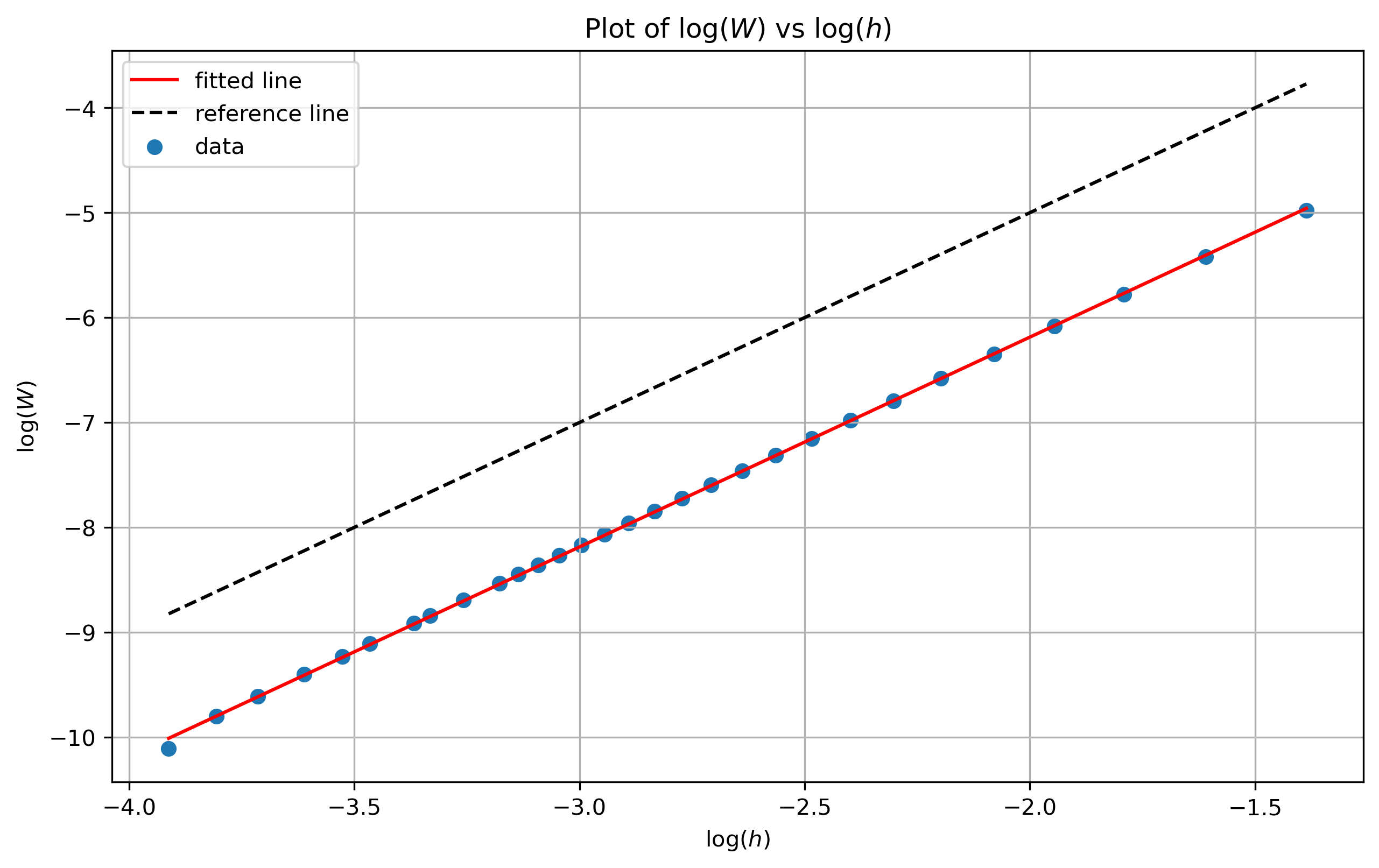
Figure 1: Log-log plot of Wasserstein distance against $h$ for the priors in a 1-D example. The reference line has a slope of 2. The slope of the fitted line is estimated to be $p=2.00$, in agreement visually with the reference line.

4.1.2 Posterior results for 1-D example

For this example we will consider a specific case of the general Bayesian inverse problem outlined in Section 2.3 which will correspond to taking the observation operator $S$ to be a pointwise evaluation operator. More specifically, we suppose that we have sensor data which correspond to noisy observations of the value of the solution $u$ at some points $\left\{y_{i}\right\}_{i=1}^{s}\subset D$. We thus take $S$ to be the operator which maps a function $g$ to the vector $Sg:=(g(y_{1}),\dots,g(y_{s}))^{T}\in\mathbb{R}^{s}$. For this choice of $S$ the update equations for the posterior means and covariances given in Eqs. 23 and 24 respectively can be simplified to a form which is more amenable to computation. These forms, for $i$ being either the symbol $\star$ or $h$, are:

$$m_{u|\mathbf{v}}^{(i)}(x) =m_{i}(x)-\mathbf{k}^{(i)}(x)^{T}B_{\epsilon,i}^{-1}(\mathbf{m}^{(i)}-\mathbf{v})$$ (38)

$$k_{u|\mathbf{v}}^{(i)}(x,y) =k_{i}(x,y)-\mathbf{k}^{(i)}(x)^{T}B_{\epsilon,i}^{-1}\mathbf{k}^{(i)}(y)$$ (39)

$$B_{\epsilon,i} :=\epsilon^{2}I+S\Sigma_{i}S^{\dagger}=\epsilon^{2}I+C_{Y,i}$$ (40)

$$\mathbf{k}^{(i)}(x) :=(k_{i}(x,y_{1}),\dots,k_{i}(x,y_{s}))^{T}$$ (41)

where $k_{u|\mathbf{v}}^{(i)}$ is the covariance function associated with $\Sigma_{u|\mathbf{v}}^{(i)}$ and where the matrix $C_{Y,i}:=S\Sigma_{i}S^{\dagger}\in\mathbb{R}^{s\times s}$ has $pq$-th entry $k_{i}(y_{p},y_{q})$. The specific sensor observations used in the experiments were obtained by simulating a trajectory from $\nu_{\star}$ evaluated at the locations $y_{1},\dots,y_{s}$.

Since we have the true posterior in an explicit form we can now demonstrate that the error bound for the full statfem posterior agrees with the error bound for linear quantities of interest from the posterior given in Theorem 4. We demonstrate this error bound for 4 different levels of sensor noise, $\epsilon=0.00005,0.0001,0.01,0.1$. These levels are chosen so that the lower values are comparable to the prior variances. We take $s=10$ sensor readings equally spaced in the interval $[0.01,0.99]\subset D$. For each level of sensor noise we again follow the argument outlined in Remark 4 and compute, for a range of sufficiently small $h$-values, an approximation of the Wasserstein distance between the two posteriors, and plot these results on a log-log scale. We take a reference grid of $N=41$ equally spaced points in $[0,1]$ to compare the covariances, and we take 28 $h$-values in $[0.025,0.25]$. With these choices we obtain the plot shown in Fig. 2 below. We also present the estimates for the slopes and intercepts of the lines of best fit in Table 1.

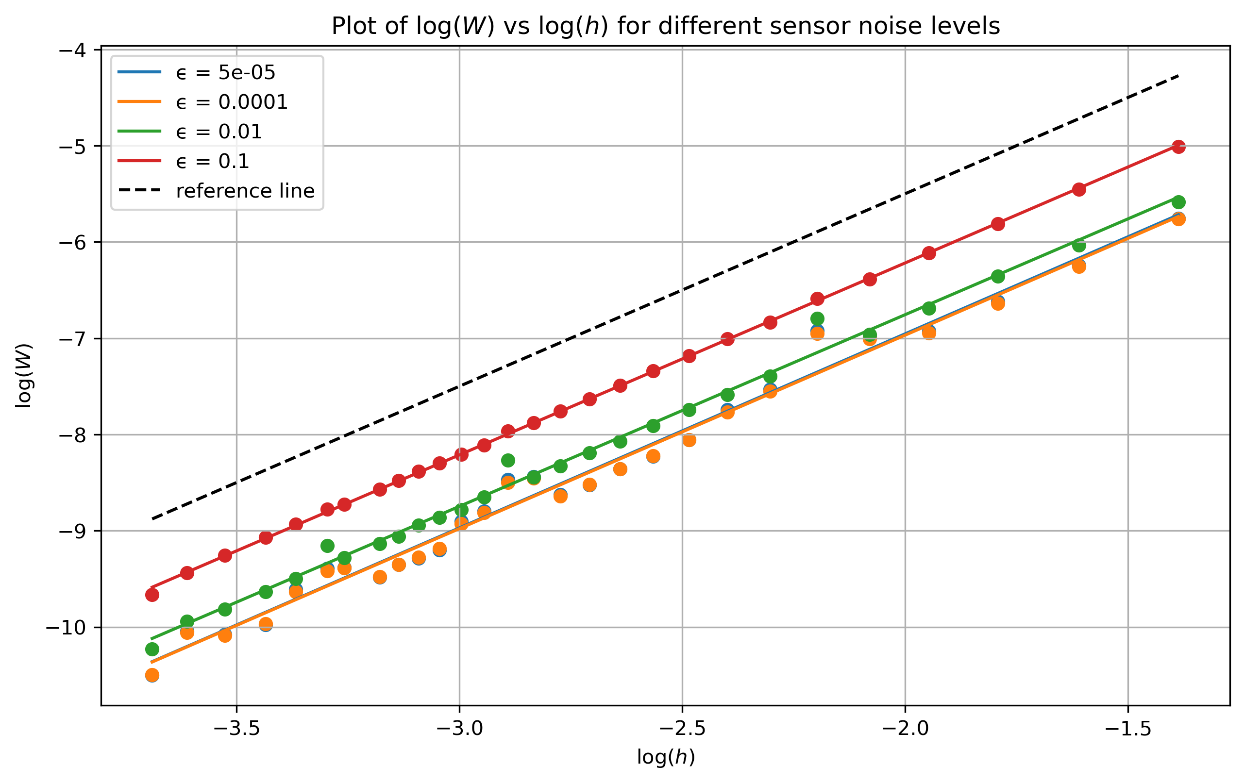
Figure 2: Log-log plot of Wasserstein distance against $h$ for the posteriors in a 1-D example for varying levels of sensor noise. The reference line has a slope of 2. Notice how the best fit lines are all parallel to the reference line.

Table 1: Estimate of slopes and intercepts for the different levels of sensor noise $\epsilon$. All of the slopes are around 2.

$\epsilon$	slope	intercept
0.00005	2.0162	-2.9227
0.00010	2.0102	-2.9486
0.01000	1.9912	-2.7739
0.10000	1.9940	-2.2309

We can see from Fig. 2 and Table 1 that we obtain lines of best-fit which are all parallel to each other, each with a slope of around $p=2$. The intercepts are slightly different for each level of sensor noise, as is to be expected since the constant in Theorem 4 depends upon $\epsilon$. These results show that the error bound for the full posterior distributions is also of order $p=2$, suggesting that it is possible to extend Theorem 4 to the Wasserstein distance between the full posteriors. Proving this is left to future research.

4.2 Two-dimensional Poisson Equation

In this section we will present a numerical example involving the following two-dimensional Poisson equation:

$$-\Delta u(x) =f(x) \quad x \in D:=[0,1]^{2}$$ (42)

$$u(x) =0 \quad x \in\partial D$$

where the forcing $f$ is distributed as,

$$f\sim\mathcal{GP}(\bar{f},k_{f})\\$$ (43)

with mean and covariance given by

$$\bar{f}(x) =1$$ (44)

$$k_{f}(x,y) =\sigma_{f}^{2}\exp\left(-\frac{\|x-y\|^{2}}{2l_{f}^{2}}\right).$$ (45)

Again we took $\sigma_{f}=0.1$ and $l_{f}=0.4$. Note that the bvp Eq. 42 is an instance of the general problem Eq. 4 with $d=2$, $D=[0,1]^{2}$, and $\kappa(x)\equiv 1$. For this problem we use the approach outlined in Remark 5 below to demonstrate the error bounds. We present the error estimates for the prior and posterior separately in the following sections.

4.2.1 Prior results for 2-D example

Following the notation of Theorem 3 we denote the statfem prior by $\nu_{h}$. Since we do not have access to the true distributions here we will need an alternative approach to that of Remark 4. This approach is outlined in the remark, taken from [1], below:

Remark 5.

When we do not have access to the true distributions we can proceed as follows. Again assuming that we have a rate of convergence, $p$, as given by Eq. 35, we can obtain an estimate as follows. First we utilise the triangle inequality to obtain,

$$W(\eta_{h},\eta_{h/2})\leq W(\eta_{h},\eta_{\star})+W(\eta_{\star},\eta_{h/2})$$ (46)

Together with Eq. 36 this yields,

$$W(\eta_{h},\eta_{h/2})=Ch^{p}+C(h/2)^{p}+\mathcal{O}(h^{p+1})$$ (47)

Similarly we have,

$$W(\eta_{h/2},\eta_{h/4})=C(h/2)^{p}+C(h/4)^{p}+\mathcal{O}(h^{p+1})$$ (48)

Dividing the two above equations yields,

$$\frac{W(\eta_{h},\eta_{h/2})}{W(\eta_{h/2},\eta_{h/4})} =\frac{Ch^{p}+C(h/2)^{p}+\mathcal{O}(h^{p+1})}{C(h/2)^{p}+C(h/4)^{p}+\mathcal{O}(h^{p+1})}$$

$$=\frac{1+2^{-p}+\mathcal{O}(h)}{2^{-p}+2^{-2p}+\mathcal{O}(h)}$$

$$=2^{p}+\mathcal{O}(h)$$ (49)

from which it follows that,

$$\operatorname{LR}(h):=\log_{2}\frac{W(\eta_{h},\eta_{h/2})}{W(\eta_{h/2},\eta_{h/4})}=p+\mathcal{O}(h)$$ (50)

From the above equation we can see that we can obtain an estimate of the rate of convergence by computing, for a range of sufficiently small $h$-values, the base-2 logarithm of the ratio $W(\eta_{h},\eta_{h/2})/W(\eta_{h/2},\eta_{h/4})$ and seeing what these logarithms tend to as $h$ gets very small. $\mathbin{\blacklozenge}$

As outlined in Remark 5 above we will compute, for a range of sufficiently small $h$-values, the base-2 logarithm of the ratio $W(\nu_{h},\nu_{h/2})/W(\nu_{h/2},\nu_{h/4})$ and see what these logarithms tend to as $h$ approaches 0. From the results of Theorem 3 we expect the logarithms to converge to 2.

We take a reference grid of $M=41^{2}=1681$ equally spaced points in $[0,1]^{2}$ to compare the covariances. We compute the logarithms for 59 $h$-values in the interval $[0.0275,0.315]$. Note that these $h$-values are not equally spaced; instead they are arranged according to a refinement strategy which was utilised for efficient use of memory. With these choices we obtain the plot shown in Fig. 3 on the next page.

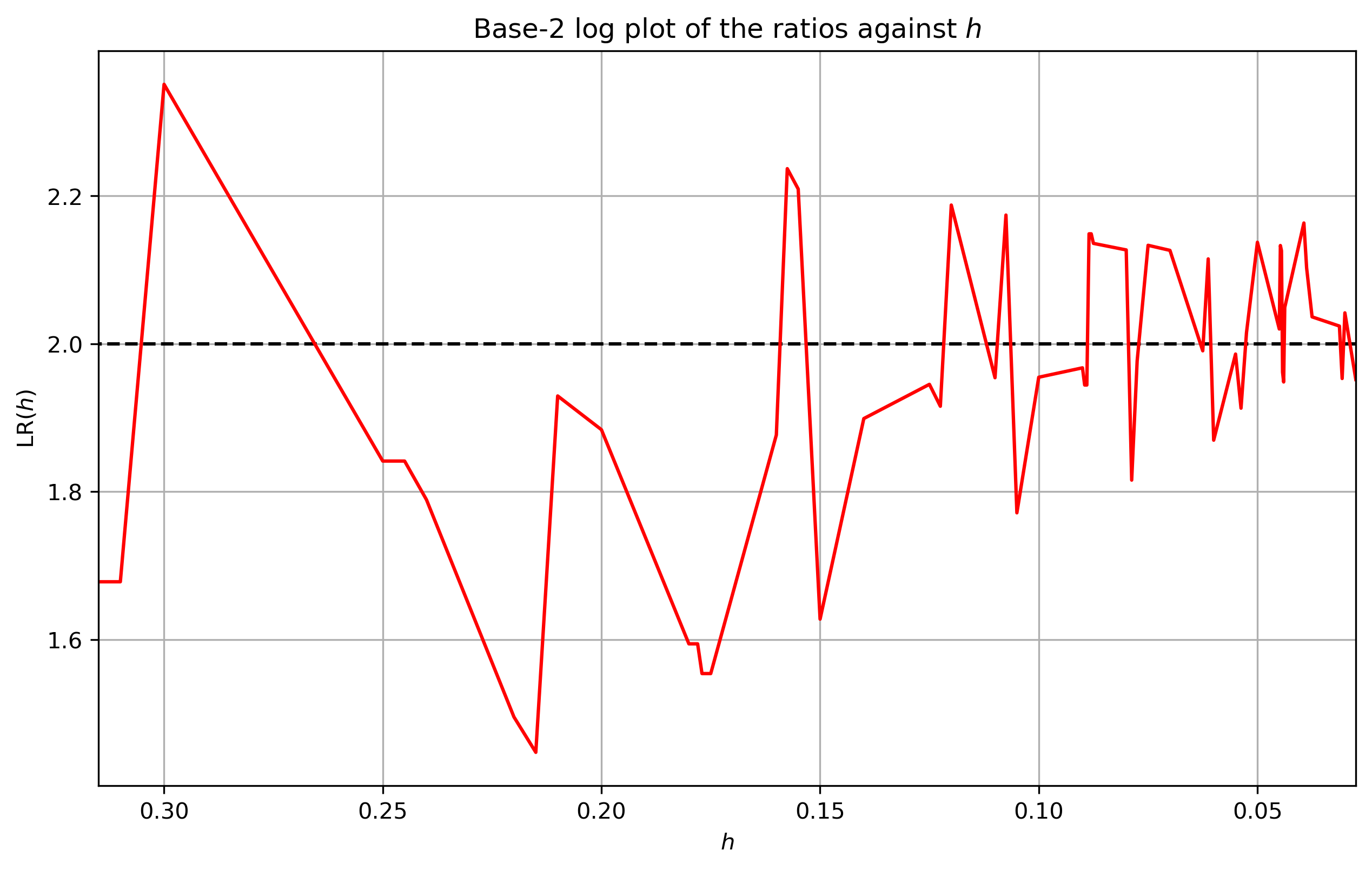
Figure 3: Plot of $\operatorname{LR}(h)$ against $h$, in the prior case, for our 2-D example.

From this plot we can see that the logarithms seem to be approaching $p=2$ as $h\to 0$, as our theory suggests. However, the results are somewhat oscillatory, which is to be expected for the approach outlined in Remark 5. Nevertheless the results seem to be oscillating around 2. To illustrate this more we smooth the above results by first discarding the results for larger $h$-values and then computing a cumulative average of the ratios before applying the base-2 logarithm. Note that this cumulative average is taken by starting with the results for large $h$ first. We take our cutoff point to be $h=0.15$. These smoothed results are shown in Fig. 4.

Figure 4: Plot of smoothed $\operatorname{LR}(h)$ for $h\leq 0.15$, in the prior case. The horizontal axis indicates the smallest $h$ value taken in the cumulative averages.

From Fig. 4 we can see that by discarding the values corresponding to $h>0.15$ the base-2 logarithms of the rolling averages converge to a value slightly greater than $2$. The final logarithm for these rolling averages is $p=2.02$ (to 2 decimal places). Thus, we obtain results in close agreement with Theorem 3.

4.2.2 Posterior results for 2-D example

For this example we will consider the same specific case of the general Bayesian inverse problem which we chose in Section 4.1.2. That is, we will again take the observation operator $S$ to be an evaluation operator. Since we do not have the true prior in an explicit form, we also do not have the true posterior and as such we will utilise the argument in Remark 5 to demonstrate the statfem posterior error bound. To generate sensor readings, since we do not have access to the true prior, we instead simulated trajectories from the statfem prior with a very fine grid of mesh size $h=1/120$.

We take a reference grid of $M=41^{2}=1681$ equally spaced points in $[0,1]^{2}$ to compare the covariances. We set the sensor noise level to $\epsilon=0.001$ and take $s=25$ sensor readings equally spaced in $[0.01,0.99]^{2}\subset D$. The level of sensor noise is chosen to be comparable to the prior variances. We follow the notation of Theorem 4 and denote the statfem posterior by $\tilde{\nu}_{h}$. We compute the logarithms $\log_{2}\left(W(\tilde{\nu}_{h},\tilde{\nu}_{h/2})/W(\tilde{\nu}_{h/2},\tilde{\nu}_{h/4})\right)$ for 53 $h$-values in the interval $[0.03125,0.315]$, which are spread out according to the refinement strategy mentioned in Section 4.2.1. With these choices we obtain the plot shown in Fig. 5 below.

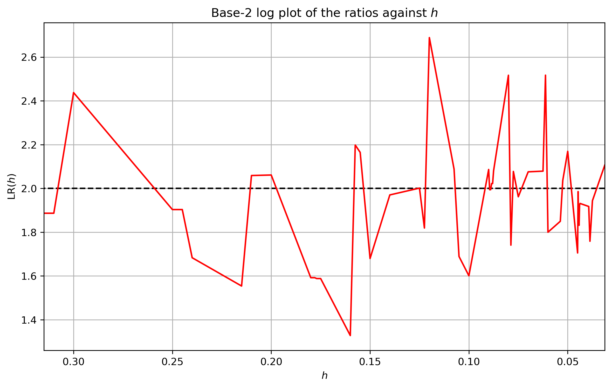
Figure 5: Plot of $\operatorname{LR}(h)$ against $h$, in the posterior case, for our 2-D example.

From this plot we can see that the logarithms seem to be approaching $p=2$ as $h$ gets small. However, just as in Section 4.2.1, the results are oscillatory but seem to be oscillating around $p=2$. We will thus smooth the results as explained in Section 4.2.1. We again take the cutoff point to be $h=0.15$. These smoothed results are shown in Fig. 6 on the next page. From this figure we can see that by discarding the values corresponding to $h>0.15$ the base-2 logarithms of the rolling averages converge to a value slightly greater than 2. The final logarithm of these rolling averages is $p=2.00$ (to 2 decimal places). Thus, just as in the 1D example we see results which suggest that it is possible to extend Theorem 4 to the case of the full posteriors.

Figure 6: Plot of smoothed $\operatorname{LR}(h)$ for $h\leq 0.15$, in the posterior case. The horizontal axis indicates the smallest $h$ value taken in the cumulative averages.

4.3 Distribution of the maximum

In this section we will present a numerical experiment involving the same one-dimensional Poisson equation Eq. 27. The forcing $f$ will follow the same distribution as given in Eq. 28, but we will adjust the kernel lengthscale to be $l_{f}=0.01$ instead, as with a larger length-scale the maximum of the statfem prior and posterior were found to converge too quickly to demonstrate interesting behaviour. Since the solution, $u$, is random the maximum, $\max_{x\in[0,1]}u(x)$, is a univariate random variable. Since taking the maximum is not a linear functional we have no guarantees that the distribution of the maximum will be Gaussian. More importantly our results from Theorem 4 will not necessarily hold for this example.

We will investigate the errors for the true and statfem prior/posterior distributions for the maximum via a Monte Carlo approach as we now outline in the following remark.

Remark 6.

Let $\eta_{\star},\eta_{h}$ denote the true and statfem prior (or posterior) for the maximum of $u$ respectively. We are interested in investigating the rate of convergence of $W(\eta_{\star},\eta_{h})$ as $h\rightarrow 0$. This is done as follows: in both the prior and posterior case we will first fix a reference grid $\{\tilde{x_{i}}\}_{i=1}^{N}$ and obtain samples of trajectories of the solution on this grid from the true distribution. We then take the maximum values of these trajectories to obtain an (approximate) sample from the true distribution for $\max_{x\in[0,1]}u(x)$. For a range of $h$-values we will then simulate trajectories of the solution on the same reference grid from the statfem distribution and then take the maximum values of these to obtain an (approximate) sample for the statfem case. We will then compute an approximation of the Wasserstein distance $W(\eta_{\star},\eta_{h})$ by computing the Wasserstein distance between these two empirical distributions for each $h$-value by utilising the Python package POT [13]. We then investigate the rate of convergence as outlined previously in Remark 4. $\mathbin{\blacklozenge}$

The results for the statfem priors and posteriors will be presented separately in the following sections.

4.4 Prior results for maximum example

As outlined in Remarks 6 and 4, we compute, for a range of sufficiently small $h$-values, a Monte Carlo approximation to the Wasserstein distance between the two priors for the maximum. We take a reference grid of $N=100$ equally spaced points in $[0,1]$ and $30$ $h$-values in $[0.02,0.25]$. We simulate $1000$ trajectories from both priors to obtain approximate samples of the maximum. With these choices we obtain the plot shown in Fig. 7 below. From this plot we can see that the we indeed have convergence of the Wasserstein distance for this non-linear quantity of interest to $0$, but at a different rate than that given in Theorem 3. The slope is estimated to be $p=1.35$ (to 2 decimal places).

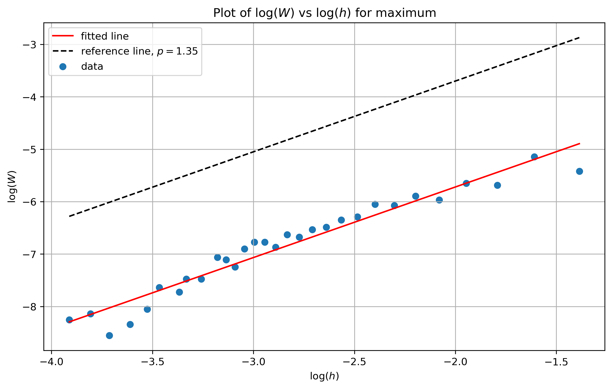
Figure 7: Log-log plot of Wasserstein distance against $h$ for the priors for the maximum. The reference line has a slope of 1.35. The slope of the fitted line is estimated to be $p=1.35$, in agreement visually with the reference line.

4.5 Posterior results for maximum example

For the posterior case we take a reference grid of $N=41$ equally spaced points in $[0,1]$ to simulate $1000$ trajectories and $30$ $h$-values in $[0.02,0.25]$. We take $s=10$ sensor readings equally spaced in the interval $[0.01,0.99]$. This is repeated for $4$ different levels of sensor noise, $\epsilon=0.0001,0.0005,0.001,0.01$, again chosen so that the lower noise levels are comparable to the prior variances. For each level of noise we follow the argument outlined in Remarks 6 and 4. With these choices we obtain the plot shown in Fig. 8 on the next page. We also present the estimates for the slopes and intercepts of the lines of best fit in Table 2.

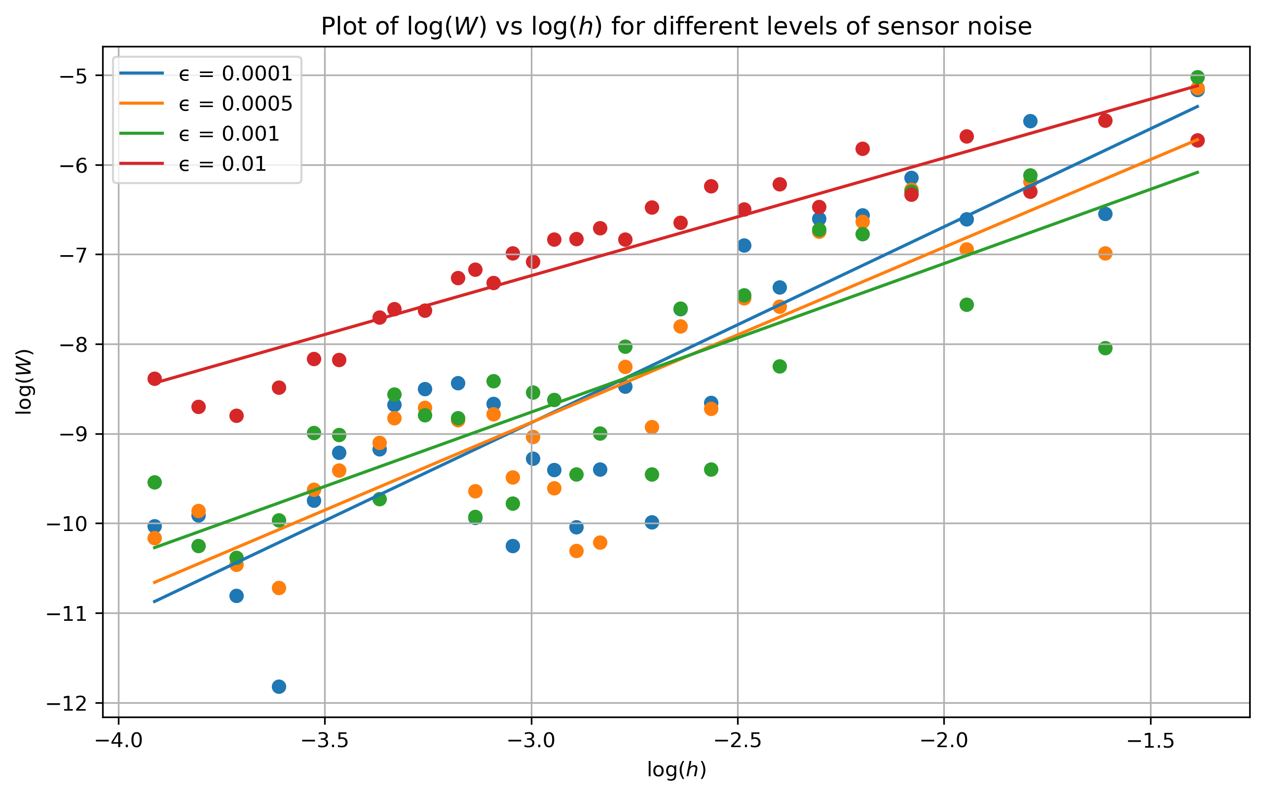
Figure 8: Log-log plot of Wasserstein distance against $h$ for the posteriors for the maximum for different levels of sensor noise.

Table 2: Estimate of slopes and intercepts for the different levels of sensor noise $\epsilon$.

$\epsilon$	slope	intercept
0.00010	2.1862	-2.3203
0.00050	1.9552	-3.0104
0.00100	1.6573	-3.7885
0.01000	1.3131	-3.2989

From Fig. 8 and Table 2 we can see that for each level of sensor noise we do indeed have convergence to $0$ as $h$ goes to 0. However, we observe that the rate is not always the same as that given in Theorem 4. From Table 2 it is particularly clear that as the sensor noise level decreases the rate of convergence increases. In particular, for $\epsilon=0.0001,0.0005$ we have rates around $p=2$, similar to the case of linear quantities of interest. We hypothesise that this is because as the sensor noise decreases the posterior distribution concentrates more as the solution is better identified and this, combined with the fact that we take sensor readings close to the where the true prior mean Eq. 33 has a maximum, forces the maximum of the simulated trajectories to always be at the argmax of the prior mean in the exact case, i.e. at $x=0.5$. Thus for very low levels of sensor noise taking the maximum of the posterior draws is almost identical to evaluating the solution at $x=0.5$; such an evaluation is a linear quantity of interest and so one would expect the results from Theorem 4 to hold.

5 Conclusion

In this paper we have provided detailed error analysis for the statfem method first introduced in [14, 15] for the case of spatial elliptic bvp. In particular, we have proven that the statfem prior converges, with respect to the Wasserstein-2 distance, to the true prior at a rate of $\mathcal{O}(h^{2})$. We also showed that in the posterior case linear quantities of interest are also controlled at a rate of $\mathcal{O}(h^{2})$. In both settings, the choice of the Wasserstein distance provides a convenient metric in which to quantify the error introduced through discretisation. Numerical experiments demonstrating the theoretical results on standard fem test problems were then presented. These demonstrated the rates for the prior theory, while also showcasing that it may be possible to extend the posterior results to the full distribution as opposed to just linear quantities of interest. An example involving a non-linear quantity of interest was also presented, showcasing an example which lies out of the remit of our theory.

Several possible avenues for future work present themselves. The first would be to prove error bounds for the full posterior distributions, extending Theorem 4. Another avenue would be to provide similar error analysis for statfem in the case of time-dependent problems. It would also be interesting to see if similar error bounds can be proven for distributions utilising approximations other than fem. Generalising the results to utilise Wasserstein-$p$ distance, for $p>2$, would also be an interesting goal, as this will allow one to have even more control over other aspects of the distribution such as quantiles and extrema, which is especially important for risk-assessment applications.

See pages - of supplement

References

- [1] Verifying numerical convergence rates. Technical report, KTH. https://www.csc.kth.se/utbildning/kth/kurser/DN2255/ndiff13/ConvRate.pdf.
- Aldosary et al. [2018] M. Aldosary, J. Wang, and C. Li. Structural reliability and stochastic finite element methods. Engineering Computations, 2018.
- Bogachev [1998] V. I. Bogachev. Gaussian measures. Number 62. American Mathematical Soc., 1998.
- Chkrebtii et al. [2016] O. A. Chkrebtii, D. A. Campbell, B. Calderhead, M. A. Girolami, et al. Bayesian solution uncertainty quantification for differential equations. Bayesian Analysis, 11(4):1239–1267, 2016.
- Cockayne et al. [2016] J. Cockayne, C. Oates, T. Sullivan, and M. Girolami. Probabilistic numerical methods for partial differential equations and bayesian inverse problems. arXiv preprint arXiv:1605.07811, 2016.
- Cockayne et al. [2019] J. Cockayne, C. J. Oates, T. J. Sullivan, and M. Girolami. Bayesian probabilistic numerical methods. SIAM Review, 61(4):756–789, 2019.
- Conrad et al. [2017] P. R. Conrad, M. Girolami, S. Särkkä, A. Stuart, and K. Zygalakis. Statistical analysis of differential equations: introducing probability measures on numerical solutions. Statistics and Computing, 27(4):1065–1082, 2017.
- Cotter et al. [2009] S. L. Cotter, M. Dashti, J. C. Robinson, and A. M. Stuart. Bayesian inverse problems for functions and applications to fluid mechanics. Inverse problems, 25(11):115008, 2009.
- Cuesta-Albertos et al. [1996] J. Cuesta-Albertos, C. Matrán-Bea, and A. Tuero-Diaz. On lower bounds for the l2-wasserstein metric in a hilbert space. Journal of Theoretical Probability, 9(2):263–283, 1996.
- Da Prato and Zabczyk [2014] G. Da Prato and J. Zabczyk. Stochastic equations in infinite dimensions. Cambridge university press, 2014.
- Dowson and Landau [1982] D. Dowson and B. Landau. The fréchet distance between multivariate normal distributions. Journal of multivariate analysis, 12(3):450–455, 1982.
- Evans [2010] L. C. Evans. Partial differential equations. American Mathematical Society, Providence, R.I., 2010. ISBN 9780821849743 0821849743.
- Flamary et al. [2021] R. Flamary, N. Courty, A. Gramfort, M. Z. Alaya, A. Boisbunon, S. Chambon, L. Chapel, A. Corenflos, K. Fatras, N. Fournier, L. Gautheron, N. T. Gayraud, H. Janati, A. Rakotomamonjy, I. Redko, A. Rolet, A. Schutz, V. Seguy, D. J. Sutherland, R. Tavenard, A. Tong, and T. Vayer. Pot: Python optimal transport. Journal of Machine Learning Research, 22(78):1–8, 2021. URL http://jmlr.org/papers/v22/20-451.html.
- Girolami et al. [2019] M. Girolami, A. Gregory, G. Yin, and F. Cirak. The statistical finite element method. arXiv preprint arXiv:1905.06391, 2019.
- Girolami et al. [2021] M. Girolami, E. Febrianto, G. Yin, and F. Cirak. The statistical finite element method (statFEM) for coherent synthesis of observation data and model predictions. Computer Methods in Applied Mechanics and Engineering, 375:113533, Mar. 2021. 10.1016/j.cma.2020.113533. URL https://doi.org/10.1016/j.cma.2020.113533.
- Grisvard [2011] P. Grisvard. Elliptic problems in nonsmooth domains. SIAM, 2011.
- Hennig et al. [2015] P. Hennig, M. A. Osborne, and M. Girolami. Probabilistic numerics and uncertainty in computations. Proceedings of the Royal Society A: Mathematical, Physical and Engineering Sciences, 471(2179):20150142, 2015.
- Larsson and Thomée [2008] S. Larsson and V. Thomée. Partial differential equations with numerical methods, volume 45. Springer Science & Business Media, 2008.
- Lindgren et al. [2011] F. Lindgren, H. Rue, and J. Lindström. An explicit link between gaussian fields and gaussian markov random fields: the stochastic partial differential equation approach. Journal of the Royal Statistical Society: Series B (Statistical Methodology), 73(4):423–498, 2011.
- Lord et al. [2014] G. J. Lord, C. E. Powell, and T. Shardlow. An introduction to computational stochastic PDEs, volume 50. Cambridge University Press, 2014.
- Martino and Riebler [2014] S. Martino and A. Riebler. Integrated nested laplace approximations (inla). Wiley StatsRef: Statistics Reference Online, pages 1–19, 2014.
- Masarotto et al. [2019] V. Masarotto, V. M. Panaretos, and Y. Zemel. Procrustes metrics on covariance operators and optimal transportation of gaussian processes. Sankhya A, 81(1):172–213, 2019.
- Matthies et al. [1997] H. G. Matthies, C. E. Brenner, C. G. Bucher, and C. Guedes Soares. Uncertainties in probabilistic numerical analysis of structures and solids-stochastic finite elements. Structural Safety, 19(3):283–336, 1997. ISSN 0167-4730. https://doi.org/10.1016/S0167-4730(97)00013-1. URL https://www.sciencedirect.com/science/article/pii/S0167473097000131. Devoted to the work of the Joint Committee on Structural Safety.
- Olkin and Pukelsheim [1982] I. Olkin and F. Pukelsheim. The distance between two random vectors with given dispersion matrices. Linear Algebra and its Applications, 48:257–263, 1982.
- Owhadi [2015] H. Owhadi. Bayesian numerical homogenization. Multiscale Modeling & Simulation, 13(3):812–828, 2015.
- Rasmussen [2006] C. E. Rasmussen. Gaussian processes for machine learning. MIT Press, 2006.
- Scheuerer [2010] M. Scheuerer. Regularity of the sample paths of a general second order random field. Stochastic Processes and their Applications, 120(10):1879–1897, 2010.
- Sigrist et al. [2015] F. Sigrist, H. R. Künsch, and W. A. Stahel. Stochastic partial differential equation based modelling of large space–time data sets. Journal of the Royal Statistical Society: Series B: Statistical Methodology, pages 3–33, 2015.
- Stefanou [2009] G. Stefanou. The stochastic finite element method: Past, present and future. Computer Methods in Applied Mechanics and Engineering, 198(9):1031–1051, 2009. ISSN 0045-7825. https://doi.org/10.1016/j.cma.2008.11.007. URL https://www.sciencedirect.com/science/article/pii/S0045782508004118.
- Strang and Fix [1973] G. Strang and G. J. Fix. An analysis of the finite element method. Journal of Applied Mathematics and Mechanics, 1973.
- Stuart [2010] A. M. Stuart. Inverse problems: a bayesian perspective. Acta numerica, 19:451–559, 2010.
- Sudret and Der Kiureghian [2000] B. Sudret and A. Der Kiureghian. Stochastic finite element methods and reliability: a state-of-the-art report. Department of Civil and Environmental Engineering, University of California …, 2000.
- Tronarp et al. [2019] F. Tronarp, H. Kersting, S. Särkkä, and P. Hennig. Probabilistic solutions to ordinary differential equations as nonlinear bayesian filtering: a new perspective. Statistics and Computing, 29(6):1297–1315, 2019.
- Xiu [2010] D. Xiu. Numerical methods for stochastic computations: a spectral method approach. Princeton university press, 2010.
- Zhang and Karniadakis [2017] Z. Zhang and G. Karniadakis. Numerical methods for stochastic partial differential equations with white noise. Springer, 2017.