SDSS J1451+2709 a normal blue quasar but mis-classified as a HII galaxy in the BPT diagram by flux ratios of narrow emission lines
Abstract
In the manuscript, we discuss properties of SDSS J1451+2709, a normal blue quasar but mis-classified as a HII galaxy in the BPT diagram (called as a mis-classified quasar). The emission lines around H and around H are well measured by different model functions with broad Balmer lines described by Gaussian or Lorentz functions, in the SDSS spectrum in 2007 and in the KPNO spectrum in 1990. After considering variations of broad emission lines, different model functions lead to different determined fluxes of narrow emission lines, but the different narrow emission line flux ratios lead the SDSS J1451+2709 as a HII galaxy in the BPT diagram. In order to explain the unique properties of the mis-classified quasar SDSS J1451+2709 in the BPT diagram, two methods are proposed, the starforming contributions and compressed NLRs with high electron densities near to critical densities of forbidden emission lines. Unfortunately, the two methods cannot be preferred in the SDSS J1451+2709, further efforts are necessary to find the physical origin of the unique properties of the mis-classified quasar SDSS J1451+2709 in the BPT diagram. Meanwhile, there are not quite different long-term variabilities of SDSS J1451+2709 from the normal quasars. The mis-classified quasar SDSS J1451+2709, an extremely unique case or a special case among the normal quasars, could provide further clues on the applications of BPT diagrams to the normal broad line AGN and to narrow emission line objects, indicating part of narrow emission line HII galaxies actually harbouring central AGN activities.
keywords:
galaxies:active - galaxies:nuclei - quasars:emission lines - galaxies:Seyfert1 Introduction
SDSS J1451+2709 (= SDSS J145108+270926.92, also known as PG 1448+273) is always a common broad line blue quasar, since its first reported in the PG (Palomar-Green) quasar sample of Boroson & Green (1992). As the shown spectra in Fig. 1 from SDSS (Sloan Digital Sky Survey) (the SDSS spectrum) and from the KPNO (Kitt Peak National Observatory) 2.1m telescope (Boroson & Green, 1992) (the KPNO spectrum), SDSS J1451+2709 is an un-doubtfully normal broad line blue quasar (a type-1 AGN). However, based on flux ratios of narrow emission lines well discussed in Section 2 and in Section 3, SDSS J1451+2709 can be well classified as a HII galaxy instead of an AGN in the BPT diagram (Baldwin, Phillips & Terlevich, 1981; Kewley et al., 2001; Kauffmann et al., 2003; Kewley et al., 2006, 2013a, 2019; Zhang et al., 2020). Therefore, in the manuscript, some special properties of SDSS J1451+2709 is studied.
Type-1 AGN (broad line Active Galactic Nuclei) and Type-2 AGN (narrow line AGN) having the similar properties of intrinsic broad and narrow emission lines, in the framework of the commonly accepted and well-known constantly being revised Unified Model (Antouncci, 1993; Ramos et al., 2011; Netzer, 2015; Audibert et al., 2017; Balokovic et al., 2018; Brown et al., 2019; Kuraszkiewicz et al., 2021) which has been successfully applied to explain different features between Type-1 and Type-2 AGN in many different ways. In other words, central broad line regions (BLRs) with distances of tens to hundreds of light-days (Kaspi et al., 2000, 2005; Bentz et al., 2006, 2009; Denney et al., 2010; Bentz et al., 2013; Fausnaugh et al., 2017) to central black holes (BHs) are totally obscured by central dust torus (or other high density dust clouds), leading to no broad emission lines (especially in optical band) in observed spectra of Type-2 AGN. However, much extended narrow line regions (NLRs) with distances of hundreds to thousands of pcs (parsecs) to central BHs (Fischer et al., 2013; Hainline et al., 2014; Fischer et al., 2017; Sun et al., 2017) lead to the similar observed properties of narrow emission lines in Type-1 AGN and in Type-2 AGN, such as the strong linear correlation between the AGN power-law continuum luminosity and the [O iii]Å line luminosity (Zakamska et al., 2003; Shen et al., 2011; Heckman & Best, 2014; Zhang & Feng, 2017). Type-2 AGN are intrinsically like Type-1 AGN expected by the Unified Model, strongly indicating that central AGN activities not only can be determined by narrow emission line properties but also can be determined by broad emission line properties.
For an emission line object, there are two main methods applied to classify whether the object is an AGN or not? On the one hand, for a broad emission line object, through the clear spectroscopic features of broad emission lines and the strong blue power-low continuum emissions, a broad emission line object can be conveniently and directly classified as a type-1 AGN. On the other hand, for a narrow emission line object, the well-known BPT diagrams (Baldwin, Phillips & Terlevich, 1981; Kauffmann et al., 2003; Kewley et al., 2006, 2013a, 2013b, 2019; Zhang et al., 2020) can be conveniently applied to determine whether the object is a Type-2 AGN (narrow line AGN) or a HII galaxy by properties of flux ratios of narrow emission lines. If there were similar intrinsic central activity properties, we could expect that the flux ratios of narrow emission lines for broad line objects (type-1 AGN) can also lead the broad line AGN to be well classified as AGN in the BPT diagrams. However, if there were some special bright type-1 AGN (called as mis-classified AGN in the manuscript), of which flux ratios of narrow emission lines lead the broad line AGN classified as HII galaxies in the BPT diagrams, it would be very interesting to check properties of the special mis-classified AGN, which could probably provide further clues on unique properties of central emission structures.
Not similar as standard narrow emission line AGN (type-2 AGN), there are more complicated line profiles of emission lines in broad line AGN, not only narrow emission components but also broad emission components in the spectrum. In some cases, the broad emission lines have line width (second moment) around several hundreds of kilometers per second, gently wider than extended components of forbidden/permitted emission lines, such as the commonly known extended components in [O iii]Å doublet discussed in Greene & Ho (2005); Shen et al. (2011); Zhang & Feng (2017); Zhang (2021a, b). It would be more difficult to determine narrow line flux ratios in some broad line AGN, until the narrow emission components can be well measured and confirmed. Therefore, variability properties of emission components in multi-epoch spectra of broad line AGN should be efficient to determine the emission regions in NLRs or in BLRs.
In the manuscript, among the SDSS pipeline classified low-redshift quasars () (Richards et al., 2002; Ross et al., 2012; Peters et al., 2015; Lyke et al., 2020), SDSS J1451+2709 (PG 1448+273) is collected as the target, because of the following two main reasons. On the one hand, SDSS J1451+2709 has its type classified as a HII galaxy in the BPT diagram by flux ratios of narrow emission lines as well discussed in the following sections. On the other hand, SDSS J1451+2709 has two-epoch spectra observed in SDSS in 2007 and observed by the KPNO telescope in 1990, which will provide robust evidence to confirm the more reasonable flux ratios of narrow emission lines.
The manuscript is organized as follows. Section 2 shows the properties of the spectroscopic emission lines by different model functions with different considerations. Section 3 shows the properties of SDSS J1451+2709 in the BPT diagram. Section 4 discusses the probable physical origin of the unique properties of the mis-classified quasar SDSS J1451+2709 in the BPT diagram. Section 5 shows the long-term variability properties of the mis-classified quasar SDSS J1451+2709. Section 6 shows the further implications. Section 7 gives our final summaries and conclusions. And in the manuscript, the cosmological parameters of , and have been adopted.

2 Properties of spectroscopic emission lines of SDSS J1451+2709
Fig. 1 shows the SDSS spectrum of SDSS J1451+2709 observed in 2007 and the KPNO spectrum observed in 1990, with apparent broad emission lines and blue power-law continuum emissions. It is clear that SDSS J1451+2709 is an un-doubtfully broad line blue quasar. In order to show the classification of SDSS J1451+2709 by flux ratios of narrow emission lines in the BPT diagram, the following emission line fitting procedures with different model functions are applied to describe the emission lines of SDSS J1451+2709, especially the emission lines of narrow H, narrow H, [O iii]Å doublet and [N ii]Å doublet which will be applied in the following BPT diagram.
Here, we mainly consider the emission lines around H and around H (rest wavelength from 4400 to 5600Å and from 6250 to 6950Å), which are fitted simultaneously by the following two different kinds of model functions. The fitting procedure is very similar as what we have done in Zhang & Feng (2016, 2017); Zhang (2021a, b).
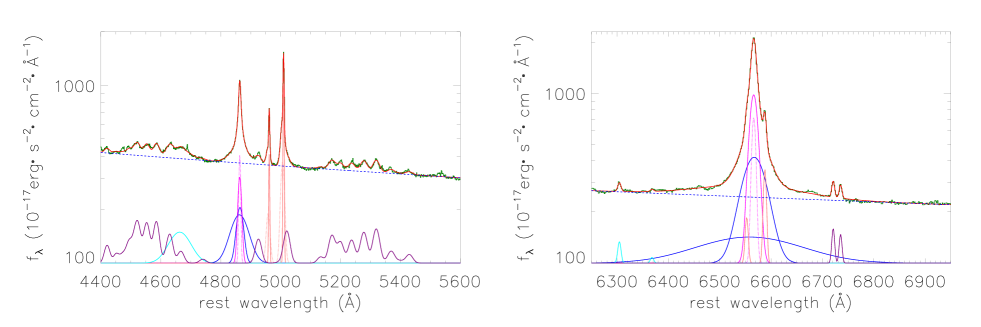
For model A, the model functions are mainly based on Gaussian functions applied to describe the emission lines as follows. Two narrow plus two broad Gaussian functions applied to describe the core and extended components of [O iii]Å doublet. Here, the broad Gaussian function means its second moment larger than the narrow Gaussian function, no restrictions on the lower limit of the second moment of the broad Gaussian function. One narrow and one broad Gaussian functions applied to describe the narrow H. One narrow and one broad Gaussian functions applied to describe the narrow H. Two111More than two broad Gaussian functions have also been applied to describe the broad Balmer lines, however, the third or more broad Gaussian components are not necessary, because of the corresponding determined model parameters smaller than their uncertainties. broad Gaussian functions are applied to describe the broad H. Two broad Gaussian functions are applied to describe the broad H. Two222It is not necessary to consider extended components in [O i], [S ii] and [N ii] doublets. If additional Gaussian components are applied to describe probable extended components in the doublets, the determined line fluxes of the extended components are near to zero and smaller than determined uncertainties. Therefore, in the manuscript, besides the [O iii] doublet, there are no considerations on extended components of the forbidden emission lines. narrow Gaussian functions are applied to describe the [O i]Å doublet. Two narrow Gaussian functions are applied to describe the [S ii]Å doublet. Two narrow Gaussian functions are applied to describe the [N ii]Å doublet. One broad Gaussian function is applied to describe the broad He ii line. The broadened optical Fe ii template in Kovacevic et al. (2010) is applied to describe the optical Fe ii emission features. One power law component is applied to describe the AGN continuum emissions underneath the emission lines around H. One power law component is applied to describe the AGN continuum emissions underneath the emission lines around H. For the model parameters in model A, the following restrictions are accepted. First, the flux of each Gaussian component is not smaller than zero. Second, the flux ratio of the [O iii] doublet ([N ii] doublet) is fixed to the theoretical value 3. Third, the Gaussian components of each forbidden line doublet have the same redshift and the same line width in velocity space. There are no further restrictions on the parameters of Balmer emission lines.
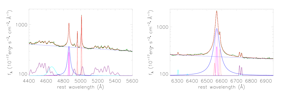
For model B, the model functions are similar as the ones in model A, but the broad H (H) is described by only one broad Lorentz function. And the same restrictions are accepted to the model parameters in model B. The main objective to consider Lorentz function to describe the broad Balmer lines is as follows. Not similar as Gaussian function, Lorentz function always has sharp peak which can lead to more smaller measured fluxes of narrow Balmer lines, which will have positive effects on the classifications as HII galaxies by flux ratios of narrow emission lines in BPT diagram, which will be discussed in the following section. Here, we do not discuss the physical origin of Lorentz function described broad Balmer emission components, but the Lorentz function described broad Balmer emission components can lead to more reliable results on the SDSS J1451+2709 being classified as a HII galaxy in the BPT diagram.
Through the Levenberg-Marquardt least-squares minimization technique, the emission lines around H and around H can be well measured. The best fitting results are shown in Fig. 2 with (summed squared residuals divided by degree of freedom) by model A, and in Fig 3 with by model B. The line parameters of each Gaussian component of narrow emission lines, Gaussian and Lorentz describe broad Balmer lines, and the power law continuum emissions are listed in Table 1.
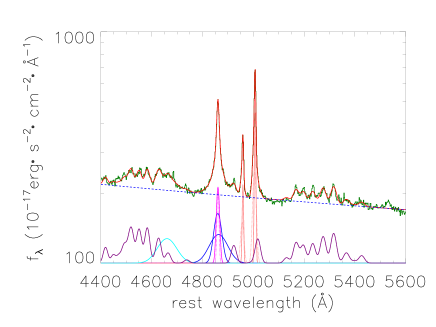
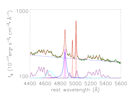
Based on the similar model functions in model A and in model B, but with no considerations on emission lines around H (not covered in the KPNO spectrum), the emission lines around H in the KPNO long-slit spectrum in 1990 can be also well measured. The best fitting results are shown in the top panel of Fig. 4 with broad H described by two broad Gaussian functions, and in the bottom panel of Fig 4 with broad H described by one broad Lorentz function. The line parameters of each Gaussian component of narrow emission lines, Gaussian and Lorentz described broad H and the power law continuum emissions are also listed in Table 1. Here, due to loss of uncertainty information of the KPNO spectrum collected from NED (NASAIPAC Extragalactic Database (http://ned.ipac.caltech.edu/results/NEDspectra_output_127_page1_details.html#PG_1448+273_2), no uncertainties of determined model parameters are listed in Table 1 for the spectroscopic features in 1990.
| name | flux | flux | ||||
| Emission lines in the SDSS spectrum | ||||||
| Gaussian Broad Balmer lines | Lorentz Broad Balmer lines | |||||
| H | 4862.770.74 | 28.861.52 | 6.280.46 | 4863.890.19 | 29.151.36 | 12.520.22 |
| H | 4864.270.48 | 11.211.65 | 2.960.45 | … | … | … |
| He ii | 4662.791.33 | 34.881.24 | 4.300.15 | 4664.241.33 | 34.511.21 | 4.280.15 |
| H | 4863.610.07 | 5.980.23 | 3.060.69 | 4863.390.13 | 4.380.25 | 2.750.43 |
| H | 4863.700.08 | 2.830.17 | 2.160.32 | 4863.960.17 | 2.210.29 | 1.060.35 |
| [O iii]Å(N) | 5010.040.03 | 1.640.03 | 3.810.08 | 5010.040.03 | 1.640.03 | 3.770.08 |
| [O iii]Å(E) | 5006.490.15 | 6.060.11 | 4.080.09 | 5006.530.14 | 6.020.11 | 4.050.09 |
| H | 6557.682.18 | 98.883.84 | 10.180.32 | 6566.46 0.14 | 31.191.31 | 40.241.12 |
| H | 6566.820.25 | 23.180.45 | 18.610.52 | … | … | … |
| H | 6565.870.12 | 8.070.39 | 17.850.76 | 6565.570.18 | 5.910.34 | 11.221.13 |
| H | 6565.990.09 | 3.830.19 | 6.011.02 | 6566.340.23 | 2.990.39 | 2.230.94 |
| [N ii]Å | 6587.920.12 | 2.830.12 | 1.830.09 | 6587.760.11 | 2.770.13 | 1.730.09 |
| [O i]Å | 6304.370.33 | 3.040.34 | 0.260.03 | 6304.320.33 | 2.520.34 | 0.200.02 |
| [O i]Å | 6367.880.35 | 3.070.36 | 0.060.02 | 6367.830.33 | 2.540.34 | 0.050.02 |
| [S ii]Å | 6720.710.13 | 2.610.13 | 0.390.02 | 6720.680.14 | 2.740.14 | 0.430.02 |
| [S ii]Å | 6735.090.14 | 2.610.14 | 0.310.02 | 6735.060.14 | 2.750.14 | 0.330.02 |
| pow H | ||||||
| pow H | ||||||
| Emission lines in the KPNO spectrum | ||||||
| Gaussian Broad Balmer lines | Lorentz Broad Balmer lines | |||||
| H | 4863.21 | 34.53 | 2.84 | 4860.81 | 30.69 | 7.09 |
| H | 4860.12 | 15.03 | 2.36 | … | … | … |
| He ii | 4659.86 | 36.11 | 2.49 | 4661.11 | 35.71 | 2.47 |
| H | 4860.97 | 6.24 | 1.56 | |||
| H | 4860.88 | 3.73 | 1.13 | 4860.91 | 4.14 | 1.74 |
| [O iii]Å(N) | 5007.04 | 2.58 | 2.34 | 5007.05 | 2.56 | 2.32 |
| [O iii]Å(E) | 5004.46 | 6.46 | 2.39 | 5004.52 | 6.35 | 2.36 |
| pow H | ||||||
Note: The first column shows the information of emission component listed. [O iii]Å(E) and [O iii]Å(N) mean the extended and the core component of [O iii]Å. H and H mean the extended and the core component of narrow H, and H and H mean the extended and the core component of narrow H. The ’pow H’ and the ’pow H’ mean the power law continuum emissions around H and around H, respectively. The second column to the fourth column show the line parameters of central wavelength in unit of Å, second moment in unit of Å and line flux in unit of of the determine components by Model A with two broad Gaussian functions (H, H and H, H) applied to describe the broad Balmer lines. The fifth column to the seventh column show the line parameters of the determine components by Model B with one broad Lorentz function (H, H) applied to describe the broad Balmer lines.
It is clear that different model functions lead to quite different line parameters of narrow Balmer emission lines but similar line parameters of [O iii] and [N ii] doublets, which will lead to quite different flux ratios of [O iii] to narrow H and [N ii] to narrow H, Therefore, before to discuss properties of SDSS J1451+2709 in the BPT diagram, it is necessary to discuss which emission component of Balmer line emissions is actually from narrow emission regions.
3 SDSS J1451+2709 in the BPT diagram
Before proceeding further, there are two points we should note. On the one hand, the SDSS spectrum is obtained by SDSS fibers with diameter of 3 arcseconds (about 4200pc), however the KPNO spectrum is obtained by a long-slit with aperture size of 1.5 arcseconds (about 2100pc). Therefore, different geometric emissions regions are covered in the SDSS spectrum and in the KPNO spectrum. However, two simple perspective can be reasonably accepted. First, the SDSS spectrum and the KPNO spectrum totally cover the AGN continuum emission regions. Second, the SDSS spectrum and the KPNO spectrum totally cover the central BLRs, due to the expected BLRs sizes about 16-23 light-days through the empirical relation between BLRs sizes and continuum luminosity well discussed in Bentz et al. (2013). Therefore, there should be apparent variabilities in the broad emission components from central BLRs from 1990 to 2007, because the continuum intensity at 5100Å are brightened by 1.8 times. On the other hand, due to the loss of measured line parameters of the emission lines around H in the KPNO spectrum, there are no further discussions of flux ratios of narrow emission lines in the KPNO spectrum.
3.1 Flux ratios of narrow emission lines based on the model A
For the line parameters determined by model A with Gaussian functions applied to describe the broad Balmer lines, we can find that the broad Gaussian component H in the broad H from 1990 to 2007 have line intensity brightened by times, meanwhile, have line width decreased by . It is interesting to find that the variabilities of line width and line intensity of H are well consistent with the Virialization assumption (Vestergaard, 2002; Peterson et al., 2004; Greene & Ho, 2005b; Vestergaard & Peterson, 2006; Rafiee & Hall, 2011) expected result that
| (1) |
Therefore, the broad emission component H with line width larger than is from central BLRs.
Unfortunately, there are no determined properties of emission components around H, because the KPNO spectrum only covers the wavelength range from 4030 to 5900Å. However, considering the determined broad components H and H with line widths larger than 1000, the H and H can be safely accepted to be from central BLRs. Here, there is one point we should note. As discussed above, when the model A (model B) is applied to describe the emission lines, there are no restrictions on the line profiles of each broad component of broad Balmer lines, therefore, the determined H and H are quite different from the determined H and H.
Besides the broad Gaussian component H and H and H truly from central BLRs confirmed by the variability properties and by quite large line widths, the [O iii] doublet, both the core and the extended components, can be totally confirmed with emission regions in central NLRs. There is no doubt on the core components of the emission lines coming from central NLRs. Meanwhile, the extended component of [O iii] doublet with line width about can also be confirmed to be from central NLRs, based on the following main consideration. If the determined extended component of [O iii] doublet were not from [O iii] emission regions but from broad Balmer emission regions, there should be corresponding Gaussian components from Balmer emissions with rest wavelength about 6760Å. However, the expected component can not be detected around H. Therefore, the determined extended components of [O iii] doublet are truly from central NLRs. Comparing with line widths of the core and the extended [O iii] components, the determined core and extended components of Balmer emissions, H, H, H, H, can be well accepted to come from central NLRs, because their line widths smaller than the line width of the extended component of [O iii] line. Certainly, the other forbidden line doublets are truly from central NLRs.
Besides the emission components discussed above, the determined broad component H has line width larger than the line width of the extended [O iii] component but smaller than , and meanwhile, the broad component H from 1990 to 2007 have not apparent variabilities in line intensity. Although there are slightly increased line width in H from 1990 to 2007, it is hard to confirm the broad component H with line width about is from central BLRs.
Finally, for the determined components shown in Fig. 2 and with parameters listed in the second column to the fourth column in Table 1, the broad components H, H, H are truly from central BLRs, the [N ii] doublet and the core and extended components of [O iii] doublet and narrow Balmer lines are from central NLRs. Therefore, considering the H coming from central NLRs and the determined model parameters of the emission components in SDSS spectrum, the lower limit of flux ratio of [O iii]Å (both the core and the extended component) to narrow H (including three components, H, H and H) can be estimated as
| (2) |
If considering the H coming from central BLRs and the determined model parameters of the emission components in SDSS spectrum, the upper limit of flux ratio of [O iii]Å (both the core and the extended component) to narrow H (including two components, H and H) can be estimated as
| (3) |
Considering the model parameters of [N ii]Å and the core and extended components of narrow H listed in Table 1, the flux ratio of [N ii]Å to narrow H (including two components, H and H) can be estimated as
| (4) |
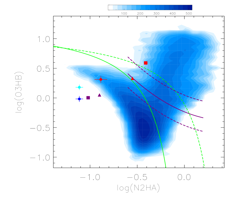
Based on the determined narrow emission line ratios by model A, the SDSS J1451+2709 is plotted in the BPT diagram of (flux ratio of [O iii] to narrow H) versus (flux ratio of [N ii] to narrow H) in Fig. 5. Considering the dividing lines in the BPT diagram as well discussed in Kauffmann et al. (2003); Kewley et al. (2006, 2019); Zhang et al. (2020), either [, ] or [, ] applied in the BPT diagram through the properties of narrow emission lines, the SDSS J1451+2709 can be well classified as a HII galaxy with few contributions of central AGN activities, against the physical properties of a normal blue quasar.
3.2 Flux ratios of narrow emission lines based on the model B
For the results by model B with broad Balmer lines described by Lorentz functions, the determined H and H have line widths quite larger than , therefore, the determined H and H can be safely accepted to be from central BLRs. However, the Lorentz described broad component H have the same line widths about 30Å () in the KPNO spectrum in 1990 and in the SDSS spectrum in 2007. Meanwhile, as the results shown in Fig. 3 and the parameters listed in Table 1, the continuum intensity at 5100Å and the broad H flux are brightened by 1.8 times from 1990 to 2007, indicating line width of broad H in the SDSS spectrum in 2007 should be about 1.16 times smaller than the one in the KPNO spectrum in 1990. However, the measured line width in 2007 is only 1.05times smaller than the value in 1990, indicating that the Lorentz described broad Balmer components include contributions of none-variability components (such as contributions from narrow Balmer emission lines from NLRs) or that the geometric structures of central BLRs are too extended.
Certainly, the forbidden narrow lines are considered and well accepted from the central NLRs. Then, comparing with the line width of extended component of [O iii]5007Å, the determined components of narrow emission lines with line widths smaller than can be safely accepted to be from central NLRs.
Finally, for the determined components shown in Fig. 3 and with parameters listed in the fifth column to the seventh column in Table 1, the broad components H, H are truly from central BLRs, the [N ii] doublet and the core and extended components of [O iii] doublet and narrow Balmer lines are from central NLRs. Therefore, flux ratio of [O iii]Å (both the core and the extended component) to narrow H (including two components, H and H) can be estimated as
| (5) |
Considering the model parameters of [N ii]Å and the core and extended components of narrow H listed in Table 1, the flux ratio of [N ii]Å to narrow H (including two components, H and H) can be estimated as
| (6) |
Based on the determined narrow emission line ratios by model B, the SDSS J1451+2709 can be re-plotted in the BPT diagram of versus in Fig. 5. The SDSS J1451+2709 can be well classified as a HII galaxy with few contributions of central AGN activities, through the properties of narrow emission lines.
Finally, based on different model functions to describe emission lines and based on different considerations of emission components from central NLRs, the SDSS J1451+2709 can be well classified as a HII galaxy with few contributions of central AGN activities. In the manuscript, the SDSS J1451+2709 can be called as a mis-classified quasar.
4 Physical origin of the mis-classified quasar SDSS J1451+2709?
In order to explain the mis-classified quasar SDSS J1451+2709, two reasonable methods are mainly considered in the section. On the one hand, there is one mechanism leading to stronger narrow Balmer emissions, such as the strong starforming contributions. On the other hand, there is one mechanism leading to weaker forbidden emission lines, such as the expected high electron densities in central NLRs.
4.1 Strong Starforming contributions?
In the subsection, we can check whether starforming contributions can be applied to explain the unique properties of SDSS J1451+2709 in the BPT diagram, because of stronger starforming contributions leading to stronger narrow Balmer emission lines. In other words, there are two kinds of flux components included in the narrow Balmer lines and [O iii]Å and [N ii]Å, one kind of flux depending on central AGN activities: , , and , the other kind of flux depending on starforming: , , and . Then, the measured flux ratio and , and the flux rations and depending on central AGN activities, and the flux ratios and depending on starforming, can be described as
| (7) |
where , , and mean the measured total line flux of [O iii]Å, [N ii]Å and narrow Balmer lines.
Based on the three measured data points shown in Fig. 5 and the corresponding measured total line fluxes , , and , expected properties of starforming contributions can be simply determined, through the following limitations. First, the determined flux ratios of and clearly lead the data points classified as AGN in the BPT diagram, the data points lying above the dividing line shown as solid green line in Fig. 5. Second, the determined flux ratios of and clearly lead the data points classified as AGN in the BPT diagram, the data points lying below the dividing line shown as solid green line in Fig. 5. Third, the ratios of to are similar as the ratios of to .
Based on the measured lime parameters by the model A with considering H from NLRs, the narrow emission line fluxes are abut , , and in the units of . Then, among 50000 randomly selected values of , of and of , there are 5000 couple data points of [, ] classified as AGN, and corresponding 5000 couple data points of [, ] classified as HII, in the BPT diagram of versus , shown in the left panel of Fig. 6. And top right panel of Fig. 6 shows the dependence of on , with the determined minimum value 71% of the .
Similarly, based on the measured lime parameters by the model A with considering H from BLRs, the narrow emission line fluxes are abut , , and in the units of . Then, among 40000 randomly selected values of , of and of , there are 5000 couple data points of [, ] classified as AGN, and corresponding 5000 couple data points of [, ] classified as HII, in the BPT diagram of versus . Here, we do not show the results in the BPT diagram, which are similar as the those shown in the left panel of Fig. 6 but with different positions of the data points. And the middle right panel of Fig. 6 shows the dependence of on , with the determined minimum value 63% of the .
Based on the measured lime parameters by the model B, the narrow emission line fluxes are abut , , and in the units of . Then, among 20000 randomly selected values of , of and of , there are 5000 couple data points of [, ] classified as AGN, and corresponding 5000 couple data points of [, ] classified as HII, in the BPT diagram of versus . Here, we do not show the results in the BPT diagram, which are similar as the those shown in the left panel of Fig. 6 but with different positions of the data points. And the bottom right panel of Fig. 6 shows the dependence of on , with the determined minimum value 42% of the .
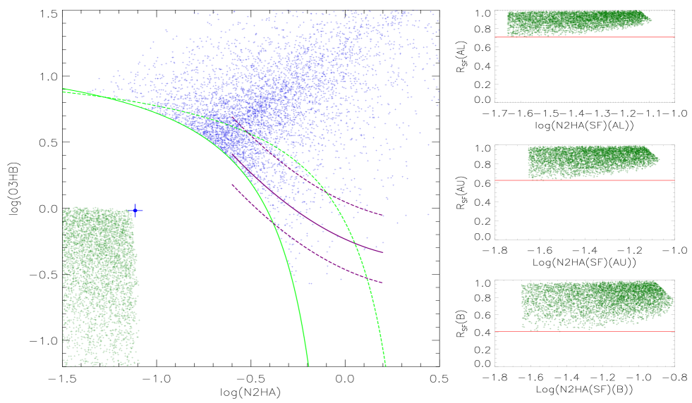
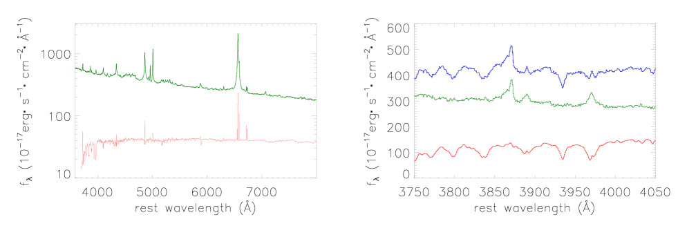
Therefore, by different model functions determined narrow line fluxes with different considerations, the determined starforming contributions should be larger than 40%, strongly indicating apparent absorption features from host galaxy in the spectrum of SDSS J1451+2709. Fig. 7 shows one composite spectrum created by 0.6 times of the SDSS spectrum of SDSS J1451+2709 plus a mean HII galaxy with continuum intensity at 5100Å about 0.4 times of the continuum intensity at 5100Å of the SDSS spectrum of SDSS J1451+2709. Here, the mean spectrum of HII galaxies are created by the large sample of 1298 HII galaxies with signal-to-noise larger than 30 in SDSS DR12. The absorption features are apparent enough in the composite spectrum with 40% starforming contributions. However, the clean quasar-like spectrum without clear absorption features, especially around 4000Å, clearly indicate that the starforming contributions cannot be applied to explain the unique properties of the mis-classified quasar SDSS J1451+2709 in the BPT diagram.
4.2 Compressed central NLRs?
Besides the starforming contributions, high electron density in NLRs can be also applied to explain the unique properties of the mis-classified quasar SDSS J1451+2709 in the BPT diagram, because the high electron density near to the critical electron densities of the forbidden emission lines can lead to suppressed line intensities of forbidden emission lines but positive effects on strengthened Balmer emission lines.
It is not hard to determine electron density in NLRs, such as through the flux ratios of [S ii]Å doublet as well discussed in Proxauf et al. (2014); Sanders et al. (2016); Kewley et al. (2019). Based on the measured line fluxes of [S ii] doublet listed in Table 1, the flux ratio of [S ii]Å to [S ii]Å lead the electron density to be estimated around , a quite normal value, quite smaller than the critical densities around to [O iii] and [N ii] doublet.
Based on the estimated electron density in NLRs, the compressed central NLRs with higher electron densities could not be preferred to explain the unique properties of the mis-classified quasar SDSS J1451+2709 in the BPT diagram. Certainly, the probability of the compressed central NLRs cannot be totally ruled out, considering different emission regions of [S ii] doublet from the emission regions of [O iii] and [N ii] doublet.
Unfortunately, neither the starforming contributions nor the compressed NLRs can be preferred in the mis-classified quasar SDSS J1451+2709. Further efforts are necessary to determine the physical origin of the unique properties of the mis-classified quasar SDSS J1451+2709 in the BPT diagram.
5 Long-term photometric variability properties
In the section, long-term variabilities of SDSS J1451+2709 are well checked, in order to check whether are there further clues on unique variability properties of the mis-classified quasar SDSS J1451+2709.
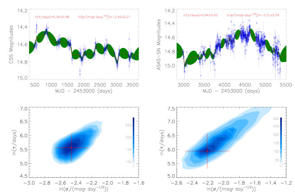
Besides the spectroscopic results for SDSS J1451+2709, long-term photometric variability can be collected from the Catalina Sky Survey (CSS, http://nesssi.cacr.caltech.edu/) (Drake et al., 2009; Larson et al., 2003) with with MJD from 2453470 to 2456567 shown in the top left panel in Fig. 8, and from the well-known All-Sky Automated Survey for Supernovae (ASAS-SN, https://asas-sn.osu.edu/) (Shappee et al., 2014; Kovacevic et al., 2017) with MJD from 2455978 to 2458737 shown in the top right panel in Fig. 8.
Now it is interesting to check the long-term variability of the mis-classified quasar SDSS J1451+2709 by the well-known Damped Random Walk process (DRW process or Continuous AutoRegressive process, CAR process) (Brockwell & Davis, 2002). The DRW process, with two basic parameters of the intrinsic variability timescale and the intrinsic variability amplitude , has been proved to be a preferred modeling process to describe AGN intrinsic variability. Kelly, Bechtold & Siemiginowska (2009) firstly proposed the CAR process to describe the AGN intrinsic variability, and found that the AGN intrinsic variability timescales are consistent with disk orbital or thermal timescales. Kozlowski et al. (2010) provided an improved robust mathematic method to estimate the DRW process parameters, and found that AGN variability could be well modeled by the DRW process. Then, Zu, Kochanek & Peterson (2011) provided a public code of JAVELIN (http://www.astronomy.ohio-state.edu/~yingzu/codes.html#javelin) (Just Another Vehicle for Estimating Lags In Nuclei) based on the method in Kozlowski et al. (2010) to describe the AGN variability by the DRW process.
Meanwhile, there are many other reported studies on the AGN variability through the DRW process. MacLeod et al. (2010) modeled the variability of about 9000 spectroscopically confirmed quasars covered in the SDSS Stripe82 region, and found correlations between the AGN parameters and the DRW process determined parameters. Bailer-Jones (2012) proposed an another fully probabilistic method for modeling AGN variability by the DRW process. Andrae, Kim & Bailer-Jones (2013) have shown that the DRW process is preferred to model AGN variability, rather than several other stochastic and deterministic models, by fitted results of long-term variability of 6304 quasars. Zu et al. (2013) have checked that the DRW process provided an adequate description of AGN optical variability across all timescales. More recently, in our previous paper, Zhang & Feng (2017a) have checked long-term variability properties of AGN with double-peaked broad emission lines, and found the difference in intrinsic variability timescales between normal broad line AGN and the AGN with double-peaked broad emission lines. Therefore, the DRW process determined parameters from the long-term AGN variability can be well used to check or predict further different properties of different kinds of AGN with probable different intrinsic properties of emission regions.
The public code of JAVELIN provided by Zu, Kochanek & Peterson (2011); Zu et al. (2013) has been applied here to describe the long-term variability shown in top panels of Fig. 8. When the JAVELIN code is applied, through the MCMC (Markov Chain Monte Carlo) analysis with the uniform logarithmic priors of the DRW process parameters of and covering every possible corner of the parameter space ( and ), the posterior distributions of the DRW process parameters can be well determined and shown in bottom panels of Fig. 8 and provide the final accepted parameters and the corresponding uncertainties. For the photometric CSS light curve, the determined DRW process parameters are and . For the photometric ASAS-SN light curve, the determined DRW process parameters are and . Although there are different time-steps and time durations of the CSS light curve and the ASAS-SN light curve, there are similar determined DRW process parameters of and , indicating the determined DRW process parameters are stable enough.
Comparing with variabilities of quasars discussed in Kelly, Bechtold & Siemiginowska (2009); MacLeod et al. (2010); Kozlowski et al. (2010), the mis-classified quasar SDSS J1451+2709 has the normal intrinsic variability timescale around 300days, however, have a large but also acceptable intrinsic variability amplitude around 0.1 (especially comparing with the results shown in Fig. 6 in Kozlowski et al. (2010)). It is clear that SDSS J1451+2709 has common long-term photometric variability properties.
6 Further implications of the mis-classified quasar SDSS J1451+2709
If the discussed results above are true for the mis-classified quasar SDSS J1451+2709, there are at least three further implications on the study of classifications by the BPT diagrams.
First and foremost, if the mis-classified quasar SDSS J1451+2709 was an extremely unique case among the quasars in the BPT diagram, there must be extremely special emission structures in SDSS J1451+2709, leading to quite lower flux ratios of narrow emission lines than normal quasars. The extremely unique case of the mis-classified quasar J1451+2709 deserves further study in the near future.
Besides, if the mis-classified quasar SDSS J1451+2709 was not an extremely unique case but a some special case among quasars in the BPT diagrams, there would be more mis-classified quasars which can be detected among normal quasars. To detect a sample of mis-classified quasars should provide clues that the mis-classified quasars should be a special subclass of type-1 AGN with some unknown special emission properties. Meanwhile, the results should indicate that there could be some narrow emission lines HII galaxies with probable central AGN activities.
Last but not the least, if the mis-classified quasar SDSS J1451+2709 was due to mis-applications of BPT diagrams to broad line AGN, it would be a challenge to the applications of BPT diagrams from narrow emission line objects to broad line AGN. Or, emission line fitting procedure determined emission line parameters are not so efficient for narrow emission lines?
7 Summaries and Conclusions
Finally, we give our main conclusions as follows.
-
•
Emission line parameters of the blue quasar SDSS J1451+2709 can be well measured by two different models, mode A with broad Gaussian functions applied to describe broad Balmer emission lines, and model B with broad Lorentz functions applied to described the broad Balmer emission lines.
-
•
Based on two-epoch spectra observed in SDSS in 2007 and observed by KPNO in 1990, broad Balmer emission components from central BLRs can be well determined. Besides the emission components from central BLRs, emission components from central NLRs can be estimated, leading to different flux ratios of narrow emission lines.
-
•
Different flux ratios of narrow emission lines determined by different model functions and with different considerations, the SDSS J1451+2709 can be well classified as a HII galaxy in the BPT diagram, although the SDSS J1451+2709 actually is a normal blue quasar.
-
•
Two reasonable methods are proposed to explain the unique properties of the mis-classified quasar SDSS J1451+2709 in the BPT diagram, strong starforming contributions leading to stronger narrow Balmer emissions, and compressed NLRs with high electron densities leading to suppressed forbidden emissions.
-
•
Once considering the starforming contributions, at least 40% starforming contributions should be preferred in the mis-classified quasar SDSS J1451+2709, which will lead to apparent absorption features around 4000Å. However, none apparent absorption features in the SDSS spectrum of the mis-classified quasar SDSS J1451+2709 indicate strong starforming contributions are not preferred in the mis-classified quasar SDSS J1451+2709.
-
•
Once considering the compressed NLRs with high electron densities, the expected electron densities should be around . However, the estimated electron density is only around based on the flux ratio of [S ii]Å to [S ii]Å. Therefore, the compressed NLRs with high electron densities are not preferred in the mis-classified quasar SDSS J1451+2709.
-
•
Further efforts are necessary to find reasonable physical origin of the unique properties of the mis-classified quasar SDSS J1451+2709 in the BPT diagram.
-
•
The long-term variability properties of the mis-classified quasar SDSS J1451+2709 are not quite different from the normal quasars.
-
•
The reported mis-classified quasar SDSS J1451+2709 strongly indicate that there should be extremely unique properties of SDSS J1451+2709 which are currently not detected, or indicate that there should be a small sample of mis-classified quasars similar as the SDSS J1451+2709, or indicate that there should be some narrow emission line HII galaxies intrinsically harbouring central AGN activities.
Acknowledgements
Zhang gratefully acknowledges the anonymous referee reading the manuscript with patience. Zhang gratefully acknowledges the kind support of Starting Research Fund of Nanjing Normal University, and gratefully acknowledges the kind support of NSFC-11973029. This manuscript has made use of the data from the SDSS projects. The SDSS-III web site is http://www.sdss3.org/. SDSS-III is managed by the Astrophysical Research Consortium for the Participating Institutions of the SDSS-III Collaborations. The manuscript has made use of the data from from the Catalina Sky Survey http://nesssi.cacr.caltech.edu/DataRelease/, and from the All-Sky Automated Survey for Supernovae https://asas-sn.osu.edu/. The manuscript has made use of the NASA/IPAC Extragalactic Database (NED) https://ned.ipac.caltech.edu/, which is funded by the National Aeronautics and Space Administration and operated by the California Institute of Technology.
Data Availability
The data underlying this article will be shared on reasonable request to the corresponding author (xgzhang@njnu.edu.cn).
References
- Antouncci (1993) Antonucci, R., 1993, ARA&A, 31, 473
- Audibert et al. (2017) Audibert, A., Riffel, R., Sales, D. A., Pastoriza, M. G., Ruschel-Dutra, D., 2017, MNRAS, 464, 2139
- Andrae, Kim & Bailer-Jones (2013) Andrae, R., Kim, D. W., & Bailer-Jones, C. A. L., 2013, A&A, 554, 137
- Bailer-Jones (2012) Bailer-Jones, C. A. L., 2012, A&A, 546, A89
- Balokovic et al. (2018) Balokovic, M.; Brightman, M. ; Harrison, F. A.; et al., 2018, ApJ, 854, 42
- Baldwin, Phillips & Terlevich (1981) Baldwin, J. A., Phillips, M., & Terlevich, R., 1981, PASP, 93, 5
- Bentz et al. (2006) Bentz, M. C., Peterson, B. M., Pogge, R. W., Vestergaard, M., Onken, C. A., 2006, ApJ, 644, 133
- Bentz et al. (2009) Bentz, M. C., Peterson, B. M., Netzer, H., Pogge, R. W., Vestergaard, M., 2009, ApJ, 697, 160
- Bentz et al. (2013) Bentz, M. C., et al., 2013, ApJ, 767, 149
- Boroson & Green (1992) Boroson, T. A.; Green, R. F., 1992, ApJS, 80, 109
- Brockwell & Davis (2002) Brockwell, P. J., & Davis, R. A. 2002, Introduction to Time Series and Forecasting (2nd ed.; New York: Springer)
- Brown et al. (2019) Brown, A.; Nayyeri, H.; Cooray, A.; Ma, J.; Hickox, R. C.; Azadi, M, 2019, ApJ, 871, 87
- Denney et al. (2010) Denney, K. D., et al., 2010, ApJ, 721, 715
- Drake et al. (2009) Drake, A. J., 2009, ApJ, 696, 870
- Fausnaugh et al. (2017) Fausnaugh, M. M., et al., 2017, ApJ, 840, 97
- Fischer et al. (2013) Fischer, T. C., Crenshaw, D. M., Kraemer, S. B., Schmitt, H. R., 2013, ApJS, 209, 1
- Fischer et al. (2017) Fischer, T. C., et al., 2017, ApJ, 834, 30
- Greene & Ho (2005) Greene, J. E., & Ho, L. C., 2005, ApJ, 627, 721
- Greene & Ho (2005b) Greene, J. E., & Ho, L. C., 2005b, ApJ, 630, 122
- Hainline et al. (2014) Hainline, K. N., et al., 2014, ApJ, 787, 65
- Heckman & Best (2014) Heckman, T. M.; Best, P. N., 2014, ARA&A, 52, 589
- Kauffmann et al. (2003) Kauffmann, G., et al. 2003, MNRAS, 346, 1055
- Kaspi et al. (2000) Kaspi, S., et al., 2000, ApJ, 533, 631
- Kaspi et al. (2005) Kaspi, S., et al., 2005, ApJ, 629, 61
- Kewley et al. (2001) Kewley, L. J., Dopita, M. A., Sutherland, R. S., Heisler, C. A., Trevena, J. 2001, ApJ, 556, 121
- Kewley et al. (2006) Kewley, L. J., Groves, B., Kauffmann, G., Heckman, T., 2006, MNRAS, 372, 961
- Kewley et al. (2006) Kewley, L. J., Groves, B.; Kauffmann, G.; Heckman, T., 2006, mnras, 372, 961
- Kewley et al. (2019) Kewley, L. J., Nicholls, D. C., Sutherland, R. S. 2019, ARA&A, 57, 511
- Kewley et al. (2019) Kewley, L. J.; Nicholls, D. C.; Sutherland, R.; et al., 2019, ApJ, 880, 16
- Kewley et al. (2013a) Kewley, L. J., et al., 2013a, ApJ, 774, 10
- Kewley et al. (2013b) Kewley, L. J., et al., 2013b, ApJ, 774, 100
- Kelly, Bechtold & Siemiginowska (2009) Kelly, B. C., Bechtold, J., & Siemiginowska, A., 2009, ApJ, 698, 895
- Kozlowski et al. (2010) Kozlowski, S., et al., 2010, ApJ, 708, 927
- Kovacevic et al. (2010) Kovacevic, J., Popovic, L. C., Dimitrijevic, M. S., 2010, ApJS, 189, 15
- Kovacevic et al. (2017) Kochanek, C. S.; Shappee, B. J.; Stanek, K. Z.; etal., 2017, PASP, 129, 4502
- Kuraszkiewicz et al. (2021) Kuraszkiewicz, J.; Wilkes, B. J.; Atanas, A.; et al., 2021, ApJ, 913, 134
- Larson et al. (2003) Larson, S., et al., 2003, DPS, 35, 3604
- Lyke et al. (2020) Lyke, B. W.; Higley, A. N. ; McLane, J. N.; et al., 2020, ApJS, 250, 8
- MacLeod et al. (2010) MacLeod C. L., et al., 2010, ApJ, 721, 1014
- Netzer (2015) Netzer, H., 2015, ARA&A, 53, 365
- Peterson et al. (2004) Peterson, B. M., et al., 2004, ApJ, 613, 682
- Peters et al. (2015) Peters, C. M.; Richards, G. T.; Myers, A. D.; et al., 2015, ApJ, 811, 95
- Proxauf et al. (2014) Proxauf, B.; Ottl, S.; Kimeswenger, S., 2014, A&A, 561, 10
- Rafiee & Hall (2011) Rafiee, A., & Hall, P. B., 2011, ApJS, 194, 42
- Ramos et al. (2011) Ramos, A. C., et al., 2011, ApJ, 731, 92
- Richards et al. (2002) Richards, G. T., et al., 2002, AJ, 123, 2945
- Ross et al. (2012) Ross, N. P., et al., 2012, ApJS, 199, 3
- Sanders et al. (2016) Sanders, R. L., Shapley, A. E., Kriek, M., et al. 2016, ApJ, 816, 23
- Shappee et al. (2014) Shappee, B. J.; Prieto, J. L.; Grupe, D.; et al., 2014, ApJ, 788, 48
- Shen et al. (2011) Shen, Y., et al., 2011, ApJS, 194, 45
- Sun et al. (2017) Sun, A. L.; Greene, J. E.; Zakamska, N. L., 2017, ApJ, 835, 222
- Vestergaard (2002) Vestergaard, M., 2002, ApJ, 571, 733
- Vestergaard & Peterson (2006) Vestergaard, M., & Peterson, B. M., 2006, ApJ, 641, 689
- Zakamska et al. (2003) Zakamska, N. L., et al., 2003, AJ, 126, 2125
- Zhang & Feng (2016) Zhang, X. G., & Feng, L. L., 2016, MNRAS, 457, 3878
- Zhang & Feng (2017a) Zhang, X. G., & Feng, L. L., 2017a, MNRAS, 464, 2203
- Zhang & Feng (2017) Zhang, X. G., & Feng, L. L., 2017, MNRAS, 468, 620
- Zhang et al. (2020) Zhang, X. G., Feng Y., Chen, H., Yuan, Q., 2020, ApJ, 905, 97
- Zhang (2021a) Zhang, X. G., 2021a, ApJ, 909, 16
- Zhang (2021b) Zhang, X. G., 2021b, MNRAS, 502, 2508
- Zu, Kochanek & Peterson (2011) Zu, Y., Kochanek, C. S., & Peterson, B. M., 2011, ApJ, 735, 80
- Zu et al. (2013) Zu, Y., Kochanek, C. S., Kozlowski, S., Udalski, A., 2013, ApJ, 765, 106