Finite-Time Dynamical Phase Transition in Non-Equilibrium Relaxation

Abstract

We uncover a finite-time dynamical phase transition in the thermal relaxation of a mean-field magnetic model. The phase transition manifests itself as a cusp singularity in the probability distribution of the magnetisation that forms at a critical time. The transition is due to a sudden switch in the dynamics, characterised by a dynamical order parameter. We derive a dynamical Landau theory for the transition that applies to a range of systems with scalar, parity-invariant order parameters. Close to criticalilty, our theory reveals an exact mapping between the dynamical and equilibrium phase transitions of the magnetic model, and implies critical exponents of mean-field type. We argue that interactions between nearby saddle points, neglected at the mean-field level, may lead to critical, spatiotemporal fluctuations of the order parameter, and thus give rise to novel, dynamical critical phenomena.

The dynamic response of many-body systems to changes of the external parameters, be it the temperature, pressure or an external field, is of fundamental interest in statistical mechanics and has a wide range of applications. When the changes are small, the response of the system is linear [1, 2, 3, 4], and rather well understood [5, 6, 7]. In many applications, however, the external parameters switch suddenly and violently, thus driving the system far away from equilibrium. Non-equilibrium relaxation phenomena are theoretically [8, 9, 10] and experimentally [11, 12, 13] challenging, in particular when they exhibit long transients [14, 15], which is often the case in the presence of phase transitions.

Equilibrium phase transitions are qualitative changes of a system’s equilibrium state under adiabatic variation of the external parameters [16]. They are accompanied by characteristic changes of order parameters [17], such as the density or the magnetisation. At continuous phase transitions, thermodynamic quantities and order parameters exhibit power-law behaviour [18], and the values of their critical exponents divide systems into universality classes. Recent developments [19, 20, 21, 22, 23, 24] have given rise to conceptual generalisations of phase transitions to non-equilibrium systems [25, 26, 27, 28, 29, 30] and dynamic observables [31, 32, 33, 34, 35, 36, 37, 38]. These “dynamical phase transitions” are related to qualitative changes in the dynamics [39, 40, 41, 42, 43], observed in the long-time limit, under varying external conditions.

In this Letter, we uncover a finite-time dynamical phase transition in the non-equilibrium relaxation of a classical, mean-field spin model. In distinction to other classical transitions, the present one occurs in the transient response to an instantaneous change (a “quench”) of the temperature that induces an order-to-disorder phase transition. Interestingly, dynamical phase transitions with similar properties have recently been found in closed quantum systems [44, 45]. The transition manifests itself as a transient cusp singularity in the probability distribution of the magnetisation and is the result of competing dynamic behaviours within the system. The interpretation of this cusp as a phase transition sheds new light on previous works [46, 47, 48, 49, 50, 51] that discuss mathematical details of the singularity, and the existence and absence of a Gibbs measure for the transient. We derive a dynamical Landau theory for the phase transition that is robust against symmetry preserving transformations, and which applies to a range of systems with scalar, parity-invariant order parameters. An exact mapping between the dynamical and equilibrium phase transitions of the magnetic model classifies the transition as continuous, with mean-field-type critical exponents.

The Curie-Weiss model consists of $N\to\infty$ coupled Ising spins $\sigma_{i}=\pm 1$, $i=1,\ldots,N$, with infinite-range, ferromagnetic interaction of strength $J/(2N)$. The system is immersed in a heat bath at inverse temperature $\beta=1/(k_{\text{B}}T)$, and subject to an external field $H$. Because of the mean-field nature of the interaction, all states with equal numbers $N_{\pm}$ of spins in the states $\pm 1$, respectively, are equivalent. Therefore, any microstate can be written in terms of the total magnetisation $M=N_{+}-N_{-}$. The free energy $F$ reads [17]

$$F(M)=-\frac{J}{2N}\left(M^{2}-N\right)-MH-\beta^{-1}S(M)\,,$$ (1)

where the dimensionless internal entropy $S(M)=\ln\Omega(M)$ originates from the microscopic degeneracy $\Omega(M)$ of $M$.

We endow the system with a stochastic dynamics mediated by thermal fluctuations of the heat bath. A transition $\mp 1\to\pm 1$ of an arbitrary spin leads to $M\to M_{\pm}\equiv M\pm 2$. The evolution of the probability $P(M,t)$ for finding the system in state $M$ at time $t$ is described by the master equation

$$\dot{P}(M,t)=\sum_{\eta=\pm}\left[W_{\eta}(M_{-\eta})P(M_{-\eta},t)-W_{\eta}(M)P(M,t)\right]\,,$$ (2)

where $W_{\pm}(M)$ are the rates for $M\to M_{\pm}$, given by

$$W_{\pm}(M)=\frac{N\mp M}{2\tau}\exp\left\{\pm\beta\left[\frac{J}{N}\left(M\pm 1\right)+H\right]\right\}\,,$$ (3)

with microscopic relaxation time $\tau$. The algebraic prefactor $\propto(N\mp M)/2=N_{\mp}$ is due to equivalence of microscopic transitions, and spin-inversion invariance implies parity symmetry in $M$, $W_{\pm}(M)|_{H=0}=W_{\mp}(-M)|_{H=0}$. Forward and backward rates are related by detailed balance [52], $W_{\pm}(M)P^{\text{eq}}(M)=W_{\mp}(M_{\pm})P^{\text{eq}}(M_{\pm})$, with respect to the equilibrium distribution $P^{\text{eq}}(M)=Z^{-1}\exp\left[-\beta F(M)\right]$; $Z$ denotes the partition function.

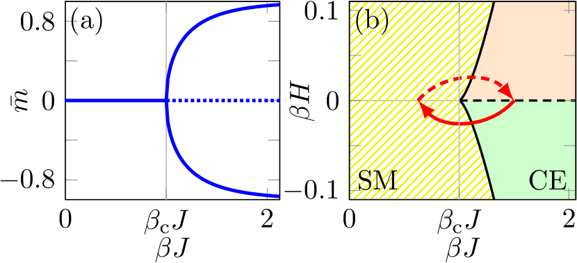
Figure 1: (a) Magnetisation $\bar{m}$ at $H=0$. Solid lines show minima of $\mathscr{V}^{\text{eq}}$, the dotted line a local maximum. (b) Equilibrium phase diagram, featuring the SM phase (lined) and CE phase (filled), separated by the phase boundary (solid black line). At the dashed line, $\bar{m}$ jumps discontinuously. Red arrows indicate disordering (solid line) and ordering (dashed line) quenches, respectively.

To take the thermodynamic limit, $N\to\infty$, we define the intensive magnetisation $m\equiv M/N$ per spin and the free-energy density $\mathscr{F}(m)\equiv F(Nm)/N$. The equilibrium distribution for $m$ then takes the large-deviation form $P^{\text{eq}}(m)\smilefrown\exp\left[-N\mathscr{V}^{\text{eq}}(m)\right]$ [21, 53] with equilibrium rate function $\mathscr{V}^{\text{eq}}(m)=\beta\left[\mathscr{F}(m)-\mathscr{F}(\bar{m})\right]$, where $\mathscr{F}(m)=-Jm^{2}/2-mH-\beta^{-1}\mathscr{S}(m)$ and $\mathscr{S}(m)=-(1/2)\sum_{\eta=\pm}\left(1+\eta m\right)\ln\left(1+\eta m\right)+\ln 2$. The term $\mathscr{F}(\bar{m})=\min_{m}\mathscr{F}(m)$ originates from the normalisation of $P^{\text{eq}}(M)$ and $\bar{m}$ denotes the order parameter, the mean magnetisation $\bar{m}\approx\langle m\rangle$ in the thermodynamic limit. Expanding $\mathscr{V}^{\text{eq}}(m)$ to quartic order in $m$, one finds

$$\mathscr{V}^{\text{eq}}(m)\sim-\beta Hm-J\left(\beta-\beta_{\text{c}}\right)\frac{m^{2}}{2}+\frac{m^{4}}{12}-\beta\mathscr{F}(\bar{m})\,,$$ (4)

where the quadratic term changes sign at $\beta_{\text{c}}=1/J$ while the quartic term remains positive. Hence, for $H=0$, $\mathscr{V}^{\text{eq}}(m)$ passes from a single well to a symmetric double well at the critical inverse temperature $\beta_{\text{c}}$. This corresponds to a continuous phase transition [54] from a disordered into an ordered state, that spontaneously breaks the parity symmetry in $m$.

Close to $\beta_{\text{c}}$, $\bar{m}$ changes continuously from $\bar{m}=0$ to finite $\bar{m}$, as shown in Fig. 1(a). Figure 1(b) shows the phase diagram of the model, exhibiting two distinct phases, separated by a phase boundary (solid black line): a single-mode (SM) phase, where $\mathscr{V}^{\text{eq}}$ has a unique minimum, and a coexistence (CE) phase, where local and global minima coexist. Within the CE phase, $H\neq 0$ lifts the degeneracy between the two minima in $\mathscr{V}^{\text{eq}}(m)$, and thus splits the CE phase into regions with $\bar{m}>0$ (orange) and $\bar{m}<0$ (green). Moving across the dashed line that separates the two, $\bar{m}$ jumps discontinuously to $-\bar{m}$.

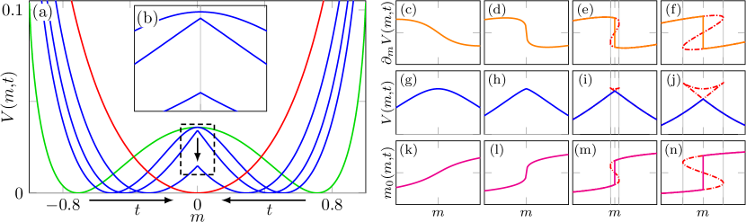
Figure 2: Post-quench dynamics for $\beta=5/(4J)$ and $\beta_{\text{q}}=3/(4J)$. (a) Rate functions $\mathscr{V}^{\text{eq}}$ (green), $\mathscr{V}^{\text{eq}}_{q}$ (red), and $V(m,t)$ for $t/\tau=0.5$, $0.8$ and $1.5$ (blue). Black arrows indicate the time evolution of $V(m,t)$. (b) Magnification of the dashed rectangle in Fig. 2(a). (c)–(n) Time evolution of $\partial_{m}V(m,t)$ [(c)–(f)], $V(m,t)$ [(g)–(j)] and $m_{0}(m,t)$ [(k)–(n)] for $t/\tau=0.5$, $0.7$, $0.8$, and $1$ (from left to right). The solid and dash-dotted lines show dominant and sub-dominant solutions, respectively (see main text). Gray lines delimit the dynamical coexistence region.

In the vicinity of the critical point, $(\beta,H)=(\beta_{\text{c}},0)$, we obtain from the minimisation condition $\text{d}\mathscr{V}^{\text{eq}}/\text{d}m|_{m=\bar{m}}=0$, an equation of state that leads to mean-field critical exponents [18, 17], universal among mean-field models. In particular, for $H=0$ one finds that $\bar{m}(\beta)$ is continuous, with $\bar{m}=0$ and $\bar{m}\propto|\beta-\beta_{\text{c}}|^{1/2}$, below and slightly above $\beta_{\text{c}}$, respectively.

Starting from an ordered equilibrium state in the CE phase with $\beta>\beta_{\text{c}}$ at time $t<0$, we induce an instantaneous disordering quench $\beta\to\beta_{\text{q}}$ into the SM phase, $\beta_{\text{q}}<\beta_{\text{c}}$, at $t=0$. For simplicity, we set $H=0$. Because the quench crosses the phase boundary [solid arrow in Fig. 1(b)], it induces an order-to-disorder phase transition. In contrast to ordering quenches [dashed arrow in Fig. 1(b)] [14], disordering quenches are ergodic, so that $P(m,t)\to P^{\text{eq}}_{q}(m)\smilefrown\exp[-N\mathscr{V}^{\text{eq}}_{q}(m)]$ as $t\to\infty$, where $\mathscr{V}^{\text{eq}}_{q}(m)$ is the equilibrium rate function at the final inverse temperature $\beta_{\text{q}}$.

For $t>0$, the post-quench dynamics of the probability distribution $P(m,t)\smilefrown\exp[-NV(m,t)]$, with time-dependent rate function $V(m,t)$, is determined by Eq. (2) which turns into the Hamilton-Jacobi equation

$$0=\partial_{t}V(m,t)+\mathscr{H}[m,\partial_{m}V(m,t)]\,,$$ (5)

to leading order in $N\gg 1$, with initial condition $V(m,0)=\mathscr{V}^{\text{eq}}(m)$ and Hamiltonian [55, 56, 57]

$$\mathscr{H}(q,p) =w_{+}(q)\left(\text{e}^{2p}-1\right)+w_{-}(q)\left(\text{e}^{-2p}-1\right)\,;$$ (6)

see Sec. I in the Supplemental Material [58]. Here, $w_{\pm}(q)=(2\tau)^{-1}(1\mp q)\exp\left(\pm\beta_{\text{q}}Jq\right)$ denote the $N$-scaled transition rates. Solutions to Eq. (5) are given in terms of characteristics $q(s)$ and $p(s)$, $0\leq s\leq t$, that solve the Hamilton equations [59]

$$\dot{q}(s)=\partial_{p}\mathscr{H}(q,p)\,,\quad\dot{p}(s)=-\partial_{q}\mathscr{H}(q,p)\,,$$ (7)

with boundary conditions

$$p(0)=\tfrac{\text{d}}{\text{d}m}\mathscr{V}^{\text{eq}}[q(0)]\,,\qquad q(t)=m\,.$$ (8)

From the solutions of Eqs. (7)–(8), $V(m,t)$ is obtained as

$$V(m,t)=\int_{0}^{t}\text{d}s\left[p\dot{q}-\mathscr{H}(q,p)\right]+\mathscr{V}^{\text{eq}}[q(0)]\,.$$ (9)

Any solution of Eqs. (7) and (8) solves the variational problem $\delta V(m,t)=0$, where $\delta$ denotes a variation over all trajectories with final point $q(t)=m$ [60, 59], i.e., all characteristics $[q(s),p(s)]_{0\leq s\leq t}$ are saddle points of Eq. (9). From the large-deviation form $P(m,t)\smilefrown\exp[-NV(m,t)]$ we conclude that only those characteristics that minimise $V(m,t)$ contribute for $N\to\infty$, and the others are exponentially suppressed. The minimising characteristic $q(s)$, $0\leq s\leq t$, constitutes the system’s optimal fluctuation, the most likely way to realise the magnetisation $q(t)=m=\lim_{N\to\infty}M(t)/N$ at time $t$, in response to the quench at $t=0$. In particular, $m_{0}(m,t)\equiv q(0)$ corresponds to the most likely initial magnetisation, which plays the role of an order parameter, as we explain below.

We compute $V(m,t)$ by solving Eqs. (7)–(8) with a shooting method [61] on a fine $m$ grid, see Sec. II in the Supplemental Material. We extract three fields: $V(m,t)$ [by evaluating Eq. (9)], the derivative field $\partial_{m}V(m,t)=p(t)$ [the end point of $p(s)$], and the initial magnetisation $m_{0}(m,t)=q(0)$.

The blue curves in Fig. 2(a) show $V(m,t)$ for different $t$; the green and red curves show $\mathscr{V}^{\text{eq}}$ and $\mathscr{V}^{\text{eq}}_{q}$, respectively. For small times, $V(m,t)$ is a symmetric double well, similar to the initial $\mathscr{V}^{\text{eq}}$. As $t$ increases, the minima of $V(m,t)$ move towards the origin, and the local maximum at $m=0$ decreases, as indicated by the black arrows in Fig. 2(a). In the long-time limit, $V(m,t)$ approaches the single-mode shape of $\mathscr{V}^{\text{eq}}_{q}$.

Notably, however, $V(m,t)$ does not evolve smoothly: At a finite time $t$, $V(m,t)$ forms a cusp at $m=0$ [see Fig. 2(b)], and the derivative field $\partial_{m}V(m,t)$ develops a discontinuous jump. The origin of this jump is shown in Figs. 2(c)–2(f): As time evolves, $\partial_{m}V(m,t)$ folds over and becomes multi-valued, and up to three solutions of Eqs. (7) and (8) coexist within a finite interval, delimited by the gray lines in Figs. 2(e) and 2(f). Selecting the one with smallest $V(m,t)$ naturally leads to a Maxwell construction for the dominant solution, shown in orange. The sub-dominant solutions [red, dash-dotted lines in Fig. 2(c)–2(f)] have a larger $V(m,t)$ as shown in Figs. 2(g)–(j). Figures 2(k)–2(n) indicate the same multivaluedness, and an analogous Maxwell construction for $m_{0}(m,t)$, culminating in a discontinuous jump at $m=0$.

Interpreting the formation of the cusp as a finite-time dynamical phase transition, we exploit the similarities with the equilibrium transition of the model. We first note that the sudden change of $m_{0}(m,t)$ at $m=0$ is strikingly similar to the discontinuous jump of $\bar{m}$ at equilibrium, when the external field $H$ crosses zero in the CE phase [dashed line in Fig. 1(b)]. To be specific, we identify $t$, $m_{0}$, and $m$ in the dynamical case with $\beta$, $\bar{m}$, and $H$, respectively, at equilibrium, and draw a “dynamical phase diagram”, shown in Fig. 3(a): Small times $t<t_{\text{c}}$ correspond to the dynamical single-mode (DSM) phase (yellow, lined region) where the dynamical order parameter $m_{0}(m,t)$ is unique (just like $\bar{m}$ for $\beta<\beta_{\text{c}}$) and $V(m,t)$ is a smooth function of $m$. For $t>t_{\text{c}}$ the system transitions into a dynamical coexistence (DCE) phase (filled region) where multiple $m_{0}$ values coexist. The DCE phase corresponds to the $m$ interval delimited by the gray lines in Figs. 2(m) and 2(n). For $m=0$, the two values, $m_{0}$ and $-m_{0}$ are degenerate, and parity symmetry is spontaneously broken by the dynamics, in analogy with $\bar{m}$ and $-\bar{m}$ for $\beta>\beta_{\text{c}}$ and $H=0$. Conditioning on $m\neq 0$ lifts this degeneracy, so that one of the $m_{0}$ values becomes exponentially suppressed. Consequently, when crossing the dashed line in the DCE phase in Fig. 3(a), $m_{0}$ jumps discontinuously, leading to the kink in $V(m,t)$ at $m=0$.

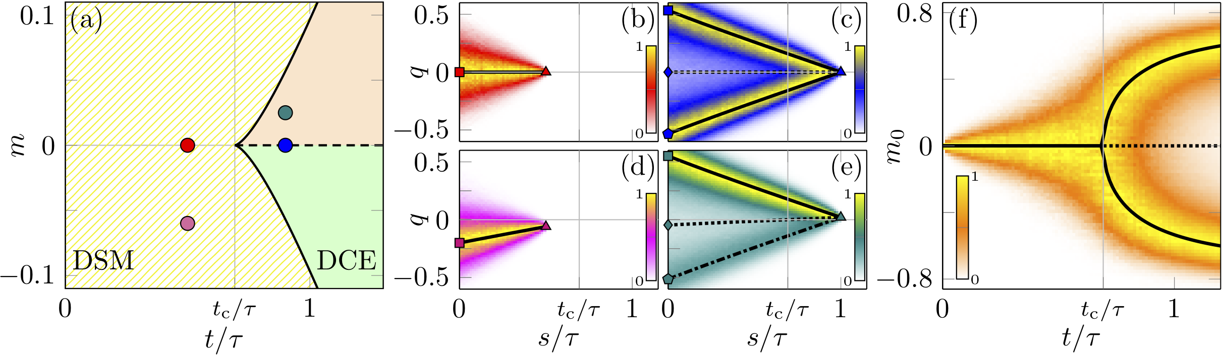
Figure 3: (a) Dynamical phase diagram for $(\beta,\beta_{\text{q}})=[5/(4J),3/(4J)]$, featuring the DSM (yellow, lined) and DCE (filled) phases (see main text), separated by a phase boundary (solid black line). The DCE phase splits into regions with $m_{0}(m,t)>0$ (orange) and $m_{0}(m,t)<0$ (green). At the dashed line, $m_{0}(m,t)$ jumps discontinuously. The bullets show $(t,m)$ values of the equally coloured trajectory densities in Fig. 3(b)–3(e). (b)–(e) Optimal fluctuations from theory (solid black line) and from numerical simulations (coloured regions, $N=200$, $10^{8}$ trajectories). Sub-dominant trajectories are shown as broken lines, symbols mark $m_{0}(m,t)=q(0)$ and $m=q(t)$. (f) Density of $m_{0}$ at $m=0$ as function of $t$ from numerical simulations (coloured region, $N=200$, $10^{8}$ trajectories), and optimal (solid black line) and sub-dominant (dotted line) $m_{0}(0,t)$ from theory.

On the trajectory level, the transition from the DSM into the DCE phase corresponds to a sudden change of the optimal fluctuation that minimises $V(m,t)$ in Eq. (9) [48, 49]. This follows from the dynamical analogue of an energy-entropy argument [18]: For small times, the right-hand side of Eq. (9) is dominated by the first term, interpreted as an activity. For $m=0$, this term is minimised by the inactive solution $p(s)=q(s)=0$, but at the cost of an unfavourable initial $q(0)=0$, the local maximum of the static, second term $\mathscr{V}^{\text{eq}}$. For long times, the activity term loses its dominance and $\mathscr{V}^{\text{eq}}$ becomes important so that the optimal fluctuation optimises $q(0)$ by starting at the minima of $\mathscr{V}^{\text{eq}}$.

To visualise the optimal fluctuations, we perform numerical simulations at finite $N$. From Eq. (2), we generate a large number of trajectories and record $q(s)\approx M(s)/N$, for different $0\leq s\leq t$, conditioning them to end up at $q(t)\in[m-\text{d}m,m+\text{d}m]$ for given $t$ and $m$, and a small $\text{d}m$. We then collect histograms of $q(s)$, normalised to unity for each $s$, and merge them, to obtain a numerical approximation of the trajectory density, shown in Figs. 3(b)–3(e). The colour coding matches their $(t,m)$ values, shown as the equally-coloured bullets in Fig. 3(a).

Figures 3(b) and 3(c) show good agreement between the optimal fluctuations (solid black line) and the yellow regions of high trajectory density in the DSM and DCE phase, respectively, at $m=0$. In the DSM phase [Fig. 3(b)], we observe a unique optimal fluctuation that remains at zero, the inactive solution. Beyond the dynamical critical point [Fig. 3(c)], two degenerate optimal fluctuations coexist, with initial magnetisations $m_{0}$ and $-m_{0}$ close to the minima of $\mathscr{V}^{\text{eq}}$. The third trajectory (dotted line) has a larger $V(m,t)$, and is not observed in the numerics.

Figures 3(d) and 3(e) show the optimal fluctuations and trajectory densities for finite $m$. In the DSM phase [Fig. 3(d)], the conditioning shifts the optimal fluctuation away from zero. Finite $m$ in the DCE phase [Fig. 3(e)] lifts the degeneracy between the optimal fluctuations, so that one of them is degraded to a local minimum of $V(m,t)$ (dash-dotted line), whose remnants persist at finite $N$.

In Fig. 3(f) we visualise the dependence of the order parameter $m_{0}(m,t)$ on $t$ by joining the histograms of $m_{0}=q(0)\approx M(0)/N$ for $m=0$ and different $t$. The solid black line shows the theoretical prediction for $m_{0}(0,t)$, obtained from Eqs. (7)–(8). Apart from the excellent agreement between the yellow regions and the theoretical curves, we observe a close similarity with the dependence of $\bar{m}$ on $\beta$, see Fig. 1(a).

To classify the dynamical phase transition in terms of equilibrium categories, we express $V(m,t)$ as the minimum of a dynamical Landau potential $\mathscr{L}^{m,t}(m_{0})$, $V(m,t)=\min_{m_{0}}\mathscr{L}^{m,t}(m_{0})-\beta\mathscr{F}(\bar{m})$, with the minimiser given by the dynamical order parameter $m_{0}(m,t)$. We then show that this provides an exact mapping between the dynamical phase diagram and the equilibrium one, close to the critical point.

First, we calculate the critical time $t_{\text{c}}$ for the transition. Since $V(0,t)$ develops a kink at time $t=t_{\text{c}}$, the curvature $z(t)\equiv\partial_{m}^{2}V(0,t)$ must tend to negative infinity, $z(t)\to-\infty$ as $t\to t_{\text{c}}$. Taking a partial derivative of Eq. (7), we find that $z(t)$ obeys a Riccati equation whose solution tends to $-\infty$ at $t_{\text{c}}/\tau=\ln\left[(\beta-\beta_{\text{q}})/(\beta-\beta_{\text{c}})\right]/[4(\beta_{\text{c}}-\beta_{\text{q}})J]$, see Sec. III in the Supplemental Material for details, and Ref. [49] for a different method. With the parameters of Figs. 2 and 3, we obtain $t_{\text{c}}/\tau=\ln(2)\approx 0.6931$, in agreement with the numerical result.

We now derive the Landau potential $\mathscr{L}^{m,t}(m_{0})$, whose minimum is attained by $m_{0}(m,t)$, analogous to the minimum $\bar{m}$ of $\mathscr{V}^{\text{eq}}$ at equilibrium. Close to the critical point, we expand $\mathscr{H}$ perturbatively to fourth order in $q$ and $p$, $\mathscr{H}\sim\mathscr{H}_{0}+\mathscr{H}_{1}$. A sequence of canonical transformations brings the quadratic and quartic Hamiltonians $\mathscr{H}_{0}$ and $\mathscr{H}_{1}$ into the forms $\mathscr{H}_{0}=(p^{2}-q^{2})/2$ and $\mathscr{H}_{1}=\alpha(p^{4}+q^{4})/4$, with real parameter $\alpha(\beta,\beta_{\text{q}},J)$. Using Eq. (9), we then compute $\mathscr{L}^{m,t}(m_{0})$ perturbatively to fourth order in $m_{0}$ and lowest order in $m$, see Sec. IV in the Supplemental Material. We find

$$\mathscr{L}^{m,t}(m_{0})\sim-m\lambda_{0}m_{0}-\lambda_{1}\left(\frac{t-t_{\text{c}}}{\tau}\right)\frac{m_{0}^{2}}{4}+\left[\lambda_{2}+\ldots\right]\frac{m_{0}^{4}}{4}\,,$$ (10)

where $\lambda_{0,1}>0$ and $\lambda_{2}>0$ for $\beta<3/(2J)$, and arbitrary $\beta_{\text{q}}$ and $J$; the dots denote higher-order terms in $t-t_{\text{c}}$. For $m=0$, $\mathscr{L}^{m,t}(m_{0})$ transitions from a single into a double well at the critical time $t_{\text{c}}$, just like $\mathscr{V}^{\text{eq}}$ at $\beta_{\text{c}}$. In other words, Eq. (10) is the dynamical analogue of Eq. (4) and both expressions can be mapped onto each other by proper rescaling of, e.g., $t-t_{\text{c}}$, $m_{0}$, and $m$. Hence, the dynamical phase transition has mean-field critical exponents and $m_{0}$ changes continuously from $m_{0}=0$ to $m_{0}\propto|t-t_{\text{c}}|^{1/2}$, below and above $t_{\text{c}}$, respectively. By contrast, for $\beta>3/(2J)$ we can have $\lambda_{2}<0$, and the system may undergo a discontinuous, first-order dynamical phase transition, where $m_{0}(m,t)$ jumps discontinuously. Symmetry-preserving transformations of the rates $W_{\pm}(M)\to\tilde{W}_{\pm}(M)$ leave $\lambda_{0,1}$ invariant, suggesting that the occurrence of the transition is model independent (Sec. V in the Supplemental Material).

Our dynamical Landau theory applies to an entire class of systems with scalar, parity-symmetric order parameters. A particularly simple one, that could be realised in a state-of-the-art experiment [62, 63], is a Brownian particle at weak noise, subject to a potential quench from a double into a single well (Sec. IV.B in the Supplemental Material).

Close to the critical point, interactions between nearby saddles $\delta V(m,t)=0$ of Eq. (9), neglected here, may lead to critical, spatiotemporal fluctuations of the order parameter, analogous to equilibrium [18, 17], and give rise to corrections to the mean-field exponents. The presence of strong fluctuations is indicated by the divergence $\propto|t-t_{\text{c}}|^{-1/2}$ of the pre-exponential factor of $P(m,t)$ at the critical point, see Sec. VI in the Supplemental Material. Since these fluctuations are of dynamical origin, we hypothesise that their effects are different from the equilibrium ones, and thus reflect a novel, dynamical critical phenomenon. This can be tested by investigating the post-quench dynamics of systems with short-range interactions in two and three dimensions using Monte-Carlo simulations [64], or perhaps dynamic renormalisation group methods [65].