FastFlow: Unsupervised Anomaly Detection and Localization
via 2D Normalizing Flows

Abstract

Unsupervised anomaly detection and localization is crucial to the practical application when collecting and labeling sufficient anomaly data is infeasible. Most existing representation-based approaches extract normal image features with a deep convolutional neural network and characterize the corresponding distribution through non-parametric distribution estimation methods. The anomaly score is calculated by measuring the distance between the feature of the test image and the estimated distribution. However, current methods can not effectively map image features to a tractable base distribution and ignore the relationship between local and global features which are important to identify anomalies. To this end, we propose FastFlow implemented with 2D normalizing flows and use it as the probability distribution estimator. Our FastFlow can be used as a plug-in module with arbitrary deep feature extractors such as ResNet and vision transformer for unsupervised anomaly detection and localization. In training phase, FastFlow learns to transform the input visual feature into a tractable distribution and obtains the likelihood to recognize anomalies in inference phase. Extensive experimental results on the MVTec AD dataset show that FastFlow surpasses previous state-of-the-art methods in terms of accuracy and inference efficiency with various backbone networks. Our approach achieves 99.4% AUC in anomaly detection with high inference efficiency.

1 Introduction

The purpose of anomaly detection and localization in computer vision field is to identify abnormal images and locate abnormal areas, which is widely used in industrial defect detection (Bergmann et al. 2019, 2020), medical image inspection (Philipp Seeböck et al. 2017), security check (Akcay, Atapour-Abarghouei, and Breckon 2018) and other fields. However, due to the low probability density of anomalies, the normal and abnormal data usually show a serious long-tail distribution, and even in some cases, no abnormal samples are available. The drawback of this reality makes it difficult to collect and annotate a large amount of abnormal data for supervised learning in practice. Unsupervised anomaly detection has been proposed to address this problem, which is also denoted as one-class classification or out-of-distribution detection. That is, we can only use normal samples during training process but need to identify and locate anomalies in testing.

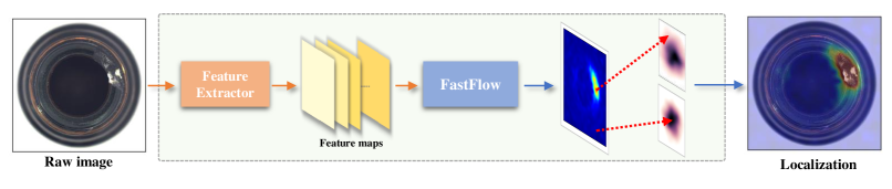
Figure 1: An example of the proposed FastFlow. FastFlow transforms features of the input image from the original distribution to the standard normal distribution. The features of the normal area in the input image fall in the center of the distribution, while the abnormal features are far away from the center of the distribution.

One promising method in unsupervised anomaly detection is using deep neural networks to obtain the features of normal images and model the distribution with some statistical methods, then detect the abnormal samples that have different distributions (Bergman and Hoshen 2020; Rippel, Mertens, and Merhof 2021; Yi and Yoon 2020; Cohen and Hoshen 2020; Defard et al. 2020). Following this methodology, there are two main components: the feature extraction module and the distribution estimation module.

To the distribution estimation module, previous approaches used the non-parametric method to model the distribution of features for normal images. For example, they estimated the multidimensional Gaussian distribution (Li et al. 2021; Defard et al. 2020) by calculating the mean and variance for features, or used a clustering algorithm to estimate these normal features by normal clustering (Reiss et al. 2021; Roth et al. 2021). Recently, some works (Rudolph, Wandt, and Rosenhahn 2021; Gudovskiy, Ishizaka, and Kozuka 2021) began to use normalizing flow (Kingma and Dhariwal 2018) to estimate distribution. Through a trainable process that maximizes the log-likelihood of normal image features, they embed normal image features into standard normal distribution and use the probability to identify and locate anomalies. However, original one-dimensional normalizing flow model need to flatten the two-dimensional input feature into a one-dimensional vector to estimate the distribution, which destroys the inherent spatial positional relationship of the two-dimensional image and limits the ability of flow model. In addition, these methods need to extract the features for a large number of patches in images through the sliding window method, and detect anomalies for each patch, so as to obtain anomaly location results, which leads to high complexity in inference and limits the practical value of these methods. To address above problems, we propose the FastFlow which extend the original normalizing flow to two-dimensional space. We use fully convolutional network as the subnet in our flow model and it can maintain the relative position of the space to improve the performance of anomaly detection. At the same time, it supports the end-to-end inference of the whole image and directly outputs the anomaly detection and location results at once to improve the inference efficiency.

To the feature extraction module in anomaly detection, besides using CNN backbone network such as ResNet (He et al. 2016) to obtain discriminant features, most of the existing work (Defard et al. 2020; Reiss et al. 2021; Rudolph, Wandt, and Rosenhahn 2021; Gudovskiy, Ishizaka, and Kozuka 2021) focuses on how to reasonably use multi-scale features to identify anomalies at different scales and semantic levels, and achieve pixel-level anomaly localization through sliding window method. The importance of the correlation between global information and local anomalies (Yan et al. 2021; Wang et al. 2021) can not be fully utilized, and the sliding window method needs to test a large number of image patches with high computational complexity. To address the problems, we use FastFlow to obtain learnable modeling of global and local feature distributions through an end-to-end testing phase, instead of designing complicated multi-scale strategy and using sliding window method. We conducted experiments on two types of backbone networks: vision transformers and CNN. Compared with CNN, vision transformers can provide a global receptive field and make better use of global and local information while maintaining semantic information in different depths. Therefore, we only use the feature of one certain layer in vision transform. Replacing CNN with vision transformer seems trivial, but we found that performing this simple replacement in other methods actually degrade the performance, but our 2D flow achieve competitive results when using CNN. Our FastFlow has stronger global and local modeling capabilities, so it can better play the effectiveness of the transformer.

As shown in Figure 1, in our approach, we first extract visual features by the feature extractor and then input them into the FastFlow to estimate the probability density. In training stage, our FastFlow is trained with normal images to transform the original distribution to a standard normal distribution in a 2D manner. In inference, we use the probability value of each location on the two-dimensional feature as the anomaly score.

To summarize, the main contributions of this paper are:

• We propose a 2D normalizing flow denoted as FastFlow for anomaly detection and localization with fully convolutional networks and two-dimensional loss function to effectively model global and local distribution.

• We design a lightweight network structure for FastFlow with the alternate stacking of large and small convolution kernels for all steps. It adopts an end-to-end inference phase and has high efficiency.

• The proposed FastFlow model can be used as a plug-in model with various different feature extractors. The experimental results in MVTec anomaly detection dataset (Bergmann et al. 2019) show that our method outperforms the previous state-of-the-art anomaly detection methods in both accuracy and reasoning efficiency.

2 Related Work

2.1 Anomaly Detection Methods

Existing anomaly detection methods can be summarized as reconstruction-based and representation-based methods. Reconstruction-based methods (Bergmann et al. 2019; Gong et al. 2019; Perera, Nallapati, and Xiang 2019) typically utilize generative models like auto-encoders or generative adversarial networks to encode and reconstruct the normal data. These methods hold the insights that the anomalies can not be reconstructed since they do not exist at the training samples. Representation-based methods extract discriminative features for normal images (Ruff et al. 2018; Bergman and Hoshen 2020; Rippel, Mertens, and Merhof 2021; Rudolph, Wandt, and Rosenhahn 2021) or normal image patches (Yi and Yoon 2020; Cohen and Hoshen 2020; Reiss et al. 2021; Gudovskiy, Ishizaka, and Kozuka 2021) with deep convolutional neural network, and establish distribution of these normal features. Then these methods obtain the anomaly score by calculating the distance between the feature of a test image and the distribution of normal features. The distribution is typically established by modeling the Gaussian distribution with mean and variance of normal features (Defard et al. 2020; Li et al. 2021), or the kNN for the entire normal image embedding (Reiss et al. 2021; Roth et al. 2021). We follow the methodology in representation-based method which extract the visual feature from vision transformer or ResNet and establish the distribution through FastFlow model.

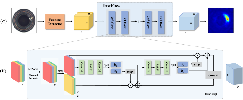
Figure 2: (a) the whole pipeline for unsupervised anomaly detection and localization in our method, which consists of a feature extractor and our FastFlow model. We can use an arbitrary network as the feature extractor such as CNN or vision transformer. FastFlow is alternatly stacked by the “$3\times 3$” and “$1\times 1$” flow. (b) one flow step for our FastFlow, the “Conv 2d” can be $3\times 3$ or $1\times 1$ convolution layer for $3\times 3$ or $1\times 1$ flow, respectively.

2.2 Feature extractors for Anomaly Detection

With the development of deep learning, recent unsupervised anomaly detection methods use deep neural networks as feature extractors, and produce more promising anomaly results. Most of them (Cohen and Hoshen 2020; Defard et al. 2020; Roth et al. 2021) use ResNet (He et al. 2016) to extract distinguish visual features. Some work has also begun to introduce ViT (Dosovitskiy et al. 2020) into unsupervised anomaly detection fields, such as VT-ADL (Mishra et al. 2021) uses vision transformer as backbone in a generated-based way. ViT has a global receptive field and can learn the relationship between global and local better. DeiT (Touvron et al. 2021a) and CaiT (Touvron et al. 2021b) are two typical models for ViT. DeiT introduces a teacher-student strategy specific to transformers, which makes image transformers learn more efficiently and got a new state-of-the-art performance. CaiT proposes a simple yet effective architecture designed in the spirit of encoder/decoder architecture and demonstrates that transformer models offer a competitive alternative to the best convolutional neural networks. In this paper, we use various networks belonging to CNN and ViT to prove the universality of our method.

2.3 Normalizing Flow

Normalizing Flows (NF) (Rezende and Mohamed 2015) are used to learn transformations between data distributions with special property that their transform process is bijective and the flow model can be used in both directions. Real-NVP (Dinh, Sohl-Dickstein, and Bengio 2016) and Glow (Kingma and Dhariwal 2018) are two typical methods for NF, in which both forward and reverse processes can be processed quickly. NF is generally used to generate data from variables sampled in a specific probability distribution, such as images or audios. Recently, some work (Rudolph, Wandt, and Rosenhahn 2021; Gudovskiy, Ishizaka, and Kozuka 2021) began to use it for unsupervised anomaly detection and localization. DifferNet (Rudolph, Wandt, and Rosenhahn 2021) achieved good image level anomaly detection performance by using NF to estimate the precise likelihood of test images. Unfortunately, this work failed to obtain the exact anomaly localization results since they flattened the outputs of feature extractor. CFLOW-AD (Gudovskiy, Ishizaka, and Kozuka 2021) proposes to use hard code position embedding to leverage the distribution learned by NF, which probably underperforms at more complicated datasets.

3 Methodology

In this section, we introduce the pipeline of our method and the architecture of the FastFlow, as shown in Figure 2. We first set up the problem definition of unsupervised anomaly detection, and introduce the basic methodology that uses a learnable probability density estimation model in the representation-based method. Then we describe the details of feature extractor and FastFlow models, respectively.

3.1 Problem Definition and Basic Methodology

Unsupervised anomaly detection is also denoted as one-class classification or out-of-distribution detection which requires the model to determines whether the test image is normal or abnormal. Anomaly localization requires a more fine-grained result that gives the anomalies label for each pixel. During the training stage, only normal images were observed, but the normal images and abnormal images simultaneously appear in inference. One of the mainstream methods is representation-based method which extracts discriminative feature vectors from normal images or normal image patches to construct the distribution and calculate anomaly score by the distance between the embedding of a test image and the distribution. The distribution is typically characterized by the center of an n-sphere for the normal image, the Gaussian distribution of normal images, or the normal embedding cluster stored in the memory bank obtained from KNN. After extract the features of the training dataset $D=\{x_{1},x_{2},\cdots,x_{N}\}$ where $x_{i},i=1,2,\cdots,N$ are samples from the distribution $p_{X}(x)$, a representation-based anomaly detection model $\mathcal{P}=\{P_{\theta}:\theta\in\Theta\}$ aims to learn the parameter $\theta$ in the parameter space $\Theta$ to map all $x_{i}$ from the raw distribution $p_{X}(x)$ into the same distribution $p_{Z}(z)$, with anomalous pixels or instances mapped out of the distribution. In our method, we follow this methodology and propose FastFlow $P_{\theta}$ to project the high-dimensional visual features of normal images extracted from typical backbone networks into the standard normal distribution.

3.2 Feature Extractor

In the whole pipeline of our method, we first extract the representative feature from the input image through ResNet or vision transformers. As mentioned in the Sec 1, one of significant challenges in the anomaly detection task is the global relation grasped to distinguish those abnormal regions from other local parts. Therefore, when using vision transformer (ViT) (Dosovitskiy et al. 2020) as the feature extractor, we only use the feature of one certain layer because ViT has stronger ability to capture the relationship between local patches and the global feature. For ResNet, we directly use the features of the last layer in the first three blocks, and put these features into three corresponding FastFlow model.

3.3 2D Flow Model

As shown in Figure 2, our 2D flow $f:X\rightarrow Z$ is used to project the image features $x\in p_{X}(x)$ into the hidden variable $z\in p_{Z}(z)$ with a bijective invertible mapping. For this bijection function, the change of the variable formula defines the model distribution on $X$ by:

$${p}_{X}(x)={p}_{Z}(z)\left|\mathbf{det}(\frac{\partial z}{\partial x})\right|$$ (1)

We can estimate the log likelihoods for image features from $p_{Z}(z)$ by:

$$\log{p}_{X}(x) =\log p_{Z}(z)+\log\left|\mathbf{det}(\frac{\partial z}{\partial x})\right|$$ (2)

$$=\log p_{Z}(f_{\theta}(x))+\log\left|\mathbf{det}(\frac{\partial f_{\theta}(x)}{\partial x})\right|,$$

where $z\sim\mathcal{N}(o,I)$ and the $\mathbf{\frac{\partial f_{\theta}(x)}{\partial x}}$ is the Jacobian of a bijective invertible flow model that $z=f_{\theta}(x)$ and $x=f^{-1}_{\theta}(z)$, $\theta$ is parameters of the 2D flow model. In inference, the features of anomalous images should be out of distribution and hence have lower likelihoods than normal images and the likelihood can be used as the anomaly score. Specifically, we sum the two-dimensional probabilities of each channel to get the final probability map and upsample it to the input image resolution using bilinear interpolation. In actual implementation, our flow model $f_{2d}$ is constructed by stacking multiple invertible transformations blocks $f_{i}$ in a sequence that:

$$X\xrightarrow{f_{1}}H_{1}\xrightarrow{f_{2}}H_{2}\xrightarrow{f_{3}}\cdots\xrightarrow{f_{K}}Z,$$

and

$$X\xleftarrow{f^{-1}_{1}}H_{1}\xleftarrow{f^{-1}_{2}}H_{2}\xleftarrow{f^{-1}_{3}}\cdots\xleftarrow{f^{-1}_{K}}Z,$$

where the 2D flow model is $f_{2d}=f_{1}\circ f_{2}\circ f_{3}\circ\cdots\circ f_{K}$ with $K$ transformation blocks. Each transformation block $f_{i}$ consists of multiple steps. Following (Dinh, Krueger, and Bengio 2014), we employ affine coupling layers in each block, and each step is formulated as follow:

$$y_{a},y_{b} =\text{split}(y)$$ (3)

$$y^{\prime}_{a} =y_{a}$$

$$y^{\prime}_{b} =s(y_{a})\odot y_{b}+b(y_{a})$$

$$y^{\prime} =\text{concat}(y^{\prime}_{a},y^{\prime}_{b}),$$

where $s(y_{a})$ and $b(y_{a})$ are outputs of two neural networks. The split($\cdot$) and concat($\cdot$) functions perform splitting and concatenation operations along the channel dimension. The two subnets s($\cdot$) and b($\cdot$) are usually implemented as fully connected networks in original normalizing flow model and need to flatten and squeeze the input visual features from 2D to 1D which destroy the spatial position relationship in the feature map. To convert the original normalizing flow to 2D manner, we adopt two-dimensional convolution layer in the default subnet to reserve spatial information in the flow model and adjust the loss function accordingly. In particular, we adopt a fully convolutional network in which 3$\times$3 convolution and 1$\times$1 convolution appear alternately, which reserves spatial information in the flow model.

Model	FPS	A.d. Time (ms)	A.d. Params (M)	Image-level AUC	Pixel-level AUC
CaiT-M48-distilled
+ Patch Core	2.39	107	0	97.9	96.5
+ CFlow	2.76	42	10.5	97.7	96.2
+ FastFlow	3.08	9	14.8	99.4	98.5
DeiT-base-distilled
+ Patch Core	15.45	39	0	96.5	97.9
+ CFlow	16.91	34	10.5	95.6	97.9
+ FastFlow	30.14	8	14.8	98.7	98.1
ResNet18
+ SPADE	3.92	250	0	-	-
+ CFlow	20.3	44	5.5	96.8	98.1
+ FastFlow	30.8	27	4.9	97.9	97.2
Wide-ResNet50-2
+ SPADE	0.67	1481	0	96.2	96.5
+ Patch Core	5.88	159	0	99.1	98.1
+ CFlow	14.9	56	81.6	98.3	98.6
+ FastFlow	21.8	34	41.3	99.3	98.1

Table 1: Complexity comparison in terms of inference speed (FPS), additional inference time (millisecond) and number of additional parameters (M) for various backbones. A.d. Time means the additional inference time and A.d. Parmas is the number of additional parameters compared with backbone network.

4 Experiments

4.1 Datasets and Metrics

We evaluate the proposed method on three datasets: MVTec AD (Bergmann et al. 2019), BTAD (Mishra et al. 2021) and CIFAR-10 (Krizhevsky, Hinton et al. 2009). MVTec AD and BTAD are both industrial anomaly detection datasets with pixel-level annotations, which are used for anomaly detection and localization. CIFAR-10 is built for image classification and we use it to do anomaly detection. Following the previous works, we choose one of the categories as normal, and the rest as abnormal. The anomalies in these industrial datasets are finer than those in CIFAR-10, and the anomalies in CIFAR-10 are more related to the semantic high-level information. For example, the anomalies in MVTec AD are defined as small areas, while the anomalies in CIFAR-10 dataset are defined as different object categories. Under the unsupervised setting, we train our model for each category with its respective normal images and evaluate it in test images that contain both normal and abnormal images.

The performance of the proposed method and all comparable methods is measured by the area under the receiver operating characteristic curve (AUROC) at image or pixel level. For the detection task, evaluated models are required to output single score (anomaly score) for each input test image. In the localization task, methods need to output anomaly scores for every pixel.

4.2 Complexity Analysis

We make a complexity analysis of FastFlow and other methods from aspects of inference speed, additional inference time and additional model parameters, “additional” refers to not considering the backbone itself. The hardware configuration of the machine used for testing is Intel(R) Xeon(R) CPU E5-2680 V4@2.4GHZ and NVIDIA GeForce GTX 1080Ti. SPADE and Patch Core perform KNN clustering between each test feature of each image patch and the gallery features of normal image patches, and they do not need to introduce parameters other than backbone. CFlow avoids the time-consuming k-nearest-neighbor-search process, but it still needs to perform testing phase in the form of a slice window. Our FastFlow adopts an end-to-end inference phase which has high efficiency of inference. The analysis results are shown in Table 1, we can observe that our method is up to $10\times$ faster than other methods. Compared with CFlow which also uses flow model, our method achieves $1.5\times$ speedup and $2\times$ parameter reduction. When using vision transformers (deit and cait) as the feature extractor, our FastFlow can achieve 99.4 image-level AUC for anomaly detection which is superior to CFlow and Patch Core. From the perspective of additional inference time, our method achieves up to $4\times$ reduction compared to Cflow and $10\times$ reduction compared to Patch Core. Our FastFlow can still have a competitive performance when using ResNet model as feature extractor.

Method	PatchSVDD	SPADE*	DifferNet	PaDiM	Cut Paste	PatchCore	CFlow	FastFlow
carpet	(92.9,92.6)	(98.6,97.5)	(84.0,-)	(-,99.1)	(100.0,98.3)	(98.7,98.9)	(100.0,99.3)	(100.0,99.4)
grid	(94.6,96.2)	(99.0,93.7)	(97.1,-)	(-,97.3)	(96.2,97.5)	(98.2,98.7)	(97.6,99.0)	(99.7,98.3)
leather	(90.9,97.4)	(99.5,97.6)	(99.4,-)	(-,99.2)	(95.4,99.5)	(100.0,99.3)	(97.7,99.7)	(100.0,99.5)
tile	(97.8,91.4)	(89.8,87.4)	(92.9,-)	(-,94.1)	(100.0,90.5)	(98.7,95.6)	(98.7,98.0)	(100.0,96.3)
wood	(96.5,90.8)	(95.8,88.5)	(99.8,-)	(-,94.9)	(99.1,95.5)	(99.2,95.0)	(99.6,96.7)	(100.0,97.0)
bottle	(98.6,98.1)	(98.1,98.4)	(99.0,-)	(-,98.3)	(99.9,97.6)	(100.0,98.6)	(100.0,99.0)	(100.0,97.7)
cable	(90.3,96.8)	(93.2,97.2)	(86.9,-)	(-,96.7)	(100.0,90.0)	(99.5,98.4)	(100.0,97.6)	(100.0,98.4)
capsule	(76.7 ,95.8)	(98.6,99.0)	(88.8,-)	(- ,98.5)	(98.6 ,97.4)	(98.1,98.8)	(99.3 ,99.0)	(100.0,99.1)
hazelnut	(92.0 ,97.5)	(98.9,99.1)	(99.1,-)	(- ,98.2)	(93.3 ,97.3)	(100.0,98.7)	(96.8 ,98.9)	(100.0,99.1)
meta nut	(94.0,98.0)	(96.9,98.1)	(95.1,-)	(-,97.2)	(86.6,93.1)	(100.0,98.4)	(91.9,98.6)	(100.0,98.5)
pill	(86.1,95.1)	(96.5,96.5)	(95.9,-)	(-,95.7)	(99.8,95.7)	(96.6,97.1)	(99.9,99.0)	(99.4,99.2)
screw	(81.3,95.7)	(99.5,98.9)	(99.3,-)	(-,98.5)	(90.7,96.7)	(98.1,99.4)	(99.7,98.9)	(97.8,99.4)
toothbrush	(100.0,98.1)	(98.9,97.9)	(96.1,-)	(-,98.8)	(97.5 ,98.1)	(100.0,98.7)	(95.2,99.0)	(94.4 ,98.9)
transistor	(91.5,97.0)	(81.0,94.1)	(96.3,-)	(-,97.5)	(99.8,93.0)	(100.0,96.3)	(99.1 ,98.0)	(99.8,97.3)
zipper	(97.9,95.1)	(98.8,96.5)	(98.6,-)	(-,98.5)	(99.9,99.3)	(98.8,98.8)	(98.5 ,99.1)	(99.5,98.7)
AUCROC	(92.1,95.7)	(96.2,96.5)	(94.9,-)	(97.9,97.5)	(97.1,96.0)	(99.1,98.1)	(98.3,98.6)	(99.4,98.5)

Table 2: Anomaly detection and localization performance on MVTec AD dataset with the format (image-level AUC, pixel-level AUC). We report the detailed results for all categories.

4.3 Quantitative Results

MVTec AD

There are 15 industrial products in MVTec AD dataset (Bergmann et al. 2019), with a total of 5,354 images, among which 10 are objects and the remaining 5 are textures. The training set is only composed of normal images, while the test set is a mixture of normal images and abnormal images. We compare our proposed method with the state-of-the-art anomaly detection works, including SPADE* (Reiss et al. 2021), PatchSVDD (Yi and Yoon 2020), DifferNet (Rudolph, Wandt, and Rosenhahn 2021), Mah.AD (Rippel, Mertens, and Merhof 2021), PaDiM (Defard et al. 2020), Cut Paste (Li et al. 2021), Patch Core (Roth et al. 2021), CFlow (Gudovskiy, Ishizaka, and Kozuka 2021) under the metrics of image-level AUC and pixel-level AUC. The detailed comparison results of all categories are shown in Table 2. We can observe that FastFlow achieves 99.4 AUC on image-level and 98.5 AUC on pixel-level, suppresses all other methods in anomaly detection task.

Categories	AE MSE	AE MSE+SSIM	VT-ADL	FastFlow
0	0.49	0.53	0.99	0.95
1	0.92	0.96	0.94	0.96
2	0.95	0.89	0.77	0.99
Mean	0.78	0.79	0.90	0.97

Table 3: Anomaly localization results on BTAD datasts. We compare our method with convolutional auto encoders trained with MSE-loss and MSE+SSIM loss, and VT-ADL.

BTAD

BeanTech Anomaly Detection dataset (Mishra et al. 2021) has 3 categories industrial products with 2540 images. The training set consists only of normal images, while the test set is a mixture of normal images and abnormal images. Under the measure of pixel-level AUC, we compare the results of our FastFlow with the results of three methods reported in VT-ADL (Mishra et al. 2021): auto encoder with mean square error, automatic encoder with SSIM loss and VT-ADL. The comparison results are shown in Table 3. We can observe that our FastFlow achieves 97.0 pixel-wise AUC and suppresses other methods as high as 7% AUC.

Method	OC-SVM	KDE	$\textit{l}_{2}$-AE	VAE	Pixel CNN
AUC	58.6	61.0	53.6	58.3	55.1
Method	LSA	AnoGAN	DSVDD	OCGAN	FastFlow
AUC	64.1	61.8	64.8	65.6	66.7

Table 4: Anomaly detection results on CIFAR-10 datast.

CIFAR-10 dataset

CIFAR-10 has 10 categories with 60000 natural images. Under the setting of anomaly detection, one category is regarded as anomaly and other categories are used as normal data. And we need to train the corresponding model for each class respectively. The AUC scores of our method and other methods are reported in Table 4. Methods for comparison includes OC-SVM (Schölkopf et al. 1999), KDE (Bishop 2006), $\textit{l}_{2}$-AE (Hadsell, Chopra, and LeCun 2006), VAE (An and Cho 2015), Pixel CNN (Oord et al. 2016), LSA (Abati et al. 2019), AnoGAN (Schlegl et al. 2017), DSVDD (Ruff et al. 2018) and OCGAN (Perera, Nallapati, and Xiang 2019). Our method outperforms these comparison methods. The results in three different datasets show that our method can adapt to different anomaly detection settings.

4.4 Ablation Study

To investigate the effectiveness of the proposed FastFlow structure, we design ablation experiments about the convolution kernel selection in subnet. We compare alternately using $3\times 3$ and $1\times 1$ convolution kernel and only using $3\times 3$ kernel under the AUC and inference speed for the subnet with various backbone networks. The results are shown in Table 5. For the backbone network with large model capacities such as CaiT and Wide-ResNet50-2, alternate using $3\times 3$ and $1\times 1$ convolution layer can obtain higher performance while reducing the amount of parameters. For the backbone network with small model capacities such as DeiT and ResNet18, only using $3\times 3$ convolution layer has higher performance. To achieve the balance of accuracy and inference speed, we use alternate convolution kernels of $3\times 3$, $1\times 1$ with DeiT, CaiT and Wide-ResNet50-2, and only use $3\times 3$ convolution layer with ResNet18.

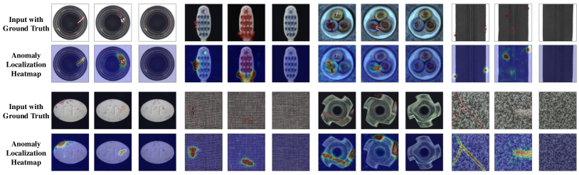
Figure 3: Anomaly localization results of MVTec AD datasets. From top to bottom, input images with ground-truth localization area labeled in red and anomaly localization heatmaps.

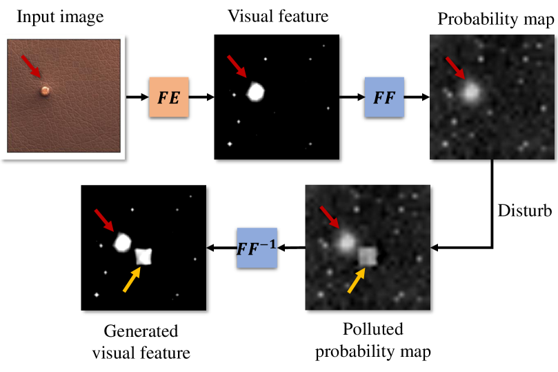
Figure 4: The bidirectional invertible process for FastFlow. “FE” is the feature extractor, “FF” is our FastFlow model, “$\text{FF}^{-1}$” is the reverse for FastFlow. The red and yellow arrows point to the original anomaly and the new anomaly introduced after the noise disturbance respectively.

4.5 Feature Visualization and Generation.

Our FastFlow model is a bidirectional invertible probability distribution transformer. In the forward process, it takes the feature map from the backbone network as input and transforms its original distribution into a standard normal distribution in two-dimensional space. In the reverse process, the inverse of FastFlow can generate the visual feature from a specific probability sampling variable. To better understand this ability in view of our FastFlow, we visualize the forward (from visual features to probability map) and reverse (from probability map to visual features) processes. As shown in Figure 4, we extract the features of an input image belonging to the leather class and the abnormal area is indicated by the red arrow. We forward it through the FastFlow model to obtain the probability map. Our FastFlow successfully transformed the original distribution into the standard normal distribution. Then, we add noise interference to a certain spatial area which is indicated by the yellow arrow in this probability map, and generate a leather feature tensor from the pollution probability map by using the inverse Fastflow model. In which we visualized the feature map of one channel in this feature tensor, and we can observe that new anomaly appeared in the corresponding pollution position.

Method	A.d. Params (M)	Image-level AUC	Pixel-level AUC
DeiT
3-1	14.8	98.7	98.1
3-3	26.6	98.7	98.3
CaiT
3-1	14.8	99.4	98.5
3-3	26.6	98.9	98.5
ResNet18
3-1	2.7	97.3	96.8
3-3	4.9	97.9	97.2
Wide-ResNet50-2
3-1	41.3	99.3	98.1
3-3	74.4	98.2	97.6

Table 5: Results of ablation experiments with various backbone networks. 3-1 means alternately using $3\times 3$ and $1\times 1$ convolution layers and 3-3 is only using $3\times 3$ convolution layer in the subnet for FastFlow. A.d. Params is the number of additional model parameters compared with backbone network.

4.6 Qualitative Results

We visualize some results of anomaly detection and localization in Figure 3 with the MVTec AD dataset. The top row shows test images with ground truth masks with and without anomalies, and the anomaly localization score heatmap is shown in the bottom row. There are both normal and abnormal images and our FastFlow gives accurate anomaly localization results.

Backbone	Input Size	Block Index	Feature Size
CaiT-M48-distilled	448	40	28
DeiT-base-distilled	384	7	24
Res18	256	[1,2,3]	[64, 32, 16]
WR50	256	[1,2,3]	[64, 32, 16]

Table 6: We use four different feature extractors in all experiments. The input picture size and feature size are set according to the backbone network and the block index indicates the block from which the feature is obtained..

4.7 Implementation Details

We provide the details of the structure of feature extractor, the selection of feature layer and the size of input image in Table 6. For vision transformer, our method only uses feature maps of a specific layer, and does not need to design complicated multi-scale features manually. For ResNet18 and Wide-ResNet50-2, we directly use the features of the last layer in the first three blocks, put these features into the 2D flow model to obtain their respective anomaly detection and localization results, and finally take the average value as the final result. All these backbone are initialized with the ImageNet pre-trained weights and their parameters are frozen in the following training process. For FastFlow, we use 20-step flows in CaiT and DeiT and 8-step flows for ResNet18 and Wide-ResNet50-2. We train our model using Adam optimizer with the learning rate of 1e-3 and weight decay of 1e-5. We use a 500 epoch training schedule, and the batch size is 32.

5 Conclusion

In this paper, we propose a novel approach named FastFlow for unsupervised anomaly detection and localization. Our key observation is that anomaly detection and localization requires comprehensive consideration of global and local information with a learnable distribution modeling method, and efficient inference process, which are ignored in the existing approaches. To this end, we present a 2D flow model denoted as FastFlow which has a lightweight structure and is used to project the feature distribution of normal images to the standard normal distribution in training, and use the probabilities as the anomaly score in testing. FastFlow can be used in typical feature extraction networks such as ResNet and ViT in the form of plug-ins. Extensive experimental results on MVTec AD dataset show FastFlow superiority over the state-of-the art methods in terms of accuracy and reasoning efficiency.

Supplementary Material for
FastFlow: Unsupervised Anomaly Detection and Localization via 2D Normalizing Flows

6 More Ablation Studies

6.1 Channels of Hidden Layers in Flow Model

In the original flow model which has been used in DifferNet (Rudolph, Wandt, and Rosenhahn 2021) and CFLOW (Gudovskiy, Ishizaka, and Kozuka 2021), the number of channels of hidden layers in all subnet is set to $2\times$ as much the input and output layer’s channel. This kind of design improves the results by increasing the complexity of the model, but it reduces the efficiency of inference. In our FastFlow, we found that using $0.16\times$ number of channels in CaiT and $1\times$ number of channels in Wide-ResNet50-2 can achieve a balance between performance and model parameters. In addition, when we use $0.25\times$ number of channels of Wide-ResNet50-2, we can further reduce the model parameters while still maintaining high accuracy. The results are shown in Table 7.

Channel Ratio	Parameters (M)	Image-level AUC	Pixel-level AUC
CaiT
$0.16\times$	14.8	99.4	98.5
$0.33\times$	29.6	98.9	98.4
Wide-ResNet50-2
$0.25\times$	10.9	98.9	98.0
$0.5\times$	20.7	99.1	98.1
$1.0\times$	41.3	99.3	98.1
$2.0\times$	82.6	99.4	98.1

Table 7: Ablation study results about the hidden layer channels for CNN and vision transformer in MVTec AD dataset. Channel Ratio means the ratio of the number of channels in the hidden layer to the number of channels in the input and output layers for subnet in our FastFlow.

6.2 Training Data Augmentation

In order to learn a more robust FastFlow model, we apply various data augmentation methods to the MVTec AD dataset during the training phase. We use random horizontal flip, vertical flip and rotation, with probabilities of 0.5, 0.3 and 0.7, respectively. It should be noted that some categories are not suitable for violent data augmentation. For example, the transistor can not be flipped upside down and rotated. The results are shown in Table 8.

Data Augmentation	Image-level AUC	Pixel-level AUC
CaiT
w/o	99.3	98.4
w	99.4	98.5
Wide-ResNet50-2
w/o	98.9	98.2
w	99.3	98.1

Table 8: The effect of data augmentation on the anomaly detection and localization performance.

7 Bad Cases and Ambiguity Label

We visualize bad cases for our method on MVTec AD dataset in Figure 5 to Figure 7 which are summarized into three categories. We show the missing detection cases in Figure 5, false detection cases in Figure 6 and label ambiguity cases in Figure 7. In Figure 5, our method missed a few small and unobvious anomalies. In Figure 6, our method had false detection results in some background areas, such as areas with hair and dirt in the background. In Figure 7, our method found some areas belong to abnormal but not be labeled, such as the “scratch neck” for screw and the “fabric interior” for zipper.

8 Non-aligned Disturbed MVTec AD Dataset

Considering that the MVTec AD dataset has the characteristic of sample alignment which is infrequent in practical application, we perform a series of spatial perturbations on the test data to obtain an unaligned MVTec AD dataset. In detail, we apply random zoom in/out with 0.85 ratio, random rotation with $\pm 15$ angle, random translation with 0.15 ratio to expand the original test dataset by $4\times$ to the new test dataset. We evaluate our FastFlow (with CaiT) in this new test dataset and we obtain 99.2 image-level AUC and 98.1 pixle-level AUC. There is almost no performance loss compared with the results in original aligned MVTec AD test dataset, which proves the robustness of our method. We also give some visualization results in Figure 8. We can observe that FastFlow can still have high performance on anomaly detection and location result in this non-aligned disturbed MVTec AD dataset.

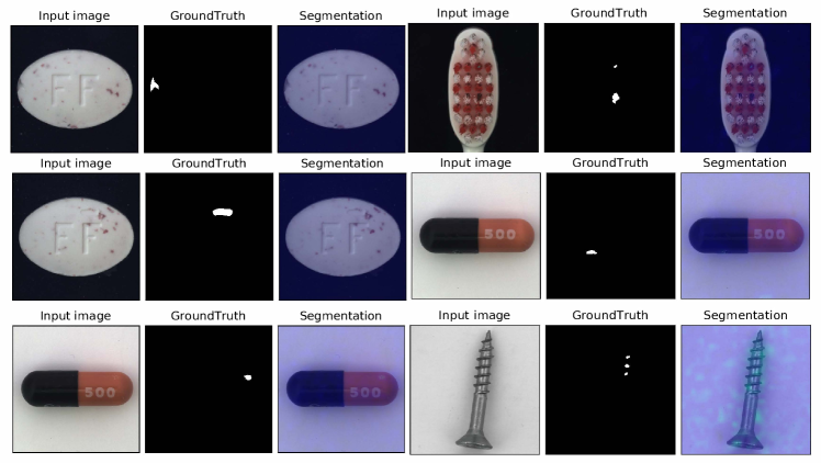
Figure 5: Bad cases of the missing detection type. All missed detection results of our method in shown in this figure.

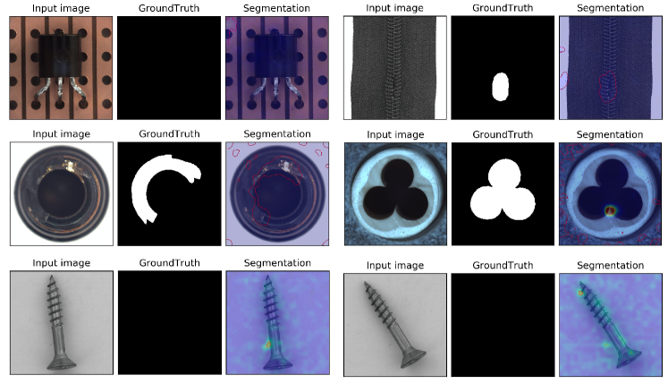
Figure 6: Bad cases of false detection type. We give the typical results of our method in this figure.

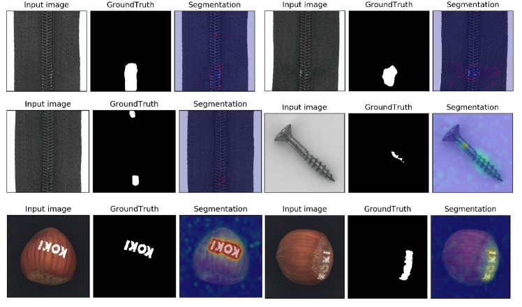
Figure 7: Bad cases caused by label ambiguity. In the first two rows, there are abnormal areas localized by our method while not labeled. In the last row of hazelnut, we show the label ambiguity of the “print” subclass, in which one hazelnut print is labeled finely, while the other is labeled with a rough area.

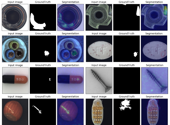
Figure 8: Anomaly localization results of the non-aligned disturbed MVTec AD datasets.

References

- Abati et al. (2019) Abati, D.; Porrello, A.; Calderara, S.; and Cucchiara, R. 2019. Latent space autoregression for novelty detection. In Proceedings of the IEEE/CVF Conference on Computer Vision and Pattern Recognition, 481–490.
- An and Cho (2015) An, J.; and Cho, S. 2015. Variational autoencoder based anomaly detection using reconstruction probability. Special Lecture on IE, 2(1): 1–18.
- Bergman and Hoshen (2020) Bergman, L.; and Hoshen, Y. 2020. Classification-based anomaly detection for general data. International Conference on Learning Representations (ICLR).
- Bergmann et al. (2019) Bergmann, P.; Fauser, M.; Sattlegger, D.; and Steger, C. 2019. MVTec AD – A Comprehensive Real-World Dataset for Unsupervised Anomaly Detection. In Proceedings of the IEEE/CVF Conference on Computer Vision and Pattern Recognition, 9592–9600.
- Bishop (2006) Bishop, C. M. 2006. Pattern recognition. Machine learning, 128(9).
- Cohen and Hoshen (2020) Cohen, N.; and Hoshen, Y. 2020. Sub-image anomaly detection with deep pyramid correspondences. arXiv preprint arXiv:2005.02357.
- Defard et al. (2020) Defard, T.; Setkov, A.; Loesch, A.; and Audigier, R. 2020. PaDiM: a Patch Distribution Modeling Framework for Anomaly Detection and Localization. arXiv preprint arXiv:2011.08785.
- Dinh, Krueger, and Bengio (2014) Dinh, L.; Krueger, D.; and Bengio, Y. 2014. Nice: Non-linear independent components estimation. arXiv preprint arXiv:1410.8516.
- Dinh, Sohl-Dickstein, and Bengio (2016) Dinh, L.; Sohl-Dickstein, J.; and Bengio, S. 2016. Density estimation using real nvp. arXiv preprint arXiv:1605.08803.
- Dosovitskiy et al. (2020) Dosovitskiy, A.; Beyer, L.; Kolesnikov, A.; Weissenborn, D.; Zhai, X.; Unterthiner, T.; Dehghani, M.; Minderer, M.; Heigold, G.; Gelly, S.; et al. 2020. An image is worth 16x16 words: Transformers for image recognition at scale. arXiv preprint arXiv:2010.11929.
- Gong et al. (2019) Gong, D.; Liu, L.; Le, V.; Saha, B.; Mansour, M. R.; Venkatesh, S.; and Hengel, A. v. d. 2019. Memorizing normality to detect anomaly: Memory-augmented deep autoencoder for unsupervised anomaly detection. In Proceedings of the IEEE/CVF International Conference on Computer Vision, 1705–1714.
- Gudovskiy, Ishizaka, and Kozuka (2021) Gudovskiy, D.; Ishizaka, S.; and Kozuka, K. 2021. CFLOW-AD: Real-Time Unsupervised Anomaly Detection with Localization via Conditional Normalizing Flows. arXiv preprint arXiv:2107.12571.
- Hadsell, Chopra, and LeCun (2006) Hadsell, R.; Chopra, S.; and LeCun, Y. 2006. Dimensionality reduction by learning an invariant mapping. In 2006 IEEE Computer Society Conference on Computer Vision and Pattern Recognition (CVPR’06), volume 2, 1735–1742. IEEE.
- He et al. (2016) He, K.; Zhang, X.; Ren, S.; and Sun, J. 2016. Deep residual learning for image recognition. In Proceedings of the IEEE conference on computer vision and pattern recognition, 770–778.
- Kingma and Dhariwal (2018) Kingma, D. P.; and Dhariwal, P. 2018. Glow: Generative flow with invertible 1x1 convolutions. arXiv preprint arXiv:1807.03039.
- Krizhevsky, Hinton et al. (2009) Krizhevsky, A.; Hinton, G.; et al. 2009. Learning multiple layers of features from tiny images.
- Li et al. (2021) Li, C.-L.; Sohn, K.; Yoon, J.; and Pfister, T. 2021. CutPaste: Self-Supervised Learning for Anomaly Detection and Localization. arXiv preprint arXiv:2104.04015.
- Mishra et al. (2021) Mishra, P.; Verk, R.; Fornasier, D.; Piciarelli, C.; and Foresti, G. L. 2021. VT-ADL: A Vision Transformer Network for Image Anomaly Detection and Localization. arXiv preprint arXiv:2104.10036.
- Oord et al. (2016) Oord, A. v. d.; Kalchbrenner, N.; Vinyals, O.; Espeholt, L.; Graves, A.; and Kavukcuoglu, K. 2016. Conditional image generation with pixelcnn decoders. arXiv preprint arXiv:1606.05328.
- Perera, Nallapati, and Xiang (2019) Perera, P.; Nallapati, R.; and Xiang, B. 2019. Ocgan: One-class novelty detection using gans with constrained latent representations. In Proceedings of the IEEE/CVF Conference on Computer Vision and Pattern Recognition, 2898–2906.
- Reiss et al. (2021) Reiss, T.; Cohen, N.; Bergman, L.; and Hoshen, Y. 2021. PANDA: Adapting Pretrained Features for Anomaly Detection and Segmentation. In Proceedings of the IEEE/CVF Conference on Computer Vision and Pattern Recognition, 2806–2814.
- Rezende and Mohamed (2015) Rezende, D.; and Mohamed, S. 2015. Variational inference with normalizing flows. In International conference on machine learning, 1530–1538. PMLR.
- Rippel, Mertens, and Merhof (2021) Rippel, O.; Mertens, P.; and Merhof, D. 2021. Modeling the distribution of normal data in pre-trained deep features for anomaly detection. In 2020 25th International Conference on Pattern Recognition (ICPR), 6726–6733. IEEE.
- Roth et al. (2021) Roth, K.; Pemula, L.; Zepeda, J.; Schölkopf, B.; Brox, T.; and Gehler, P. 2021. Towards Total Recall in Industrial Anomaly Detection. arXiv preprint arXiv:2106.08265.
- Rudolph, Wandt, and Rosenhahn (2021) Rudolph, M.; Wandt, B.; and Rosenhahn, B. 2021. Same same but differnet: Semi-supervised defect detection with normalizing flows. In Proceedings of the IEEE/CVF Winter Conference on Applications of Computer Vision, 1907–1916.
- Ruff et al. (2018) Ruff, L.; Vandermeulen, R.; Goernitz, N.; Deecke, L.; Siddiqui, S. A.; Binder, A.; Müller, E.; and Kloft, M. 2018. Deep one-class classification. In International conference on machine learning, 4393–4402. PMLR.
- Schlegl et al. (2017) Schlegl, T.; Seeböck, P.; Waldstein, S. M.; Schmidt-Erfurth, U.; and Langs, G. 2017. Unsupervised anomaly detection with generative adversarial networks to guide marker discovery. In International conference on information processing in medical imaging, 146–157. Springer.
- Schölkopf et al. (1999) Schölkopf, B.; Williamson, R. C.; Smola, A. J.; Shawe-Taylor, J.; Platt, J. C.; et al. 1999. Support vector method for novelty detection. In NIPS, volume 12, 582–588. Citeseer.
- Touvron et al. (2021a) Touvron, H.; Cord, M.; Douze, M.; Massa, F.; Sablayrolles, A.; and Jégou, H. 2021a. Training data-efficient image transformers & distillation through attention. In International Conference on Machine Learning, 10347–10357. PMLR.
- Touvron et al. (2021b) Touvron, H.; Cord, M.; Sablayrolles, A.; Synnaeve, G.; and Jégou, H. 2021b. Going deeper with image transformers. arXiv preprint arXiv:2103.17239.
- Wang et al. (2021) Wang, S.; Wu, L.; Cui, L.; and Shen, Y. 2021. Glancing at the Patch: Anomaly Localization With Global and Local Feature Comparison. In Proceedings of the IEEE/CVF Conference on Computer Vision and Pattern Recognition, 254–263.
- Yan et al. (2021) Yan, X.; Zhang, H.; Xu, X.; Hu, X.; and Heng, P.-A. 2021. Learning Semantic Context from Normal Samples for Unsupervised Anomaly Detection. In Proceedings of the AAAI Conference on Artificial Intelligence, volume 35, 3110–3118.
- Yi and Yoon (2020) Yi, J.; and Yoon, S. 2020. Patch SVDD: Patch-level SVDD for Anomaly Detection and Segmentation. In Proceedings of the Asian Conference on Computer Vision.