Joint FCLT for Sample Quantile and Measures of Dispersion for Functionals of Mixing Processes

?abstractname?

In this paper, we establish a joint (bivariate) functional central limit theorem of the sample quantile and the $r$-th absolute centred sample moment for functionals of mixing processes. More precisely, we consider $L_{2}$-near epoch dependent processes that are functionals of either $\phi$-mixing or absolutely regular processes. The general results we obtain can be used for two classes of popular and important processes in applications: The class of augmented GARCH($p$,$q$) processes with independent and identically distributed innovations (including many GARCH variations used in practice) and the class of ARMA($p$,$q$) processes with mixing innovations (including, e.g., ARMA-GARCH processes). For selected examples, we provide exact conditions on the moments and parameters of the process for the joint asymptotics to hold.

2010 AMS classification: 60F05; 60F17; 60G10; 62H10; 62H20
JEL classification: C13; C14; C30
Keywords: asymptotic distribution; Bahadur representation; functional central limit theorem; near epoch dependence; mixing; (augmented) GARCH; ARMA; dependence; (sample) quantile; measure of dispersion; (sample) mean absolute deviation; (sample) variance

1 Introduction and framework

The focus of this paper is on the asymptotic theory of sample estimators of standard statistical quantities as rank, location and dispersion measures, for a very large class of widely used stationary processes. Such a theory is often needed for related statistical inference. The literature for sample quantiles has considerably developed (closely related to empirical processes) from the iid setting toward dependent random variables. In view of applications, it is also important to consider jointly the estimators of such standard statistical quantities. Fields of applications include dynamic systems (networks), (financial) econometrics, reliability, risk theory and management, quantitative finance, etc. For instance, dispersion measures, as e.g. the 2nd centred moment (named volatility in financial fields), are essential in economics for studying market fluctuations. This is why they are often introduced, via conditioning or jointly, in the econometric analysis of macroeconomic and financial data, to take into account the market state. Investigations on the relation between volatility estimators (a measure of dispersion) and Value-at-Risk (a quantile estimator) for time-series models are common in this field; see e.g. [14],[27],  [38], [66, 67].

In the literature, the asymptotic behavior of each quantity has been investigated on its own, under some dependence structures. Limit theorems for sample quantiles have been proposed, inter alia, in the case of m-dependent or $\phi$-mixing processes ([53], [54]), infinite-variance or non-linear processes ([30], [63]), and functionals of mixing processes ([61]). They are generally based on the use of the Bahadur representation developed in [4] for independent and identically distributed (iid) random variables (and refined by Kiefer in a sequence of papers), then extended (generally via coupling techniques) to linear and nonlinear processes, with various types of dependence (see e.g. [63, 64] and references therein).

For dispersion measures, there exist results for the mean absolute deviation (MAD) when considering strongly mixing processes ([52]), while the asymptotics of the sample variance can be found for various settings as examples in standard textbooks, see e.g. [1], [15], [58]. When considering more generally the autocovariance function of such estimators, we can mention, exemplarily, results for linear, bilinear or non-linear processes with regularly varying noise ([18], [19]), and for long-memory time series (e.g. [35] - and for a more complete overview [39] and references therein).

In this paper, we establish the joint asymptotics of the sample quantile and the $r$-th absolute centred sample moment for functionals of strictly stationary processes $(Z_{n})_{n\in\mathbb{Z}}$, namely

$$X_{n}=f(Z_{n+k},k\in\mathbb{Z}),\quad\text{with $f$ measurable,}$$

assuming $(Z_{n})$ $\phi$-mixing or absolutely regular, respectively, and $(X_{n})$ near-epoch dependent. We briefly recall these dependence notions further below. Our limit theorem extends existing results on joint asymptotics in the case of an identically and independently distributed (iid) sample (see [14]). In particular, we establish an asymptotic representation for the $r$-th absolute centred sample moment for stationary, ergodic, short-memory processes under minimal conditions (extending the results in [52] and [14]). Furthermore, our general results include two important popular classes of linear and nonlinear processes: The class of augmented GARCH($p$,$q$) processes with iid innovations and ARMA($p$,$q$) processes with mixing innovations. The former, introduced by Duan in [23], contains many well-known GARCH processes as special cases, of standard use, e.g. in quantitative finance and financial econometrics. Previous works on univariate CLTs and stationarity conditions for this class of GARCH processes are, among others, [3],[5],[34] and [40]. The class of ARMA processes includes the classical ARMA models with iid or white noise innovations (see e.g. [15], [12] for classical references on the topic), but also with mixing inovations. The earliest explicitly mentioned examples of ARMA processes with mixing innovations date back, to our knowledge, to [59], [60] considering ARMA models with ARCH errors. More widespreadly used in applications is the ARMA-GARCH model, which can be seen as an extension of the GARCH models to also have dynamics in the mean and not only in the variance process. First contributions on such types of processes can be found in [43], [44], [46]; more recent examples of applications are, e.g. [32, 55, 56]. Analogously to the class of augmented GARCH processes, there exist results in the literature on FCLTs for ARMA processes with mixing innovations (or even larger classes of linear processes), as e.g. [17], [50].

Classical and broad notions for (asymptotically vanishing) dependence of a process are known under the name of mixing (see [13] for an overview). Let us recall some notions of weak dependence related to the mixing coefficients. Let $(Y_{n})_{n\in\mathbb{Z}}$ be a random process and denote the corresponding $\sigma$-algebra as $\mathcal{F}_{Y,s,t}=\sigma(Y_{u};s\leq u\leq t)$.

Definition 1 (Mixing coefficients).

For any integer $n\geq 1$, let

$$\alpha(n) :=\sup_{j\in\mathbb{Z}}\;\sup_{C\in\mathcal{F}_{Y,-\infty,j},D\in\mathcal{F}_{Y,j+n,\infty}}\lvert P(C\cap D)-P(C)P(D)\rvert,$$

$$\beta(n) :=\sup_{j\in\mathbb{Z}}\;\operatorname{\mathbb{E}}[\sup_{C\in\mathcal{F}_{Y,j+n,\infty}}\lvert P(C|\mathcal{F}_{Y,-\infty,j})-P(C)\rvert],$$

$$\phi(n) :=\sup_{j\in\mathbb{Z}}\;\sup_{C\in\mathcal{F}_{Y,-\infty,j}:P(C)>0,D\in\mathcal{F}_{Y,j+n,\infty}}\lvert P(D|C)-P(D)\rvert.$$

The process $(Y_{n})_{n\in\mathbb{Z}}$ is called strongly mixing if $\displaystyle\alpha(n)\underset{n\to\infty}{\rightarrow}0$, $\displaystyle\beta$-mixing or absolutely regular if $\beta(n)\underset{n\to\infty}{\rightarrow}0$, and $\phi$-mixing if $\phi(n)\underset{n\to\infty}{\rightarrow}0$.

Note that, for a stationary time series, we can omit the $\displaystyle\sup_{j\in\mathbb{Z}}$ in the definition of the mixing notions and simply set, w.l.o.g. , $j=0$. Also, $\phi$-mixing implies $\beta$-mixing that implies $\alpha$-mixing, but the converse does not hold in general.

A drawback of mixing is that, in general, a functional that depends on an infinite number of lags of a mixing process will not be mixing itself. This gave rise to the introduction of the notion of $L_{p}$-near-epoch dependence ($L_{p}$-NED) (that goes back to [37] in the case of $p=2$ for an underlying $\phi$-mixing process, even if not named NED there). It imposes additional structure on functionals of mixing processes enabling statistical inference for this larger class of processes. Alternatively, $L_{p}$-NED is also called $p$-approximation functional; see [9], [61].

Definition 2 ($L_{p}$-NED, [2]).

For $p>0$, a stationary process $(X_{n})_{n\in\mathbb{Z}}$ is called $L_{p}$-NED on a process $\left(Z_{n}\right)_{n\in\mathbb{Z}}$ if, for $k\geq 0$,

$$\|X_{0}-\operatorname{\mathbb{E}}[X_{0}|\mathcal{F}_{Z,-k,+k}]\|_{p}\leq\nu(k),$$

for non-negative constants $\nu(k)$ such that $\nu(k)\rightarrow 0$ as $k\rightarrow\infty$.

Note that, in the econometrics literature, a specific terminology is used for the rate of $\nu(k)$: If $\nu(k)=O(k^{-\tau-\epsilon})$ for some $\epsilon>0$, one calls the process $L_{p}$-NED of size $\left(-\tau\right)$ and, if $\nu(k)=O(e^{-\delta k})$ for some $\delta>0$, geometrically $L_{p}$-NED.

Finally, let us present some technical conditions on the marginal distribution function $F_{X}$ of the stationary process $(X_{n})_{n\in\mathbb{Z}}$ under study, and give the notation of the sample estimators for the two quantities of interest. We denote, whenever they exist, the probability density function (pdf) of $F_{X}$ by $f_{X}$, with mean $\mu$, variance $\sigma^{2}$, as well as, for any integer $r\geq 1$, the $r$-th absolute centred moment, $\mu(X,r):=\operatorname{\mathbb{E}}[\lvert X_{0}-\mu\rvert^{r}]$. The quantile of order $p$ of $F_{X}$ is defined as $q_{X}(p):=\inf\{x\in\mathbb{R}:F_{X}(x)\geq p\}$.

We impose four different types of conditions on the marginal distribution $F_{X}$, as in the iid case (see [14]). First, we assume the existence of its finite $2k$-th moment for any integer $k>0$. Then, the continuity or $l$-fold differentiability of $F_{X}$ (at a given point or neighbourhood) for any integer $l>0$, and the positivity of $f_{X}$ (at a given point or neighbourhood). Those conditions are named as:

$$(M_{k}) \operatorname{\mathbb{E}}[\lvert X_{0}\rvert^{2k}]<\infty,$$

$$(C_{0}) F_{X}\text{\leavevmode\nobreak\ is continuous},$$

$$(C_{l}^{\leavevmode\nobreak\ {}^{\prime}}) F_{X}\text{\leavevmode\nobreak\ is\leavevmode\nobreak\ }l\text{-times differentiable,}\phantom{texttomakethedistancebetween\&and\&\&less}$$

$$(C_{1}^{+}) f_{X}\text{\leavevmode\nobreak\ is positive.}$$

Given a sample $X_{1},\cdots,X_{n}$, with order statistics $X_{(1)}\leq\cdots\leq X_{(n)}$, let $q_{n}(p)$ denote the sample quantile of order $p\in[0,1]$, namely

$$q_{n}(p)=X_{(\lceil np\rceil)},$$

where $\lceil x\rceil=\min{\{m\in\mathbb{Z}:m\geq x\}}$ and $[x]$ are the rounded-up integer-part and the nearest-integer of a real number $x\in\mathbb{R}$, respectively.

The $r$-th absolute centred sample moment is denoted by $\hat{m}(X,n,r)$ and defined, for $r\in\mathbb{N}$, by

$$\hat{m}(X,n,r):=\frac{1}{n}\sum_{i=1}^{n}\lvert X_{i}-\bar{X}_{n}\rvert^{r},$$ (1)

$\bar{X}_{n}$ representing the empirical mean. Special cases of this latter estimator include the sample variance ($r=2$) and the sample mean absolute deviation around the sample mean ($r=1$).

Recall the standard notation $u^{T}$ for the transpose of a vector $u$ and $\displaystyle\operatorname{sgn}(x):=-\mbox{1I}_{(x<0)}+\mbox{1I}_{(x>0)}$ for the signum function. By $\lvert\cdot\rvert$, we denote the euclidean norm, and the usual $L_{p}$-norm is denoted by $\|\cdot\|_{p}:=\operatorname{\mathbb{E}}^{1/p}[\lvert\cdot\rvert^{p}]$. Moreover the notations $\overset{d}{\rightarrow}$, $\overset{a.s.}{\rightarrow}$, $\overset{P}{\rightarrow}$ and $\overset{D_{d}[0,1]}{\rightarrow}$ correspond to the convergence in distribution, almost surely, in probability and in distribution of a random vector in the d-dimensional Skorohod space $D_{d}[0,1]$. Further, for real-valued functions $f$ and $g$, we write $f(x)=O(g(x))$ (as $x\rightarrow\infty)$ if and only if there exists a positive constant $M$ and a real number $x_{0}$ s.t. $\lvert f(x)\rvert\leq Mg(x)$ for all $x\geq x_{0}$, and $f(x)=o(g(x))$ (as $x\rightarrow\infty$) if, for all $\epsilon>0$, there exists a real number $x_{0}$ s.t., for all $x\geq x_{0}$, $\lvert f(x)\rvert\leq\epsilon g(x)$. Analogously, for a sequence of rv’s $X_{n}$ and constants $a_{n}$, we denote by $X_{n}=o_{P}(a_{n})$ the convergence in probability to 0 of $X_{n}/a_{n}$.

The structure of the paper is as follows. We present in Section 2 the main results on the bivariate FCLT for the sample quantile and the $r$-th absolute centred sample moment for functionals of $\phi$-mixing or absolutely regular processes. In Section 3, we apply our general results to the family of augmented GARCH($p$, $q$) processes and ARMA($p$,$q$) processes with mixing innovations. Section 4 gathers auxiliary results needed for the proofs of the main results, but also of interest on their own: the asymptotic representation of the $r$-th absolute centred sample moment and results on $L_{2}$-NED of bounded and unbounded functionals. Finally, the proofs are given in Section 5. In Appendix A, we show how the conditions in the results of Section 3 translate for specific cases of well-known GARCH models, specifying under which conditions on the moments and parameters of the process these results hold. Further, in Appendix B, we recall univariate and multivariate (F)CLTs that we use in the proof of the main results.

2 The Bivariate FCLT

Let us state the main result. To ease its presentation, we introduce a trivariate normal random vector $(U,V,W)^{T}$, functional of a random process $X$, with mean zero and the following covariance matrix:

$$(Co)\leavevmode\nobreak\ \left\{\begin{aligned} \operatorname{Var}(U)&=\operatorname{Var}(X_{0})+2\sum_{i=1}^{\infty}\operatorname{Cov}(X_{i},X_{0})\\ \operatorname{Var}(V)&=\operatorname{Var}(\lvert X_{0}\rvert^{r})+2\sum_{i=1}^{\infty}\operatorname{Cov}(\lvert X_{i}\rvert^{r},\lvert X_{0}\rvert^{r})\\ \operatorname{Var}(W)&=\operatorname{Var}\left(\frac{p-\mbox{1I}_{(X_{0}\leq q_{X}(p))}}{f_{X}(q_{X}(p))}\right)+2\sum_{i=1}^{\infty}\operatorname{Cov}\left(\frac{p-\mbox{1I}_{(X_{i}\leq q_{X}(p))}}{f_{X}(q_{X}(p))},\frac{p-\mbox{1I}_{(X_{0}\leq q_{X}(p))}}{f_{X}(q_{X}(p))}\right)\\ &=\frac{p(1-p)}{f_{X}^{2}(q_{X}(p))}+\frac{2}{f_{X}^{2}(q_{X}(p))}\sum_{i=1}^{\infty}\left(\operatorname{\mathbb{E}}[\mbox{1I}_{(X_{0}\leq q_{X}(p))}\mbox{1I}_{(X_{i}\leq q_{X}(p))}]-p^{2}\right)\\ \operatorname{Cov}(U,V)&=\sum_{i\in\mathbb{Z}}\operatorname{Cov}(\lvert X_{i}\rvert^{r},X_{0})=\sum_{i\in\mathbb{Z}}\operatorname{Cov}(\lvert X_{0}\rvert^{r},X_{i})\\ \operatorname{Cov}(U,W)&=\frac{-1}{f_{X}(q_{X}(p))}\sum_{i\in\mathbb{Z}}\operatorname{Cov}(\mbox{1I}_{(X_{i}\leq q_{X}(p))},X_{0})=\frac{-1}{f_{X}(q_{X}(p))}\sum_{i\in\mathbb{Z}}\operatorname{Cov}(\mbox{1I}_{(X_{0}\leq q_{X}(p))},X_{i})\\ \operatorname{Cov}(V,W)&=\frac{-1}{f_{X}(q_{X}(p))}\sum_{i\in\mathbb{Z}}\operatorname{Cov}(\lvert X_{0}\rvert^{r},\mbox{1I}_{(X_{i}\leq q_{X}(p))})=\frac{-1}{f_{X}(q_{X}(p))}\sum_{i\in\mathbb{Z}}\operatorname{Cov}(\lvert X_{i}\rvert^{r},\mbox{1I}_{(X_{0}\leq q_{X}(p))}).\end{aligned}\right.$$

Theorem 3 (bivariate FCLT).

Consider a process $(X_{n})_{n\in\mathbb{Z}}$ that can be represented as a functional $X_{n}=f(Z_{n+k},k\in\mathbb{Z})$ of a strictly stationary process $(Z_{n})_{n\in\mathbb{Z}}$ and introduce the random vector

$$T_{n,r}(X)=\begin{pmatrix}q_{n}(p)-q_{X}(p)\\ \hat{m}(X,n,r)-m(X,r)\end{pmatrix},\;\text{with integer }r>0.$$

Assume for the marginals that the conditions $(M_{r})$, $(C_{1}^{+})$ at $q_{X}(p)$ and $(C_{2}^{\leavevmode\nobreak\ {}^{\prime}})$ in a neighbourhood of $q_{X}(p)$ and, for $r=1$, $(C_{0})$ at $\mu$, are satisfied.

In terms of dependence, suppose that:

• $(X_{n})_{n\in\mathbb{Z}}$ is $L_{2}$-NED with constants $\nu(k)=O(k^{-s}),s>6$, on a $\phi$-mixing process $(Z_{n})_{n\in\mathbb{Z}}$ with mixing coefficient $\beta(n)=O(n^{-\kappa})$, for some $\kappa>3$.

• For $r>1$, $\lvert X_{n}^{r}\rvert$ is $L_{2}$-NED with constants $\nu(k)=O(k^{-\gamma})$, for $\gamma>2$.
  

Then, we have, for $t\in[0,1]$,

$$\sqrt{n}\leavevmode\nobreak\ t\leavevmode\nobreak\ T_{[nt],r}(X)\overset{D_{2}[0,1]}{\underset{n\rightarrow\infty}{\rightarrow}}\textbf{W}_{\Gamma^{(r)}}(t),$$

where $(\textbf{W}_{\Gamma^{(r)}}(t))_{t\in[0,1]}$ is the 2-dimensional Brownian motion with covariance matrix $\Gamma^{(r)}\in\mathbb{R}^{2\times 2}$ defined, for any $(s,t)\in[0,1]^{2}$, by $\operatorname{Cov}(\textbf{W}_{\Gamma^{(r)}}(t),\textbf{W}_{\Gamma^{(r)}}(s))=\min(s,t)\Gamma^{(r)}$, where

$$\Gamma_{11}^{(r)} =\operatorname{Var}(W),$$

$$\Gamma_{22}^{(r)} =r^{2}\operatorname{\mathbb{E}}[X_{0}^{r-1}\operatorname{sgn}(X_{0})^{r}]^{2}\operatorname{Var}(U)+\operatorname{Var}(V)-2r\operatorname{\mathbb{E}}[X_{0}^{r-1}\operatorname{sgn}(X_{0})^{r}]\operatorname{Cov}(U,V),$$

$$\Gamma_{12}^{(r)} =\Gamma_{21}^{(r)}=-r\operatorname{\mathbb{E}}[X_{0}^{r-1}\operatorname{sgn}(X_{0})^{r}]\operatorname{Cov}(U,W)+\operatorname{Cov}(V,W),$$

$(U,V,W)^{T}$ being the trivariate normal vector (functional of $X$) with mean zero and covariance given in $(Co)$, all series being absolute convergent.

Remark 4.

1. The conditions of Theorem 3 are those required to establish a univariate CLT for each component of $T_{[nt],r}(X)$, namely the sample quantile and the $r$-th absolute centred sample moment. For the latter statistic, it requires first establishing a suitable representation, a new result on its own, presented in Proposition 13. Requiring $(C_{2}^{\leavevmode\nobreak\ {}^{\prime}})$ and $(C_{1}^{+})$ in a neighbourhood of $q_{X}(p)$ corresponds to the conditions for the CLT of the sample quantile of a stationary process, which is $L_{1}$-NED with constants $\nu(k)=O(k^{-(\beta+3)})$ on an absolutely regular process (thus also for a $\phi$-mixing process) with mixing rate $O(n^{-\beta})$, for $\beta>3$ - see Corollary 1 in [61].

   Further, the $L_{2}$-NED with constants $\nu(k)=O(k^{-(\beta+3)})$ on a $\phi$-mixing process with mixing rate $O(n^{-\beta})$, for $\beta>3$, together with $(M_{r})$ and the additional assumptions in the cases of $r=1$ ($(C_{0})$ at $\mu$) and $r>1$ ($L_{2}$-NED with constants $\nu(k)=O(k^{-\gamma}),\gamma>2$, on $(\lvert X_{n}\rvert^{r})_{n\in\mathbb{Z}}$), are sufficient conditions for the univariate CLT of the $r$-th centred sample moment (using Theorem 1.2 in [17], which is a special case of Theorem 3.1 in [20]).

2. Note that we have a trade-off between more restrictive mixing conditions on the underlying process $(Z_{n})_{n\in\mathbb{Z}}$ and more restrictive moment conditions on $X$. We make this explicit in Corollary 5.

3. For $r>1$, there can be an additional trade-off: In Corollary 6 we show that sufficient conditions for the $L_{2}$-NED of $\lvert X_{n}\rvert$ are a balance between more restrictive moment conditions than $(M_{r})$ and less restrictive NED conditions on $(X_{n})_{n\in\mathbb{Z}}$ (but more than $L_{2}$-NED).

4. The setting of Theorem 3 includes, as special cases, the case of an underlying iid process $(Z_{n})_{n\in\mathbb{Z}}$ as well as a causal representation of $(X_{n})_{n\in\mathbb{Z}}$ with respect to $(Z_{n})_{n\in\mathbb{Z}}$ - as used in many econometric time-series models; see Section 3 for examples.

We now present the different corollaries mentioned in Remark 4. In the first two, we illustrate the trade-off between more restrictive mixing and moment conditions. Note that, in Corollary 5, Condition (D1^∗) replaces Condition (D1) of Theorem 3. In the subsequent two corollaries, we recover the CLT and the iid case as special cases from Theorem 3.

The result of Theorem 3 holds also true if we consider an underlying absolutely regular process $(Z_{n})_{n\in\mathbb{Z}}$, and slightly adapt the conditions:

Corollary 5.

Assume the setting and conditions of Theorem 3 with the following two changes:

• Take $\beta=\min{(s-3,\kappa)}$ and assume that the moment condition $(M_{r\frac{\beta+\epsilon}{\beta-1}})$ holds for an $\epsilon>0$, instead of $(M_{r})$.

• (D1^∗) (instead of (D1)): The process $X$ is $L_{2}$-NED with constants $\nu(k)=O(k^{-s}),s>6$, on an absolutely regular process $(Z_{n})_{n\in\mathbb{Z}}$ (instead of $\phi$-mixing) with the same order of mixing coefficient, i.e. $\beta(n)=O(n^{-\kappa})$ for some $\kappa>3$.
  

Then, the FCLT holds for $T_{n,r}(X)$ as in Theorem 3.

Moreover, we can provide sufficient conditions to reduce the $L_{2}$-NED of $(\lvert X_{n}\rvert^{r})_{n\in\mathbb{Z}}$ (condition (D2) in Theorem 3 and Corollary 5 respectively) to $L_{q}$-NED of the process $(X_{n})_{n\in\mathbb{Z}}$ itself, as follows:

Corollary 6.

Assume the setting and conditions of Theorem 3 ($(Z_{n})_{n\in\mathbb{Z}}$ $\phi$-mixing) or Corollary 5 ($(Z_{n})_{n\in\mathbb{Z}}$ absolutely regular), replacing (D2) with the following assumptions: For any choice of $p,q\in(1,\infty)$ s.t. $\frac{1}{p}+\frac{1}{q}=1$, suppose that

• $\operatorname{\mathbb{E}}[\lvert X_{0}\rvert^{p(2r-1)}]<\infty$,

• $(X_{n})_{n\in\mathbb{Z}}$ is $L_{q}$-NED with constants $\nu(k)$ of the same order as in Theorem 3 or Corollary 5, i.e. $O(k^{-s}),s>6$.
  

Then, the FCLT holds for $T_{n,r}(X)$ as in Theorem 3 or Corollary 5, respectively.

Note the following two extreme cases for choices of $p$ and $q$ in Corollary 6: Choosing $p=q=2$, we get the most restrictive moment condition ($\operatorname{\mathbb{E}}[\lvert X_{0}\rvert^{4r-2}]<\infty$) in combination with $L_{2}$-NED of $(X_{n})_{n\in\mathbb{Z}}$, while, when choosing $p=\frac{2r}{2r-1}$, we get the least restrictive moment condition ($\operatorname{\mathbb{E}}[\lvert X_{0}\rvert^{2r}]<\infty$) but needing $L_{2r}$-NED of $(X_{n})_{n\in\mathbb{Z}}$ at the same time. Only for $r=1$, these two cases coincide.

Let us now turn to two special cases of Theorem 3 presented in Corollaries 7 and 8 and given for sake of completeness. Choosing $t=1$ in Theorem 3 provides the usual CLT, stated in Corollary 7:

Corollary 7.

(CLT) Under the same conditions as in Theorem 3, the joint behaviour of the sample quantile $q_{n}(p)$ (for $p\in(0,1)$) and the $r$-th absolute centred sample moment $\hat{m}(X,n,r)$, is asymptotically bivariate normal:

$$\sqrt{n}\,\begin{pmatrix}q_{n}(p)-q_{X}(p)\\ \hat{m}(X,n,r)-m(X,r)\end{pmatrix}\;\underset{n\to\infty}{\overset{d}{\longrightarrow}}\;\mathcal{N}(0,\Gamma^{(r)}),$$ (2)

where the asymptotic covariance matrix $\displaystyle\Gamma^{(r)}=(\Gamma_{ij}^{(r)},1\leq i,j\leq 2)$ is defined in Theorem 3.

We can also recover the CLT between the sample quantile and the $r$-th absolute centred sample moment stated in the iid case; see [14], Theorem 4.1, which, of course, requires less restrictive conditions.

Corollary 8.

(Theorem 4.1 in [14]). Consider the series of iid rv’s $(X_{n})_{n\in\mathbb{Z}}$ with parent rv $X$. Assume that $X$ satisfies $(M_{r})$ and both conditions $(C_{2}^{\leavevmode\nobreak\ {}^{\prime}})$ and $(C_{1}^{+})$ in a neighbourhood of $q_{X}(p)$. Additionally, for $r=1$, assume $(C_{0})$ at $\mu$. Then, the joint behaviour of the sample quantile $q_{n}(p)$ (for $p\in(0,1)$) and the $r$-th absolute centred sample moment $\hat{m}(X,n,r)$, is asymptotically bivariate normal:

$$\sqrt{n}\,\begin{pmatrix}q_{n}(p)-q_{X}(p)\\ \hat{m}(X,n,r)-m(X,r)\end{pmatrix}\;\underset{n\to\infty}{\overset{d}{\longrightarrow}}\;\mathcal{N}(0,\Gamma^{(r)}),$$ (3)

where the asymptotic covariance matrix $\displaystyle\Gamma^{(r)}=(\Gamma_{ij}^{(r)},1\leq i,j\leq 2)$ simplifies to

$$\Gamma_{11}^{(r)} =\frac{p(1-p)}{f_{X}^{2}(q_{X}(p))};\quad\Gamma_{22}^{(r)}=r^{2}\operatorname{\mathbb{E}}[X_{0}^{r-1}\operatorname{sgn}(X_{0})^{r}]^{2}\sigma^{2}+\operatorname{Var}(\lvert X_{0}\rvert^{r})-2r\operatorname{\mathbb{E}}[X_{0}^{r-1}\operatorname{sgn}(X_{0})^{r}]\operatorname{Cov}(X_{0},\lvert X_{0}\rvert);$$

$$\Gamma_{12}^{(r)} =\Gamma_{21}^{(r)}=\frac{1}{f_{X}(q_{X}(p))}\left(r\operatorname{\mathbb{E}}[X_{0}^{r-1}\operatorname{sgn}(X_{0})^{r}]\operatorname{Cov}(\mbox{1I}_{(X_{0}\leq q_{X}(p))},X_{0})-\operatorname{Cov}(\mbox{1I}_{(X_{0}\leq q_{X}(p))},\lvert X_{0}\rvert^{r})\right).$$

Idea of the proof -

Let us briefly sketch in three main steps the proof of Theorem 3 and, analogously, of Corollary 5, which is developed in Section 5.

• First, we represent the sample quantile and $r$-th absolute sample moment as sums of functionals of the process $(X_{n})$, so that $T_{n,r}(X)$ has the following representation, based on $f(X_{j})_{j\in\mathbb{N}}$, for a measurable function $f:\mathbb{R}\rightarrow\mathbb{R}^{2}$, with $\operatorname{\mathbb{E}}[f(X_{j})]=0$ and $\|f(X_{j})\|_{2}<\infty$, $\forall j$,

  $$T_{n,r}(X)=\frac{1}{n}\sum_{j=1}^{n}f(X_{j})+o_{P}(1/\sqrt{n})\qquad\text{as $n\rightarrow\infty$.}$$

  For the sample quantile, we use its Bahadur representation, using a version given in [61, Theorem 1]. For that, we check that the NED, moments and mixing of the process are satisfied. These conditions are needed for approximating the sample quantile by an iid sample (and showing that the rest is asymptotically negligible). This approximation idea (coupling technique) dates back to the 70’s with Sen (see e.g. [63] for a brief historical review on the Bahadur representation). Next, we prove, under some conditions, a corresponding asymptotic representation for the $r$-th absolute centred sample moment, extending results from [52] and [14]. Here, more work is involved as we consider not only the case when the mean is known but also an unknown mean. As such a representation is of interest on its own, we state it as a separate result, in Proposition 13.

• Next, we have to ensure that each of the components of $f(X_{j})_{j\in\mathbb{N}}$ fulfil the conditions needed for a multivariate FCLT. Those include moment conditions on $f(X_{j})$, for any $j$, $L_{2}$-NED of $f(X_{j})$, as well as summability conditions of the mixing coefficients and constants $\nu(k)$. In particular, we show that the $L_{2}$-NED condition on $f(X_{j})$ can be reduced to the $L_{2}$-NED condition for the processes $(X_{j})_{j\in\mathbb{Z}}$ and $\left(\lvert X_{j}\rvert^{r}\right)_{j\in\mathbb{Z}}$.

• Finally, combining these results, we show that all conditions are met to apply a multivariate FCLT as given in [20, Theorem 3.2] (a multivariate version of Theorem 1.2 in [17]) that we present, adapted to our situation, in the appendix; see Theorem 24.

Note that, for the FCLT to hold for the very general class of stationary processes considered in this study, we will have to separately analyse the cases of $\phi$-mixing (with moment condition $(M_{r})$) and absolute regularity (with moment condition $(M_{r\frac{\beta+\epsilon}{\beta-1}})$) for $(Z_{n})$. In each of the two cases, we need to introduce a different set of conditions for the FCLT to hold for $X_{n}=f(Z_{n})$, making sure that the mixing conditions on $(X_{n})$ are inherited from those on $(Z_{n})$. The $\phi$-mixing case is done in the proof of Theorem 3, the absolute regularity one in the proof of Corollary 5.

3 Application to augmented GARCH and ARMA processes

We focus in this section on two classes of processes widely used in application, which fall within the framework of Theorem 3. By doing so, we provide new results when considering joint standard estimators for such processes. In Section 3.1 we consider the broad family of augmented GARCH($p$, $q$) processes with iid innovations, while, in Section 3.2, ARMA processes with dependent (absolutely regular) innovations; we also discuss an example, the ARMA-GARCH process. For the interested reader, we provide in Appendix A further specific examples of processes that fall in one of the two mentioned families and translate specifically the conditions on the moments and parameters of the process for the presented results to hold.

3.1 Bivariate FCLT for augmented GARCH($p$,$q$) processes

Since the introduction of the ARCH and GARCH processes in the seminal papers by Engle, [24], and Bollerslev, [7], respectively, various GARCH modifications and extensions have been proposed and their statistical properties analysed (see e.g. [8] for an (G)ARCH glossary). Many such well-known GARCH processes can be seen as special cases of the class of augmented GARCH($p$, $q$) processes, established by Duan in [23].

An augmented GARCH($p$,$q$) process $X=(X_{t})_{t\in\mathbb{Z}}$ satisfies, for integers $p\geq 1$ and $q\geq 0$,

$$X_{t} =\sigma_{t}\leavevmode\nobreak\ \epsilon_{t}$$ (4)

$$\text{with\leavevmode\nobreak\ }\quad\Lambda(\sigma_{t}^{2}) =\sum_{i=1}^{p}g_{i}(\epsilon_{t-i})+\sum_{j=1}^{q}c_{j}(\epsilon_{t-j})\Lambda(\sigma_{t-j}^{2}),$$ (5)

where $(\epsilon_{t})$ is a series of iid rv’s with mean $0$ and variance $1$, $\sigma_{t}^{2}=\operatorname{Var}(X_{t})$ and $\Lambda,g_{i},c_{j},i=1,...,p,j=1,...,q$, are real-valued measurable functions. Also, as in [40], we restrict the choice of $\Lambda$ to the so-called group of either polynomial GARCH($p$,$q$) or exponential GARCH($p$,$q$) processes (see Figure 1 in Appendix A for a representation of the hierarchy of these processes):

$$(Lee)\quad\quad\Lambda(x)=x^{\delta},\text{\leavevmode\nobreak\ for some\leavevmode\nobreak\ }\delta>0,\qquad\text{\leavevmode\nobreak\ or\leavevmode\nobreak\ }\qquad\Lambda(x)=\log(x).$$

Clearly, for a strictly stationary solution to (4) and (5) to exist, the functions $\Lambda,g_{i},c_{j}$ as well as the innovation process $(\epsilon_{t})_{t\in\mathbb{Z}}$ have to fulfil some regularity conditions (see e.g. [40], Lemma 1). Alike, for the bivariate FCLT to hold, certain conditions on the functions $g_{i},c_{j},i=1,...,p,j=1,...,q$, of the augmented GARCH($p$,$q$) process of the $(Lee)$ family are needed, namely: Positivity of the functions used, (A), and boundedness in $L_{r}$-norm for either the polynomial GARCH, $(P_{r})$, or exponential GARCH, $(L_{r})$, respectively, for a given integer $r>0$,

$$(A) g_{i}\geq 0,c_{j}\geq 0,i=1,...,p,\leavevmode\nobreak\ j=1,...,q,$$

$$(P_{r}) \sum_{i=1}^{p}\|g_{i}(\epsilon_{0})\|_{r}<\infty,\quad\sum_{j=1}^{q}\|c_{j}(\epsilon_{0})\|_{r}<1,$$

$$(L_{r}) \operatorname{\mathbb{E}}\left[\exp\left(4r\sum_{i=1}^{p}\lvert g_{i}(\epsilon_{0})\rvert^{2}\right)\right]<\infty,\quad\sum_{j=1}^{q}\lvert c_{j}(\epsilon_{0})\rvert<1.$$

Note that Condition $(L_{r})$ requires the $c_{j}$ to be bounded functions.

Remark 9.

By construction, from (4) and (5), $\sigma_{t}$ and $\epsilon_{t}$ are independent (and $\sigma_{t}$ is a functional of $(\epsilon_{t-j})_{j=1}^{\infty}$). Thus, the conditions on the moments, distribution and density, could be formulated in terms of $\epsilon_{t}$ only. At the same time, this might impose some conditions on the functions $g_{i},c_{j},i=1,...,p,j=1,...,q$ (which might not be covered by $(A)$, $(P_{r})$ or $(L_{r})$). Thus, we keep the conditions on $(X_{t})_{t\in\mathbb{Z}}$ as such, even if they might not be minimal.

Now, let us explain why and under which circumstances Theorem 3 holds. It has been shown in the literature under which conditions the class of augmented GARCH($p$, $q$) processes fulfills the $L_{2}$-NED. More precisely, the conditions of geometric $L_{2}$-NED on $(X_{0})$ and $(\lvert X_{0}\rvert^{r})$ are satisfied, on the one hand in the polynomial case under $(M_{r}),(A)$ and $(P_{\max(1,r/\delta)})$ via Corollary 2 in [40], on the other hand in the exponential case under $(M_{r}),(A)$ and $(L_{r})$ via Corollary 3 in [40]. This can be directly used to reframe the general FCLT given in Theorem 3 for the class of augmented GARCH($p$, $q$) processes:
$(Lee),(A)$ and $P_{max(1,r/\delta)}$ for polynomial, $(L_{r})$ for exponential GARCH models respectively, are sufficient conditions for (D1) and (D2) in Theorem 3 to hold. Thus, Theorem 3 translates as follows:

Corollary 10.

Consider an augmented GARCH($p$,$q$) process $X$ as defined in (4) and (5), which satisfies:

• $(M_{r})$, both conditions $(C_{2}^{\leavevmode\nobreak\ {}^{\prime}}),(C_{1}^{+})$ at $q_{X}(p)$, and $(C_{0})$ at $0$ for $r=1$

• $(Lee)$, $(A)$, and either $(P_{max(1,r/\delta)})$ for $X$ belonging to the group of polynomial GARCH, or $(L_{r})$ for the group of exponential GARCH

Then, for $t\in[0,1]$, as $n\to\infty$, we obtain the FCLT

$$\sqrt{n}\leavevmode\nobreak\ t\leavevmode\nobreak\ \begin{pmatrix}q_{[nt]}(p)-q_{X}(p)\\ \hat{m}(X,[nt],r)-m(X,r)\end{pmatrix}\overset{D_{2}[0,1]}{\rightarrow}\textbf{W}_{\Gamma^{(r)}}(t),$$

where the 2-dimensional Brownian motion, $(\textbf{W}_{\Gamma^{(r)}}(t))_{t\in[0,1]}$, has the same covariance matrix as in Theorem 3.

3.2 Bivariate FCLT for ARMA($p$,$q$) processes

Similarly to the family of GARCH processes, ARMA (AutoRegressive - Moving Average) processes are widely used in applications (e.g. for financial time series). While GARCH models specify a structure of the conditional variance of the process, ARMA processes specify the conditional mean.

Recall that a general ARMA($p$,$q$) process $X=(X_{t})_{t\in\mathbb{Z}}$, for integers $p\geq 1$ and $q\geq 0$, is a stationary process defined by

$$\Phi(B)X_{t}=\Theta(B)\epsilon_{t}$$ (6)

where $(\epsilon_{t})$ is, in its most general form, a series of rv’s with mean $0$ and finite variance, the backward operator $B$ denotes the application $B(X_{t})=X_{t-1}$, and $\Phi$ and $\Theta$ are polynomials of order $p$ and $q$ respectively, defined by $\Phi(z)=1+\phi_{1}z+\ldots+\phi_{p}z^{p}$ ($\phi_{p}\neq 0$) and $\Theta(z)=1+\theta_{1}z+\ldots+\theta_{q}z^{q}$ ($\theta_{q}\neq 0$), such that $\Phi$ and $\Theta$ do not have any common root (to have a unique solution to (6)). A necessary and sufficient condition for $X$ to be causal, i.e. $\displaystyle X_{t}=\sum_{j=0}^{\infty}\psi_{j}\epsilon_{t-j},\,t\in\mathbb{Z}$, with $\displaystyle\sum_{j=0}^{\infty}|\psi_{j}|<\infty$, is:

$$\Phi(z)\neq 0,\forall z\in\mathbb{C}\mbox{ s.t. }|z|\leq 1.$$ (7)

As already mentioned, various specifications of ARMA processes exist; we refer to [15], [12] and the survey article [33] for further references and examples. While the simplest case assumes iid innovations $(\epsilon_{t})$, mixing innovations have been introduced as they allow for broader applications. We can consider this general case thanks to the setup of Theorem 3 (and Corollary 5 respectively).

Note that the geometric $L_{2}$-NED of ARMA($p$, $q$) processes with mixing innovations can be directly deduced from Theorem 3.1 in [50] under the causality condition (7). But, in contrast to the case of augmented GARCH($p$,$q$) processes, we do not have results on the $L_{2}$-NED of $(\lvert X_{0}\rvert^{r})$. So we establish this property in Lemma 19 (see Section 4), showing that the causality condition (7) is still sufficient. With these informations at hand, we can replace conditions (D1) and (D2) of Theorem 3 by specific conditions for the class of ARMA($p$, $q$) processes with mixing innovations, and state the following:

Corollary 11.

Consider a causal ARMA($p$,$q$) process $X$ as defined in (6), such that:

• Both conditions $(C_{2}^{\leavevmode\nobreak\ {}^{\prime}}),(C_{1}^{+})$ at $q_{X}(p)$ hold, as well as $(C_{0})$ at $0$ for $r=1$

• $X$ has either $\phi$-mixing innovations (denoted $X\sim$ARMA-$\phi$), or absolutely regular innovations ($X\sim$ARMA-$\beta$) - in both cases with mixing coefficient of order $O(n^{-\kappa})$, for some $\kappa>3$

• $X$ satisfies $(M_{r})$ for $X$ ARMA-$\phi$, or $(M_{\frac{r\kappa+\epsilon}{\kappa-1}})$, for any $\epsilon>0$ for ARMA-$\beta$.
  

Then, for $t\in[0,1]$, as $n\to\infty$,

$$\sqrt{n}\leavevmode\nobreak\ t\leavevmode\nobreak\ \begin{pmatrix}q_{[nt]}(p)-q_{X}(p)\\ \hat{m}(X,[nt],r)-m(X,r)\end{pmatrix}\overset{D_{2}[0,1]}{\rightarrow}\textbf{W}_{\Gamma^{(r)}}(t),$$

where $(\textbf{W}_{\Gamma^{(r)}}(t))_{t\in[0,1]}$, the 2-dimensional Brownian motion, has the same covariance matrix as in Theorem 3.

Among ARMA processes with mixing innovations, the ARMA-GARCH process is a widespread example in applications (see e.g. [55, 56, 32]).

Example 12 (ARMA($p$, $q$)-GARCH($r$,$s$) process (for $p\geq 1,q\geq 0,r\geq 1,s\geq 0$)).

A general ARMA($p$, $q$)-GARCH($r$,$s$) $(X_{t})_{t\in\mathbb{Z}}$ is defined as follows:

$$X_{t}=\sum_{i=1}^{p}\phi_{i}y_{t-i}+\sum_{i=1}^{q}\theta_{i}\epsilon_{t-i}+\epsilon_{t},\quad\text{where}\quad\epsilon_{t}=\eta_{t}\sigma_{t}\quad\text{and}\quad\sigma_{t}^{2}=\alpha_{0}+\sum_{i=1}^{r}\alpha_{i}\epsilon_{t-i}^{2}+\sum_{i=1}^{s}\beta_{i}\sigma_{t-i}^{2},$$

for $(\eta_{t})$ an iid series with mean $0$ and variance $1$.

Let us discuss the conditions of Corollary 11 applied to this class of processes.

• Causality: For an ARMA($p$,$q$)-GARCH($r$, $s$) to be causal, (7) needs to be fulfilled

• Conditions on the marginal distribution: $(C_{2}^{\leavevmode\nobreak\ {}^{\prime}}),(C_{1}^{+})$ at $q_{X}(p)$ as well as $(C_{0})$ at $0$ for $r=1$

• Mixing innovations: The GARCH($r$,$s$) process is known to be absolutely regular with geometric rate as long as it is strictly stationary, $\eta_{0}$ is absolutely continuous with Lebesgue density being strictly positive in a neighbourhood of 0, and $\operatorname{\mathbb{E}}[\lvert\eta_{0}\rvert^{t}]$ for some $t\in(0,\infty)$; see [42, Theorem 8] (the original result going back to [11]).
  A necessary condition for the strict stationarity of the GARCH($p$,$q$) process is known in the literature; see e.g. [10, Theorem 1.3]. A sufficient condition, easier to verify in practice, is: $\operatorname{\mathbb{E}}[\eta_{0}^{2}]\sum_{i=1}^{r}\alpha_{i}+\sum_{i=1}^{s}\beta_{i}<1$ for $\operatorname{\mathbb{E}}[\eta_{0}^{2}]<\infty$ (see [7]).

• Moment conditions: As the innovations are absolutely regular with geometric rate, the corresponding moment condition is $(M_{\frac{r\kappa+\epsilon}{\kappa-1}})$ for any $\kappa,\epsilon>0$. Necessary conditions for the existence of such moments depend on the specifications of the ARMA process and can be found e.g. in [46, Theorem 2.2]. In practice, a sufficient moment condition would be $(M_{r+1/2})$.

4 Auxiliary Results

In this section we present two different types of results. First, we provide in Proposition 13 an asymptotic representation of the $r$-th absolute centred sample moment $\hat{m}(X,n,r)=\frac{1}{n}\sum_{i=1}^{n}\lvert X_{i}-\bar{X}_{n}\rvert^{r}$, for any integer $r\geq 1$. Then, in Lemmas 15,  16 and Corollary 18, we propose sufficient conditions such that the $L_{2}$-NED property of $(X_{n})_{n\in\mathbb{Z}}$ is inherited for certain bounded and unfunctionals $(f(X_{n}))_{n\in\mathbb{Z}}$. We use them to establish the $L_{2}$-NED of $(\mbox{1I}_{\left(X_{n}\leq q_{X}(p)\right)})_{n\in\mathbb{Z}}$ and $(\lvert X_{n}\rvert^{r})_{n\in\mathbb{Z}},r\in\mathbb{N}$, needed in the proof of Theorem 3. Additionally, Lemma 19 treats the specific case of the $L_{2}$-NED of $(\lvert(X_{n})\rvert^{r})_{n\in\mathbb{Z}}$ for any integer $r$ for ARMA($p$,$q$) processes. Proofs of these results are deferred to Section 5.3.

4.1 Representation for the $r$-th absolute centred sample moment

Let us state the asymptotic relation between the $r$-th absolute centred sample moment with known and unknown mean, respectively. This enables us to compute the asymptotics of $\hat{m}(X,n,r)$ (given that the needed moments exist).

Proposition 13.

Consider a stationary and ergodic process $(X_{n})_{n\geq 0}$ that has ‘short-memory’, i.e.
$\sum_{i=0}^{\infty}\lvert\operatorname{Cov}(X_{0},X_{i})\rvert<\infty$. Then, for any integer $r\geq 1$, assuming that the $r$-th moment of $X$ exists and $(C_{0})$ holds at $\mu$ for $r=1$, we have the following asymptotics, as $n\rightarrow\infty$,

$$\sqrt{n}\left(\frac{1}{n}\sum_{i=1}^{n}\lvert X_{i}-\bar{X}_{n}\rvert^{r}\right)=\sqrt{n}\left(\frac{1}{n}\sum_{i=1}^{n}\lvert X_{i}-\mu\rvert^{r}\right)-r\sqrt{n}(\bar{X}_{n}-\mu)\operatorname{\mathbb{E}}[(X_{0}-\mu)^{r-1}\operatorname{sgn}(X_{0}-\mu)^{r}]+o_{P}(1).$$ (8)

4.2 $L_{2}$-NED of functionals of $(X_{n})_{n\in\mathbb{Z}}$

Here, we question under which conditions some bounded and unbounded functionals, as e.g. $(\mbox{1I}_{\left(X_{n}\leq x\right)})_{n\in\mathbb{Z}}$ and $(\lvert X_{n}\rvert^{r})_{n\in\mathbb{Z}},r\in\mathbb{N}$, inherit the $L_{2}$-NED of the process $X=(X_{n})_{n\in\mathbb{Z}}$.

For bounded functionals, we can adapt the result proved for the $L_{1}$-NED case (see [61], Lemma 3.5) to the $L_{2}$-NED. For this, we introduce the ‘$p$-variation condition’, a generalization of the variation condition for $p=1$ (that dates back to [21]) used in [61] (see therein Definition 1.4). As already noticed in [61], the ($p$-)variation condition is similar to the notion of $p$-continuity of [9] (Def. 2.10 therein).

Definition 14.

Let $(X_{n})_{n\in\mathbb{Z}}$ be a stationary process. For $p>0$, a function $g:\mathbb{R}\rightarrow\mathbb{R}$ satisfies the $p$-variation condition (with respect to the distribution of $X_{0}$), if there exists a constant $c$ such that for any $\epsilon>0$

$$\operatorname{\mathbb{E}}[\sup_{x\in\mathbb{R}:\lvert x-X_{0}\rvert\leq\epsilon}\lvert g(x)-g(X_{0})\rvert^{p}]\leq c\leavevmode\nobreak\ \epsilon^{p}.$$

Then, we can adapt Lemma 3.5 in [61] to the $L_{2}$-NED case.

Lemma 15.

Let $(X_{n})_{n\in\mathbb{Z}}$ be $L_{2}$-NED with constants $\nu(k),k\in\mathbb{N}$, on a stationary process $(Z_{n})_{n\in\mathbb{Z}}$, and let $g$ be a function bounded by $K$ such that $g$ satisfies the 2-variation condition with constant $L$. Then $(g(X_{n}))_{n\in\mathbb{Z}}$ is $L_{2}$-NED with constants $\sqrt{\left(L+4K^{2}\right)\nu(k)},k\in\mathbb{N}$.

Let us now consider the case of unbounded functions. In such a case, rather than considering $p$-variation (or $p$-continuity), we assume a certain geometry on these functions, namely convexity.

Lemma 16.

Let a process $X=(X_{n})_{n\in\mathbb{Z}}$ be $L_{2}$-NED with constants $\nu(k)$ on a stationary process $(Z_{n})_{n\in\mathbb{Z}}$. Consider a positive, convex function $f$ with derivative $f^{\prime}$ such that, on $\mathbb{R}^{+}$, $f\times f^{\prime}$ is convex and positive, and $(f\times f^{\prime})^{p}$ is convex with $p>1$.
Then, a sufficient condition for the $L_{2}$-NED of $(f(X_{n}))_{n\in\mathbb{Z}}$ with constants $\tilde{\nu}(k)=O(\nu^{1/2}(k))$ is :

$$\operatorname{\mathbb{E}}[(f(\lvert X_{n}\rvert)f^{\prime}(\lvert X_{n}\rvert))^{p}]<\infty\text{\leavevmode\nobreak\ and\leavevmode\nobreak\ }X\text{\leavevmode\nobreak\ is\leavevmode\nobreak\ }L_{q}-\text{NED for $q>1$ s.t.}\,\frac{1}{p}+\frac{1}{q}=1,\text{ with constants\leavevmode\nobreak\ }\tilde{\nu}(k)=O(\nu(k)).$$

Remark 17.

For the reader interested in results on $L_{1}$-NED in the case of unbounded functionals (which could be adapted to the $L_{2}$-NED setting), we refer to [62], Lemma 2.1.7(i), under the assumption that the functional satisfies the 1-variation condition, and to [9], Proposition 2.11, under the assumption of 1-continuity.

Applying Lemma 16 for the function $f(\cdot)=\lvert\cdot\rvert^{p}$, $p\in\mathbb{Z}$, we obtain:

Corollary 18.

Let a process $X=(X_{n})_{n\in\mathbb{Z}}$ be $L_{2}$-NED with constants $\nu(k)$ on a stationary process $(Z_{n})_{n\in\mathbb{Z}}$. Then, for a given integer $r\geq 1$, a sufficient condition for the $L_{2}$-NED of $(\lvert X_{n}\rvert^{r})_{n\in\mathbb{Z}}$ (with constants $\tilde{\nu}(k)$ of order $\tilde{\nu}(k)=O(\nu(k)^{1/2})$) is, for any choice of $p,q\in(1,\infty)$ s.t. $\frac{1}{p}+\frac{1}{q}=1$,

$$\operatorname{\mathbb{E}}[\lvert X_{n}\rvert^{p(2r-1)}]<\infty,\text{\leavevmode\nobreak\ and\leavevmode\nobreak\ }L_{q}-\text{NED of\leavevmode\nobreak\ }X\text{\leavevmode\nobreak\ with constants of order\leavevmode\nobreak\ }O(\nu(k)).$$

As an application, let us consider the class of ARMA($p$, $q$) processes, introduced in Section 3.2.

Lemma 19.

Let $X$ be a causal ARMA($p$, $q$) process as defined in (6). Then, for any integer $r>0$, $(\lvert X_{0}\rvert^{r})$ is geometrically $L_{2}$-NED if $\operatorname{\mathbb{E}}[\lvert X_{0}\rvert^{2r}]<\infty$.

We conclude this section with another application, which will be useful in the proof of Theorem 3, considering the indicator function $g(x):=\mbox{1I}_{\left(x\leq t\right)}$, $t\in\mathbb{R}$, in Lemma 15.

Example 20.

A sufficient condition for the function $g$ defined by $g(x):=\mbox{1I}_{\left(x\leq t\right)}$ ($t\in\mathbb{R}$), to satisfy the $p$-variation condition with respect to the distribution of $X_{0}$, is the $p$-Hölder continuity of the distribution function of $X_{0}$.

Indeed, for $\epsilon>0$, consider the expression

$$\sup_{x\in\mathbb{R}}\lvert\mbox{1I}_{\left(x\leq t\right)}-\mbox{1I}_{\left(X_{0}\leq t\right)}\rvert\mbox{1I}_{\left(\lvert x-X_{0}\rvert\leq\epsilon\right)}.$$ (9)

To deduce an upper bound for (9), note the following: For $t<x-\epsilon$ and $\lvert x-X_{0}\rvert\leq\epsilon$, we have $\lvert\mbox{1I}_{\left(x\leq t\right)}-\mbox{1I}_{\left(X_{0}\leq t\right)}\rvert=0$ and, similarly, for $t>x+\epsilon$ with $\lvert x-X_{0}\rvert\leq\epsilon$, it holds that $\lvert\mbox{1I}_{\left(x\leq t\right)}-\mbox{1I}_{\left(X_{0}\leq t\right)}\rvert=0$. Thus, we can write

$$\sup_{x\in\mathbb{R}}\lvert\mbox{1I}_{\left(x\leq t\right)}-\mbox{1I}_{\left(X_{0}\leq t\right)}\rvert\mbox{1I}_{\left(\lvert x-X_{0}\rvert\leq\epsilon\right)}\leq\mbox{1I}_{\left(X_{0}-\epsilon\leq t\leq X_{0}+\epsilon\right)}.$$

This implies, for the p-variation condition,

$$\operatorname{\mathbb{E}}[\sup_{x\in\mathbb{R}:\lvert x-X_{0}\rvert\leq\epsilon}\lvert g(x)-g(X_{0})\rvert^{p}]=\operatorname{\mathbb{E}}[\sup_{x\in\mathbb{R}}\lvert\mbox{1I}_{\left(x\leq t\right)}-\mbox{1I}_{\left(X_{0}\leq t\right)}\rvert 1_{\left(\lvert x-X_{0}\rvert\leq\epsilon\right)}]$$

$$\leq\operatorname{\mathbb{E}}[\mbox{1I}_{\left(X_{0}-\epsilon\leq t\leq X_{0}+\epsilon\right)}]=F_{X_{0}}(t+\epsilon)-F_{X_{0}}(t-\epsilon).$$

Therefore, $g$ satisfies the p-variation condition for any $p$ if $X_{0}$ is $p$-Hölder-continous around $t$ (i.e., there exists a constant $c$ such that $F_{X_{0}}(t+\epsilon)-F_{X_{0}}(t-\epsilon)\leq c\epsilon^{p}$).

Note that this result extends Example 1.5 in [61] for $p=1$, where $g$ satisfies the Lipschitz-continuity.

5 Proofs

The main theorem is proven in Section 5.1, while the corollaries in Section 5.2. Proofs of the auxiliary results (presented in Section 4) are given in Section 5.3.

5.1 Proof of Theorem 3

As described in Section 2, the proof consists of three main steps. The first one, more involved, is split into two parts.

Step 1: Asymptotic representations for the two sample estimators
$\mathbf{1a):}$ A Bahadur representation for the sample quantile
As explained in Section 2 the main idea in the Bahadur representation is to approximate the sample quantile by an equivalent estimator based on iid rv, i.e. showing that the dependence is asymptotically negligible. The $L_{p}$-NED of $(X_{n})$ allows to approximate theses by functionals of finitely many $Z_{n}$, and the $p$-variation condition ensures that this also holds for $f(X_{n})$. Coupling techniques are then used to show that short-range dependent variables have the same behavior as iid ones (for this, mixing conditions are also necessary). The choice of mixing conditions in Theorem 3 on the underlying process comes from the use of the Bahadur representation for NED processes as given in [61, Theorem 1], for which we need to verify the following conditions. $(i)$ Let $g(x,t):=\mbox{1I}_{(x\leq t)}$. It is straightforward to check that $g$ is non-negative, bounded, measurable, and non-decreasing in the second variable. The function $g$ also satisfies the variation condition uniformly in some neighbourhood of $q_{X}(p)$ if it is Lipschitz-continuous. The latter follows from condition $(C_{2}^{\leavevmode\nobreak\ {}^{\prime}})$ in a neighbourhood of $q_{X}(p)$.
$(ii)$ The differentiability of $\operatorname{\mathbb{E}}[g(X,t)]=F_{X}(t)$ and positivity of its derivative at $t=q_{X}(p)$ are given by condition $(C_{1}^{+})$ at $q_{X}(p)$.
$(iii)$ The condition

$$\lvert F_{X}(x)-F_{X}(q_{X}(p))-f_{X}(q_{X}(p))(x-q_{X}(p))\rvert=o\left(\lvert x-q_{X}(p)\rvert^{3/2}\right)\quad\text{as\leavevmode\nobreak\ }x\rightarrow q_{X}(p)$$

is fulfilled as, by Assumption $(C_{2}^{\leavevmode\nobreak\ {}^{\prime}})$, $F_{X}$ is twice differentiable in $q_{X}(p)$.
$(iv)$ As $(Z_{n})_{n\in\mathbb{Z}}$ is stationary and $\phi$-mixing (assumption $(D1)$), $(X_{n})_{n\in\mathbb{Z}}$, being a function of $(Z_{n})_{n\in\mathbb{Z}}$, is also stationary and ergodic.
$(v)$ Lastly, the process exactly fulfills the conditions on the mixing rate on the underlying process $(Z_{n})_{n\in\mathbb{Z}}$ rate by $(D1)$: Let $\beta:=\min{(s-3,\kappa)}>3$. Then it holds that $\beta(n)=O(n^{-\beta})$ and $\nu(k)=O(k^{-(\beta+3)})$ as $\beta>3$. Further, the $L_{1}$-NED is implied by the assumption of $L_{2}$-NED (assumption $(D1)$) at the exact same rate:

$$\|X_{n}-\operatorname{\mathbb{E}}[X_{n}|\mathcal{F}_{n-k}^{n+k}]\|_{1}\leq\|X_{n}-\operatorname{\mathbb{E}}[X_{n}|\mathcal{F}_{n-k}^{n+k}]\|_{2}=O(k^{-(\beta+3)}).$$ (10)

Thus, we can use the version of the Bahadur representation given in [61, Theorem 1], replacing (for our purposes) the exact remainder bound by $o_{P}(1/\sqrt{n})$, and write, as $n\rightarrow\infty$,

$$q_{n}(p)-q_{X}(p)+\frac{F_{X}(q_{X}(p))-F_{n}(q_{X}(p))}{f_{X}(q_{X}(p))}=o_{P}(1/\sqrt{n}).$$ (11)

$\mathbf{1b):}$ Representation of the $r$-th absolute centred sample moment
The representation is given in Proposition 13 (which proof can be found in Section 5.3). So, we simply need to check that the respective conditions (stationarity, finite $2r$-th moment, ergodicity and short-memory) are fulfilled. Let us explain why these conditions hold. We have seen in $(iv)$ above that $(X_{n})$ is stationary. The moment condition is fulfilled by assumption due to $(M_{r})$ and, for $r=1$, we have $(C_{0})$ at $\mu$ by assumption too. To prove the ergodicity and short-memory property, we use a classical CLT for functionals of $\phi$-mixing processes, [6, Theorem 21.1] (recalled in the appendix; see Theorem 22). It means to check that its conditions are fulfilled. We have $\operatorname{\mathbb{E}}[\lvert X_{0}\rvert^{2}]<\infty$, by $(M_{r}),r\geq 1$. Moreover, as, by assumption $(D1)$, we have $L_{2}$-NED with constants of the order $O(k^{-s}),s>6$, it holds for those constants that $\sum_{k=1}^{\infty}\nu(k)<\infty$. Finally, $\sum_{n=1}^{\infty}\beta(n)^{1/2}<\infty$, since via $(D1)$ the $\phi$-mixing rate is assumed to be of order ${\beta(n)=O(n^{-\kappa}),\kappa>3}$.

Step 2: Establishing the conditions needed for each component $f(X_{i})$ in view of the FCLT
Following the representation (8) of $\hat{m}(X,n,r)$, we introduce tridimensional random vectors $u_{j}=(u_{j,l},l=1,2,3)$, for $j\in\mathbb{N}$ (anticipating their use in Step 3 for the FCLT of $U_{n}(X):=\frac{1}{n}\sum_{j=1}^{n}u_{j}$), defined by

$$u_{j}=\begin{pmatrix}X_{j}\\ \lvert X_{j}\rvert^{r}-m(X,r)\\ \frac{p-\mbox{1I}_{(X_{j}\leq q_{X}(p))}}{f_{X}(q_{X}(p))}\end{pmatrix}.$$

The idea is to apply the multivariate FCLT enunciated in Theorem 24, hence we have to verify that each random process $(u_{j,l})_{j\in\mathbb{N}}$, for $l=1,2,3$, respectively, fulfills the conditions stated in Theorem 24, i.e.

• Each process is $L_{2}$-NED with constants $\nu(k)=O(k^{-\beta}),\beta>1/2$, on a univariate process $(V_{t})_{t\in\mathbb{Z}}$ (the same for all components) which is, in our case, $\phi$-mixing of order $\phi(n)=O(n^{-\tilde{s}})$ for any $\tilde{s}>s/(2s-2)$ for a given $s\geq 2$.

• For this choice of $s$ in (a), it must hold that $\|u_{j,l}\|_{s}<\infty$, for all $j\in\mathbb{N}$ and for each $l=1,2,3$.

• $\operatorname{Var}(\sum_{j=1}^{n}u_{j,l})/n\rightarrow\sigma_{l}^{2}>0$ as $n\rightarrow\infty$, for each $l=1,2,3$.

Choosing $s=2$, let us show that all the assumptions hold for each of the components of $(u_{j})$.

• Condition (a): Let us first comment on the order of the $L_{2}$-NED constants. For $u_{j,1}=X_{j}$, by Assumption $(D1)$, it is of order $O(k^{-s})$. For $u_{j,2}=\mbox{1I}_{(X_{j}\leq q_{X}(p))}$, by $(D1)$ in conjunction with Lemma 15, we have an order of $O(k^{-s/2})$. Finally, for $u_{j,3}=\lvert X_{j}\rvert^{r}$, it is $O(k^{-\gamma})$ by Assumption $(D2)$. As $s>6$ and $\gamma>2$ in $(D1)$ and $(D2)$ respectively, the required order is then fulfilled.
  The mixing rate for $(u_{j,l})$, for $l=1,2,3$, is, by Assumption $(D1)$, $O(n^{-\kappa}),\kappa>3$. As we chose $s=2$, the required rate in Theorem 24 is $O(n^{-\tilde{s}})$ for $\tilde{s}>s/(2s-2)=1$. Thus $\kappa>3$ fulfills this requirement.

• Condition (b): We treat each component of $u_{j,l},l=1,2,3$, separately. By assumption of $(M_{r}),r\geq 1$, it holds that $\operatorname{\mathbb{E}}[\lvert X_{n}\rvert^{s}]<\infty$ (with $s=2$, as chosen). Further, as $\mbox{1I}_{(X_{j}\leq q_{X}(p))}$ is bounded, $\operatorname{\mathbb{E}}[\lvert\mbox{1I}_{(X_{j}\leq q_{X}(p))}\rvert^{s}]<\infty$ holds. Finally, $\operatorname{\mathbb{E}}[\lvert X_{n}\rvert^{rs}]<\infty$ holds using again $(M_{r}),r\geq 1$.

• Condition (c): For $(u_{j,1})$, the convergence of the variance of the partial sums was already shown in Step 1b) (using Theorem 21.1 of [6]; see Theorem 22 in Appendix B.1). By the exact same argument, using once again Billingsley’s theorem, (c) holds for $u_{j,2}$ and $u_{j,3}$.

Step 3: Multivariate FCLT
Having checked the conditions for the FCLT (Theorem 24) in Step 2, we can now apply a trivariate FCLT for $(u_{j})_{j}$.
Using the Bahadur representation (11) of the sample quantile (ignoring the rest term for the moment), we can state:

$$\sqrt{n}\frac{1}{n}\sum_{j=1}^{[nt]}u_{j}=\sqrt{n}\leavevmode\nobreak\ t\begin{pmatrix}\bar{X}_{[nt]}\\ \frac{1}{[nt]}\sum_{j=1}^{[nt]}\lvert X_{j}\rvert^{r}-m(X,r)\\ \frac{p-F_{[nt]}(q_{X}(p))}{f_{X}(q_{X}(p))}\end{pmatrix}\overset{D_{3}[0,1]}{\rightarrow}\textbf{W}_{\tilde{\Gamma}^{(r)}}(t)\quad\text{\leavevmode\nobreak\ as\leavevmode\nobreak\ }n\rightarrow\infty,$$ (12)

where $\left(\textbf{W}_{\tilde{\Gamma}^{(r)}}(t),t\in[0,1]\right)$ is the three-dimensional Brownian motion with covariance matrix ${\tilde{\Gamma}^{(r)}}\in\mathbb{R}^{3\times 3}$, i.e. the components ${\tilde{\Gamma}^{(r)}}_{ij},1\leq i,j\leq 3$, satisfy the same dependence structure as for the random vector $(U,V,W)^{T}$ described in $(Co)$, with all series being absolutely convergent. By the multivariate Slutsky theorem, we can add $\begin{pmatrix}0\\ 0\\ R_{[nt],p}\end{pmatrix}$ to the asymptotics in (12) without changing the resulting distribution (since $\sqrt{n}R_{[nt],p}\overset{P}{\rightarrow}0$ as $n\to\infty$). Hence, we obtain, as $n\rightarrow\infty$,

$$\sqrt{n}\leavevmode\nobreak\ t\begin{pmatrix}\bar{X}_{[nt]}-\mu\\ \frac{1}{[nt]}\sum_{j=1}^{[nt]}\lvert X_{j}\rvert^{r}-m(X,r)\\ \frac{p-F_{[nt]}(q_{X}(p))}{f_{X}(q_{X}(p))}\end{pmatrix}+\sqrt{n}\leavevmode\nobreak\ t\begin{pmatrix}0\\ 0\\ R_{[nt],p}\end{pmatrix}=\sqrt{n}\leavevmode\nobreak\ t\begin{pmatrix}\bar{X}_{[nt]}-\mu\\ \frac{1}{[nt]}\sum_{j=1}^{[nt]}\lvert X_{j}\rvert^{r}-m(X,r)\\ q_{[nt]}(p)-q_{X}(p)\end{pmatrix}\overset{D_{3}[0,1]}{\rightarrow}\textbf{W}_{\tilde{\Gamma}^{(r)}}(t).$$ (13)

Then, we apply to (13) the multivariate continuous mapping theorem using the function $f(x,y,z)\mapsto(ax+y,z)$ with $a=-r\operatorname{\mathbb{E}}[(X-\mu)^{r-1}\operatorname{sgn}(X-\mu)^{r}]$. Further, by Slutsky’s theorem once again, we can add to $ax+y$ a rest of $o_{P}(1/\sqrt{n})$ without changing the limiting distribution. So, we obtain, as $n\rightarrow\infty$,

$$\sqrt{n}\leavevmode\nobreak\ t \begin{pmatrix}a(\bar{X}_{[nt]}-\mu)+\frac{1}{[nt]}\sum_{j=1}^{[nt]}\lvert X_{j}\rvert^{r}-m(X,r)+o_{P}(1/\sqrt{n})\\ q_{[nt]}(p)-q_{X}(p)\end{pmatrix}$$

$$=\sqrt{n}\leavevmode\nobreak\ t\begin{pmatrix}\hat{m}(X,[nt],r)-m(X,r)\\ q_{[nt]}(p)-q_{X}(p)\end{pmatrix}\overset{D_{2}[0,1]}{\rightarrow}\textbf{W}_{\Gamma^{(r)}}(t),$$ (14)

where $\Gamma^{(r)}$ follows from the specifications of $\tilde{\Gamma}^{(r)}$ above and the continuous mapping theorem. $\Box$

5.2 Proofs of Corollaries

We consider corollaries in their order of appearance in the paper. We start with the proof of Corollary 5, where we need to show why Theorem 3 also holds in the case of an underlying absolutely regular process. The proof of Corollary 6 basically consists of establishing sufficient conditions for the $L_{2}$-NED of $(\lvert X_{n}\rvert^{r})_{n\in\mathbb{Z}}$, which will be done in (the proof of) Corollary 18 (proven in Section 5.3), thus we can omit it here. The proofs of corollaries 7,  8 and 10, are a direct consequence of Theorem 3, so can also be omitted. We end with the proof of Corollary 11 for which the main work consists of proving the $L_{2}$-NED of $\lvert X_{0}\rvert^{r},r>0$, for ARMA processes.

Proof (Corollary 5).

The proof follows the one of Theorem 3, but we need to adapt (parts of) Steps 1b) and 2 to the setting of Corollary 5, i.e. for an underlying absolute regular process. Thus, we comment only on those two steps.

Step 1b): Representation of the $r$-th absolute centred sample moment - Conditions.
Recall that such representation has been given in Proposition 13, so we simply need to check that the respective conditions, stationarity, finite $2r$-th moment, ergodicity and short-memory, are fulfilled. Only the reasoning for the short-memory property differs from the one in Theorem 3: To prove the ergodicity and short-memory property, we verify that the conditions for a CLT of $X_{n}$ are fulfilled. Since absolute regularity implies strong mixing at the same rate, we consider the CLT for functionals of strongly mixing processes; see [36, Theorem 18.6.2], recalled in Appendix B.1, Theorem 23. By choosing $\delta=2\frac{1+\epsilon}{\beta-1}$ in that theorem, we check that the conditions stated there are fulfilled (recall that we defined in Corollary 5, $\beta:=\min{(s-3,\kappa)}$).

• $\operatorname{\mathbb{E}}[\lvert X_{0}\rvert^{2+\delta}]=\operatorname{\mathbb{E}}[\lvert X_{0}\rvert^{2+\frac{2+2\epsilon}{\beta-1}}]<\infty$ holds by $(M_{r\frac{\beta+\epsilon}{\beta-1}})$ (as $r\geq 1$);

• $\sum_{k=1}^{\infty}\|X_{0}-\operatorname{\mathbb{E}}[X_{0}|\mathcal{F}_{-k}^{+k}]\|_{(2+\delta)/(1+\delta)}=\sum_{k=1}^{\infty}\|X_{0}-\operatorname{\mathbb{E}}[X_{0}|\mathcal{F}_{-k}^{+k}]\|_{1+\frac{1}{1+\delta}}<\infty$ holds as it is bounded by $\sum_{k=1}^{\infty}\|X_{0}-\operatorname{\mathbb{E}}[X_{0}|\mathcal{F}_{-k}^{+k}]\|_{2}$ (since $\delta>0$), which is finite by the assumption of $L_{2}$-NED with rate $O(k^{-s}),s>6$, i.e. $(D1^{*})$;

• $\sum_{n=1}^{\infty}\beta(n)^{\delta/(2+\delta)}<\infty$ holds by construction (the choice of $\delta$ was made in a way that the sum is finite): $(D1^{*})$ ensures that $\beta(n)=O(n^{-\kappa})$ and, by the choice of $\beta$ in the corollary, implies $\beta(n)=O(n^{-\beta})$. We assume, w.l.o.g., that $\beta(n)=n^{-\beta}$. We then have

  $$\sum_{n=1}^{\infty}\beta(n)^{\delta/(2+\delta)}=\sum_{n=1}^{\infty}n^{-\beta\frac{\frac{2+2\epsilon}{\beta-1}}{2+\frac{2+2\epsilon}{\beta-1}}}\;\text{\leavevmode\nobreak\ and\leavevmode\nobreak\ }\quad\beta\frac{\frac{2+2\epsilon}{\beta-1}}{2+\frac{2+2\epsilon}{\beta-1}}=1+\frac{\epsilon(\beta-1)}{\beta+\epsilon}.$$

  As $\beta:=\min{(s-3,\kappa)}>3$, $\epsilon>0$, this quantity will always be bigger than $1$ and hence the infinite sum remains summable.
  

Hence Theorem 23 applies in this case for the process $(X_{n})_{n\in\mathbb{Z}}$.

Step 2: Conditions for applying the FCLT (Theorem 24)
In Theorem 3, we used Theorem 24 as multivariate FCLT, which does not only cover the case of underlying $\phi$-mixing processes, but also strong mixing. It means that we can also use it here. Therefore, it comes back to verify Condition $(a^{*})$, defined below, and Conditions (b) and (c) given in the proof of Theorem 3, Step 2.

• $L_{2}$-NED process with constants $\nu(k)=O(k^{-\eta}),\eta>1/2$ (changed from $\beta$ to $\eta$, to avoid notational confusion) on a univariate process $(V_{t})_{t\in\mathbb{Z}}$ (the same for all components), which, in this case, is $\alpha$-mixing of order $\alpha(n)=O(n^{-\tilde{s}})$ for any $\tilde{s}>s/(s-2)$ for a $s>2$.
  

Note that, in comparison to the proof of Theorem 3, only the first condition has been adapted. Nevertheless, as the underlying mixing property is different, the proof of conditions (b) and (c) have also to be adapted. Choosing $s=2\frac{\beta+\epsilon}{\beta-1}$ in Theorem 24, we can show that all the assumptions hold for each of the components of $(u_{j})$.

• Condition $(a^{*})$: The order of the $L_{2}$-NED constants being the same as for the $\phi$-mixing case, see $(D1^{*})$ and $(D2)$, the same arguments as in the proof of Theorem 3 hold. The mixing rate for $(u_{j,l}),l=1,...3,$ is, by assumption $(D1^{*})$, $O(n^{-\kappa}),\kappa>3$, which implies, by definition of $\beta$, that it is also of order $O(n^{-\beta}),\beta>3$. Since we chose $s=2\frac{\beta+\epsilon}{\beta-1}$, we have $\frac{s}{s-2}=\beta\frac{1+\epsilon/\beta}{1+\epsilon}$ (as $\epsilon>0,\,\beta>3$). The required rate in Theorem 24 is $O(n^{-\tilde{s}})$ for a $\tilde{s}>s/(s-2)=\beta\frac{1+\epsilon/\beta}{1+\epsilon}<\beta$, thus $\beta>3$ fulfills this requirement.

• Condition (b): We treat each component of $(u_{j,l}),l=1,2,3$, separately. By assumption of $(M_{r\frac{\beta+\epsilon}{\beta-1}}),r\geq 1$, it holds that $\operatorname{\mathbb{E}}[\lvert X_{n}\rvert^{s}]<\infty$. Further, as $\mbox{1I}_{(X_{j}\leq q_{X}(p))}$ is bounded, $\operatorname{\mathbb{E}}[\lvert\mbox{1I}_{\left(X_{j}\leq q_{X}(p)\right)}\rvert^{s}]<\infty$. Finally, $\operatorname{\mathbb{E}}[\lvert X_{n}\rvert^{rs}]<\infty$, using again the assumption of $(M_{r\frac{\beta+\epsilon}{\beta-1}}),r\geq 1$.

• Condition (c): For $(u_{j,1})$, the convergence of the variance of the partial sums was already shown in Step 1b) (using [36, Theorem 18.6.2]; see Theorem 23 in Appendix B.1). By the same argument, with the same choice of $\delta$ as for $u_{j,1}$, it also follows for $u_{j,2}$ and $u_{j,3}$ (using once again Ibragimov’s theorem).

$\square$

Proof (Corollary 11).

Comparing the conditions of Corollary 11 with Theorem 3 or Corollary 5 respectively, we simply need to show why the causality (condition (7)), and $X\sim(ARMA-\phi)$ or $(ARMA-\beta)$, are sufficient for the $L_{2}$-NED of $(X_{0})$ and $\lvert X_{t}^{r}\rvert$ with constants $\nu(k)=O(k^{-s}),s>6$, and $\nu(k)=O(k^{-\gamma})$, $\gamma>2$, respectively. For $X_{0}$, this follows directly by [50, Lemma 3.1] (by their result, a causal ARMA($p$,$q$) is geometrically $L_{2}$-NED). For $(\lvert X_{0}\rvert^{r})$, the geometric $L_{2}$-NED has been exactly established through Lemma 19. Finally, as geometric $L_{2}$-NED implies a rate of $\nu(k)=O(k^{-s}),s>6$, the necessary rate for the application of Theorem 3 and Corollary 5, respectively, is attained. $\square$

5.3 Proofs of Auxiliary Results

We prove the auxiliary results of Section 4 in their order of appearance. We start by establishing the asymptotics of the $r$-th absolute centred sample moment (Proposition 13). To do so, we need the following lemma, which extends Lemma 2.1 in [52] (case $v=1$) to any moment $v\in\mathbb{N}$, as well as the iid case presented in Lemma A.1 in [14].

Lemma 21.

Consider a stationary and ergodic process $(X_{n},n\geq 0)$ with ‘short-memory’, i.e.
$\sum_{i=0}^{\infty}\lvert\operatorname{Cov}(X_{0},X_{i})\rvert<\infty$. Then, for $v=1$ or $2$, given that the 2nd moment of $X_{0}$ exists, or, for any integer $v>2$, given that the $v$-th moment of $X_{0}$ exists, it holds that, as $n\rightarrow\infty$,

$$\frac{1}{n}\sum_{i=1}^{n}(X_{i}-\mu)^{v}\left(\lvert X_{i}-\bar{X}_{n}\rvert-\lvert X_{i}-\mu\rvert\right)=(\bar{X}_{n}-\mu)\times\operatorname{\mathbb{E}}[(X_{0}-\mu)^{v}\operatorname{sgn}(\mu-X_{0})]+o_{P}(1/\sqrt{n}).$$ (15)

Proof.

The proof follows the lines of its equivalent in the iid case; see proof of Lemma A.1 in [14]. We recall briefly the main lines of the iid case for clarity, before mentioning the changes to be provided to obtain (15).

1. First, we rewrite the left hand side of equation (15) as

   $$\sum_{i=1}^{n}(X_{i}-\mu)^{v}\left(\lvert X_{i}-\bar{X}_{n}\rvert-\lvert X_{i}-\mu\rvert\right)=(\bar{X}_{n}-\mu)\sum_{i=1}^{n}(X_{i}-\mu)^{v}\operatorname{sgn}(\mu-X_{i})+\tilde{R}_{n}.$$

   Defining the random variables $A_{n}:=\min(\bar{X}_{n},\mu)$ and $B_{n}:=\max(\bar{X}_{n},\mu)$, we get a partition of $\{1,...,n\}=\mathcal{K}_{n}\cup\bar{\mathcal{K}}_{n}$ with

   $$\mathcal{K}_{n} :=\{i=1,...,n:A_{n}<X_{i}<B_{n}\},$$

   such that the rest term $\tilde{R}_{n}$ can be defined as

   $$\tilde{R}_{n}=\sum_{i\in\mathcal{K}_{n}}(X_{i}-\mu)^{v}\Big{(}\lvert X_{i}-\bar{X}_{n}\rvert-\lvert X_{i}-\mu\rvert-(\bar{X}_{n}-\mu)\operatorname{sgn}(\mu-X_{i})\Big{)}.$$

2. Then, we bound this rest term as

   $$\lvert\tilde{R}_{n}\rvert\leq 2\operatorname{card}(\mathcal{K}_{n})\lvert\bar{X}_{n}-\mu\rvert^{v+1},$$

   where $\operatorname{card}(\mathcal{K}_{n})$ denotes the cardinality of the set $\mathcal{K}_{n}$.

3. Since it is shown in [52] that $\frac{\operatorname{card}(\mathcal{K}_{n})}{n}\underset{n\rightarrow\infty}{\overset{a.s.}{\rightarrow}}0$ and we know that $\sqrt{n}\lvert\bar{X}_{n}-\mu\rvert^{v+1}\underset{n\rightarrow\infty}{\overset{P}{\rightarrow}}0$ for any integer $v\geq 1$ (as we are in the iid case), we have $\sqrt{n}\frac{1}{n}\lvert\tilde{R}_{n}\rvert\overset{P}{\rightarrow}0$.

4. Finally, we obtain by the strong law of large numbers

   $$\frac{1}{n}\sum_{i=1}^{n}(X_{i}-\mu)^{v}\operatorname{sgn}(\mu-X_{i})\underset{n\rightarrow\infty}{\overset{a.s.}{\rightarrow}}\operatorname{\mathbb{E}}[(X_{0}-\mu)^{v}\operatorname{sgn}(\mu-X_{0})].$$

The argumentation for the proof in the dependent case needs to be adapted in points $(iii)$ and $(iv)$, using the stationarity, ergodicity and short-memory of the process. By these three properties, it follows that $\sqrt{n}\lvert\bar{X}_{n}-\mu\rvert^{v+1}\underset{n\rightarrow\infty}{\overset{P}{\rightarrow}}0$ holds for any integer $v\geq 1$ (step $(iii)$). Further, in $(iv)$, we use the ergodicity of the process, instead of the strong law of large numbers, to conclude that

$$\frac{1}{n}\sum_{i=1}^{n}(X_{i}-\mu)^{v}\operatorname{sgn}(\mu-X_{i})\underset{n\rightarrow\infty}{\overset{a.s.}{\rightarrow}}\operatorname{\mathbb{E}}[(X_{0}-\mu)^{v}\operatorname{sgn}(\mu-X_{0})].$$

$\square$

Proof (Proposition 13).

Proposition 13 is an extension to the stationary, ergodic and short-memory case of Proposition A.1 in the iid case [14]. So, let us briefly comment on the differences compared to the iid case for the three different cases of $r$:

Even integers $r$ - Recall that for the corresponding result in the iid case (see the proof of Proposition A.1 in [14]), we refered to the example 5.2.7 in [41]. Therein they only consider the iid case but in this case, the argumentation is still valid, when noticing that the convergence $\sqrt{n}(\bar{X}_{n}-\mu)^{v}\overset{P}{\rightarrow}0$, for $v\geq 2$, holds for an ergodic, stationary, short-memory process too.

Case $r=1$ - The result cited in the iid case holds for ergodic, stationary time-series too; see [52, Lemma 2.1].

Odd integer $r>1$ - We point out the three differences to the corresponding proof in the iid case. First, as noticed above for even integers $r$, the convergence $\sqrt{n}(\bar{X}_{n}-\mu)^{v}\overset{P}{\rightarrow}0$, for $v\geq 2$, follows from the stationarity, ergodicity and short-memory of the process. Second, we use the ergodicity instead of the law of large numbers. Third, we use Lemma 21 instead of its counterpart in the iid case, Lemma A.1 in [14]. $\square$

Proof (Lemma 15).

First, let us observe that

$$\operatorname{\mathbb{E}}[\lvert g(X_{0})-E[g(X_{0})|\mathcal{F}_{-k}^{+k}]\rvert^{2}] \leq\operatorname{\mathbb{E}}[\lvert g(X_{0})-g(E[X_{0}|\mathcal{F}_{-k}^{+k}])\rvert^{2}]$$

$$=\operatorname{\mathbb{E}}[\lvert g(X_{0})-g(E[X_{0}|\mathcal{F}_{-k}^{+k}])\rvert^{2}\mbox{1I}_{\left(\lvert X_{0}-\operatorname{\mathbb{E}}[X_{0}|\mathcal{F}_{-k}^{+k}]\rvert\leq\sqrt{\nu(k)}\right)}]$$ (16)

$$\quad+\operatorname{\mathbb{E}}[\lvert g(X_{0})-g(E[X_{0}|\mathcal{F}_{-k}^{+k}])\rvert^{2}\mbox{1I}_{\left(\lvert X_{0}-\operatorname{\mathbb{E}}[X_{0}|\mathcal{F}_{-k}^{+k}]\rvert\geq\sqrt{\nu(k)}\right)}],$$ (17)

where the first inequality follows from the fact that the conditional expectation $E[X|Z]$ minimizes the squared error over all $\sigma(Z)$ measurable functions, i.e. $\operatorname{\mathbb{E}}[\left(X-\operatorname{\mathbb{E}}[X|Z]\right)^{2}]\leq\operatorname{\mathbb{E}}[\left(X-h(Z)\right)^{2}]$ for any measurable function $h$, in particular for $h=g$. For (16), we obtain by using the 2-variation condition,

$$\operatorname{\mathbb{E}}[\lvert g(X_{0})-g(E[X_{0}|\mathcal{F}_{-k}^{+k}])\rvert^{2}\mbox{1I}_{\left(\lvert X_{0}-\operatorname{\mathbb{E}}[X_{0}|\mathcal{F}_{-k}^{+k}]\rvert\leq\sqrt{\nu(k)}\right)}] \leq\operatorname{\mathbb{E}}[\sup_{x\in\mathbb{R}:\lvert x-X_{0}\rvert\leq\sqrt{\nu(k)}}\lvert g(X_{0})-g(x)\rvert^{2}]\leq L\nu(k).$$

For (17), using the boundedness of $g$ by $K$, we have

$$\operatorname{\mathbb{E}}[\lvert g(X_{0})-g(E[X_{0}|\mathcal{F}_{-k}^{+k}])\rvert^{2}\mbox{1I}_{\lvert X_{0}-\operatorname{\mathbb{E}}[X_{0}|\mathcal{F}_{-k}^{+k}]\rvert\geq\sqrt{\nu(k)}}]\leq 4K^{2}\operatorname{\mathbb{P}}\left(\lvert X_{0}-\operatorname{\mathbb{E}}[X_{0}|\mathcal{F}_{-k}^{+k}]\rvert\geq\sqrt{\nu(k)}\right).$$

Then, by the extended version of the Markov inequality and the fact that, by assumption, $(X_{0})$ is $L_{2}$-NED with constant $\nu(k)$, we obtain

$$\operatorname{\mathbb{P}}\left(\lvert X_{0}-\operatorname{\mathbb{E}}[X_{0}|\mathcal{F}_{-k}^{+k}]\rvert\geq\sqrt{\nu(k)}\right)\leq\frac{\|X_{0}-\operatorname{\mathbb{E}}[X_{0}|\mathcal{F}_{-k}^{+k}]\|_{2}^{2}}{\nu(k)}\leq\nu(k),$$

from which we deduce that (17) can be bounded by $4K^{2}\nu(k)$. Hence, we can conclude that

$$\operatorname{\mathbb{E}}[\lvert g(X_{0})-E[g(X_{0})|\mathcal{F}_{-k}^{+k}]\rvert^{2}]\leq\eqref{eq:part1}+\eqref{eq:part2}\leq\left(L+4K^{2}\right)\nu(k)$$

$$\text{i.e.\leavevmode\nobreak\ }\|\lvert g(X_{0})-E[g(X_{0})|\mathcal{F}_{-k}^{+k}]\|_{2}\leq\sqrt{\left(L+4K^{2}\right)\nu(k)}.$$

$\square$

Proof (Lemma 16).

We show the $L_{2}$-NED of $(f(X_{n}))_{n\in\mathbb{Z}}$ by directly estimating the constants. We start with the expression $\|f(X_{n})-\operatorname{\mathbb{E}}[f(X_{n})|\mathcal{F}_{-k}^{+k}]\|_{2}^{2}$ and comment line by line on the inequalities we use.
By the definition of conditional expectation as minimizer in $L_{2}$ norm, and then the inequality $\left(|a|-|b|\right)^{2}\leq\lvert a^{2}-b^{2}\rvert$, for $a,b\in\mathbb{R}$, we can write

$$\|f(X_{n})-\operatorname{\mathbb{E}}[f(X_{n})|\mathcal{F}_{-k}^{+k}]\|_{2}^{2}\leq\|f(X_{n})-f(\operatorname{\mathbb{E}}[X_{n}|\mathcal{F}_{-k}^{+k}])\|_{2}^{2}=\operatorname{\mathbb{E}}[\lvert f(X_{n})-f(\operatorname{\mathbb{E}}[X_{n}|\mathcal{F}_{-k}^{+k}])\rvert^{2}]$$

$$\phantom{\|f(X_{n})-\operatorname{\mathbb{E}}[f(X_{n})|\mathcal{F}_{-k}^{+k}]\|_{2}^{2}}\leq\operatorname{\mathbb{E}}\left\lvert f^{2}(X_{n})-f^{2}(\operatorname{\mathbb{E}}[X_{n}|\mathcal{F}_{-k}^{+k}])\right\rvert.$$ (18)

Denoting $g=f^{2}$ and using the mean value theorem, $g(x)-g(y)=g^{\prime}(c)(x-y),\leavevmode\nobreak\ \text{for\leavevmode\nobreak\ }c=ax+(1-a)y\text{\leavevmode\nobreak\ with\leavevmode\nobreak\ }a\in[0,1]$, we can bound the RHS of (18) as

$$\operatorname{\mathbb{E}}\left\lvert g(X_{n})-g(\operatorname{\mathbb{E}}[X_{n}|\mathcal{F}_{-k}^{+k}])\right\rvert\leq\operatorname{\mathbb{E}}\left\lvert g^{\prime}\left(aX_{n}+(1-a)\operatorname{\mathbb{E}}[X_{n}|\mathcal{F}_{-k}^{+k}]\right)\left(X_{n}-\operatorname{\mathbb{E}}[X_{n}|\mathcal{F}_{-k}^{+k}]\right)\right\rvert$$

hence, after noticing that $g^{\prime}=2ff^{\prime}$ is an increasing function and using the triangle inequality for the absolute value, it comes

$$\operatorname{\mathbb{E}}\left\lvert g(X_{n})-g(\operatorname{\mathbb{E}}[X_{n}|\mathcal{F}_{-k}^{+k}])\right\rvert\leq\operatorname{\mathbb{E}}[\lvert g^{\prime}\left(a\lvert X_{n}\rvert+(1-a)\lvert\operatorname{\mathbb{E}}[X_{n}|\mathcal{F}_{-k}^{+k}]\rvert\right)\rvert\leavevmode\nobreak\ \leavevmode\nobreak\ \lvert X_{n}-\operatorname{\mathbb{E}}[X_{n}|\mathcal{F}_{-k}^{+k}]\rvert].$$ (19)

Now, applying Jensen’s inequality (as $g^{\prime}$ is convex on $\mathbb{R}^{+}$ by assumption), then, Hölder’s one, and finally the triangle inequality, the RHS of (19) can be bounded by

$$\operatorname{\mathbb{E}}[\lvert ag^{\prime}(\lvert X_{n}\rvert)+(1-a)g^{\prime}(\lvert\operatorname{\mathbb{E}}[X_{n}|\mathcal{F}_{-k}^{+k}]\rvert)\rvert\leavevmode\nobreak\ \leavevmode\nobreak\ \lvert X_{n}-\operatorname{\mathbb{E}}[X_{n}|\mathcal{F}_{-k}^{+k}]\rvert]$$

$$\leq\|ag^{\prime}(\lvert X_{n}\rvert)+(1-a)g^{\prime}(\lvert\operatorname{\mathbb{E}}[X_{n}|\mathcal{F}_{-k}^{+k}]\rvert)\|_{p}\leavevmode\nobreak\ \leavevmode\nobreak\ \|X_{n}-\operatorname{\mathbb{E}}[X_{n}|\mathcal{F}_{-k}^{+k}]\|_{q}$$

$$\leq\left(a\|g^{\prime}(\lvert X_{n}\rvert)\|_{p}+(1-a)\|g^{\prime}(\lvert\operatorname{\mathbb{E}}[X_{n}|\mathcal{F}_{-k}^{+k}]\rvert)\|_{p}\right)\|X_{n}-\operatorname{\mathbb{E}}[X_{n}|\mathcal{F}_{-k}^{+k}]\|_{q}.$$ (20)

For the last step, notice that the composed function $g^{\prime}(\lvert\cdot\rvert)^{p}$ is convex: As $(g^{\prime})^{p}$ is non-decreasing for $x\geq 0$, it holds by the convexity of the absolute value function:

$$\left(g^{\prime}(\lvert\alpha x+(1-\alpha)y\rvert)\right)^{p} \leq\left(g^{\prime}(\alpha\lvert x\rvert+(1-\alpha)\lvert y\rvert)\right)^{p}\leq\alpha\left(g^{\prime}(\lvert x\rvert)\right)^{p}+(1-\alpha)\left(g^{\prime}(\lvert y\rvert)\right)^{p},$$

where the second inequality follows by the convexity of $(g^{\prime})^{p}$ on $\mathbb{R}^{+}$, which also holds by assumption. Consequently, we can apply Jensen’s inequality for conditional expectations to this compound function and obtain an equivalent expression for the RHS of (20):

$$\left(a\|g^{\prime}(\lvert X_{n}\rvert)\|_{p}+(1-a)\|g^{\prime}(\lvert X_{n}\rvert)\|_{p}\right)\|X_{n}-\operatorname{\mathbb{E}}[X_{n}|\mathcal{F}_{-k}^{+k}]\|_{q}=\|g^{\prime}(\lvert X_{n}\rvert)\|_{p}\|X_{n}-\operatorname{\mathbb{E}}[X_{n}|\mathcal{F}_{-k}^{+k}]\|_{q}.$$

Thus, combining all these calculations and inequalities, we can conclude that

$$\|f(X_{n})-\operatorname{\mathbb{E}}[f(X_{n})|\mathcal{F}_{-k}^{+k}]\|_{2}\leq\sqrt{\|g^{\prime}(\lvert X_{n}\rvert)\|_{p}\|X_{n}-\operatorname{\mathbb{E}}[X_{n}|\mathcal{F}_{-k}^{+k}]\|_{q}}\leq O(\nu^{1/2}(k)),$$

where the last inequality holds using the assumptions $L_{q}$-NED of $(X_{n})_{n\in\mathbb{Z}}$ and the $L_{p}$-boundedness of $g^{\prime}(\lvert X_{n}\rvert)$. $\square$

Proof (Corollary 18).

We need to verify the conditions of Lemma 16 in the case of $f(x)=\lvert x\rvert^{r}$. We compute $f^{\prime}(x)=r\lvert x\rvert^{r-1}\operatorname{sgn}(x)$ and $f^{\prime\prime}(x)=r(r-1)\lvert x\rvert^{r-2}$. Thus, we can verify the conditions one-by-one:

• $f$ positive: yes, as a functional of the absolute value $\lvert x\rvert$

• $f$ convex: yes, as $f^{\prime\prime}\geq 0$

• $f\times f^{\prime}$ positive for $x\geq 0$: Yes, as $f$ positive and $f^{\prime}$ positive for $x\geq 0$.

• $f\times f^{\prime}$ convex for $x\geq 0$: Yes, as $ff^{\prime}(x)=rx^{2r-1}$, hence we have $(ff^{\prime})^{\prime\prime}(x)=r(2r-1)(2r-2)x^{2r-3}$ for $r\neq 1$ (and $(ff^{\prime})^{\prime\prime}=0$ for $r=1$) - which is positive for $x\geq 0$

• $(ff^{\prime})^{p}$ convex for $x\geq 0$, for a choice of $p$: As $(ff^{\prime})^{p}(x)=rx^{p(2r-1)}$, we get $((ff^{\prime})^{p})^{\prime\prime}(x)=rp^{2}(2r-1)(2r-2)x^{p(2r-1)-2}$ for $r\neq\frac{p+1}{2p}$ (and equal to $0$ for $r=\frac{p+1}{2p}$) - which is, for all choices of $p\in(1,\infty)$, positive for $x\geq 0$.

$\square$

Proof (Lemma 19).

The proof consists of three steps. First we show why $X$ is geometrically $L_{2}$-NED. Then, we establish a sufficient condition for the geometric $L_{2}$-NED of $\lvert X_{0}\rvert^{r}<\infty$, namely the geometric $L_{2r}$-NED of $X$, and, finally, we prove why this latter condition is fulfilled.

The process $X$ being a causal ARMA($p$, $q$)-process, we can apply Theorem 3.1 from [50]. Choosing $p=2$ therein, we can conclude that $X$ is strong $L_{2}$-NED with rate $\nu(k)=\rho^{k}$, for some $0<\rho<1$, hence it is $L_{2}$-NED with the same rate (compare Definitions 1.1 and 1.2 in [50]).

Since $X$, equivalently $(X_{0})$, is $L_{2}$-NED, we can apply Corollary 18. As it holds by assumption that $\lvert X_{0}\rvert^{2r}<\infty$, we choose $q=2r$ and accordingly $p=\frac{2r}{2r-1}$. Then, by Corollary 18, it holds that $(\lvert X_{0}\rvert^{r})$ is geometrically $L_{2}$-NED if $(X_{0})$ is geometrically $L_{2r}$-NED.

Thus, the last and most involved part is to show this latter claim. For this, recall the representation of an ARMA process (which holds for an ARMA($p$, $q$) process satisfying (6), (7), see Lemma 3.1 in [50]):

$$X_{t}=\sum_{j=0}^{\infty}\psi_{j}\epsilon_{t-j},\text{\leavevmode\nobreak\ with\leavevmode\nobreak\ }\lvert\psi_{j}\rvert=O(\rho^{j})\text{\leavevmode\nobreak\ for some\leavevmode\nobreak\ }0<\rho<1.$$ (21)

Then, we apply a standard truncation argument (as e.g. done in [40], Lemma 1 for augmented GARCH($p$, $q$) processes): Define the truncated variable $h_{t,m}=\sum_{j=0}^{m}\psi_{j}\epsilon_{t-j}$, which, by construction, is $\mathcal{F}_{\epsilon,t-m,t+m}$-measurable. Let $h_{t,m}^{*}:=X_{t}-h_{t,m}$. For any given integer $r>0$, let us now verify the $L_{2r}$-NED of $(X_{0})$:

$$\|X_{0}-\operatorname{\mathbb{E}}[X_{0}|\mathcal{F}_{\epsilon,-m,+m}]\|_{2r}^{2r}=\|h_{0,m}^{*}-\operatorname{\mathbb{E}}[h_{0,m}^{*}|\mathcal{F}_{\epsilon,-m,+m}]\|_{2r}^{2r}\leq 2^{1+2r}\|h_{0,m}^{*}\|_{2r}^{2r},$$

where the first equality follows from the $\mathcal{F}_{\epsilon,-m,+m}$-measurability of $h_{0,m}$ and the subsequent inequality because $\operatorname{\mathbb{E}}[\lvert X-\operatorname{\mathbb{E}}[X|Y]\rvert^{2r}]\leq 2^{(1+2r)}\operatorname{\mathbb{E}}[\lvert X\rvert^{2r}]$ for any random variables $X,Y$ and $r\geq 1$.

Thus, it is enough to prove the geometric $L_{2r}$-NED of $h_{0,m}^{*}$ to conclude the proof. Since we can write

$$\|h_{0,m}^{*}\|_{2r}=\|\sum_{j=m+1}^{\infty}\psi_{j}\epsilon_{-j}\|_{2r}\leq\sum_{j=m+1}^{\infty}\|\psi_{j}\epsilon_{-j}\|_{2r}=\sum_{j=m+1}^{\infty}\lvert\psi_{j}\rvert\|\epsilon_{-j}\|_{2r}=\|\epsilon_{0}\|_{2r}\sum_{j=m+1}^{\infty}\lvert\psi_{j}\rvert,$$

where $\epsilon_{0}$ has a finite second moment by definition of the ARMA($p$, $q$) process, then, using (21), we obtain that, for a constant $C>0$,

$$\|h_{0,m}^{*}\|_{2r}\leq\|\epsilon_{0}\|_{2r}\sum_{j=m+1}^{\infty}\lvert\psi_{j}\rvert\leq C\sum_{j=m+1}^{\infty}\rho^{j}=C\rho^{m+1}\sum_{j=0}^{\infty}\rho^{j}=C\frac{\rho^{m+1}}{1-\rho}=O(\rho^{m})=O(e^{-m\,\eta}),$$

for $\eta=-\log{(\rho)}$, hence the result. $\square$

?appendixname? A Examples of Augmented GARCH models

In this section we review some well-known examples of augmented GARCH($p$,$q$) processes and discuss which conditions these models need to fulfil for the bivariate asymptotics of Corollary 10 to be valid, in view of applications.

Recalling the specific conditions mentioned in Corollary 10, note that the continuity and differentiability conditions, $(C_{2}^{\leavevmode\nobreak\ {}^{\prime}})$, $(C_{1}^{+})$, each at $q_{X}(p)$, and $(C_{0})$ at $0$ for $r=1$, remain the same for the whole class of augmented GARCH processes. Contrary to that, the moment condition $(M_{r})$ imposes different restrictions on the parameters of the underlying process, depending on the given augmented GARCH($p$, $q$) process. To our knowledge, there exists no general result for the class of augmented GARCH($p$, $q$) describing the necessary conditions of the process for a given moment to exist: E.g. in [34] the case of augmented GARCH($1$,$1$) processes is considered, see Corollary 1 and Proposition 1 therein, and in [45] the GARCH($p,q$) and APGARCH($p$,$q$), see Theorem 2.1 and Theorem 3.2 therein. Sufficient but not necessary conditions, which are easier to verify in practice, follow from results in [28] as mentioned in [42], Proposition 2.

We focus here on solely explaining how, depending on the specifications (4) and (5) of the process, the conditions, $(P_{\max(1,r/\delta)})$ for polynomial GARCH or $(L_{r})$ for exponential GARCH respectively, translate differently in the various examples.

For this, we introduce in Table 1 a non-exhaustive selection of different augmented GARCH($p$,$q$) models, providing for each the corresponding volatility equation, (5), and the specifications of the functions $g_{i}$ and $c_{j}$. We consider 10 models that belong to the group of polynomial GARCH ($\Lambda(x)=x^{\delta}$) and two examples of exponential GARCH ($\Lambda(x)=\log(x)$). As the nesting of the different models presented is not obvious, we give a schematic overview in Figure 1. An explanation of the abbreviations and authors of the different models can be found at the end of Appendix A.

?tablename? 1: Presentation of the volatility equation (5) and the corresponding specifications of functions $g_{i},c_{j}$ for selected augmented GARCH models.

	standard formula for $\Lambda(\sigma_{t}^{2})$	corresponding specifications of $g_{i},c_{j}$ in (5)
Polynomial GARCH
APGARCH family	$\displaystyle\sigma_{t}^{2\delta}=\omega+\sum_{i=1}^{p}\alpha_{i}\left(\lvert y_{t-i}\rvert-\gamma_{i}y_{t-i}\right)^{2\delta}+\sum_{j=1}^{q}\beta_{j}\sigma_{t-j}^{2\delta}$	$g_{i}=\omega/p\;\text{and}\;c_{j}=\alpha_{j}\left(\lvert\epsilon_{t-j}\rvert-\gamma_{j}\epsilon_{t-j}\right)^{2\delta}+\beta_{j}$
AGARCH	$\displaystyle\sigma_{t}^{2}=\omega+\sum_{i=1}^{p}\alpha_{i}\left(\lvert y_{t-i}\rvert-\gamma_{i}y_{t-i}\right)^{2}+\sum_{j=1}^{q}\beta_{j}\sigma_{t-j}^{2}$	$c_{j}=\alpha_{j}\left(\lvert\epsilon_{t-j}\rvert-\gamma_{j}\epsilon_{t-j}\right)^{2}+\beta_{j}$
GJR-GARCH	$\displaystyle\sigma_{t}^{2}=\omega+\sum_{i=1}^{p}\left(\alpha_{i}^{\ast}+\gamma_{i}^{\ast}\mbox{1I}_{(y_{t-i}<0)}\right)y_{t-i}^{2}+\sum_{j=1}^{q}\beta_{j}\sigma_{t-j}^{2}$	$c_{j}=\beta_{j}+\alpha_{j}^{\ast}\epsilon_{t-j}^{2}+\gamma_{j}^{\ast}\max(0,-\epsilon_{t-j})^{2}$
GARCH	$\displaystyle\sigma_{t}^{2}=\omega+\sum_{i=1}^{p}\alpha_{i}y_{t-i}^{2}+\sum_{j=1}^{q}\beta_{j}\sigma_{t-j}^{2}$	$c_{j}=\alpha_{j}\epsilon_{t-j}^{2}+\beta_{j}$
ARCH	$\displaystyle\sigma_{t}^{2}=\omega+\sum_{i=1}^{p}\alpha_{i}y_{t-i}^{2}$	$c_{j}=\alpha_{j}\epsilon_{t-j}^{2}$
TGARCH	$\displaystyle\sigma_{t}=\omega+\sum_{i=1}^{p}\left(\alpha_{i}^{+}max(y_{t-i},0)-\alpha_{i}^{-}min(y_{t-i},0)\right)+\sum_{j=1}^{q}\beta_{j}\sigma_{t-j}$	$c_{j}=\alpha_{j}\lvert\epsilon_{t-j}\rvert-\alpha_{j}\gamma_{j}\epsilon_{t-j}+\beta_{j}$
TSGARCH	$\displaystyle\sigma_{t}=\omega+\sum_{i=1}^{p}\alpha_{i}\lvert y_{t-i}\rvert+\sum_{j=1}^{q}\beta_{j}\sigma_{t-j}$	$c_{j}=\alpha_{j}\lvert\epsilon_{t-j}\rvert+\beta_{j}$
PGARCH	$\displaystyle\sigma_{t}^{\delta}=\omega+\sum_{i=1}^{p}\alpha_{i}\lvert y_{t-i}\rvert^{\delta}+\sum_{j=1}^{q}\beta_{j}\sigma_{t-j}^{\delta}.$	$c_{j}=\alpha_{j}\lvert\epsilon_{t-j}\rvert^{\delta}+\beta_{j}$
VGARCH	$\displaystyle\sigma_{t}^{2}=\omega+\sum_{i=1}^{p}\alpha_{i}(\epsilon_{t-i}+\gamma_{i})^{2}+\sum_{j=1}^{q}\beta_{j}\sigma_{t-j}^{2}.$	$g_{i}=\omega/p+\alpha_{i}(\epsilon_{t-i}+\gamma_{i})^{2}$   and  $c_{j}=\beta_{j}$
NGARCH	$\displaystyle\sigma_{t}^{2}=\omega+\sum_{i=1}^{p}\alpha_{i}(y_{t-i}+\gamma_{i}\sigma_{t-i})^{2}+\sum_{j=1}^{q}\beta_{j}\sigma_{t-j}^{2}$	$g_{i}=\omega/p$  and  $c_{j}=\alpha_{j}(\epsilon_{t-j}+\gamma_{j})^{2}+\beta_{j}$
Exponential GARCH		$c_{j}=\beta_{j}$  and
MGARCH	$\displaystyle\log(\sigma_{t}^{2})=\omega+\sum_{i=1}^{p}\alpha_{i}\log(\epsilon_{t-i}^{2})+\sum_{j=1}^{q}\beta_{j}\log(\sigma_{t-j}^{2})$	$g_{i}=\omega/p+\alpha_{i}\log(\epsilon_{t-i}^{2})$
EGARCH	$\displaystyle\log(\sigma_{t}^{2})=\omega+\sum_{i=1}^{p}\alpha_{i}\left(\lvert\epsilon_{t-i}\rvert-\operatorname{\mathbb{E}}\lvert\epsilon_{t-i}\rvert\right)+\gamma_{i}\epsilon_{t-i}+\sum_{j=1}^{q}\beta_{j}\log(\sigma_{t-j}^{2})$	$g_{i}=\omega/p+\alpha_{i}(\lvert\epsilon_{t-i}\rvert-\operatorname{\mathbb{E}}\lvert\epsilon_{t-i}\rvert)+\gamma_{i}\epsilon_{t-i}$

Note that in Table 1 the specification of $g_{i}$ is the same for the whole APGARCH family (only the $c_{j}$ change), whereas for the two exponential GARCH models, it is the reverse. The general restrictions on the parameters are as follows: $\omega>0,\alpha_{i}\geq 0,-1\leq\gamma_{i}\leq 1,\beta_{j}\geq 0$ for $i=1,...,p$, $j=1,...,q$. Further, the parameters in the GJR-GARCH (TGARCH) are denoted with an asterix (with a plus or minus) as they are not the same as in the other models.

In Tables 2 and 3, we present how the conditions $(P_{\max(1,r/\delta)})$ or $(L_{r})$ translate for each model. Table 2 treats the specific case of an augmented GARCH($p$,$q$) process with $p=q=1$, whereas Table 3 treats the general case for arbitrary $p\geq 1,q\geq 0$.

In Table 2 we consider in the first column the conditions for the general $r$-th absolute centred sample moment, $r\in\mathbb{N}$. We also specifically look at the standard cases of the sample MAD ($r=1$) and the sample variance ($r=2$) as measure of dispersion estimators respectively, presented in the second and third column.

For the selected polynomial GARCH models, the requirement ${\sum_{i=1}^{p}\|g_{i}(\epsilon_{0})\|_{\max(1,r/\delta)}<\infty}$ in condition $(P_{\max(1,r/\delta)})$ will always be fulfilled. Thus, we only need to analyse the condition ${\sum_{j=1}^{q}\|c_{j}(\epsilon_{0})\|_{\max(1,r/\delta)}<1}$.

?tablename? 2: Conditions $(P_{\max{(1,r/\delta)}})$ or $(L_{r})$ respectively translated for different augmented GARCH($1$,$1$) models. Left column for the general $r$-th absolute centred sample moment, middle for the MAD ($r=1$) and right for the variance ($r=2$).

augmented
GARCH ($1$, $1$)	$r\in\mathbb{N}$	$r=1$	$r=2$
APGARCH	$\operatorname{\mathbb{E}}[\lvert\alpha_{1}\left(\lvert\epsilon_{0}\rvert-\gamma_{1}\epsilon_{t-1}\right)^{2\delta}+\beta_{1}\rvert^{r}]<1$	$\alpha_{1}\operatorname{\mathbb{E}}\left[\left(\lvert\epsilon_{0}\rvert-\gamma_{1}\epsilon_{t-1}\right)^{2\delta}\right]+\beta_{1}<1$	$\operatorname{\mathbb{E}}[\lvert\alpha_{1}\left(\lvert\epsilon_{0}\rvert-\gamma_{1}\epsilon_{t-1}\right)^{2\delta}+\beta_{1}\rvert^{2}]<1$
AGARCH	$\operatorname{\mathbb{E}}[\lvert\alpha_{1}\left(\lvert\epsilon_{0}\rvert-\gamma_{1}\epsilon_{t-1}\right)^{2}+\beta_{1}\rvert^{r}]<1$	$\alpha_{1}\operatorname{\mathbb{E}}\left[\left(\lvert\epsilon_{0}\rvert-\gamma_{1}\epsilon_{t-1}\right)^{2}\right]+\beta_{1}<1$	$\operatorname{\mathbb{E}}[\lvert\alpha_{1}\left(\lvert\epsilon_{0}\rvert-\gamma_{1}\epsilon_{t-1}\right)^{2}+\beta_{1}\rvert^{2}]<1$
GJR-GARCH	$\operatorname{\mathbb{E}}[\lvert\alpha_{1}^{\ast}\epsilon_{0}^{2}+\beta_{1}+\gamma_{1}^{\ast}\max(0,-\epsilon_{0}^{2})\rvert^{r}]<1$	$\alpha_{1}^{\ast}+\beta_{1}+\gamma_{1}^{\ast}\operatorname{\mathbb{E}}[\max(0,-\epsilon_{0})^{2}]<1$	$\operatorname{\mathbb{E}}[\lvert\alpha_{1}^{\ast}\epsilon_{0}^{2}+\beta_{1}+\gamma_{1}^{\ast}\max(0,-\epsilon_{0}^{2})\rvert^{2}]<1$
GARCH	$\operatorname{\mathbb{E}}[(\alpha_{1}\epsilon_{0}^{2}+\beta_{1})^{r}]<1$	$\alpha_{1}+\beta_{1}<1$	$\alpha_{1}^{2}\operatorname{\mathbb{E}}[\epsilon_{0}^{4}]+\alpha_{1}\beta_{1}+\beta_{1}^{2}<1$
ARCH	$\alpha_{1}^{r}\operatorname{\mathbb{E}}[\epsilon_{0}^{2r}]<1$	$\alpha_{1}<1$	$\alpha_{1}^{2}\operatorname{\mathbb{E}}[\epsilon_{0}^{4}]<1$
TGARCH	$\operatorname{\mathbb{E}}[\lvert\alpha_{1}\lvert\epsilon_{t-1}\rvert-\alpha_{1}\gamma_{1}\epsilon_{t-1}+\beta_{1}\rvert^{r}]<1$	$\alpha_{1}\operatorname{\mathbb{E}}\lvert\epsilon_{t-1}\rvert+\beta_{1}<1$	$\operatorname{\mathbb{E}}[\lvert\alpha_{1}\lvert\epsilon_{t-1}\rvert-\alpha_{1}\gamma_{1}\epsilon_{t-1}+\beta_{1}\rvert^{2}]<1$
TSGARCH	$\operatorname{\mathbb{E}}[\lvert\alpha_{1}\lvert\epsilon_{t-1}\rvert+\beta_{1}\rvert^{r}]<1$	$\alpha_{1}\operatorname{\mathbb{E}}\lvert\epsilon_{t-1}\rvert+\beta_{1}<1$	$\operatorname{\mathbb{E}}[\lvert\alpha_{1}\lvert\epsilon_{t-1}\rvert+\beta_{1}\rvert^{2}]<1$
PGARCH	$\operatorname{\mathbb{E}}[\lvert\alpha_{1}\lvert\epsilon_{0}\rvert+\beta_{1}\rvert^{2r}]<1$	$\alpha_{1}+2\alpha_{1}\beta_{1}\operatorname{\mathbb{E}}\lvert\epsilon_{0}\rvert+\beta_{1}^{2}<1$	$\operatorname{\mathbb{E}}[\lvert\alpha_{1}\lvert\epsilon_{0}\rvert+\beta_{1}\rvert^{4}]<1$
VGARCH	for any $r\in\mathbb{N}$:  $\beta_{1}<1$
NGARCH	$\operatorname{\mathbb{E}}[\lvert\alpha_{1}(\epsilon_{0}+\gamma_{1})^{2}+\beta_{1}\rvert^{r}]<1$	$\alpha_{1}(1+\gamma_{1}^{2})+\beta_{1}<1$	$\operatorname{\mathbb{E}}[\lvert\alpha_{1}(\epsilon_{0}+\gamma_{1})^{2}+\beta_{1}\rvert^{2}]<1$
MGARCH	for any $r\in\mathbb{N}$:  $\operatorname{\mathbb{E}}[\exp(4r\lvert\omega/p+\alpha_{1}\log(\epsilon_{0}^{2})\rvert^{2})]<\infty$ and $\lvert\beta_{1}\rvert<1$
EGARCH	for any $r\in\mathbb{N}$:  $\operatorname{\mathbb{E}}[\exp(4r\lvert\omega/p+\alpha_{1}(\lvert\epsilon_{0}\rvert-\operatorname{\mathbb{E}}\lvert\epsilon_{0}\rvert)+\gamma_{1}\epsilon_{0}\rvert^{2})]<\infty$ and $\lvert\beta_{1}\rvert<1$

Lastly, we present in Table 3 how the conditions $(P_{\max{(1,r/\delta)}})$ or $(L_{r})$ respectively translate for those augmented GARCH($p$,$q$) processes - this is the generalization of Table 2. As, in contrast to Table 2, we do not gain any insight by considering the choices of $r=1$ or $r=2$, we only present the general case, $r\in\mathbb{N}$.

When $p\neq q$, we need to consider coefficients $\alpha_{j},\beta_{j},\gamma_{j}$ for $j=1,...,\max{(p,q)}$. In case they are not defined, we set them equal to 0.

?tablename? 3: Conditions $(P_{\max{(1,r/\delta)}})$ or $(L_{r})$ respectively translated for different augmented GARCH($p$,$q$) models for the general $r$-th absolute centred sample moment, $r\in\mathbb{N}$.

augmented
GARCH ($p$,$q$)	$r\in\mathbb{N}$
APGARCH	$\sum_{j=1}^{max(p,q)}\operatorname{\mathbb{E}}[\lvert\alpha_{j}\left(\lvert\epsilon_{0}\rvert-\gamma_{j}\epsilon_{t-j}\right)^{2\delta}+\beta_{j}\rvert^{r}]^{1/r}<1$
AGARCH	$\sum_{j=1}^{max(p,q)}\operatorname{\mathbb{E}}[\lvert\left(\alpha_{j}\lvert\epsilon_{0}\rvert-\gamma_{j}\epsilon_{t-j}\right)^{2}+\beta_{j}\rvert^{r}]^{1/r}<1$
GJR-GARCH	$\sum_{j=1}^{max(p,q)}\operatorname{\mathbb{E}}[\lvert\alpha_{j}^{\ast}\epsilon_{0}^{2}+\beta_{j}+\gamma_{j}^{\ast}\max(0,-\epsilon_{0}^{2})\rvert^{r}]^{1/r}<1$
GARCH	$\sum_{j=1}^{\max(p,q)}\operatorname{\mathbb{E}}[(\alpha_{j}\epsilon_{0}^{2}+\beta_{j})^{r}]^{1/r}<1$
ARCH	$\sum_{j=1}^{\max(p,q)}\alpha_{j}\operatorname{\mathbb{E}}[\epsilon_{0}^{2r}]^{1/r}<1$
TGARCH	$\sum_{j=1}^{\max(p,q)}\operatorname{\mathbb{E}}[\lvert\alpha_{j}\lvert\epsilon_{t-j}\rvert-\alpha_{j}\gamma_{j}\epsilon_{t-j}+\beta_{j}\rvert^{r}]^{1/r}<1$
TSGARCH	$\sum_{j=1}^{\max(p,q)}\operatorname{\mathbb{E}}[\lvert\alpha_{j}\lvert\epsilon_{t-j}\rvert+\beta_{j}\rvert^{r}]^{1/r}<1$
PGARCH	$\sum_{j=1}^{max(p,q)}\operatorname{\mathbb{E}}[\lvert\alpha_{j}\lvert\epsilon_{0}\rvert+\beta_{j}\rvert^{2r}]^{1/(2r)}<1$
VGARCH	$\sum_{j=1}^{q}\beta_{j}<1$
NGARCH	$\sum_{j=1}^{\max(p,q)}\operatorname{\mathbb{E}}[\lvert\alpha_{j}(\epsilon_{0}+\gamma_{j})^{2}+\beta_{j}\rvert^{r}]^{1/r}<1$
MGARCH	$\operatorname{\mathbb{E}}[\exp(4r\sum_{i=1}^{p}\lvert\omega/p+\alpha_{i}\log(\epsilon_{0}^{2})\rvert^{2})]<\infty$ and $\sum_{j=1}^{q}\lvert\beta_{j}\rvert<1$
EGARCH	$\operatorname{\mathbb{E}}[\exp(4r\sum_{i=1}^{p}\lvert\omega/p+\alpha_{i}(\lvert\epsilon_{0}\rvert-\operatorname{\mathbb{E}}\lvert\epsilon_{0}\rvert)+\gamma_{i}\epsilon_{0}\rvert^{2}]<\infty$ and $\sum_{j=1}^{q}\lvert\beta_{j}\rvert<1$

Note that, in Table 2 (and also Table 3), the restrictions on the parameter space, given by $(P_{\max(1,r/\delta)})$ or $(L_{r})$ respectively, are the same as the conditions for univariate FCLTs of the process $X_{t}^{r}$ itself (see [5], [34]). For $r=1$, they coincide with the conditions for e.g. $\beta$-mixing with exponential decay (see [16]).

Details on the Processes -

In the following we give an overview over the acronyms, authors and relation to each other of the augmented GARCH processes. The restrictions on the parameters, if not specified differently, are $\omega\geq 0,\alpha_{i}\geq 0,-1\leq\gamma_{i}\leq 1,\beta_{j}\geq 0$ for $i=1,...,p$, $j=1,...,q$.

• APGARCH: Asymmetric power GARCH, introduced by Ding et al. in [22]. One of the most general polynomial GARCH models.

• AGARCH: Asymmetric GARCH, defined also by Ding et al. in [22], choosing $\delta=1$ in APGARCH.

• GJR-GARCH: This process is named after its three authors Glosten, Jaganathan and Runkle and was defined by them in [29]. For the parameters $\alpha_{i}^{\ast},\gamma_{i}^{\ast}$ it holds that $\alpha_{i}^{\ast}=\alpha_{i}(1-\gamma_{i})^{2}$ and $\gamma_{i}^{\ast}=4\alpha_{i}\gamma_{i}$.

• GARCH: Choosing all $\gamma_{i}=0$ in the AGARCH model (or $\gamma_{i}^{\ast}=0$ in the GJR-GARCH), gives back the well-known GARCH($p$,$q$) process by Bollerslev in [7].

• ARCH: Introduced by Engle in [24]. We recover it by setting all $\gamma_{i}=\beta_{j}=0,\forall i,j$.

• TGARCH: Choosing $\delta=1/2$ in the APGARCH model leads us the so called threshold GARCH (TGARCH) by Zakoian in [65]. For the parameters $\alpha_{i}^{+},\alpha_{i}^{-}$ it holds that $\alpha_{i}^{+}=\alpha_{i}(1-\gamma_{i}),\alpha_{i}^{-}=\alpha_{i}(1+\gamma_{i})$.

• TSGARCH: Choosing $\gamma_{i}=0$ in the TGARCH model we get, as a subcase, the TSGARCH model, named after its authors, i.e. Taylor, [57], and Schwert, [51].

• PGARCH: Another subfamily of the APGARCH processes is the Power-GARCH (PGARCH), also called sometimes NGARCH (i.e. non-linear GARCH) due to Higgins and Bera in [31].

• VGARCH: The volatility GARCH (VGARCH) model by Engle and Ng in [25] is also a polynomial GARCH model but is not part of the APGARCH family.

• NGARCH: This non-linear asymmetric model is due to Engle and Ng in [25], and sometimes also called NAGARCH.

• MGARCH: This model is called multiplicative or logarithmic GARCH and goes back to independent suggestions, in slightly different formulations, of Geweke in [26], Pantula in [49] and Milhøj in [47].

• EGARCH: This model is called exponential GARCH, introduced by Nelson in [48].

Then we give a schematic overview of the nesting of the different models in Figure 1.

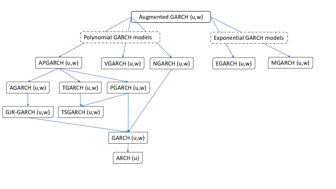
?figurename? 1: Schematic overview of the nesting of some augmented GARCH($p$,$q$) models.

?appendixname? B FCLT and CLTs used in the proofs

For the sake of completeness and to ease the understanding within the proofs, we cite here the multivariate FCLT as well as the two univariate CLTs to which we resort to.

B.1 Univariate FCLTs

Let us first state the FCLT for functionals of $\phi$-mixing processes.

Theorem 22 (Theorem 21.1 in [6]).

Suppose that the process $(Z_{n})_{n\in\mathbb{Z}}$ is $\phi$-mixing and its mixing rate $\phi_{n}$ satisfies $\sum\phi_{n}^{1/2}<\infty$. Then, for a given function $f$, consider the process $X_{n}=f(...,Z_{n-1},Z_{n},Z_{n+1},...),\leavevmode\nobreak\ n\in\mathbb{Z}$ and assume it to have mean 0 and finite variance. Suppose further, there exist random variables of the form $X_{ln}=f_{l}(Z_{n-l},...Z_{n},Z_{n+l})\text{\leavevmode\nobreak\ for\leavevmode\nobreak\ }f_{l}:\mathbb{R}^{2l+1}\mapsto\mathbb{R}$ such that $\sum_{l}E[\lvert X_{0}-X_{l0}\rvert^{2}]^{1/2}<\infty$. Then the series $\displaystyle\sigma^{2}=\operatorname{\mathbb{E}}[X_{0}]+2\sum_{k=1}^{\infty}\operatorname{\mathbb{E}}[X_{0}X_{k}]$  converges absolutely. If $\sigma^{2}>0$, then it holds:

$$\frac{1}{\sigma\sqrt{n}}S_{[nt]}(\omega)\overset{d}{\rightarrow}W,\quad\mbox{as}\;n\to\infty.$$

A corresponding FCLT for functionals of strong-mixing processes is the following:

Theorem 23 (Theorem 18.6.2 in [36]).

Suppose that the process $(Z_{n})_{n\in\mathbb{Z}}$ is strong mixing with mixing rate $\alpha(n)$. Then, for a given function $f$, consider the process $X_{n}=f(...,Z_{n-1},Z_{n},Z_{n+1},...),\leavevmode\nobreak\ n\in\mathbb{Z}$ and assume it to have mean 0 and finite variance. Suppose that, for some $\delta>0$, $\sum\alpha(n)^{\delta/(2+\delta)}<\infty$, $E[\lvert X_{0}\rvert^{2+\delta}]<\infty$ and $\sum\|X_{n}-\operatorname{\mathbb{E}}[X_{0}|\mathcal{F}_{-l}^{l}]\|_{(2+\delta)/(1+\delta)}<\infty$. Then the series $\displaystyle\sigma^{2}=\operatorname{\mathbb{E}}[X_{0}]+2\sum_{k=1}^{\infty}\operatorname{\mathbb{E}}[X_{0}X_{k}]$  converges.
If $\sigma^{2}>0$, then it holds:

$$\frac{1}{\sqrt{n}}S_{[n]}(\omega)\overset{d}{\rightarrow}\mathcal{N}(0,\sigma^{2}),\quad\mbox{as}\;n\to\infty.$$

B.2 Multivariate FCLTs

We state here the multivariate FCLT that we used in the proof of Theorem 3. It comes from [20] (Theorem 3.1)/ [17] (a multivariate version of Theorem 1.2), but adapted to our needs, as explained in Remark 25.

Theorem 24.

Consider a d-dimensional stationary random process $(u_{j},j\in\mathbb{Z})$ where each of the $d$ components is an $L_{2}$-NED process with constants $\nu(k)=O(k^{-\beta}),\beta>1/2$, with respect to the same (univariate) process $(V_{t})_{t\in\mathbb{Z}}$, which is either $\alpha$-mixing of order $\alpha(n)=O(n^{-\tilde{s}})$ for $\tilde{s}>s/(s-2)$, $s>2$, or $\phi$-mixing of order $\phi(n)=O(n^{-\tilde{s}})$ for $\tilde{s}>s/(2s-2)$, $s\geq 2$ - where, for this choice of $s$, it must hold that $\|u_{j,l}\|_{s}<\infty,\leavevmode\nobreak\ \forall j,l$. Further, assume that $\operatorname{Var}(\sum_{j=1}^{n}u_{j,l})/n:=\sigma_{n,l}/n\rightarrow\sigma_{l}^{2}>0$, $\forall l$, as $n\to\infty$.

Then, the series $\Gamma=\sum_{j\in\mathbb{Z}}\operatorname{Cov}(u_{0},u_{j})$ converges (coordinatewise) absolutely and a FCLT holds for $U_{n}:=\frac{1}{n}\sum_{j=1}^{n}u_{j}$:

$$\sqrt{n}tU_{[nt]}\overset{D_{d}[0,1]}{\rightarrow}W_{\Gamma}(t),\quad\mbox{as}\;n\to\infty,$$

where the convergence takes place in the d-dimensional Skorohod space $D_{d}[0,1]$ and $(W_{\Gamma}(t),t\in[0,1])$ is a d-dimensional Brownian motion with covariance matrix $\Gamma$, i.e. it has mean 0 and
$\operatorname{Cov}(W_{\Gamma}(u),W_{\Gamma}(t))=\min(u,t)\Gamma$.

Remark 25.

The conditions of our multivariate FCLT are similar to those stated in the univariate FCLT of [17] (see Theorem 1.2 therein). Their result is not restricted to stationary processes, but, for us, this is sufficient. This is why our conditions, by stationarity, will hold uniformly in $t$. It is also the reason why we do not need, in the definition of $L_{p}$-NED, a constant depending on the time $t$ of the process. Theorem 1.2 of [17] is a special case of Theorem 3.1 of [20], and this latter theorem has a multivariate equivalent presented in Theorem 3.2 in [20]. Combining these two ideas, we present in Theorem 24 a special case of Theorem 3.2. of [20].