Active microrheology in corrugated channels: comparison of thermal and colloidal baths

Abstract

HYPOTHESIS
The dynamics of colloidal suspension confined within porous materials strongly differs from that in the bulk. In particular, within porous materials, the presence of boundaries with complex shapes entangles the longitudinal and transverse degrees of freedom inducing a coupling between the transport of the suspension and the density inhomogeneities induced by the walls.
METHOD
Colloidal suspension confined within model porous media are characterized by means of active microrheology where a net force is applied on a single colloid (tracer particle) whose transport properties are then studied. The trajectories provided by active microrheology are exploited to determine the local transport coefficients. In order to asses the role of the colloid-colloid interactions we compare the case of a tracer embedded in a colloidal suspension to the case of a tracer suspended in an ideal bath.
FINDING
Our results show that the friction coefficient increases and the passage time distribution widens upon increasing the corrugation of the channel. These features are obtained for a tracer suspended in a (thermalized) colloidal bath as well as for the case of an ideal thermal bath. These results highlight the relevance of the confinement on the transport and show a mild dependence on the colloidal/thermal bath. Finally, we rationalize our numerical results with a semi-analytical model. Interestingly, the predictions of the model are quantitatively reliable for mild external forces, hence providing a reliable tool for predicting the transport across porous materials.

I Introduction

Microrheology has been introduced recently to study the microscopic diffusion of particles in complex environments Furst and Squires (2017). According to this technique, a tracer colloidal particle is introduced in the complex bath, and its diffusion is monitored, typically by microscopy. In passive microrheology, the tracer is allowed to diffuse and explore different regions Mason and Weitz (1995); Cicuta and Donald (2007); Wilson and Poon (2011), whereas in active microrheology, an external force is applied to the tracer, to make it travel long distances, allowing for the calculation of a microscopic friction coefficient and structural heterogeneities Habdas et al. (2004); Squires and Brady (2005); Gazuz et al. (2009); Puertas and Voigtmann (2014); Zia (2018). Theoretical models have been developed for bulk systems, relating the tracer dynamics with the properties of the bath, both for low densities Squires and Brady (2005); DePuit et al. (2011); Chu and Zia (2019), and dense systems Gazuz et al. (2009); Gruber et al. (2016); Su et al. (2017). Moreover, in the case of very strong pulling forces, non-linear response has been found for both bulk Bénichou et al. (2014) as well as for channels with constant sections Illien et al. (2014); Bénichou et al. (2016); Bénichou et al. (2018) . Microrheology has been applied to simple systems, where the models have been developed, but also to more complex systems beyond colloids, such as polymer or fiber solutions Gisler and Weitz (1999); Oppong et al. (2006), soaps Prasad and Weeks (2009), and particularly biological environments, such as mucus Weigand et al. (2017), or the interior of living cells Nishizawa et al. (2017).

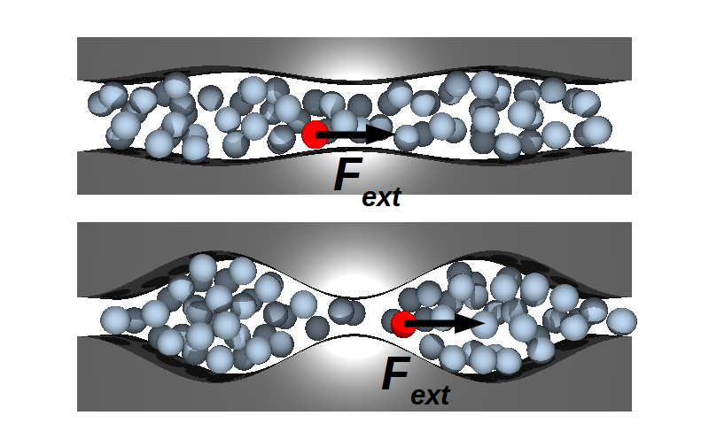
Figure 1: Snapshot of the systems with corrugation amplitudes of $A=0.51a$ (upper panel) and $A=1.62a$ (lower panel). In both cases, $L_{z}=L_{x}=6\,a$ and $L_{y}=40\,a$. The red particle is the tracer and the arrows indicate the direction of the force.

Accordingly, active microrheology seems a promising technique to study the transport of macromolecules, polymers or colloids suspended in complex fluids embedded in porous materials. Indeed, the spatial and time resolution probed by active microrheology can provide insight into the dependence of the transport on the local structural (density) modulations induced by the confining walls, and disentangle it from the effects of the complex fluid. The coupling of both effects can induce important modifications in the transport mechanism, such as non-isotropic diffusion Marconi et al. (2015); Puertas et al. (2018), that eventually may be exploited to tune the transport of the tracer.

The simplest model porous material is a one-dimensional channel as shown in Fig.1. When the confining walls are non-planar, the confinement induces structural (density) modulations, that affect also the transport properties along the principal channel direction. The solution of the general problem thus requires the solution of the three-dimensional diffusion equation, or the Fokker-Plank equation at the microscopic level, with the geometric constraints imposed by the channel. Alternatively, the problem can be studied effectively by the Fick-Jacobs approximation, that assumes that the equilibration in the transversal direction is much faster than the diffusion along the channel direction Jacobs (1967); Zwanzig (1992). This results again in a one-dimensional problem, where the external potentials (or confining walls) can be introduced. This description was improved by Zwanzig Zwanzig (1992), who introduced a space-dependent diffusion coefficient, and further developed in different works D. Reguera (2001); Kalinay and Percus (2006); Pineda et al. (2012); Berezhkovskii et al. (2015); Kalinay and Slanina (2018).

In this contribution, we exploit active microrheology to study the transport of colloids suspended in complex fluids embedded in porous materials. In particular, a colloidal suspension of hard particles containing a single tracer bead is confined in a varying-section channel. The tracer particle is subject to an external force, i.e. we implement the active microrheology protocol in a corrugated channel. We perform numerical simulations in which all particles have the same size and undergo Langevin dynamics. The average channel width is three particle diameters, and the narrowest point in the channel, channel neck, has been varied from five times the particle radius to three times. For small external forces, this implies a strong increase of the friction coefficient and mean first passage times, whereas for large forces, the effect of the corrugation amplitude is almost unnoticed.

In order to disentangle the dependence of the transport of the tracer on the properties of the complex fluid (i.e. the colloidal suspension) from the dependence on the shape of the channel, we compare our results against the case of a tracer suspended in an ideal thermal bath (Newtonian solvent) embedded in the same channel. The numerical results are also compared with a theoretical model that is based on the Fick-Jacobs approximation Jacobs (1967); Zwanzig (1992); D. Reguera (2001); Malgaretti et al. (2013). Within this model, the geometrical confinement is accounted for by an effective entropic force; the agreement of the model with the numerical data is quantitative for the isolated tracer and qualitative when the colloidal bath is included. This approach has provided insight for quite diverse confined systems including colloids Martens et al. (2011); Berezhkovskii et al. (2015), flow of (charged) fluids Martens et al. (2013); Malgaretti et al. (2014); Chinappi and Malgaretti (2018); Malgaretti et al. (2019a); Kalinay (2020), polymers Bianco and Malgaretti (2016); Malgaretti and Oshanin (2019); Carusela et al. (2021), rigid rods Malgaretti and Harting (2021), chemical reactions Ledesma-Durán et al. (2016), and pattern-forming systems Chacón-Acosta et al. (2020).

Our results show that active microrheology is a useful tool to characterize the transport of colloids suspended in confined complex fluids. In particular, with our technique we have been able to determine the local tracer position distribution and velocity. Moreover, the good match between our numerical results and the Fick-Jacobs model confirms the validity of the model to predict the local transport properties and to relate them to the macroscopic transport. Interestingly, our data show that some features, such as the tracer density profile or the Mean First Passage Time (MFPT) are robust with respect to the properties of the fluid the tracer is suspended in and their qualitative behavior can be predicted by our Fick-Jacobs model despite the bath is neglected.

II Numerical model

In the simulations, we consider a colloidal system of moderate density confined in a corrugated channel, with a tracer particle. All particles, including the tracer, have the same radius, $a$, and undergo Brownian motion. In addition to this random motion, an external force, parallel to the channel direction, acts on the tracer Puertas et al. (2018). The confining walls are defined by the corrugated surfaces:

$$h(y)=\pm\left(\frac{L_{z}}{2}-A\cos\frac{2\pi y}{\lambda}\right)$$ (1)

where $A$ and $\lambda$ are the corrugation amplitude and wavelength, respectively, and $L_{z}$ sets the mean separation of the walls, which we fix equal to $3$ particle diameters, i.e. $L_{z}=6a$. For later use we introduce the entropy barrier which for finite-size particles is defined as Malgaretti et al. (2016):

$$\Delta S=\ln\left[\frac{h_{max}-a}{h_{min}-a}\right]$$ (2)

with $h_{max}$ and $h_{min}$ the maximum and minimum channel widths, respectively. In all cases, the corrugation wavelength is $\lambda=20a$, and the volume fraction of the colloidal bath is $\phi=0.20$. The system has periodic boundary conditions in the $XY$ and $XZ$ planes. The snapshots in Fig. 1 show the systems with the lowest ($A=0.5\,\Delta S=0.33$) and highest ($A=1.2\,\Delta S=1.2$) corrugation amplitude.

In order to disentangle the effects of the bath and confinement, simulations without the colloidal bath have also been performed. In this case only the tracer confined between the walls is simulated, undergoing Brownian motion (due to the solvent, or thermal bath) and pulled by the external force.

Previous works of active microrheology in bulk or in channels have shown that the effective friction experienced by the tracer develops a plateau at low forces, what allows the definition of a linear regime Squires and Brady (2005); Carpen and Brady (2005); DePuit et al. (2011); Puertas and Voigtmann (2014); Puertas et al. (2018). Upon increasing the external force the effective friction decreases, i.e. the system experiences a so called, force-thinning regime. Finally, for large forces the friction reaches a second plateau, at a lower value than the low-force plateau. Therefore, we have selected three values of the external force, $\beta F_{ext}\lambda=10$, $100$ and $1000$, corresponding to the low-Péclet plateau, force thinning, and high-Péclet plateau, respectively. In particular cases, other values of the force have been simulated. Further details on the simulation method can be found in the Supplemental Material.

III Theoretical model

For a theoretical description of the system under consideration, we have used a model based on the Fick-Jacobs approximation of the transport properties of a channel, described in Ref.Malgaretti et al. (2016). All quantities in the theoretical model are intended in SI units. Briefly, after integration along the transverse direction, the time evolution of the distribution of the tracer position along the channel axis, $P(y,t)$, is given by:

$$\frac{\partial\rho_{y}(y,t)}{\partial t}=\frac{\partial}{\partial y}\left[\beta D(y)\rho_{y}(y,t)\frac{\partial{\cal A}(y)}{\partial y}+D(y)\frac{\partial\rho_{y}(y,t)}{\partial y}\right]$$ (3)

where $D(y)$ is the position-dependent diffusion coefficient and ${\cal A}(y)$ is the potential of mean force Marconi et al. (2015); Puertas et al. (2018). The steady-state solution of this equation reads:

$$\rho_{y}(y)=e^{-\beta\mathcal{A}(y)}\left[-J\int_{-\frac{\lambda}{2}}^{y}\dfrac{e^{\beta\mathcal{A}(y^{\prime})}}{D(y)}dy^{\prime}+\Pi\right]$$ (4)

with

$$\Pi =-J\dfrac{\displaystyle\int_{-\frac{\lambda}{2}}^{\frac{\lambda}{2}}\dfrac{e^{\beta\mathcal{A}(y^{\prime})}}{D(y^{\prime})}dy^{\prime}}{e^{-\beta\Delta\mathcal{A}}-1}=-J\Pi_{0}$$ (5)

$$J =-\left[\int_{-\frac{\lambda}{2}}^{\frac{\lambda}{2}}e^{-\beta\mathcal{A}(y)}\left[\int_{-\frac{\lambda}{2}}^{y}\dfrac{e^{\beta\mathcal{A}(y^{\prime})}}{D(y^{\prime})}dy^{\prime}+\Pi_{0}\right]dy\right]^{-1}$$ (6)

where $\Delta\mathcal{A}=\mathcal{A}(-\lambda/2)-\mathcal{A}(\lambda/2)$ and $\Pi$ and $J$ are determined by the periodic boundary condition and by the normalization

$$\int_{-\frac{\lambda}{2}}^{\frac{\lambda}{2}}P(y)dy=1$$ (7)

For the case of a single tracer suspended in an ideal gas, ${\cal A}(y)$ encodes only the confining forces and the external pulling force, $F_{ext}$:

$${\cal A}(y)=-k_{\text{B}}T\ln\left[\frac{h(y)}{h_{0}}\right]-F_{ext}y$$ (8)

whereas for interacting systems the functional form of ${\cal A}(y)$ is more involved Puertas et al. (2018). In the following we assume a constant diffusion coefficient along the channel, i.e.

$$D(y)=D_{0}$$ (9)

where $D_{0}$ is the bulk diffusion coefficient of the colloid.

We use Eq. (4) to determine the ratio between the probability of finding the tracer in the two halves of the channel $\rho_{L}/\rho_{R}$ which, in the limit of small forces, reduces to (see Suppl. Mat.):

$$\frac{\rho_{L}}{\rho_{R}}=1+\mathcal{H}\beta\Delta SF_{ext}\lambda\,.$$ (10)

where $\mathcal{H}$ is a prefactor whose value depends on the specific shape of the channel. We remark that in the expansion the product $\beta\Delta SF_{ext}\lambda$ naturally appears as the small parameter controlling the magnitude of higher order terms. This underlines that in the small-force regime $\Delta S$ and $\beta F_{ext}\lambda$ have a similar effect on the asymmetry in the distribution of the tracer.

III.1 Mean first passage time (MFPT)

A quantity that is often of interest in diffusion processes ranging from neuronal signaling to nuclear waste container Metzler et al. (2014) is the Mean First Passage Time (MFPT) i.e., the mean time that a particle takes to reach a certain location for the first time Redner (2001). Starting from Eq. (3), it is possible to derive an equation for the MFPT Gardiner (1994), $t_{1}(0)$, for a particle over a period of the channel $\lambda$ (see Suppl. Mat.):

$$t_{1}(0)=\frac{-\lambda^{2}}{D\left[(\beta F_{\text{ext}}\lambda)^{2}-(\beta\Delta{\cal F}\lambda)^{2}\right]^{2}}\times$$

$$\times\Bigg{[}e^{-\beta F_{\text{ext}}\lambda}((\beta\Delta{\cal F}\lambda)^{2}-(\beta F_{\text{ext}}\lambda)^{2})+$$ (11)

$$+\left(\beta F_{\text{ext}}\lambda\right)^{2}-\left(\beta F_{\text{ext}}\lambda\right)^{3}+3\left(\beta\Delta{\cal F}\lambda\right)^{2}+\beta F_{\text{ext}}\lambda\left(\beta\Delta{\cal F}\lambda\right)^{2}$$

$$+\dfrac{2\beta(F_{\text{ext}}\lambda-\Delta{\cal F}\lambda)\Delta{\cal F}\lambda-2e^{\beta\lambda\Delta{\cal F}}\Delta{\cal F}\lambda(F_{\text{ext}}\lambda+\Delta{\cal F}\lambda)}{e^{\frac{1}{2}\beta\lambda(F_{\text{ext}}+\Delta{\cal F})}}\Bigg{]}\,.$$

where we used the effective force

$${\cal F}(y)=\left\{\begin{array}[]{lll}{\cal F}_{1}=F_{ext}+\Delta\mathcal{F}&&y<0\\ {\cal F}_{2}=F_{ext}-\Delta\mathcal{F}&&y>0\end{array}\right.$$ (12)

derived from the free energy barrier

$$\Delta\mathcal{F}=-\frac{\mathcal{A}(0)-\mathcal{A}(\lambda/2)}{\lambda/2}.$$ (13)

Due to the complexity of Eq. (III.1), more insight can be obtained by focusing on some asymptotic behavior of $t_{1}(0)$. In the case of $F_{ext}=0$ and expressing the local force in the term of the free energy barrier $\Delta{\cal F}\lambda/2=-\Delta\mathcal{A}$ we obtain:

$$\lim_{F_{ext}\rightarrow 0}t_{1}(0)=\frac{8}{D\Delta{\cal F}^{2}}\sinh^{2}\left(\frac{\lambda\Delta{\cal F}}{4}\right)=\frac{\lambda^{2}}{D}\frac{\cosh\left(\beta\Delta\mathcal{A}\right)-1}{\left(\beta\Delta\mathcal{A}\right)^{2}}$$ (14)

that is in agreement with Ref.Malgaretti et al. (2016).
On the other hand, for large forces, $\beta F_{ext}\lambda\gg 1$, $t_{1}(0)$ reduces to

$$t_{1}(0)=\frac{\lambda^{2}}{D(\beta F_{ext}\lambda)}$$ (15)

Alternatively, for flat channels, $\Delta{\cal F}=0$, the MFPT reads:

$$t_{1}(0)=\frac{\lambda^{2}}{D(\beta F_{ext}\lambda)^{2}}\left[e^{-\beta F_{ext}\lambda}-1+\beta F_{ext}\lambda\right]$$ (16)

III.2 List of symbols and abbreviations

$a$	radius of the particles
$A(y)$	potential of mean force
$\beta$	inverse thermal energy
$D(y)$	position dependent diffusion coefficient
$D_{0}$	position independent diffusion coefficient
$F_{ext}$	external force acting on the tracer particle
	see Refs. Marconi et al. (2015); Puertas et al. (2018) and Eq.(8)
$\gamma_{eff}$	effective friction coefficient (see Eqs.(19),(20))
$\Delta\mathcal{F}$	effective force, see Eq.(12)
$J$	tracer particle flux
$h_{min,max}$	minimum, maximum channel amplitude
$\lambda$	channel period
$L_{x,z}$	channel thickness
$\rho_{y}(y)$	tracer particle probability distribution along $y$
$\rho_{L,R}$	probability of finding the tracer particle
	on the left (L) or roght (R) half of the channel
$P(\tau)$	probability distribution of first passage times
	(see Eq.(21))
$\Delta S$	see Eq.(2)
$t_{1}(0)$	MFPT from $y=0$ to $y=L$ (see Eq.(III.1))
$\tau_{p}$	decay time of the first passage time distribution
$\langle v_{y}(y)\rangle$	local longitudinal velocity (see Eq.(18))

IV Results

It is well known that interacting particles (or finite-size particles) form layers close to hard walls, due to the imbalance of the osmotic pressure Liétor-Santos et al. (2007); Sandomirski et al. (2011); Mansoori and Rice (2014); Kjellander (2019). When the wall is non-planar, this layering follows the shape of the walls, and in narrow corrugated channels it provokes a non-uniform density along the channel axis Puertas et al. (2018) (see Fig.S1). As expected, the density is symmetric with respect to the channel neck, and the maximum density is located in the neck. For the narrowest channel, the density increase in the neck is rather intense, that allows us to anticipate important effects on the transport properties.

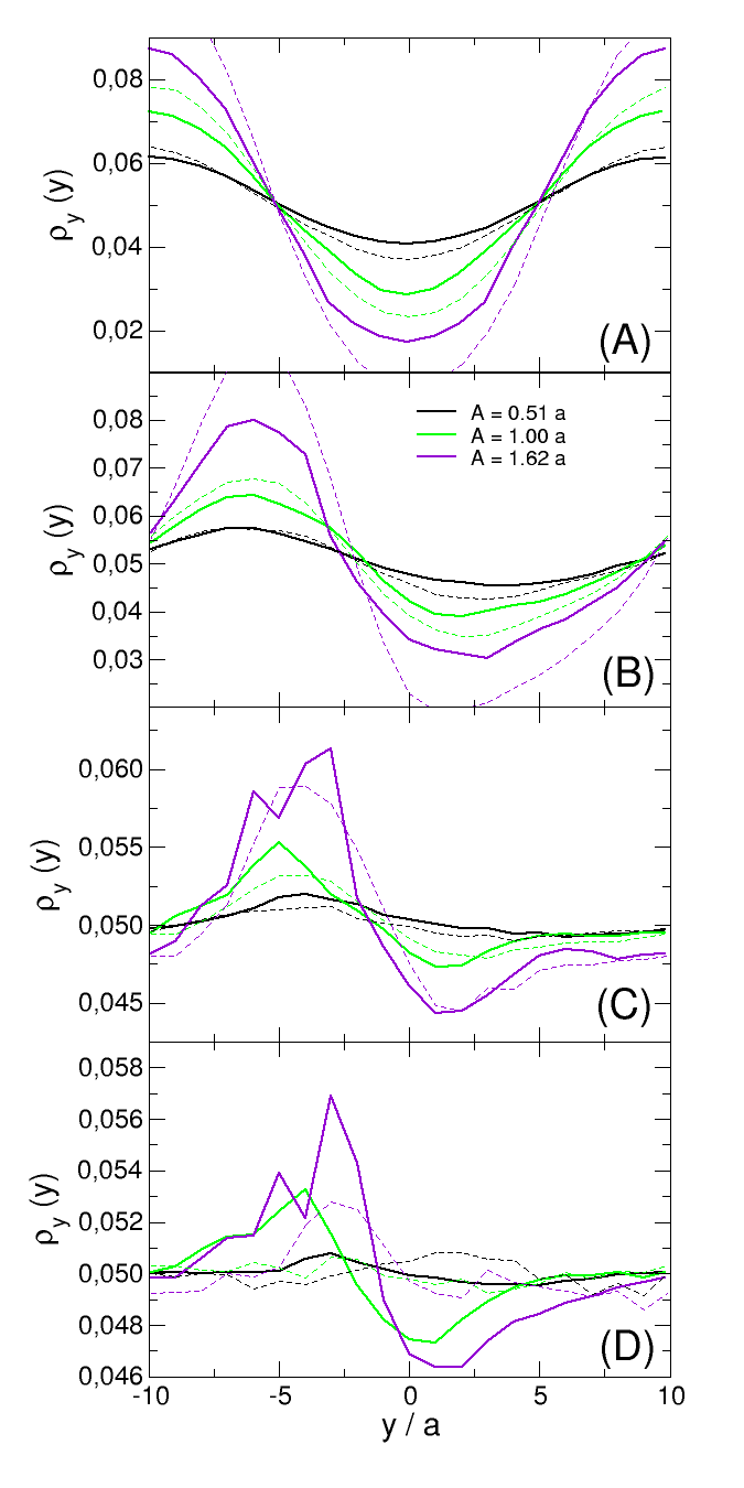
Figure 2: Integrated density, $\rho_{y}$, as function of the longitudinal position for different forces and corrugation amplitudes, as labeled. Solid lines represents the data for the colloidal bath, whereas dashed lines are for the thermal bath (solvent). From top to bottom: $\beta F_{ext}\lambda=0$, $10$, $100$, $1000$.

The density distribution reflects the tracer position distribution at force $\beta F_{ext}\lambda=0$. When a finite external force is applied, the symmetry around the neck is broken. In particular, such deviations from the equilibrium profile are those that eventually matter in determining the overall flux, Eq. (6), and hence they can be regarded as an indicator of the departure from equilibrium. Such deviations are more quantitatively observed calculating the density integrated in slabs perpendicular to the channel axis, namely, parallel to the $XZ$-plane:

$$\rho_{y}(y)\>=\>\frac{1}{P_{z}}\int_{\cal V}\rho(x,y,z)dzdx$$ (17)

where $\cal V$ is the slab volume, which we take of thickness $a$ along the longitudinal direction, and $P_{z}$ is a normalization constant introduced to guarantee that $\int_{-\lambda/2}^{\lambda/2}\rho_{y}(y)dy=1$. The integrated density $\rho_{y}$ is presented in Fig. 2 for different forces and channels. The most evident effect of the external force is that the symmetry with respect to the channel neck is broken: the tracer spends more time ”before” the neck than ”after” the neck (compare the diverse panels of Fig. 2). For large forces, the modulation of the density becomes less and less important (note that different scales are used in the different panels), and the tracer is more confined to the channel mid-plane. As shown in Fig. 2, the above mentioned behavior is robust and it holds for both colloidal and thermal bath (solvent). However, it is interesting to notice that, for smaller forces, the density of a tracer suspended in a thermal bath undergoes larger variations than the one for a tracer suspended in a colloidal bath whereas the opposite holds for larger forces.

For both the thermal and colloidal baths, the effect of the external force is first to shift the modulation of the integrated density, decreasing it only slightly. Larger forces decrease it more dramatically, with small changes in the maximum and minimum positions. Whereas the former trend breaks the symmetry between both sides of the channel, the latter recovers it by eliminating the density modulation.
The competition of these opposing effects is captured by the ratio of the integrated densities before and after the neck, $\rho_{L}/\rho_{R}$, presented in the top panel of Fig. 3. In all cases, the ratio $\rho_{L}/\rho_{R}$ displays a maximum around $\beta F_{ext}\lambda\approx 5-10$, and the ratio increases with the amplitude, $A$, of the corrugation. Interestingly, the position of the maximum coincides for both ideal and colloidal baths and is also in good quantitative agreement with the prediction of the Fick-Jacobs model.

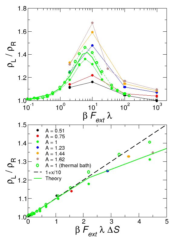
Figure 3: Top: Ratio of the integrated densities in the left and right of the channel neck. The color-code is reported in the legend. The solid green line is the theoretical prediction obtained by integrating Eq. (4) over the two halves of the channel. For $A=1a$, a finer grid of forces has been simulated, to locate the position of the maximum more accurately. Bottom: linear regime where the data collapse onto a straight line when plotted as function of $\beta F_{\text{ext}}\lambda\Delta S$. The solid green line is as in the upper panel, the solid yellow line is from Eq. (S$29$) that assumes a piece-wise linear effective free energy, whereas the dashed line is the fit of Eq. (10) to the data.

The bottom panel of Fig. 3 shows the density ratio for small forces as a function of $\beta F_{ext}\lambda\Delta S$ compared against the theoretical predictions, green solid line (see Fig.S2 for a quantitative estimation of the mismatch between the numerical data and the theoretical predictions). Interestingly, for small forces the data collapse on a straight line, as predicted by our simplified model, Eq. (10) with $\mathcal{H}=1/10$.

In order to analyze the tracer position distribution along the direction perpendicular to the force we can rely solely on numerical results since the theoretical model integrates out the transverse degrees of freedom. The variation of the tracer position distribution is studied in Fig. 4, where we focus on the plane $y=-\lambda/4=-5a$. The two extreme values of $A$, and the intermediate case are studied in the three force regimes, in addition to the unforced tracer (dashed lines). The density is normalized in all cases to give $\int_{V}\rho dV=1$, where $V$ is the volume of the channel from $y=-\lambda/2$ to $y=\lambda/2$.

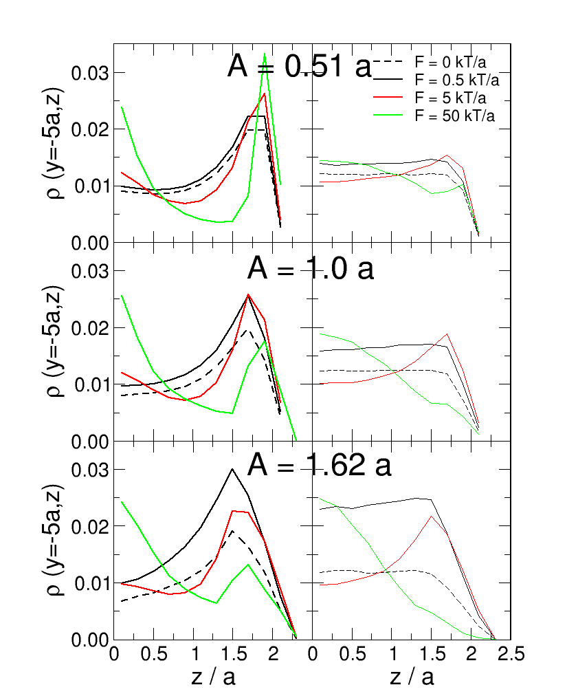
Figure 4: Density in the plane $y=-5\,a$ ($\lambda/4$ before the channel neck) for different corrugations and forces, as labeled, and the unforced tracer (dashed lines). Left panels are for the colloidal bath, right panels for the thermal bath (solvent).

As expected, in the absence of external forces the density distribution of a colloid suspended in a thermal bath (solvent) is homogeneous, whereas for a colloidal bath it shows accumulations at the walls. We remark that these accumulations are responsible for the onset of off-diagonal elements in the diffusion matrix in dense systems Marconi et al. (2015). In both baths, for small corrugations and forces, the distribution is only slightly modified, and it gets more affected upon increasing the value of the corrugation amplitude $A$, as anticipated by the shift of the maximum in the integrated densities in Fig. 2. More interestingly, the external force changes the density distribution qualitatively, increasing the tracer density at the channel mid-plane. The effect is more dramatic for the narrowest channel, where the maximum at $z=0$ surpasses the maximum at the wall. This indicates that the tracers are confined in the center of the channel due to the neck. The tracer distribution in other planes perpendicular to the force yield qualitatively the same conclusions.

IV.1 Tracer friction

We study next the dynamics of the tracer, focusing first on the tracer instantaneous velocity in the direction of the force, which we integrate in slabs perpendicular to the force:

$$\langle v_{y}(y)\rangle=\dfrac{\int_{\cal V}v_{y}(x,y,z)\rho(x,y,z)dxdz}{\int_{\cal V}\rho(x,y,z)dxdz}$$ (18)

where $\cal V$ corresponds to the same slabs as above. As naively expected, the velocity is lower than the average before the neck, and greater after it; the effect being more pronounced for larger channel modulations, for both baths (see Fig.(S2)). This explains the density variations along the channel, as the tracer spends more time before the neck than after it. Interestingly, while the velocity variation is symmetric for small forces, it becomes strongly asymmetric for larger ones, although the overall deviation from the average velocity decreases, corresponding to the force range where the density ratio $\rho_{L}/\rho_{R}$ decreases. Due to the collision with the bath particles, the tracer velocity is lower in the colloidal bath but the effects of the corrugation are qualitatively similar in both cases.

The tracer flux can be determined from the velocity as $J(y)=\langle v_{y}(y)\rangle\>\rho_{y}(y)$, which is independent of $y$, as expected for the stationary state. This determines the friction coefficient from the linear dependence of $J$ with $F_{ext}$

$$\bar{\rho}F=\gamma_{\text{eff}}J\,,$$ (19)

where $\bar{\rho}$ is the average density. Alternatively, the friction coefficient can be calculated from the mean tracer displacement for long times, $\delta y(t)$, and defining an average tracer velocity as $\bar{v}_{y}=\lim_{t\rightarrow\infty}\langle\delta y(t)\rangle/t$. The latter allows us to calculate the friction coefficient using the mean field relation

$$F_{ext}=\gamma_{\text{eff}}\bar{v}_{y}\,.$$ (20)

We remark that the two definition in Eq. (19) and Eq. (20) coincide. The top panel of Fig. 5 shows the results of $\gamma_{\text{eff}}$ as a function of the corrugation amplitude, for different forces and the two baths.

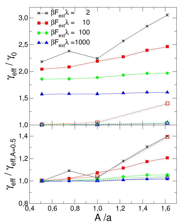
Figure 5: Top: Friction coefficient, $\gamma_{eff}$, as a function of the corrugation, for different external forces, as labeled. The results for the the colloidal bath are shown with filled symbols and solid lines whereas the thermal bath (solvent) is presented with open symbols and dashed lines. Bottom: same as top panel but for $\gamma_{eff}$ normalized by the value attained at $A/a=0.5$.

In all cases, the friction coefficient decreases with the force, corresponding to the microscopic equivalent of the shear thinning observed in viscoelastic fluids (the steps in the force are probably too high to detect any non-monotonic trend in the friction coefficient, as predicted by some theoretical worksIllien et al. (2014); Bénichou et al. (2016); Bénichou et al. (2018)). The agreement, within the statistical noise of the data, of the friction coefficient for $\beta F_{ext}\lambda=2$ and $\beta F_{ext}\lambda=10$ for small $A$ indicates that both forces are in the linear regime, while this has not been reached for large values of $A$. Interestingly, the increase of the friction coefficient at low forces is larger than at stronger pulling, resulting in more important thinning for strongly corrugated channels. This can be rationalized using the density profile perpendicular to the force (see Fig. 4), which indicates that the tracer is confined effectively to the central region of the channel for larger forces, thus passing through the neck irrespective of its width. This phenomenology is observed also for the thermal bath, where only for large corrugations the effective friction coefficient is significantly larger than the solvent friction coefficient. Interestingly, the lower panel of Fig.5 shows that the relative increase of $\gamma_{eff}$ of colloidal and thermal bath coincide at large forces whereas for weaker pulling the thermal bath shows an enhanced sensitivity to the geometry of the channel as compared to the colloidal bath. Hence colloid-colloid interactions reduce the sensitivity of the transport coefficient to the geometry. Such a feature can be of particular interest for polydisperse colloidal suspensions where the transport coefficients of different colloids may show a diverse sensitivity to the geometry of the channel.

Finally, we study also the transversal tracer velocity, integrated also in slabs of width $a$. The general effect of the corrugated channel is to push the tracer to the midplane before the neck and out of it after the neck, making particle diffusion anisotropic Marconi et al. (2015) for both baths. This effect is enhanced for large corrugations and forces (see Fig.S3 where a negative velocity indicates ”to-the-midplane”, whereas a positive velocity is ”out-of-the-midplane”). For small forces, the data for different corrugation amplitudes collapse onto a master curve (within the statistical noise), when the velocity is rescaled with the force, indicating a linear regime also in the transversal velocity. For larger forces, the confining before the neck is more intense for strong corrugations, as noted by the deep minimum of $v_{z}$ for large $A$, more intense for the thermal bath. These results are consistent with the maximum tracer density in the midplane (Fig. 4) and the concomitant independence of the friction with the corrugation amplitude (Fig. 5) for large forces, and ultimately with the diffusion anisotropy observed in non-planar channels, irrespective of the presence of the colloidal bath.

IV.2 Mean First Passage times

We finally study the first passage times, $\tau$, of the forced tracer. In particular we focus on the Mean First Passage Time (MFPT), $t_{1}=\langle\tau\rangle$, extracted from the passage time distributions (see suppl. mat.). The MFPT is plotted in Fig. 6 for all forces and three corrugation amplitudes, as well as the results of the isolated tracer, which can be accurately described by the theoretical model. As expected, the presence of the colloidal bath increases the MFPT due to the increase in the effective friction, but the overall dependence of $t_{1}$ on the force is unaffected (compare the open and closed circles in the figure). The graph also shows that for small forces the MFPT depends also on the corrugation amplitude, while it becomes independent for large forces. This result is in agreement with the simulations of the single particle and the theoretical model, as shown by the limits for small and large force, Eqs. (14) and (15). Also, the decay of the MFPT for the large forces as $\propto 1/F_{ext}$ is correctly predicted, although the prefactor is modified by the colloidal bath.

The inset of Fig.6 shows the deviation of $t_{1}$ from the decay $\propto 1/F_{ext}$ by plotting the product $t_{1}F_{ext}$. Interestingly, tracers in a colloidal bath show a remarkable difference as compared to their counterparts in a purely ideal bath. Such a difference persists for a few decades and can be exploited to characterize the properties of the colloidal bath from the MFPT of the tracer.

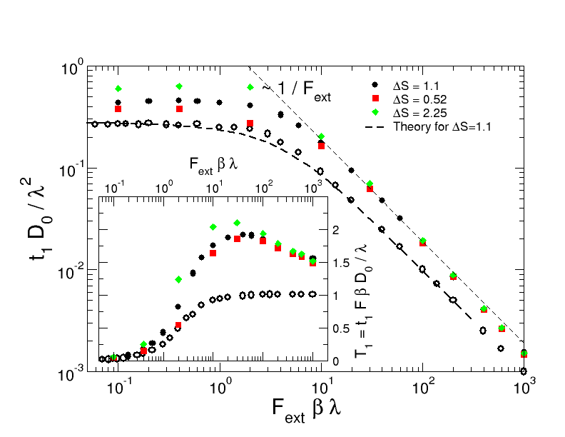
Figure 6: Mean first passage times as a function of the force for different corrugations, as labeled. The open symbols show the results for the isolated tracer.

The full distributions of first passage times $T=\tau\beta F_{ext}D_{0}/\lambda$ are presented in Fig.S4 for different forces and corrugation parameters in the presence of the colloidal bath. All distributions are strongly asymmetric, with an exponential decay for large times. Comparing the passage time distributions for different forces, one notices that the decay for large times is strongly reduced for larger forces, but the maximum is almost constant when corrected with the force, as expected from our model for large forces (see eq. 15). Similar tails in the distribution of passage times are also present in the case of an isolated Brownian tracer (not shown). A salient feature of the distribution of passage times is its decay for large times. We have fitted this decay with an exponential form (see dashed lines in Fig.S4),

$$P(\tau)\sim\exp\left\{-\tau/\tau_{p}\right\},$$ (21)

to extract its characteristic time scale $\tau_{p}$. This is presented in Fig. 7 for different forces and corrugations. As for the case of the MFTP, $\tau_{p}$ depends on the corrugation amplitude only for small forces, while it is constant for large forcings. The inset in the figure shows the evolution of $\tau_{p}$ with the force for a corrugation amplitude of $A=1.0a$, comparing the tracer in the bath with an isolated tracer. Similar to the MFPT, $\tau_{p}$ is constant for small forces and decreases for large forces faster than $1/F$ in both cases. Again, the effect of the bath is to increase the time scales keeping the dependence on the corrugation amplitude and on the external force.

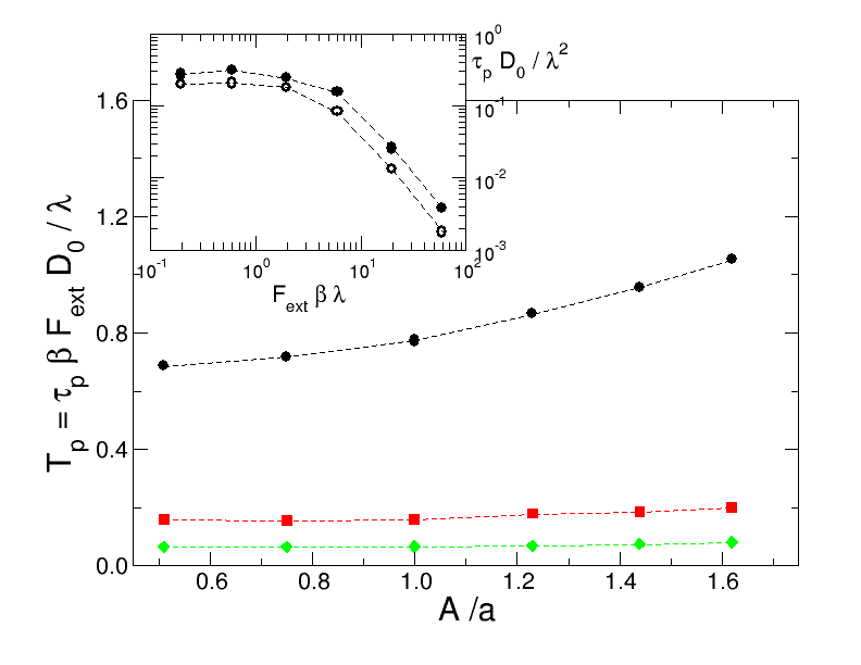
Figure 7: Characteristic time as a function of the corrugation amplitude, for different forces, as labeled. The inset shows $\tau_{p}$ as a function of the force for the isolated tracer (open circles) and in the colloidal bath (solid circles).

V Conclusions

Microrheology has been applied to simple systems, where the models have been developed, and also to more complex systems beyond colloids, such as polymer or fiber solutions Gisler and Weitz (1999); Oppong et al. (2006), soaps Prasad and Weeks (2009), and particularly biological environments, such as mucus Weigand et al. (2017), or the interior of living cells Nishizawa et al. (2017).

In this work, we present simulations and a theoretical model of active microrheology in corrugated channels, studying the effect of the corrugation amplitude: a tracer particle is pulled with a constant force through a colloidal bath confined in the channel. The model is based on the Fick-Jacobs approximation Jacobs (1967); Zwanzig (1992); D. Reguera (2001); Kalinay and Percus (2006); Kalinay and Slanina (2018) for an isolated tracer in a corrugated channel, and it is validated by simulations without the colloidal bath (only the solvent, as a thermal bath, is considered). The results of the simulations with the colloidal bath follow the same trends of the isolated tracer, although quantitative differences are noticed.

In particular, the simulation results show that upon increasing the corrugation amplitude, the tracer accumulates at the channel neck: the position distribution peaks, the velocity parallel to the force decreases, and the resulting friction coefficient increases. As a result, the distribution of passage times becomes more heterogeneous for narrower bottlenecks. On the other hand, for strong forces, the tracer is confined effectively to the center of the channel as shown by the tracer position distribution and the transversal velocity. Thus, the friction coefficient decreases Squires and Brady (2005); Carpen and Brady (2005); DePuit et al. (2011); Puertas and Voigtmann (2014); Puertas et al. (2018) and the passage time distribution narrows, with the force thinning effect being more important for large corrugations. These general trends are obtained for the colloidal bath but also for the thermal bath, indicating that the origin of this phenomenology is the confinement, and the colloidal bath modifies it only quantitatively. Strong effects are noticed, nevertheless, in the effective friction, and in particular the force thinning.

The comparison with the model is performed quantitatively by studying the ratio of the densities before and after the neck, and the mean first passage times. The former grows linearly for small forces, with a slope proportional to the corrugation parameter $\Delta S$, in agreement with the model. For larger forces, the ratio displays a maximum whose position depends only slightly on $\Delta S$. The mean first passage time shows a plateau for small forces, and decreases as the inverse of the force, also in agreement with the the model. The effect of the bath is again merely quantitative for these two parameters.

The good agreement between the colloidal and thermal bath is the cornerstone that proves the reliability of the semi-analytical model. Indeed, the model is derived under the assumption of an ideal bath and hence it can work only when colloid-colloid interactions are disregardable. Interestingly, our work shows that the regime of reliability of the semi-analytical model extends up to moderate densities, $\phi=0.2$, of the colloidal bath. This implies that the model we propose can provide quantitatively reliable predictions about the transport of colloidal suspensions across porous media. Such a quantitatively reliable and simple model can be exploited in several biological and technological applications, spanning from mucus Weigand et al. (2017), or the interior of living cells Nishizawa et al. (2017) to oil recovery Gravelle et al. (2011); Foroozesh and Kumar (2020); Zhang et al. (2020); Bizmark et al. (2020) and gas production where the colloidal particle concentration can be quire low, $\phi\simeq 0.05$, see Refs. Gravelle et al. (2011); Bizmark et al. (2020).
Moreover, our findings provide a solid starting point for exploring the more complex transport regimes that may occur at higher densities Gazuz et al. (2009); Gruber et al. (2016); Su et al. (2017). Indeed, theoretical models have predicted the onset of non-linear response in driven dense systems Bénichou et al. (2013). In addition, we foresee possible extensions of the model, for example to account for unsteady flows or time-dependent pressure drops Fourar et al. (2004).
Finally, in many circumstances like transport in narrow channels Malgaretti et al. (2019b), polymer translocation Muthukumar (2011), or any instance that triggers an irreversible cascade of events, the stationary flux is not the quantity of interest, rather the first passage time Metzler et al. (2014) is the crucial quantity. Our comparison shows that such quantity can be reliably predicted even in the presence of particle-particle interactions and correlations, hence extending previous ones Malgaretti et al. (2016) that did not account for interactions among particles.

Simulations details

The equation of motion for all particles is:

$$m\ddot{\vec{r}}_{j}=-\gamma_{0}\dot{\vec{r}}_{j}+\vec{\eta}_{j}(t)+\sum_{i\neq j}\vec{F}_{ij}+\vec{F}_{wall}+\delta_{j1}\vec{F}_{ext},$$ (22)

where the forces acting on particle $j$ are the friction with the solvent, $\gamma_{0}\dot{\vec{r}}_{j}$, proportional to the friction coefficient $\gamma_{0}$ and the particle velocity $\dot{\vec{r}}_{j}$, the random force $\vec{\eta}_{j}(t)$, which verifies the fluctuation-dissipation theorem, and the interaction forces with other particles ($\vec{F}_{ij}$) and the walls ($\vec{F}_{wall}$). An additional external force, $\vec{F}_{ext}$, pulls the tracer, labelled $j=1$; this force is constant, and acts in the $y$-direction, $\vec{F}_{ext}=F_{ext}\vec{e}_{y}$.

The interparticle forces between particles and with the walls derive from the continuous potentials:

$$V(r)=k_{\text{B}}T\left(\frac{r}{2a}\right)^{-36}\hskip 14.22636pt\mbox{and}\hskip 14.22636ptV_{w}(d)=k_{\text{B}}T\left(\frac{d}{a}\right)^{-36}$$ (23)

respectively, where $r$ is the center to center distance between particles and $d$ is the minimum distance from the particle center to the wall.

The confining walls are defined by the corrugated surfaces:

$$z=\pm\left(\frac{L_{z}}{2}-A\cos\frac{2\pi y}{\lambda}\right)$$ (24)

where $A$ and $\lambda$ are the corrugation amplitude and wavelength, respectively, and $L_{z}$ sets the mean separation of the walls, which we set equal to $3$ particle diameters, i.e. $L_{z}=6a$.

In this work we have considered channels with different amplitudes, as shown in Table 1. The entropy barrier is also given, which for finite-size particles is defined as Malgaretti et al. (2016):

$$\Delta S=\ln\left[\frac{h_{max}-a}{h_{min}-a}\right]$$ (25)

$A/a$	$\hskip 14.22636pt\Delta S\hskip 14.22636pt$
0.51	0.522
0.75	0.788
1.0	1.099
1.23	1.434
1.44	1.815
1.62	2.254

Table 1: Values of the corrugation amplitude, $A$, and entropy barrier, $\Delta S$, used in this work.

with $h_{max}$ and $h_{min}$ the maximum and minimum channel widths, respectively. In all cases, the corrugation wavelength is $\lambda=20a$, and the volume fraction of the colloidal bath is $\phi=0.20$. The simulation box has dimensions $L_{x}\times L_{y}\times L_{z}$, with $L_{x}=L_{z}=6a$ and $L_{y}=2\lambda$, resulting in $69$ particles, including the tracer. The system has periodic boundary conditions in the $XY$ and $XZ$ planes. The snapshots in Fig.1 of the main text show the systems with the lowest and highest $\Delta S$ (upper and lower panels, respectively).

The system is equilibrated without external force and at time $t=0$, the external force is switched on. The tracer trajectory, as well as the bath average properties, are recorded. The first passage time is estimated from the time of two subsequent passages of the tracer by the neck from left to right.

In the simulations, the length unit is the particle radius, $a$, the particle mass, $m$, is set to unit,and energy is measured in units of $k_{\text{B}}T$. The friction coefficient with the solvent is set to $\gamma_{0}=10\sqrt{k_{\text{B}}Tm}/a$, which corresponds to a Brownian time (the time required to diffuse a distance equal to $a$) $\tau_{B}=\gamma_{0}/6k_{\text{B}}T=1.67a\sqrt{m/k_{\text{B}}T}$. The equations of motion (22) are integrated with a Heun algorithm Ascher (1998) with a time step of $\delta t=0.0005a\sqrt{m/k_{\text{B}}T}$.

Derivation of Eq.(10) of the main text

At steady state the density profile reads:

$$\rho(y)=e^{-\beta A(y)}\left[-\frac{J}{D}\int_{-\frac{\lambda}{2}}^{y}e^{\beta A(z)}dz+\Pi\right]$$ (26)

with

$$\beta A(y) =\beta A_{0}(y)-\beta fy$$ (27)

$$\Pi =-\frac{J}{D}\frac{\int_{-\frac{\lambda}{2}}^{\frac{\lambda}{2}}e^{\beta A(z)}dz}{e^{-\beta(A(-\lambda/2)-A(\lambda/2))}-1}=-\frac{J}{D}\Pi_{0}$$ (28)

$$\frac{J}{D} =-\left[\int_{-\frac{\lambda}{2}}^{\frac{\lambda}{2}}e^{-\beta A(y)}\left[\int_{-\frac{\lambda}{2}}^{y}e^{\beta A(z)}dz+\Pi_{0}\right]dy\right]^{-1}$$ (29)

Recalling that $\beta A_{0}(y)=\beta A_{0}(y+L)$, for small forces we have:

$$\Pi_{0} \simeq -\frac{\int_{-\frac{\lambda}{2}}^{\frac{\lambda}{2}}e^{\beta A(z)}dz}{\beta f\lambda-\frac{1}{2}\left(\beta f\lambda\right)^{2}}$$ (30)

$$J \simeq \frac{\beta Df}{\lambda}\frac{1}{Z}$$ (31)

$$Z = \frac{1}{\lambda}\int_{-\frac{\lambda}{2}}^{\frac{\lambda}{2}}e^{-\beta A_{0}(z)}dz\frac{1}{\lambda}\int_{-\frac{\lambda}{2}}^{\frac{\lambda}{2}}e^{\beta A_{0}(z)}dz$$ (32)

Note that due to symmetry reasons we have that $J$ has no contribution proportional to $f^{2}$. At linear order in $f$ we have:

$$\rho(y)\simeq \frac{1}{Z}e^{-\beta A_{0}(y)}\left(1+\beta fy\right)\frac{1}{\lambda}\left[-\beta f\int_{-\frac{\lambda}{2}}^{y}e^{\beta A_{0}(z)}(1-\beta fz)dz\right.$$

$$\left.+\left(1+\beta f\frac{\lambda}{2}\right)\frac{1}{\lambda}\int_{-\frac{\lambda}{2}}^{\frac{\lambda}{2}}e^{\beta A_{0}(z)}(1-\beta fz)dz\right]$$ (33)

by collecting terms we obtain:

$$\rho(y)\simeq \frac{1}{Z}e^{-\beta A_{0}(y)}\frac{1}{\lambda}\left[-\beta f\int_{-\frac{\lambda}{2}}^{y}e^{\beta A_{0}(z)}dz\right.$$

$$\left.+\frac{1}{\lambda}(1+\beta fy+\beta f\frac{\lambda}{2})\int_{-\frac{\lambda}{2}}^{\frac{\lambda}{2}}e^{\beta A_{0}(z)}dz-\frac{1}{\lambda}\int_{-\frac{\lambda}{2}}^{\frac{\lambda}{2}}\beta fze^{\beta A_{0}(z)}dz\right]$$ (34)

Moreover, assuming that

$$\beta A_{0}(y)=\begin{cases}-2\Delta S\frac{y}{\lambda}&y<0\\ 2\Delta S\frac{y}{\lambda}&y>0\end{cases}$$ (35)

Hence we get:

$$\int_{-\frac{\lambda}{2}}^{\frac{\lambda}{2}}e^{\beta A_{0}(z)}dz =\frac{\lambda}{\Delta S}\left[e^{\Delta S}-1\right]$$ (36)

$$\int_{-\frac{\lambda}{2}}^{\frac{\lambda}{2}}\beta fze^{\beta A_{0}(z)}dz =0$$ (37)

$$\int_{-\frac{\lambda}{2}}^{y}e^{\beta A_{0}(z)}dz =\Gamma(y)=\begin{cases}\frac{\lambda}{2\Delta S}\left(e^{\Delta S}-e^{-2\Delta S\frac{y}{\lambda}}\right)&y<0\\ \frac{\lambda}{2\Delta S}\left(e^{\Delta S}-2+e^{2\Delta S\frac{y}{\lambda}}\right)&y>0\end{cases}$$ (38)

$$Z =\frac{1}{\Delta S}\left[e^{\Delta S}-1\right]\frac{1}{\Delta S}\left[1-e^{-\Delta S}\right]=\frac{2}{\Delta S^{2}}\left(\cosh\Delta S-1\right)$$ (39)

that leads

$$\rho(y)\simeq\frac{1}{Z}\begin{cases}e^{2\Delta S\frac{y}{\lambda}}\frac{1}{\lambda}\left[-\beta f\frac{\lambda}{2\Delta S}\left(e^{\Delta S}-e^{-2\Delta S\frac{y}{\lambda}}\right)+\frac{1+\beta fy+\beta f\frac{\lambda}{2}}{\Delta S}\left(e^{\Delta S}-1\right)\right]&y<0\\ e^{-2\Delta S\frac{y}{\lambda}}\frac{1}{\lambda}\left[-\beta f\frac{\lambda}{2\Delta S}\left(e^{\Delta S}-2+e^{2\Delta S\frac{y}{\lambda}}\right)+\frac{1+\beta fy+\beta f\frac{\lambda}{2}}{\Delta S}\left(e^{\Delta S}-1\right)\right]&y>0\end{cases}$$ (40)

Expanding for small $\Delta S$ we get:

$$\Gamma(y) \simeq\begin{cases}\Gamma_{-}(y)=\frac{1}{2}+\frac{y}{\lambda}+\Delta S\left[\frac{1}{4}-\left(\frac{y}{\lambda}\right)^{2}\right]+\Delta S^{2}\left[\frac{1}{12}+\frac{2}{3}\left(\frac{y}{\lambda}\right)^{3}\right]y<0\\ \Gamma_{+}(y)=\frac{1}{2}+\frac{y}{\lambda}+\Delta S\left[\frac{1}{4}+\left(\frac{y}{\lambda}\right)^{2}\right]+\Delta S^{2}\left[\frac{1}{12}+\frac{2}{3}\left(\frac{y}{\lambda}\right)^{3}\right]y>0\end{cases}$$ (41)

$$\frac{1+\beta fy}{\Delta S}\left(e^{\Delta S}-1\right) \simeq\left(1+\beta fy\right)\left(1+\frac{\Delta S}{2}+\frac{\Delta S^{2}}{6}\right)$$ (42)

$$\frac{1}{Z} \simeq 1-\frac{1}{12}\Delta S^{2}$$ (43)

and the we get:

$$\rho(y)\simeq\begin{cases}\frac{1}{\lambda}\left(1+2\Delta S\frac{y}{\lambda}+2\left(\Delta S\frac{y}{\lambda}\right)^{2}\right)\cdot\\ \cdot\left[-\beta f\lambda\Gamma_{-}(y)+\left(1+\beta fy+\beta f\frac{\lambda}{2}\right)\left(1+\frac{\Delta S}{2}+\frac{\Delta S^{2}}{6}\right)\right]\left(1-\frac{\Delta S^{2}}{12}\right)y<0\\ \frac{1}{\lambda}\left(1-2\Delta S\frac{y}{\lambda}+2\left(\Delta S\frac{y}{\lambda}\right)^{2}\right)\cdot\\ \cdot\left[-\beta f\lambda\Gamma_{+}(y)+\left(1+\beta fy+\beta f\frac{\lambda}{2}\right)\left(1+\frac{\Delta S}{2}+\frac{\Delta S^{2}}{6}\right)\right]\left(1-\frac{\Delta S^{2}}{12}\right)y>0\end{cases}$$ (44)

that can be simplified to

$$\rho(y)\simeq\frac{1}{\lambda}\begin{cases}1+\left[\frac{1}{2}+2\frac{y}{\lambda}+\beta f\lambda\left(\frac{1}{2}\frac{y}{\lambda}+\left(\frac{y}{\lambda}\right)^{2}\right)\right]\Delta S+\\ +\frac{1}{12}\left[1+12\frac{y}{\lambda}+24\left(\frac{y}{\lambda}\right)^{2}+\beta f\lambda\left(2\frac{y}{\lambda}+12\left(\frac{y}{\lambda}\right)^{2}+16\left(\frac{y}{\lambda}\right)^{3}\right)\right]\Delta S^{2}&y<0\\ 1+\left[\frac{1}{2}-2\frac{y}{\lambda}+\beta f\lambda\left(\frac{1}{2}\frac{y}{\lambda}-\left(\frac{y}{\lambda}\right)^{2}\right)\right]\Delta S+\\ +\frac{1}{12}\left[1-12\frac{y}{\lambda}+24\left(\frac{y}{\lambda}\right)^{2}+\beta f\lambda\left(2\frac{y}{\lambda}-12\left(\frac{y}{\lambda}\right)^{2}+16\left(\frac{y}{\lambda}\right)^{3}\right)\right]\Delta S^{2}&y>0\end{cases}$$ (45)

Defining

$$\rho_{\lambda} = \int_{-\frac{\lambda}{2}}^{0}\rho(y)dy$$ (46)

$$\rho_{R} = \int_{0}^{\frac{\lambda}{2}}\rho(y)dy$$ (47)

we have:

$$\rho_{\lambda} = \frac{1}{2}-\frac{1}{48}\beta f\lambda\Delta S+\mathcal{O}(\Delta S^{3})$$ (48)

$$\rho_{R} = \frac{1}{2}+\frac{1}{48}\beta f\lambda\Delta S+\mathcal{O}(\Delta S^{3})$$ (49)

for small values of $f$ we can expand the ratio:

$$\frac{\rho_{\lambda}}{\rho_{R}}=1-\frac{1}{12}\beta f\lambda\Delta S$$ (50)

We remark that the $1/12$ prefactor is due to the linear approximation of the free energy, Eq. 35. For other free energy profile with the same free-energy barrier $\Delta S$ we expect to have:

$$\frac{\rho_{\lambda}}{\rho_{R}}=1-\mathcal{H}\beta f\lambda\Delta S$$ (51)

Derivation of Eq.11 of the main text

Starting from Eq. (3) of the main text, it is possible to derive an equation for the MFPT Gardiner (1994), $t(y)$, for a particle over a period:

$$-\beta D\left(\partial_{y}{\cal A}(y)\right)\partial_{y}t(y)+D\partial_{y}^{2}t(y) =-1$$ (52)

$$\partial_{y}t(y)|_{-\lambda/2} =0$$ (53)

$$t(y)|_{\lambda/2} =0$$ (54)

In order to gain analytical insight in solving Eq. (52), it is more convenient Malgaretti et al. (2016) to approximate the effective potential as piece-wise linear:

$${\cal A}(y)=\left\{\begin{array}[]{lll}-F_{ext}y+\Delta\mathcal{A}\frac{y}{\lambda/2}&\hskip 28.45274pt-\frac{\lambda}{2}<y<0\\ -F_{ext}y-\Delta\mathcal{A}\frac{y}{\lambda/2}&\hskip 37.55785pt0\leq y<\frac{\lambda}{2}\end{array}\right.$$ (55)

where $\Delta\mathcal{A}=\mathcal{A}(0)-\mathcal{A}(-\lambda/2)$. Accordingly we can define the piece-wise linear force:

$${\cal F}(y)=\left\{\begin{array}[]{lll}{\cal F}_{1}=F_{ext}+\Delta\mathcal{F}&&y<0\\ {\cal F}_{2}=F_{ext}-\Delta\mathcal{F}&&y>0\end{array}\right.$$ (56)

with $\Delta\mathcal{F}=-\frac{\Delta\mathcal{A}}{\lambda/2}$. First, we rewrite the MFPT equation, Eq. (52) as

$$\beta D{\cal F}(y)\partial_{y}t(y)+D\partial_{y}^{2}t(y) =-1$$ (57)

Using the auxiliary variable $\partial_{y}t(y)=T(y)$ the last equations read:

$$\beta D{\cal F}(y)T(y)+D\partial_{y}T(y) =-1$$ (58)

$$T(y)|_{-\lambda/2} =0$$ (59)

Then we split Eq. (58) into two equations:

$$\begin{cases}\beta D{\cal F}_{1}T_{1}(y)+D\partial_{y}T_{1}(y)=-1&x<0\\ \beta D{\cal F}_{2}T_{2}(y)+D\partial_{y}T_{2}(y)=-1&x>0\end{cases}$$ (60)

whose solutions read:

$$T_{1}(y) = e^{-\beta{\cal F}_{1}y}\left[-\frac{1}{D}\int_{-\frac{\lambda}{2}}^{y}e^{\beta{\cal F}_{1}y^{\prime}}dy^{\prime}+\Pi_{1}\right]$$ (61)

$$T_{2}(y) = e^{-\beta{\cal F}_{2}y}\left[-\frac{1}{D}\int_{0}^{y}e^{\beta{\cal F}_{2}y^{\prime}}dy^{\prime}+\Pi_{2}\right]$$ (62)

and finally

$$t_{1}(y) =\int_{-\frac{\lambda}{2}}^{y}T_{1}(y^{\prime})dy^{\prime}+\Lambda_{1},\, \text{for}\,x<0$$ (63)

$$t_{2}(y) =\int_{0}^{y}T_{2}(y^{\prime})dy^{\prime}+\Lambda_{2},\, \text{for}\,x>0$$ (64)

with the continuity conditions:

$$t_{1}(0) = t_{2}(0)$$ (65)

$$T_{1}(0) = T_{2}(0)$$ (66)

Due to the B.C. (Eqs.53, 54) we have

$$\Pi_{1} =0$$ (67)

$$\Lambda_{2} =-\int_{0}^{\frac{\lambda}{2}}T_{2}(x)dx$$ (68)

Imposing the continuity leads to

$$\Pi_{2} = T_{1}(0)$$

$$\Lambda_{1} = -\left[\int_{-\frac{\lambda}{2}}^{0}T_{1}(y)dy+\int_{0}^{\frac{\lambda}{2}}T_{2}(y)dy\right]$$

The quantity we are interested in is $t_{1}(0)$:

$$t_{1}(0)= -\frac{\lambda^{2}}{D\left[(\beta F_{\text{ext}}\lambda)^{2}-(\beta\Delta{\cal F}\lambda)^{2}\right]^{2}}\left[e^{-\beta F_{\text{ext}}\lambda}((\beta\Delta{\cal F}\lambda)^{2}-(\beta F_{\text{ext}}\lambda)^{2})\right.$$

$$+\left(\beta F_{\text{ext}}\lambda\right)^{2}-\left(\beta F_{\text{ext}}\lambda\right)^{3}+3\left(\beta\Delta{\cal F}\lambda\right)^{2}+\beta F_{\text{ext}}\lambda\left(\beta\Delta{\cal F}\lambda\right)^{2}$$

$$\left.+e^{-\frac{1}{2}\beta\lambda(F_{\text{ext}}+\Delta{\cal F})}\left(2\beta(F_{\text{ext}}\lambda-\Delta{\cal F}\lambda)\Delta{\cal F}\lambda-2e^{\beta\lambda\Delta{\cal F}}\Delta{\cal F}\lambda(F_{\text{ext}}\lambda+\Delta{\cal F}\lambda)\right)\right]$$ (69)

Density of colloidal particles

Particle density in our system of quasi-hard spheres at volume fraction $\phi=0.20$, without external forces, for the two extreme corrugation amplitudes.

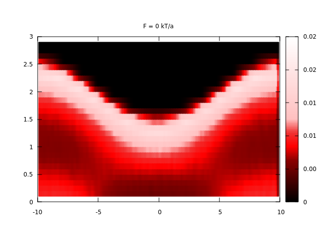
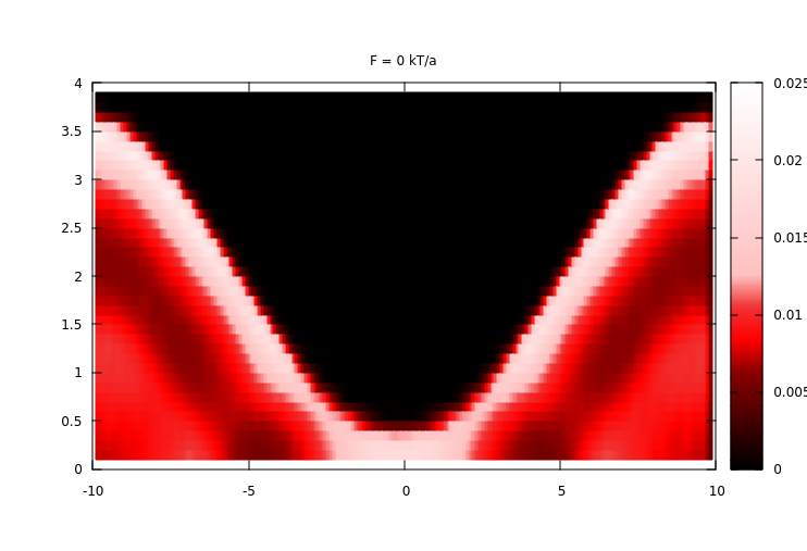
Figure 8: Equilibrium ($\beta F\lambda=0$), probability density of the tracer for $A=0.51a$ (upper panel) and $A=1.62a$ (lower panel). In both cases, $L_{z}=L_{x}=6\,a$ and $L_{y}=2\lambda=40\,a$.

Theoretical/numerical comparison

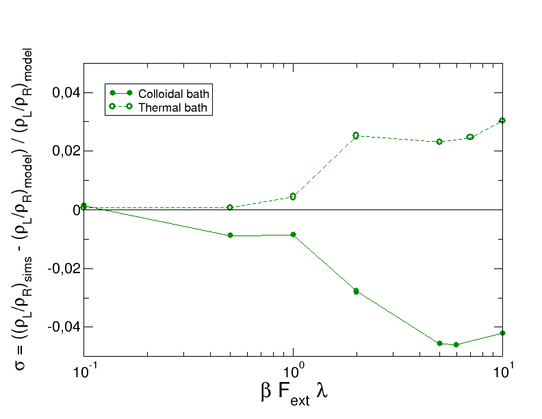
Figure 9: Relative difference, $\sigma$, between the theoretical prediction of $\rho_{L}/\rho_{R}$ and the numerical one, normalized by the theoretical value, for both colloidal and thermal bath (see legend) in the case $A/a=1$.

Longitudinal velocity of the tracer particle

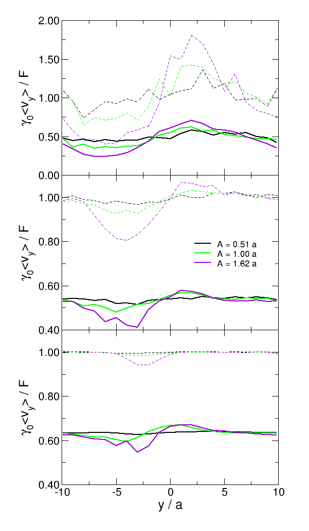
Figure 10: Component of the tracer velocity along the channel. The tracer velocity is averaged in slabs transverse to the channel direction as a function of the channel corrugation and applied external force for different corrugations and forces: $\beta F_{ext}\lambda=10$ (upper panel), $\beta F_{ext}\lambda=100$ (intermediate panel) and $\beta F_{ext}\lambda=1000$ (bottom panel). Solid lines stand for thermal bath whereas dashed lines for the colloidal bath.

Transverse velocity of the tracer particle

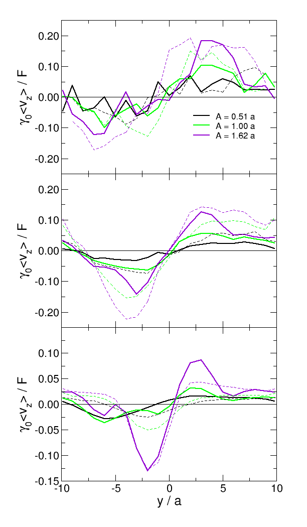
Figure 11: Component of the tracer velocity along the transverse direction. The tracer velocity is averaged in slabs transverse to the channel direction as a function of the channel corrugation and applied external force for different corrugations and forces: $\beta F_{ext}\lambda=10$ (upper panel), $\beta F_{ext}\lambda=100$ (intermediate panel) and $\beta F_{ext}\lambda=1000$ (bottom panel). Solid lines stand for the colloidal bath whereas dashed lines for the thermal bath.

First passage time distribution

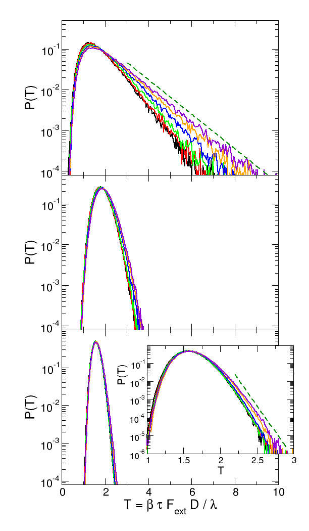
Figure 12: Distributions of first passage times for different corrugations (as indicated in the legend) and forces: $\beta F_{ext}\lambda=10$ (upper panel), $\beta F_{ext}\lambda=100$ (intermediate panel) and $\beta F_{ext}\lambda=1000$ (bottom panel). The inset to the bottom panel shows a zoom to the proper scale.

References

- Furst and Squires (2017) E. Furst and T. Squires, Microrheology (Oxford University Press, UK, 2017).
- Mason and Weitz (1995) T. G. Mason and D. A. Weitz, Phys. Rev. Lett. 74, 1250 (1995).
- Cicuta and Donald (2007) P. Cicuta and A. Donald, Soft Matter 3, 1449 (2007).
- Wilson and Poon (2011) L. G. Wilson and W. C. K. Poon, Phys. Chem. Chem. Phys. 13, 10617 (2011).
- Habdas et al. (2004) P. Habdas, D. Schaar, A. C. Levitt, and E. R. Weeks, Europhysics Letters (EPL) 67, 477 (2004).
- Squires and Brady (2005) T. Squires and J. F. Brady, Phys. Fluids 17, 073101 (2005).
- Gazuz et al. (2009) I. Gazuz, A. Puertas, T. Voigtmann, and M. Fuchs, Phys. Rev. Lett. 102, 248302 (2009).
- Puertas and Voigtmann (2014) A. Puertas and T. Voigtmann, J. Phys.: Condens. Matter 26, 243101 (2014).
- Zia (2018) R. N. Zia, Annual Review of Fluid Mechanics 50, 371 (2018).
- DePuit et al. (2011) R. DePuit, A. Khair, and T. Squires, Phys. Fluids 23, 063102 (2011).
- Chu and Zia (2019) H. C. Chu and R. N. Zia, Journal of Colloid and Interface Science 539, 388 (2019), ISSN 0021-9797.
- Gruber et al. (2016) M. Gruber, G. C. Abade, A. M. Puertas, and M. Fuchs, Phys. Rev. E 94, 042602 (2016).
- Su et al. (2017) Y. Su, J. W. Swan, and R. N. Zia, The Journal of Chemical Physics 146, 124903 (2017).
- Bénichou et al. (2014) O. Bénichou, P. Illien, G. Oshanin, A. Sarracino, and R. Voituriez, Phys. Rev. Lett. 113, 268002 (2014).
- Illien et al. (2014) P. Illien, O. Bénichou, G. Oshanin, and R. Voituriez, Phys. Rev. Lett. 113, 030603 (2014).
- Bénichou et al. (2016) O. Bénichou, P. Illien, G. Oshanin, A. Sarracino, and R. Voituriez, Phys. Rev. E 93, 032128 (2016).
- Bénichou et al. (2018) O. Bénichou, P. Illien, G. Oshanin, A. Sarracino, and R. Voituriez, Journal of Physics: Condensed Matter 30, 443001 (2018), URL https://doi.org/10.1088/1361-648x/aae13a.
- Gisler and Weitz (1999) T. Gisler and D. A. Weitz, Phys. Rev. Lett. 82, 1606 (1999).
- Oppong et al. (2006) F. K. Oppong, L. Rubatat, B. J. Frisken, A. E. Bailey, and J. R. de Bruyn, Phys. Rev. E 73, 041405 (2006).
- Prasad and Weeks (2009) V. Prasad and E. R. Weeks, Phys. Rev. Lett. 102, 178302 (2009).
- Weigand et al. (2017) W. Weigand, A. Messmore, J. Tu, A. Morales-Sanz, B. D.L., D. Beheyn, U. J.S., and R. Robertson-Anderson, PLoS One 12, e0176732 (2017).
- Nishizawa et al. (2017) K. Nishizawa, M. Bremerich, H. Ayade, C. F. Schmidt, T. Ariga, and D. Mizuno, Science Advances 3 (2017).
- Marconi et al. (2015) U. Marconi, P. Malgaretti, and I. Pagonabarraga, J. Chem. Phys. 134, 184501 (2015).
- Puertas et al. (2018) A. M. Puertas, P. Malgaretti, and I. Pagonabarraga, The Journal of Chemical Physics 149, 174908 (2018).
- Jacobs (1967) M. Jacobs, Diffusion Processes (Springer, New York, 1967).
- Zwanzig (1992) R. Zwanzig, J. Phys. Chem. 96, 3926 (1992).
- D. Reguera (2001) J. R. D. Reguera, Phys. Rev. E 64, 061106 (2001).
- Kalinay and Percus (2006) P. Kalinay and J. K. Percus, Phys. Rev. E 74, 049904 (2006).
- Pineda et al. (2012) I. Pineda, J. Alvarez-Ramirez, and L. Dagdug, J. Chem. Phys. 137, 174103 (2012).
- Berezhkovskii et al. (2015) A. M. Berezhkovskii, L. Dagdug, and S. M. Bezrukov, The Journal of Chemical Physics 143, 164102 (2015).
- Kalinay and Slanina (2018) P. Kalinay and F. Slanina, Journal of Physics: Condensed Matter 30, 244002 (2018).
- Malgaretti et al. (2013) P. Malgaretti, I. Pagonabarraga, and J. Rubi, Frontiers in Physics 1, 21 (2013).
- Martens et al. (2011) S. Martens, G. Schmid, L. Schimansky-Geier, and P. Hänggi, Phys. Rev. E 83, 051135 (2011).
- Martens et al. (2013) S. Martens, A. V. Straube, G. Schmid, L. Schimansky-Geier, and P. Hänggi, Phys. Rev. Lett. 110, 010601 (2013).
- Malgaretti et al. (2014) P. Malgaretti, I. Pagonabarraga, and J. M. Rubi, Phys. Rev. Lett 113, 128301 (2014).
- Chinappi and Malgaretti (2018) M. Chinappi and P. Malgaretti, Soft Matter 14, 9083 (2018).
- Malgaretti et al. (2019a) P. Malgaretti, M. Janssen, I. Pagonabarraga, and J. M. Rubi, J. Chem. Phys. 151, 084902 (2019a).
- Kalinay (2020) P. Kalinay, Phys. Rev. E 102, 042606 (2020).
- Bianco and Malgaretti (2016) V. Bianco and P. Malgaretti, J. Chem. Phys. 145, 114904 (2016).
- Malgaretti and Oshanin (2019) P. Malgaretti and G. Oshanin, Polymers 11 (2019).
- Carusela et al. (2021) M. F. Carusela, P. Malgaretti, and J. M. Rubi, Phys. Rev. E 103, 062102 (2021).
- Malgaretti and Harting (2021) P. Malgaretti and J. Harting, Soft Matter 17, 2062 (2021).
- Ledesma-Durán et al. (2016) A. Ledesma-Durán, S. I. Hernández-Hernández, and I. Santamaría-Holek, The Journal of Physical Chemistry C 120, 7810 (2016).
- Chacón-Acosta et al. (2020) G. Chacón-Acosta, M. Núñez López, and I. Pineda, The Journal of Chemical Physics 152, 024101 (2020).
- Malgaretti et al. (2016) P. Malgaretti, I. Pagonabarraga, and J. M. Rubi, J. Chem. Phys. 114, 034901 (2016).
- Carpen and Brady (2005) I. C. Carpen and J. F. Brady, Journal of Rheology 49, 1483 (2005).
- Metzler et al. (2014) R. Metzler, G. Oshanin, and S. Redner, First-Passage Phenomena and Their Applications (World Scientific Publishers, Singapore, 2014).
- Redner (2001) S. Redner, A guide to first passage processes (Cambridge University Press, Cambridge, 2001).
- Gardiner (1994) C. Gardiner, Handbook of stochastic methods : for physics, chemistry and the natural sciences (Springer, Berlin, 1994).
- Liétor-Santos et al. (2007) J. J. Liétor-Santos, M. Chávez-Páez, M. Márquez, A. Fernández-Nieves, and M. Medina-Noyola, Phys. Rev. E 76, 050403 (2007).
- Sandomirski et al. (2011) K. Sandomirski, E. Allahyarov, H. Löwen, and S. U. Egelhaaf, Soft Matter 7, 8050 (2011).
- Mansoori and Rice (2014) G. A. Mansoori and S. A. Rice, Confined Fluids: Structure, Properties and Phase Behavior (John Wiley and Sons, Ltd, 2014), chap. 5, p. 197, ISBN 9781118949702.
- Kjellander (2019) R. Kjellander, Statistical Mechanics of Liquids and Solutions: Intermolecular Forces, Structure and Surface Interactions (CRC Press, 2019), ISBN 9781482244045.
- Gravelle et al. (2011) A. Gravelle, Y. Peysson, R. Tabary, and P. Egermann, Transport in Porous Media 88, 441 (2011).
- Foroozesh and Kumar (2020) J. Foroozesh and S. Kumar, Journal of Molecular Liquids 316, 113876 (2020), ISSN 0167-7322.
- Zhang et al. (2020) B. Zhang, A. I. A. Mohamed, L. Goual, and M. Piri, Scientific Reports 10, 17539 (2020).
- Bizmark et al. (2020) N. Bizmark, J. Schneider, R. D. Priestley, and S. S. Datta, Science Advances 6 (2020).
- Bénichou et al. (2013) O. Bénichou, A. Bodrova, D. Chakraborty, P. Illien, A. Law, C. Mejía-Monasterio, G. Oshanin, and R. Voituriez, Phys. Rev. Lett. 111, 260601 (2013).
- Fourar et al. (2004) M. Fourar, G. Radilla, R. Lenormand, and C. Moyne, Advances in Water Resources 27, 669 (2004), ISSN 0309-1708.
- Malgaretti et al. (2019b) P. Malgaretti, G. Oshanin, and J. Talbot, Journal of Physics: Condensed Matter 31, 270201 (2019b).
- Muthukumar (2011) M. Muthukumar, Polymer translocation (CRC Press, Boca Raton, 2011).
- Ascher (1998) L. R. Ascher, Uri M. annd Petzold, Computer Methods for Ordinary Differential Equations and Differential-Algebraic Equations (Society for Industrial and Applied Mathematics, Philadelphia, 1998).