A model for lime consolidation of porous solids

Abstract

We propose a mathematical model describing the process of filling the pores of a building material with lime water solution with the goal to improve the consistency of the porous solid. Chemical reactions produce calcium carbonate which glues the solid particles together at some distance from the boundary and strengthens the whole structure. The model consists of a 3D convection-diffusion system with a nonlinear boundary condition for the liquid and for calcium hydroxide, coupled with the mass balance equations for the chemical reaction. The main result consists in proving that the system has a solution for each initial data from a physically relevant class. A 1D numerical test shows a qualitative agreement with experimental observations.

Keywords: porous media, reaction-diffusion, consolidation

2020 Mathematics Subject Classification: 35K51, 80A32, 92E20

Introduction

In this paper we investigate mathematically a process which is used by the building industry in order to protect and conserve cultural goods and other structure works. Such structures which are subject to weathering can be strengthened by filling the pores by a water-lime-mixture. The mixture penetrates into the pore structure of the stone and the calcium hydroxide reacts with carbon dioxide and builds calcium carbonate and water. A solid layer is built in the pore space which strengthens the material. The main problem is, however, that the consolidated layer is in practice rather thin and is located too close to the active boundary.

In order to avoid possible ambiguity, it is necessary to explain that the term ‘consolidation’ is to be interpreted here as a process of formation of calcium carbonate which has the property of binding the particles together. It might also be called ‘cementation’ or ‘compaction’.

In the literature there are a lot of works dealing with those problems. Different practical strategies for the wetting and drying regime which lead to a more uniform distribution of the consolidant are compared in [25]. A mathematical model is proposed in [31, 32], and [13], where the authors derive governing equations for moisture, heat, and air flow through concrete. A numerical procedure based on the finite element method is developed there to solve the set of equations and to investigate the influence of relative humidity and temperature. It is shown that the amount of calcium carbonate formed in a unit of time depends on the degree of carbonation, i. e., the availability of calcium hydroxide, the temperature, the carbon dioxide concentration and the relative humidity in the pore structure of the concrete. An extension of the aforementioned papers by studying the hygro-thermal behavior of concrete in the special situation of high temperatures can be found in [17].

In the present case chemical reactions take place. Various approaches exist which describe such processes by models which stem from different backgrounds (e. g., from mixture theory or empirical models). An overview on the development of theories especially for porous media including chemical reactions is given in [14]. The interactions between the constituents of a porous medium are not necessarily of chemical nature which would lead to a chemical transformation of one set of chemical substances to another. Simpler is the mass exchange between the constituents by physical processes like adsorption. Adsorption-diffusion processes have been studied by B. Albers (the former name of B. Detmann) e. g. in [2]. Other works on sorption in porous solids including molecular condensation are [5] or [6]. In these works the diffusivities of water and carbon dioxide are assumed to be strongly dependent on pore humidity, temperature and also on the degree of hydration of concrete. The authors realized that the porosity becomes non-uniform in time. This is an observation which is interesting also in the present case because the structure of the channels clearly changes with the progress of the reaction. A survey of consolidation techniques for historical materials is published in [27]. The influence of the particle size on the efficiency of the consolidation process is investigated in [35]. Experimental determination of the penetration depth is the subject of [7, 8, 9]. Different variants of the consolidants is studied in [15, 22, 28, 33], and an experimental work on mechanical interaction between the consolidant and the matrix material is carried out in [21].

A further work dealing with chemical reactions and diffusion in concrete based on the mixture theory for fluids introduced by Truesdell and coworkers is by A. J. Vromans et al. [37]. The model describes the corrosion of concrete with sulfuric acid which means a transformation of slaked lime and sulfuric acid into gypsum releasing water. It is a similar reaction we are looking at. A similar topic is dealt with in [36], where it is shown how the carbonation process in lime mortar is influenced by the diffusion of carbon dioxide into the mortar pore system by the kinetics of the lime carbonation reaction and by the drying and wetting process in the mortar.

Experimental results of $\mathrm{CaCO_{3}}$ precipitation kinetics can be found in [30]. The porosity changes during the reaction. This was studied by Houst and Wittmann, who also investigated the influence of the water content on the diffusivity of $\mathrm{CO_{2}}$ and $\mathrm{O_{2}}$ through hydrated cement paste [19]. An investigation of the physico-chemical characteristics of ancient mortars with comparison to a reaction-diffusion model by Zouridakis et al. is presented in [38]. A slightly different reaction involving also sulfur is mathematically studied in [10] by Böhm et al. There the corrosion in a sewer pipe is modeled as a moving-boundary system. A strategy for predicting the penetration of carbonation reaction fronts in concrete was proposed by Muntean et al. in [23]. A simple 1D mathematical model for the treatment of sandstone neglecting the effects of chemical reactions is proposed in [12] and further refined in [11].

We model the consolidation process as a convection-diffusion system coupled with chemical reaction in a 3D porous solid. The physical observation that only water can be evacuated from the porous body, while lime remains inside, requires a nonstandard boundary condition on the active part of the boundary. We choose a simple one-sided condition for the lime exchange between the interior and the exterior. The main result of the paper consists in proving rigorously that the resulting initial-boundary value problem for the PDE system in 3D has a solution satisfying natural physical constraints, including the boundedness of the concentrations proved by means of time discrete Moser iterations. We also show the result of numerical simulation in a simplified 1D situation.

The structure of the present paper is the following. In Section 1, we explain the modeling hypotheses and derive the corresponding system of balance equations with nonlinear boundary conditions. In Section 2, we give a rigorous formulation of the initial-boundary value problem, specify the mathematical hypotheses, and state the main result in Theorem 2.2. The solution is constructed by a time-discretization scheme proposed in Section 3. The estimates independent of the time step size derived for this time-discrete system constitute the substantial step in the proof of Theorem 2.2, which is obtained in Section 4 by passing to the limit as the time step tends to zero. A numerical test for a reduced 1D system is carried out in Section 5 to illustrate a qualitative agreement of the mathematical result with experimental observations.

1   The model

We imagine a porous medium (sandstone, for example) the structure of which is to be strengthened by letting calcium hydroxide particles driven by water flow penetrate into the pores. In contact with the air present in the pores, the calcium hydroxide reacts with the carbon dioxide contained in the air and produces a precipitate (calcium carbonate) which is not water-soluble, remains in the pores, and glues the sandstone particles together. Unlike, e. g., in [18, 34], we do not consider the porosity as one of the state variables. The porosity evolution law is replaced with the assumption that the permeability decreases as a result of the calcium carbonate deposit in the pores. The chemical reaction is assumed to be irreversible and we write it as $Ca(OH)_{2}+CO_{2}\to CaCO_{3}+H_{2}O$.

Notation:

• $\dot{c}^{W}$ … mass source rate of $H_{2}O$ produced by the chemical reaction

• $\dot{c}^{H}$ … mass source rate of $Ca(OH)_{2}$ produced by the chemical reaction

• $\dot{c}^{P}$ … mass source rate of $CaCO_{3}$ produced by the chemical reaction

• $\dot{c}^{G}$ … mass source rate of $CO_{2}$ produced by the chemical reaction

• $m^{W}$ … molar mass of $H_{2}O$

• $m^{H}$ … molar mass of $Ca(OH)_{2}$

• $m^{P}$ … molar mass of $CaCO_{3}$

• $m^{G}$ … molar mass of $CO_{2}$

• $\rho^{W}$ … mass density of $H_{2}O$

• $\rho^{H}$ … mass density of $Ca(OH)_{2}$

• $p$ … capillary pressure

• $s$ … water volume saturation

• ${h}$ … relative concentration of $Ca(OH)_{2}$

• $p^{\partial\Omega}$ … outer pressure

• $h^{\partial\Omega}$ … outer concentration of $Ca(OH)_{2}$

• $v$ … transport velocity vector

• $k(c^{P})$ … permeability of the porous solid

• $q$ … liquid mass flux

• $q^{H}$ … mass flux of $Ca(OH)_{2}$

• $\gamma$ … speed of the chemical reaction

• $\kappa$ … diffusivity of $Ca(OH)_{2}$

• $n$ … unit outward normal vector

• $\sigma(x)$ … transport velocity interaction kernel

• $\alpha(x)$ … boundary permeability for water

• $\beta(x)$ … boundary permeability for the inflow of $Ca(OH)_{2}$

Mass balance of the chemical reaction:

$$\frac{\dot{c}^{P}}{m^{P}}=\frac{\dot{c}^{W}}{m^{W}}=-\frac{\dot{c}^{H}}{m^{H}}=-\frac{\dot{c}^{G}}{m^{G}}.$$

Water mass balance in an arbitrary subdomain $V$ of the porous body:

$$\frac{\,\mathrm{d}}{\,\mathrm{d}t}\int_{V}\rho^{W}s\,\mathrm{d}x+\int_{\partial V}q\cdot n\,\mathrm{d}S=\int_{V}\dot{c}^{W}\,\mathrm{d}x.$$

Calcium hydroxide mass balance in an arbitrary subdomain $V$ of the porous body:

$$\frac{\,\mathrm{d}}{\,\mathrm{d}t}\int_{V}\rho^{H}{h}\,\mathrm{d}x+\int_{\partial V}q^{H}\cdot n\,\mathrm{d}S=\int_{V}\dot{c}^{H}\,\mathrm{d}x.$$

Water mass balance in differential form:

$$\rho^{W}\dot{s}+\mathrm{\,div\,}q=\dot{c}^{W}.$$

Calcium hydroxide mass balance in differential form:

$$\rho^{H}\dot{h}+\mathrm{\,div\,}q^{H}=\dot{c}^{H}.$$

The water mass flux is assumed to obey the Darcy law:

$$q=-k(c^{P})\nabla p,$$

with permeability coefficient $k(c^{P})$ which is assumed to decrease as the amount $c^{P}$ of $CaCO_{3}$ given by the formula

$$c^{P}(x,t)=\int_{0}^{t}\dot{c}^{P}(x,t^{\prime})\,\mathrm{d}t^{\prime}$$

increases and fills the pores.

The flux of $Ca(OH)_{2}$ consists of transport and diffusion terms:

$$q^{H}=\rho^{H}{h}v-\kappa s\nabla{h}.$$

The mobility coefficient $\kappa s$ in the diffusion term is assumed to be proportional to $s$: If there is no water in the pores, no diffusion takes place.

We assume that the transport of $Ca(OH)_{2}$ at the point $x\in\Omega$ is driven by the water flux in a small neighborhood of $x$. In mathematical terms, we assume that there exists a nonnegative function $\sigma$ with support in a small neighborhood of the origin such that the transport velocity $v$ can be defined as

$$v(x,t)=\frac{1}{\rho^{H}}\int_{\Omega}\sigma(x-y)q(y,t)\,\mathrm{d}y.$$

The main reason for this assumption is a mathematical one. The strong nonlinear coupling between $s$ and $h$ makes it difficult to control the bounds for the unknowns in the approximation scheme. We believe that such a regularization of the transport velocity makes physically sense as well.

The wetting-dewetting curve is described by an increasing function $f$:

$$p=f(s).$$

We focus on modeling the chemical reactions. Capillary hysteresis, deformations of the solid matrix, and thermal effects are therefore neglected here. We plan to include them following the ideas of [3] in a subsequent study.

The dynamics of the chemical reaction is modeled according to the so-called law of mass action, which states that the rate of the chemical reaction is directly proportional to the product of the concentrations of the reactants. We assume it in the form

$$\dot{c}^{P}=\gamma m^{P}{h}s(1-s).$$ (1.1)

Its meaning is that no reaction can take place if either no $Ca(OH)_{2}$ is available (that is, $h=0$), or no water is available (that is, $s=0$), or no $CO_{2}$ is available (that is, $s=1$), according to the hypothesis that the chemical reaction takes dominantly place on the contact between water and air. In order to reduce the complexity of the problem, we assume directly that the available quantity of $CO_{2}$ is proportional to the air content.

On the boundary $\partial\Omega$ we prescribe the normal fluxes. For the normal component of $q$, we assume that it is proportional to the difference between the pressures $p$ inside and $p^{\partial\Omega}$ outside the body. For the flux of $Ca(OH)_{2}$, we assume that it can point only inward proportionally to the difference of concentrations and to $s$, and no outward flux is possible. Inward flux takes place only if the outer concentration $h^{\partial\Omega}$ is bigger than the inner concentration $h$:

$$\left.\begin{array}[]{rcl}q\cdot n&=&\alpha(x)(p-p^{\partial\Omega})\\[4.2679pt] q^{H}\cdot n&=&-\beta(x)s(h^{\partial\Omega}-h)^{+}\end{array}\right\}\text{on }\partial\Omega.$$

2   Mathematical problem

Let $\Omega\subset\mathbb{R}^{3}$ be a bounded Lipschitzian domain. We consider the Hilbert triplet $V\subset H\equiv H^{\prime}\subset V^{\prime}$ with compact embeddings and with $H=L^{2}(\Omega)$, $V=W^{1,2}(\Omega)$. For two unknown functions $s(x,t),h(x,t)$ defined for $(x,t)\in\Omega\times(0,T)$ the resulting PDE system reads

$$\int_{\Omega}(\rho^{W}s_{t}\phi(x)+k(c^{P})f^{\prime}(s)\nabla s\cdot\nabla\phi(x))\,\mathrm{d}x+\int_{\partial\Omega}\alpha(x)(f(s)-f(s^{\partial\Omega}))\phi(x)\,\mathrm{d}S(x)$$

$$\qquad=\gamma m^{W}\int_{\Omega}{h}s(1-s)\phi(x)\,\mathrm{d}x,$$ (2.1)

$$\int_{\Omega}(\rho^{H}h_{t}\psi(x)+(\kappa s\nabla{h}-\rho^{H}hv)\cdot\nabla\psi(x))\,\mathrm{d}x-\int_{\partial\Omega}\beta(x)s(h^{\partial\Omega}-h)^{+}\psi(x)\,\mathrm{d}S(x)$$

$$\qquad=-\gamma m^{H}\int_{\Omega}{h}s(1-s)\psi(x)\,\mathrm{d}x.$$ (2.2)

for all test functions $\phi,\psi\in V$, where $s^{\partial\Omega}:=f^{-1}(p^{\partial\Omega})$, and with initial conditions

$$s(x,0)=s^{0}(x),\quad h(x,0)=h^{0}(x)\quad\mathrm{for\ }x\in\Omega.$$ (2.3)

Hypothesis 2.1.

The data have the properties

• $s^{\partial\Omega}\in L^{\infty}(\partial\Omega\times(0,T))$, $s^{0}\in L^{\infty}(\Omega)\cap W^{1,2}(\Omega)$ are given such that $s^{\partial\Omega}_{t}\in L^{2}(\partial\Omega\times(0,T))$, $0<s^{\flat}\leq s^{\partial\Omega}(x,t)\leq 1$ for a. e. $(x,t)\in\partial\Omega{\times}(0,T)$, $0<s^{\flat}\leq s^{0}(x)\leq 1$ for a. e. $x\in\Omega$;

• $h^{\partial\Omega}\in L^{\infty}(\partial\Omega\times(0,T))$, $h^{0}\in L^{\infty}(\Omega)$ are given such that $0\leq h^{\partial\Omega}(x,t)\leq h^{\sharp}$ for a. e. $(x,t)\in\partial\Omega\times(0,T)$, $0\leq h^{0}(x)\leq h^{\sharp}$ for some $h^{\sharp}>0$ and for a. e. $x\in\Omega$;

• $f:[0,1]\to\mathbb{R}$ is continuously differentiable, $0<f^{\flat}\leq f^{\prime}(s)\leq f^{\sharp}$ for $0\leq s\leq 1$;

• $k$ is continuously differentiable and nonincreasing, $0<k^{\flat}\leq k(r)\leq k^{\sharp}$ for $r\geq 0$;

• $\sigma:\mathbb{R}^{3}\to[0,\infty)$ is continuous with compact support, $\int_{\mathbb{R}^{3}}\sigma(x)\,\mathrm{d}x=1$;

• $\alpha,\beta\in L^{\infty}(\partial\Omega)$, $\alpha(x)\geq 0$, $\beta(x)\geq 0$ on $\partial\Omega$, $\int_{\partial\Omega}\alpha(x)\,\mathrm{d}S(x)>0$, $\int_{\partial\Omega}\beta(x)\,\mathrm{d}S(x)>0$.

The meaning of Hypothesis 2.1 (vi) is that the boundary $\partial\Omega$ is inhomogeneous, with different permeabilities at different parts of the boundary. The transport of water (supply of $Ca(OH)_{2}$) through the boundary takes place only on parts of $\partial\Omega$ where $\alpha>0$ ($\beta>0$, respectively).

The remaining sections are devoted to the proof of the following result.

Theorem 2.2.

Let Hypothesis 2.1 hold. Then system (2.1)–(2.2) with initial conditions (2.3) admits a solution $(s,h)$ such that $s_{t}\in L^{2}(\Omega\times(0,T))$, $\nabla s\in L^{\infty}(0,T;L^{2}(\Omega;\mathbb{R}^{3}))$, $\nabla h\in L^{2}(\Omega\times(0,T);\mathbb{R}^{3})$, $h_{t}\in L^{2}(0,T;W^{-1,2}(\Omega))$, $h\in L^{\infty}(\Omega\times(0,T))$, $s(x,t)\in[0,1]$ a. e., $h(x,t)\geq 0$ a. e.

We omit the positive physical constants which are not relevant for the analysis. The strategy of the proof is based on choosing a cut-off parameter $R>0$, replacing $h$ in the nonlinear terms with $Q_{R}(h)=\min\{h^{+},R\}$, $1-s$ with $Q_{R}(1-s)$, and $v$ in (2.2) with $v^{R}:=(Q_{R}(|v|)/|v|)v$. We also extend the values of the function $f$ outside the interval $[0,1]$ by introducing the function $\tilde{f}$ by the formula

$$\tilde{f}(s)=\left\{\begin{array}[]{ll}f(0)+f^{\prime}(0)s&\mathrm{for\ }s<0,\\ f(s)&\mathrm{for\ }s\in[0,1],\\ f(1)+f^{\prime}(1)(s-1)&\mathrm{for\ }s>1,\end{array}\right.$$

and consider the system

$$\int_{\Omega}(s_{t}\phi(x)+k(c^{P})\tilde{f}^{\prime}(s)\nabla s\cdot\nabla\phi(x))\,\mathrm{d}x+\int_{\partial\Omega}\alpha(x)(\tilde{f}(s)-\tilde{f}(s^{\partial\Omega}))\phi(x)\,\mathrm{d}S(x)$$

$$\qquad=\int_{\Omega}Q_{R}(h)sQ_{R}(1-s)\phi(x)\,\mathrm{d}x,$$ (2.4)

$$\int_{\Omega}(h_{t}\psi(x)+(s\nabla{h}-hv^{R})\cdot\nabla\psi(x))\,\mathrm{d}x-\int_{\partial\Omega}\beta(x)s(h^{\partial\Omega}-h)^{+}\psi(x)\,\mathrm{d}S(x)$$

$$\qquad=-\int_{\Omega}{h}s(1-s)\psi(x)\,\mathrm{d}x$$ (2.5)

for all $\phi,\psi\in V$. We first construct and solve in Section 3 a time-discrete approximating system of (2.4)–(2.5), and derive estimates independent of the time step. In Section 4, we let the time step tend to $0$ and prove that the limit is a solution $(s,h)$ to (2.4)–(2.5). We also prove that this solution has the property that $s\in[0,1]$, $h$ is positive and bounded, and $v$ is bounded, so that for $R$ sufficiently large, the truncations are never active and the solution thus satisfies (2.1)–(2.2) as well.

3   Time discretization

For proving Theorem 2.2, we first choose $n\in\mathbb{N}$ and replace (2.4)–(2.5) with the following time-discrete system with time step $\tau=\frac{T}{n}$:

$$\int_{\Omega}\left(\frac{1}{\tau}(s_{j}-s_{j-1})\phi(x)+k(c^{P}_{j-1})\tilde{f}^{\prime}(s_{j})\nabla s_{j}\cdot\nabla\phi(x)\right)\,\mathrm{d}x+\int_{\partial\Omega}\alpha(x)(\tilde{f}(s_{j})-\tilde{f}(s^{\partial\Omega}_{j}))\phi(x)\,\mathrm{d}S(x)$$

$$\qquad=\int_{\Omega}Q_{R}(h_{j-1})s_{j}Q_{R}(1-s_{j})\phi(x)\,\mathrm{d}x,$$ (3.1)

$$\int_{\Omega}\left(\frac{1}{\tau}(h_{j}{-}h_{j-1})\psi(x)+(s_{j-1}\nabla{h_{j}}{-}h_{j}v^{R}_{j-1})\cdot\nabla\psi(x)\right)\,\mathrm{d}x-\int_{\partial\Omega}\beta(x)s_{j-1}(h^{\partial\Omega}_{j}-h_{j})^{+}\psi(x)\,\mathrm{d}S(x)$$

$$\qquad=-\int_{\Omega}{h_{j}}s_{j-1}(1-s_{j-1})\psi(x)\,\mathrm{d}x,$$ (3.2)

for $j=1,\dots,n$ with initial conditions $s_{0}=s^{0}$, $h_{0}=h^{0}$, and with $c^{P}_{i}=0$ for $i\leq 0$, with

$$q_{j}(x) =-k(c^{P}_{j}(x))\nabla\tilde{f}(s_{j}(x)) \mathrm{for\ }\ x\in\Omega,$$ (3.3)

$$v_{j}(x) =\int_{\Omega}\sigma(x-y)q_{j}(y)\,\mathrm{d}y \mathrm{for\ }\ x\in\Omega,$$ (3.4)

$$s^{\partial\Omega}_{j}(x) =\frac{1}{\tau}\int_{t_{j-1}}^{t_{j}}s^{\partial\Omega}(x,t)\,\mathrm{d}t \mathrm{for\ }\ x\in\partial\Omega,$$ (3.5)

$$h^{\partial\Omega}_{j}(x) =\frac{1}{\tau}\int_{t_{j-1}}^{t_{j}}h^{\partial\Omega}(x,t)\,\mathrm{d}t \mathrm{for\ }\ x\in\partial\Omega,$$ (3.6)

where $t_{j}=j\tau$ for $j=0,1,\dots,n$. Moreover, we define inductively

$$c^{P}_{j}-c^{P}_{j-1}=\tau h_{j}s_{j}(1-s_{j})\ \mbox{ for }\ j=1,\dots,n.$$ (3.7)

We now prove the existence of solutions to (3.1)–(3.2) and derive a series of estimates which will allow us to pass to the limit as $n\to\infty$. We denote by $C$ any positive constant depending possibly on the data and independent of $n$.

For $\varepsilon>0$ we denote by $H_{\varepsilon}:\mathbb{R}\to\mathbb{R}$ the function

$$H_{\varepsilon}(r)=\left\{\begin{array}[]{ll}0&\mathrm{for\ }r\leq 0,\\[5.69054pt] \frac{r}{\varepsilon}&\mathrm{for\ }r\in(0,\varepsilon),\\[5.69054pt] 1&\mathrm{for\ }r\geq\varepsilon\end{array}\right.$$ (3.8)

as a Lipschitz continuous regularization of the Heaviside function, and by $\hat{H}_{\varepsilon}$ its antiderivative

$$\hat{H}_{\varepsilon}(r)=\left\{\begin{array}[]{ll}0&\mathrm{for\ }r\leq 0,\\[5.69054pt] \frac{r^{2}}{2\varepsilon}&\mathrm{for\ }r\in(0,\varepsilon),\\[5.69054pt] r-\frac{\varepsilon}{2}&\mathrm{for\ }r\geq\varepsilon\end{array}\right.$$ (3.9)

as a continuously differentiable approximation of the “positive part” function. Note that we have $rH_{\varepsilon}(r)\leq 2\hat{H}_{\varepsilon}(r)$ for all $r\in\mathbb{R}$.

Lemma 3.1.

Let Hypothesis 2.1 hold. Then for all $n$ sufficiently large there exists a solution $h_{j},\,s_{j}$ of the time-discrete system (3.1)–(3.2) with initial conditions $s_{0}=s^{0}$, $h_{0}=h^{0}$, $c^{P}_{i}=0$ for $i\leq 0$, which satisfies the bounds:

$$s^{\flat}\leq s_{j}(x)\leq 1\quad a.\,e.\quad\mathrm{for\ }j=0,1,\dots,n.$$ (3.10)

$$h_{j}(x)\geq 0\quad a.\,e.\quad\mathrm{for\ }j=0,1,\dots,n.$$ (3.11)

Proof.

To prove the existence, we proceed by induction. Assume that the solution to (3.1)-(3.2) is available for $i=1,\dots,j-1$ with the properties (3.10)–(3.11). Then Eq. (3.1) for the unknown $s:=s_{j}$ is of the form

$$\int_{\Omega}(a_{0}(x,s)\phi(x)+a_{1}(x)\tilde{f}^{\prime}(s)\nabla s\cdot\nabla\phi(x))\,\mathrm{d}x+\int_{\partial\Omega}\alpha(x)(\tilde{f}(s)-a_{2}(x))\phi(x)\,\mathrm{d}S(x)$$ (3.12)

$$=\int_{\Omega}a_{3}(x)\phi(x)\,\mathrm{d}x,$$

where

$$a_{0}(x,s)=\frac{1}{\tau}s(x)-Q_{R}(h_{j-1}(x))s(x)Q_{R}(1-s(x))$$

and $a_{k}$, $k=1,2,3$, are given functions which are known from the previous step $j-1$. For $n>TR^{2}$ the function $s\mapsto a_{0}(x,s)$ is increasing. Hence, (3.12) is a monotone elliptic problem, and a unique solution exists by virtue of the Browder-Minty Theorem, see [29, Theorem 10.49]. Similarly, Eq. (3.2) is for the unknown function $h:=h_{j}$ of the form

$$\int_{\Omega}(a_{4}(x)h\psi(x)+(a_{5}(x)\nabla h-a_{6}(x)h)\cdot\nabla\psi(x))\,\mathrm{d}x-\int_{\partial\Omega}\beta(x)a_{7}(x)(a_{8}(x)-h)^{+}\psi(x)\,\mathrm{d}S(x)$$

$$\qquad=\int_{\Omega}a_{9}(x)\psi(x)\,\mathrm{d}x,$$ (3.13)

which we can solve in an elementary way in two steps. First, we consider the PDE

$$\int_{\Omega}(a_{4}(x)h\psi(x)+(a_{5}(x)\nabla h-a_{6}(x)w)\cdot\nabla\psi(x))\,\mathrm{d}x-\int_{\partial\Omega}\beta(x)a_{7}(x)(a_{8}(x)-h)^{+}\psi(x)\,\mathrm{d}S(x)$$

$$\qquad=\int_{\Omega}a_{9}(x)\psi(x)\,\mathrm{d}x$$ (3.14)

with a given function $w\in L^{2}(\Omega)$. Here again the functions $a_{k}$, $k=4,\dots,9$, are known. We find a solution $h$ to (3.14) once more by the Browder-Minty Theorem. Since $a_{4}(x)\geq\frac{1}{\tau}$, $a_{5}(x)=s_{j-1}(x)\geq s^{\flat}$, and $a_{6}(x)=v_{j-1}^{R}\in[-R,R]$, we see that for $n>TR^{2}/2s^{\flat}$, the mapping which with $w$ associates $h$ is a contraction on $L^{2}(\Omega)$, and the solution to (3.13) is obtained from the Banach Contraction Principle.

To derive the bounds for the solution, we first test (3.1) by $\phi=H_{\varepsilon}(s_{j}-1)$ (or any other function of the form $g(s_{j}-1)$ with $g$ Lipschitz continuous, nondecreasing, and such that $g(s)=0$ for $s\leq 0$). The right-hand side identically vanishes, whereas the boundary term and $\nabla s_{j}\cdot\nabla H_{\varepsilon}(s_{j}-1)$ are nonnegative, which yields that

$$\int_{\Omega}(s_{j}-s_{j-1})H_{\varepsilon}(s_{j}-1)\,\mathrm{d}x\leq 0.$$

From the convexity of $\hat{H}_{\varepsilon}$ we obtain that $(s_{j}-s_{j-1})H_{\varepsilon}(s_{j}-1)\geq\hat{H}_{\varepsilon}(s_{j}-1)-\hat{H}_{\varepsilon}(s_{j-1}-1)$, hence,

$$\int_{\Omega}\hat{H}_{\varepsilon}(s_{j}-1)\,\mathrm{d}x\leq\int_{\Omega}\hat{H}_{\varepsilon}(s_{j-1}-1)\,\mathrm{d}x.$$

We have by hypothesis $s_{j-1}\leq 1$ a. e., and by induction we get

$$s_{j}(x)\leq 1\quad a.\,e.\quad\mathrm{for\ }j=0,1,\dots,n.$$ (3.15)

We further test (3.1) by $\phi=-H_{\varepsilon}(s^{\flat}-s_{j})$. Then both the boundary term and the elliptic term give a nonnegative contribution, and using again the convexity of $\hat{H}_{\varepsilon}$ we have

$$\frac{1}{\tau}\int_{\Omega}(\hat{H}_{\varepsilon}(s^{\flat}-s_{j})-\hat{H}_{\varepsilon}(s^{\flat}-s_{j-1}))\,\mathrm{d}x \leq\int_{\Omega}-s_{j}H_{\varepsilon}(s^{\flat}-s_{j})Q_{R}(h_{j-1})Q_{R}(1-s_{j})\,\mathrm{d}x$$

$$\leq\int_{\Omega}(s^{\flat}-s_{j})H_{\varepsilon}(s^{\flat}-s_{j})Q_{R}(h_{j-1})Q_{R}(1-s_{j})\,\mathrm{d}x$$

$$\leq 2R^{2}\int_{\Omega}\hat{H}_{\varepsilon}(s^{\flat}-s_{j})\,\mathrm{d}x,$$

and from the induction hypothesis we get for $n>2TR^{2}$ that

$$s_{j}(x)\geq s^{\flat}\quad a.\,e.\quad\mathrm{for\ }j=0,1,\dots,n.$$ (3.16)

We have in particular $Q_{R}(1-s_{j})=1-s_{j}$ for $R\geq 1$ as well as $\tilde{f}=f$.

Test (3.2) by $\psi=-H_{\varepsilon}(-h_{j})$. Then

$$\frac{1}{\tau}\int_{\Omega}(\hat{H}_{\varepsilon}(-h_{j})-\hat{H}_{\varepsilon}(-h_{j-1}))\,\mathrm{d}x+\int_{\Omega}s^{\flat}H^{\prime}_{\varepsilon}(-h_{j})|\nabla h_{j}|^{2}\,\mathrm{d}x\leq\int_{\Omega}h_{j}H^{\prime}_{\varepsilon}(-h_{j})v^{R}_{j-1}\cdot\nabla h_{j}\,\mathrm{d}x$$

$$\qquad\leq\frac{s^{\flat}}{2}\int_{\Omega}H^{\prime}_{\varepsilon}(-h_{j})|\nabla h_{j}|^{2}\,\mathrm{d}x+\frac{1}{2s^{\flat}}\int_{\Omega}h_{j}^{2}|v^{R}_{j-1}|^{2}H^{\prime}_{\varepsilon}(-h_{j})\,\mathrm{d}x$$

We have $0\leq h_{j}^{2}H^{\prime}_{\varepsilon}(-h_{j})\leq\varepsilon$ and $\lim_{\varepsilon\to 0}\hat{H}_{\varepsilon}(-h_{j})=(-h_{j})^{+}$, hence, passing to the limit as $\varepsilon\to 0$, by induction we get (3.11). ∎

Lemma 3.2.

Let Hypothesis 2.1 hold. Then $h_{j}$ satisfies the following estimate

$$\int_{\Omega}h_{j}(x)\,\mathrm{d}x\leq C$$ (3.17)

independently of $j=0,1,\dots,n$.

Proof.

Test (3.2) by $\psi=1$. Note that the boundary term is bounded above by a multiple of $h^{\sharp}$ and the right-hand side is negative or zero, so that

$$\frac{1}{\tau}\int_{\Omega}(h_{j}-h_{j-1})\,\mathrm{d}x\leq\hat{C},$$

that is,

$$\int_{\Omega}h_{j}\,\mathrm{d}x\leq\tau\hat{C}+\int_{\Omega}h_{j-1}\,\mathrm{d}x.$$

Summing up over $j=1,\dots,j^{*}$ we get

$$\int_{\Omega}h_{j^{*}}(x)\,\mathrm{d}x\leq\int_{\Omega}h_{0}(x)\,\mathrm{d}x+T\hat{C},$$

for an arbitrary $j^{*}$, which yields (3.17). ∎

The main issue will be a uniform upper bound for $h_{j}$ which will be obtained by a time-discrete variant of the Moser-Alikakos iteration technique presented in [4]. We start from some preliminary integral estimates of $s_{j}$.

Lemma 3.3.

Let Hypothesis 2.1 hold. Then $s_{j}$ satisfy the bounds

$$\tau\sum_{j=1}^{n}\int_{\Omega}|\nabla s_{j}(x)|^{2}\,\mathrm{d}x+\tau\sum_{j=1}^{n}\int_{\partial\Omega}\alpha(x)s_{j}^{2}(x)\,dS(x)\leq C,$$ (3.18)

$$\frac{1}{\tau}\sum_{j=1}^{n}\int_{\Omega}|s_{j}-s_{j-1}|^{2}\,\mathrm{d}x+\max_{j=1,\dots,n}\int_{\Omega}|\nabla s_{j}(x)|^{2}\,\mathrm{d}x\leq C\left(1+\tau\sum_{j=0}^{n}\int_{\Omega}h^{2}_{j}(x)\,\mathrm{d}x\right).$$ (3.19)

Proof.

Test (3.1) by $\phi=s_{j}$. From (3.17) we then obtain:

$$\frac{1}{2\tau}\int_{\Omega}(s_{j}^{2}-s_{j-1}^{2})\,\mathrm{d}x+\frac{f^{\flat}}{2}\int_{\partial\Omega}\alpha(x)s_{j}^{2}(x)\,dS(x)+k^{\flat}f^{\flat}\,\int_{\Omega}|\nabla s_{j}(x)|^{2}\,\mathrm{d}x$$

$$\leq C\int_{\partial\Omega}\alpha(x)\,dS(x)+\int_{\Omega}h_{j-1}\,\mathrm{d}x\leq C.$$

Taking the sum with respect to $j=1,\dots,n$ yields

$$\tau\sum_{j=1}^{n}\int_{\Omega}|\nabla s_{j}(x)|^{2}\,\mathrm{d}x+\tau\sum_{j=1}^{n}\int_{\partial\Omega}\alpha(x)s_{j}^{2}(x)\,dS(x)\leq C+\int_{\Omega}s_{0}^{2}\,\mathrm{d}x\leq C,$$

which is precisely (3.18).

Let us prove (3.19) now. Test (3.1) by $\phi=f(s_{j})-f(s_{j-1})$. Then

$$\frac{f^{\flat}}{\tau}\int_{\Omega}|s_{j}-s_{j-1}|^{2}\,\mathrm{d}x+\frac{1}{2}\int_{\Omega}\left(k(c^{P}_{j-1})|\nabla f(s_{j})|^{2}-k(c^{P}_{j-2})|\nabla f(s_{j-1})|^{2}\right)\,\mathrm{d}x$$

$$\qquad\qquad+\frac{1}{2}\int_{\partial\Omega}\alpha(x)(f^{2}(s_{j})-f^{2}(s_{j-1}))\,\mathrm{d}S(x)$$

$$\qquad\leq\frac{1}{2}\int_{\Omega}(k(c^{P}_{j-1})-k(c^{P}_{j-2}))|\nabla f(s_{j-1})|^{2}\,\mathrm{d}x+\int_{\partial\Omega}\alpha(x)(f(s_{j})f(s_{j}^{\partial\Omega})-f(s_{j-1})f(s_{j-1}^{\partial\Omega}))\,\mathrm{d}S(x)$$

$$\qquad\qquad+\left(\int_{\partial\Omega}\alpha(x)f^{2}(s_{j-1})\,\mathrm{d}S(x)\right)^{1/2}\,\left(\int_{\partial\Omega}\alpha(x)|f(s_{j-1}^{\partial\Omega})-f(s_{j}^{\partial\Omega})|^{2}\,\mathrm{d}S(x)\right)^{1/2}$$

$$\qquad\qquad+\int_{\Omega}h_{j-1}(f(s_{j})-f(s_{j-1}))\,\mathrm{d}x.$$ (3.20)

The function $k$ is nonincreasing and the sequence $\{c^{P}_{j}\}$ is nondecreasing, so the first integral in the right-hand side of (3.20) is negative. By Hypotheses 2.1 (i),(iii) and (3.5) we further have

$$\frac{1}{\tau}\sum_{j=1}^{n}\int_{\partial\Omega}\alpha(x)|f(s_{j}^{\partial\Omega})-f(s_{j-1}^{\partial\Omega})|^{2}\,\mathrm{d}S(x)\leq C,$$

and from (3.18) it follows that

$$\tau\sum_{j=1}^{n}\int_{\partial\Omega}\alpha(x)f^{2}(s_{j-1})\,\mathrm{d}S(x)\leq C,$$

hence, by Hölder’s inequality for sums,

$$\sum_{j=1}^{n}\left(\int_{\partial\Omega}\alpha(x)f^{2}(s_{j-1})\,\mathrm{d}S(x)\right)^{1/2}\,\left(\int_{\partial\Omega}\alpha(x)|f(s_{j-1}^{\partial\Omega})-f(s_{j}^{\partial\Omega})|^{2}\,\mathrm{d}S(x)\right)^{1/2}\leq C.$$

Applying Young’s inequality to the last integral in the right hand side we similarly have

$$\int_{\Omega}h_{j-1}(f(s_{j})-f(s_{j-1}))\,\mathrm{d}x\leq C\tau\int_{\Omega}h^{2}_{j-1}\,\mathrm{d}x+\frac{f^{\flat}}{2\tau}\int_{\Omega}|s_{j}-s_{j-1}|^{2}\,\mathrm{d}x.$$

Hence, taking the sum with respect to $j$ and using again (3.18), we get (3.19). ∎

Remark 3.4.

As a consequence of the definition of $v_{j}$ and $v^{R}_{j}$, we get for all $j=1,\dots,n$ that

$$\mathop{\rm sup\,ess\,}_{x\in\Omega}|v^{R}_{j}(x)|\leq\mathop{\rm sup\,ess\,}_{x\in\Omega}|v_{j}(x)|\leq C\left(1+\left(\int_{\Omega}|\nabla s_{j}(x)|^{2}\,\mathrm{d}x\right)^{1/2}\right).$$ (3.21)

Lemma 3.5.

Let Hypothesis 2.1 hold. Then $h_{j}$ satisfies the bound

$$\max_{j=1,\dots,n}\int_{\Omega}|h_{j}(x)|^{2}\,\mathrm{d}x+\tau\sum_{j=1}^{n}\int_{\Omega}|\nabla h_{j}(x)|^{2}\,\mathrm{d}x\leq C.$$ (3.22)

Proof.

Test (3.2) by $\psi=h_{j}$. Note that the boundary term is bounded above by a multiple of $(h^{\sharp})^{2}$. Then

$$\frac{1}{2\tau}\int_{\Omega}(h_{j}^{2}-h_{j-1}^{2})\,\mathrm{d}x+s^{\flat}\int_{\Omega}|\nabla h_{j}(x)|^{2}\,\mathrm{d}x\leq C+K_{j}$$ (3.23)

with $K_{j}:=\int_{\Omega}h_{j}v^{R}_{j-1}\cdot\nabla h_{j}\,\mathrm{d}x$. The evaluation of this integral constitutes the most delicate part of the argument. For simplicity, we denote by $|\cdot|_{r}$ the norm in $L^{r}(\Omega)$ for $1\leq r\leq\infty$. We first notice that by Hölder’s inequality and (3.21) we have

$$K_{j}\leq C(1+|h_{j}|_{2}|\nabla s_{j-1}|_{2}|\nabla h_{j}|_{2}).$$

Let us recall the Gagliardo-Nirenberg inequality for functions $u\in W^{1,p}(\Omega)$ on bounded Lipschitzian domains $\Omega\subset\mathbb{R}^{N}$ in the form

$$|u|_{q}\leq C\left(|u|_{s}+|u|_{s}^{1-\nu}|\nabla u|_{p}^{\nu}\right)$$ (3.24)

which goes back to [16, 26] and holds for every $s\leq p\leq q$ such that $\frac{1}{q}\geq\frac{1}{p}-\frac{1}{N}$, where

$$\nu=\frac{\frac{1}{s}-\frac{1}{q}}{\frac{1}{N}+\frac{1}{s}-\frac{1}{p}}.$$ (3.25)

In our case we have

$$|h_{j}|_{2}\leq C\left(|h_{j}|_{1}+|h_{j}|_{1}^{1-\nu}|\nabla h_{j}|_{2}^{\nu}\right)$$ (3.26)

with $\nu=3/5$. Hence, by (3.11) and (3.17),

$$K_{j}\leq C\left(1+|\nabla s_{j-1}|_{2}|\nabla h_{j}|_{2}^{8/5}\right).$$

Using Hölder’s inequality once again we obtain

$$\tau\sum_{j=1}^{n}K_{j}\leq C\left(1+\left(\tau\sum_{j=1}^{n}|\nabla s_{j-1}|_{2}^{5}\right)^{1/5}\left(\tau\sum_{j=1}^{n}|\nabla h_{j}|_{2}^{2}\right)^{4/5}\right).$$

We have

$$\tau\sum_{j=1}^{n}|\nabla s_{j-1}|_{2}^{5}\leq\tau\max_{j=0,\dots,n}|\nabla s_{j}|_{2}^{3}\sum_{j=0}^{n}|\nabla s_{j}|_{2}^{2},$$

and (3.18)–(3.19) together with (3.26) yield

$$\tau\sum_{j=1}^{n}|\nabla s_{j-1}|_{2}^{5}\leq C\left(1+\left(\tau\sum_{j=1}^{n}|h_{j}|_{2}^{2}\right)^{3/2}\right)\leq C\left(1+\left(\tau\sum_{j=1}^{n}|\nabla h_{j}|_{2}^{2}\right)^{9/10}\right),$$

so that

$$\tau\sum_{j=1}^{n}K_{j}\leq C\left(1+\left(\tau\sum_{j=1}^{n}|\nabla h_{j}|_{2}^{2}\right)^{49/50}\right),$$

and we conclude by summing up over $j$ in (3.23) that (3.22) is true. ∎

Corollary 3.6.

As an immediate consequence of (3.22) and of (3.19), (3.21) we obtain

$$\frac{1}{\tau}\sum_{j=1}^{n}\int_{\Omega}|s_{j}-s_{j-1}|^{2}\,\mathrm{d}x+\max_{j=1,\dots,n}\int_{\Omega}|\nabla s_{j}(x)|^{2}\,\mathrm{d}x\leq C,$$ (3.27)

$$\max_{j=1,\dots,n}\mathop{\rm sup\,ess\,}_{x\in\Omega}|v_{j}(x)|\leq C\left(1+\max_{j=1,\dots,n}\left(\int_{\Omega}|\nabla s_{j}(x)|^{2}\,\mathrm{d}x\right)^{\frac{1}{2}}\right)\leq C$$ (3.28)

with a constant $C$ independent of $R$ and $n$.

Corollary 3.7.

The following estimate is a direct consequence of the inequality (3.22)

$$\sum_{j=1}^{n}\int_{\Omega}|h_{j}-h_{j-1}|^{2}\,\mathrm{d}x\leq C.$$ (3.29)

Proof.

To get it we test (3.2) by $\psi=h_{j}-h_{j-1}$. On the left-hand side we keep the term

$$\frac{1}{\tau}\int_{\Omega}|h_{j}-h_{j-1}|^{2}\,\mathrm{d}x$$

and move all the other terms to the right-hand side. Thanks to (3.10) and (3.28), the right-hand side contains only quadratic terms in $h_{j}$, $h_{j-1}$, $\nabla h_{j}$, $\nabla h_{j-1}$. The boundary term can be estimated using the trace theorem, so that we get an inequality of the form

$$\frac{1}{\tau}\int_{\Omega}|h_{j}-h_{j-1}|^{2}\,\mathrm{d}x\leq C\left(1+\int_{\Omega}\left(|h_{j}^{2}|+|h_{j-1}|^{2}+|\nabla h_{j}|^{2}+|\nabla h_{j-1}|^{2}\right)\,\mathrm{d}x\right),$$ (3.30)

and it suffices to apply (3.22). ∎

The next lemma shows global boundedness of $h_{j}$ by means of the Moser-Alikakos iteration technique.

Lemma 3.8.

Let Hypothesis 2.1 hold. Then $h_{j}$ satisfies the bound:

$$\max_{j=1,\dots,n}\mathop{\rm sup\,ess\,}_{x\in\Omega}|h_{j}(x)|\leq C.$$ (3.31)

Proof.

Consider a convex increasing function $g:[0,\infty)\to[0,\infty)$ with linear growth, and test (3.2) by $\psi=g(h_{j})$. We define

$$G(h)=\int_{0}^{h}g(u)\,\mathrm{d}u,\quad\Gamma(h)=\int_{0}^{h}\sqrt{g^{\prime}(u)}\,\mathrm{d}u.$$

This yields

$$\frac{1}{\tau}\int_{\Omega}(G(h_{j})-G(h_{j-1}))\,\mathrm{d}x+s^{\flat}\int_{\Omega}|\nabla\Gamma(h_{j})|^{2}\,\mathrm{d}x\leq Cg(C)+C\int_{\Omega}h_{j}g^{\prime}(h_{j})|\nabla h_{j}|\,\mathrm{d}x,$$

hence,

$$\max_{j=1,\dots,n}\int_{\Omega}G(h_{j})\,\mathrm{d}x+\tau\sum_{j=1}^{n}\int_{\Omega}|\nabla\Gamma(h_{j})|^{2}\,\mathrm{d}x\leq G(C)+Cg(C)+C\tau\sum_{j=1}^{n}\int_{\Omega}h_{j}^{2}g^{\prime}(h_{j})\,\mathrm{d}x$$ (3.32)

with a constant $C$ independent of $n$ and of the choice of the function $g$. We now make a particular choice $g=g_{M,k}$ depending on two parameters $M>1$ and $k>0$, namely

$$g_{M,k}(h)=\left\{\begin{array}[]{ll}\frac{1}{2k+1}h^{2k+1}&\mathrm{for\ }0\leq h\leq M,\\[5.69054pt] \frac{1}{2k+1}M^{2k+1}+M^{2k}(h-M)&\mathrm{for\ }h>M.\end{array}\right.$$

Then

$$g_{M,k}^{\prime}(h) =\min\{h,M\}^{2k}=\left\{\begin{array}[]{ll}h^{2k}&\mathrm{for\ }0\leq h\leq M,\\[5.69054pt] M^{2k}&\mathrm{for\ }h>M,\end{array}\right.$$

$$G_{M,k}(h) =\left\{\begin{array}[]{ll}\frac{1}{(2k+2)(2k+1)}h^{2k+2}&\mathrm{for\ }0\leq h\leq M,\\[5.69054pt] \frac{1}{(2k+2)(2k+1)}M^{2k+2}+\frac{1}{2k+1}M^{2k+1}(h-M)+\frac{1}{2}M^{2k}(h-M)^{2}&\mathrm{for\ }h>M,\end{array}\right.$$

$$\Gamma_{M,k}(h) =\left\{\begin{array}[]{ll}\frac{1}{k+1}h^{k+1}&\mathrm{for\ }0\leq h\leq M,\\[5.69054pt] \frac{1}{k+1}M^{k+1}+M^{k}(h-M)&\mathrm{for\ }h>M.\end{array}\right.$$

Note that for all $h\geq 0$, $M>0$ and $k>0$ we have

$$G_{M,k}(h)\leq\Gamma_{M,k}^{2}(h)\leq 4G_{M,k}(h),\ \ h^{2}g_{M,k}^{\prime}(h)\leq(k+1)^{2}\Gamma_{M,k}^{2}(h),\ \ hg_{M,k}(h)\leq(k+1)\Gamma_{M,k}^{2}(h).$$ (3.33)

It thus follows from (3.32) that

$$\max_{j=1,\dots,n}\int_{\Omega}\Gamma_{M,k}^{2}(h_{j})\,\mathrm{d}x+\tau\sum_{j=1}^{n}\int_{\Omega}|\nabla\Gamma_{M,k}(h_{j})|^{2}\,\mathrm{d}x$$

$$\qquad\leq C\left((k+1)^{2}\Gamma_{M,k}^{2}(C)+\tau\sum_{j=1}^{n}\int_{\Omega}h_{j}^{2}g_{M,k}^{\prime}(h_{j})\,\mathrm{d}x\right)$$ (3.34)

with a constant $C$ independent of $k$ and $M$.

We now apply again the Gagliardo-Nirenberg inequality (3.24) in the form

$$|u|_{q}\leq C\left(|u|_{2}+|u|_{2}^{1-\nu}|\nabla u|_{2}^{\nu}\right)$$

to the function $u=\Gamma_{M,k}(h_{j})$, with $q=10/3$ and $\nu=3/5$. From (3.33)–(3.34) it follows that

$$\frac{1}{k+1}\left(\tau\sum_{j=1}^{n}\left|h_{j}\sqrt{g_{M,k}^{\prime}(h_{j})}\right|_{q}^{q}\right)^{1/q}\leq\left(\tau\sum_{j=1}^{n}|\Gamma_{M,k}(h_{j})|_{q}^{q}\right)^{1/q}$$

$$\qquad\leq C\max\left\{(k+1)^{2}\Gamma_{M,k}^{2}(C),\tau\sum_{j=1}^{n}\int_{\Omega}h_{j}^{2}g_{M,k}^{\prime}(h_{j})\,\mathrm{d}x\right\}^{1/2}.$$ (3.35)

Let us start with $k=0$. The right-hand side of (3.35) is bounded independently of $M$ as a consequence of (3.22). We can therefore let $M\to\infty$ in the left-hand side of (3.35) and obtain

$$\tau\sum_{j=1}^{n}|h_{j}|_{q}^{q}<\infty.$$

We continue by induction and put $\omega_{i}:=(q/2)^{i}$ for $i\in\mathbb{N}$. Assuming that

$$\tau\sum_{j=1}^{n}|h_{j}|_{2\omega_{i}}^{2\omega_{i}}<\infty$$

for some $i\in\mathbb{N}$ (which we have just checked for $i=1$) we can estimate the right-hand side of (3.35) for $k=\omega_{i}-1$ independently of $M$, and letting $M\to\infty$ in the left-hand side we conclude that

$$\frac{1}{\omega_{i}}\left(\tau\sum_{j=1}^{n}|h_{j}|_{2\omega_{i+1}}^{2\omega_{i+1}}\right)^{\omega_{i}/2\omega_{i+1}} \leq C\max\left\{\omega_{i}^{2}\Gamma_{M,\omega_{i}-1}^{2}(C),\tau\sum_{j=1}^{n}|h_{j}|_{2\omega_{i}}^{2\omega_{i}}\right\}^{1/2}$$

$$\leq C\max\left\{C^{2\omega_{i}},\tau\sum_{j=1}^{n}|h_{j}|_{2\omega_{i}}^{2\omega_{i}}\right\}^{1/2}.$$

which implies that

$$\left(\tau\sum_{j=1}^{n}|h_{j}|_{2\omega_{i+1}}^{2\omega_{i+1}}\right)^{1/{2\omega_{i+1}}}\leq(C\omega_{i})^{1/\omega_{i}}\max\left\{C,\left(\tau\sum_{j=1}^{n}|h_{j}|_{2\omega_{i}}^{2\omega_{i}}\right)^{1/2\omega_{i}}\right\}$$ (3.36)

with a constant $C>0$ independent of $n$ and $i$. For $i\in\mathbb{N}$ set

$$X_{i}:=\max\left\{C,\left(\tau\sum_{j=1}^{n}|h_{j}|_{2\omega_{i}}^{2\omega_{i}}\right)^{1/2\omega_{i}}\right\},$$

and $\Lambda_{i}=\log X_{i}$. From (3.36) it follows that $\Lambda_{i+1}\leq\frac{1}{\omega_{i}}\log(C\omega_{i})+\Lambda_{i}$. Summing up over $i\in\mathbb{N}$ we obtain

$$\left(\tau\sum_{j=1}^{n}|h_{j}|_{2\omega_{i}}^{2\omega_{i}}\right)^{1/2\omega_{i}}\leq\tilde{C}$$ (3.37)

with a constant $\tilde{C}$ independent of $i$. The statement now follows in a standard way. For $\varepsilon>0$ and $j=1,\dots,n$ put $\Omega_{j,\varepsilon}:=\{x\in\Omega:|h_{j}(x)|\geq\tilde{C}+\varepsilon\}$, where $\tilde{C}$ is the constant from (3.37). Then

$$\int_{\Omega}|h_{j}(x)|^{2\omega_{i}}\,\mathrm{d}x\geq|\Omega_{j,\varepsilon}|(\tilde{C}+\varepsilon)^{2\omega_{i}},$$

so that

$$\tilde{C}^{2\omega_{i}}\geq\tau\sum_{j=1}^{n}\int_{\Omega}|h_{j}(x)|^{2\omega_{i}}\,\mathrm{d}x\geq\left(\tau\sum_{j=1}^{n}|\Omega_{j,\varepsilon}|\right)(\tilde{C}+\varepsilon)^{2\omega_{i}}.$$

Letting $i\to\infty$ we thus obtain

$$\tau\sum_{j=1}^{n}|\Omega_{j,\varepsilon}|\leq\lim_{i\to\infty}\left(\frac{\tilde{C}}{\tilde{C}+\varepsilon}\right)^{2\omega_{i}}=0.$$

Passing to the limit as $\varepsilon\to 0$, we obtain (3.31). ∎

4   Limit as $n\to\infty$

We now construct piecewise linear and piecewise constant interpolations of the sequences $\{s_{j}\}$, $\{h_{j}\}$ constructed in Section 3. Since we plan to let the discretization parameter $n$ tend to $\infty$, we denote them by $\{s_{j}^{(n)}\}$, $\{h_{j}^{(n)}\}$ to emphasize the dependence on $n$. For $x\in\Omega$ and $t\in((j-1)\tau,j\tau]$, $j=1,\dots,n$ set

$$\bar{s}^{(n)}(x,t) =s_{j}^{(n)}(x),$$ (4.1)

$$\underline{s}^{(n)}(x,t) =s_{j-1}^{(n)}(x),$$

$$\hat{s}^{(n)}(x,t) =s_{j-1}^{(n)}(x)+\frac{t-(j-1)\tau}{\tau}(s_{j}^{(n)}(x)-s_{j-1}^{(n)}(x)),$$

and similarly for $\bar{h}^{(n)},\hat{h}^{(n)},\underline{h}^{(n)},\underline{v}^{(n)},\underline{c}^{P,(n)},\bar{s}^{\partial\Omega,(n)},\bar{h}^{\partial\Omega,(n)}$ etc.

By virtue of the above estimates we can choose $R$ sufficiently large, so that the truncations are never active, and we can rewrite the system (3.1)–(3.2) in the form

$$\int_{\Omega}(\hat{s}^{(n)}_{t}\phi(x)+k(\underline{c}^{P,(n)})f^{\prime}(\bar{s}^{(n)})\nabla\bar{s}^{(n)}\cdot\nabla\phi(x))\,\mathrm{d}x+\int_{\partial\Omega}\alpha(x)(f(\bar{s}^{(n)})-f(\bar{s}^{\partial\Omega,(n)}))\phi(x)\,\mathrm{d}S(x)$$

$$\qquad=\int_{\Omega}\underline{h}^{(n)}\bar{s}^{(n)}(1-\bar{s}^{(n)})\phi(x)\,\mathrm{d}x,$$ (4.2)

$$\int_{\Omega}(\hat{h}^{(n)}_{t}\psi(x)+(\underline{s}^{(n)}\nabla\bar{h}^{(n)}-\bar{h}^{(n)}\underline{v}^{(n)})\cdot\nabla\psi(x))\,\mathrm{d}x-\int_{\partial\Omega}\beta(x)\underline{s}({\overline{h}}^{\partial\Omega,(n)}-\bar{h}^{(n)})^{+}\psi(x)\,\mathrm{d}S(x)$$

$$\qquad=-\int_{\Omega}{\bar{h}^{(n)}}\underline{s}^{(n)}(1-\underline{s}^{(n)})\psi(x)\,\mathrm{d}x.$$ (4.3)

The estimates derived in Section 3 imply the following bounds independent of $n$:

• $\hat{h}^{(n)}$ are bounded in $L^{2}(0,T;V)$;

• $\hat{s}^{(n)}$ are bounded in $L^{\infty}(0,T;V)$;

• $\hat{s}^{(n)}_{t}$ are bounded in $L^{2}(\Omega\times(0,T))$,

• $\hat{h}^{(n)}_{t}$ are bounded in $L^{2}(0,T;V^{\prime})$;

• $\hat{h}^{(n)},\hat{s}^{(n)}$ are bounded in $L^{\infty}(\Omega\times(0,T))$.

The bound for $\hat{h}^{(n)}_{t}$ in $L^{2}(0,T;V^{\prime})$ follows by comparison in (4.3). Indeed, choosing arbitrary test functions $\psi\in V$ and $\zeta\in L^{2}(0,T)$ in (4.3), we obtain from the above estimates that the inequality

$$\int_{\Omega}\hat{h}^{(n)}_{t}(x,t)\psi(x)\zeta(t)\,\mathrm{d}x\leq C(1+|\nabla\bar{h}^{(n)}(t)|_{2})|\psi|_{V}|\zeta(t)|$$

holds for a. e. $t\in(0,T)$. Integrating over $(0,T)$ and owing to estimate (3.22), we obtain the assertion.

By the Aubin-Lions Compactness Lemma ([20, Theorem 5.1]) we can find a subsequence (still labeled by $(n)$ for simplicity) and functions $s,h$ such that

• $\hat{h}^{(n)}\to h$, $\hat{s}^{(n)}\to s$ strongly in $L^{p}(\Omega\times(0,T))$ for every $1\leq p<\infty$;

• $\nabla\hat{h}^{(n)}\to\nabla h$ weakly in $L^{2}(\Omega\times(0,T);\mathbb{R}^{3})$;

• $\nabla\hat{s}^{(n)}\to\nabla s$ weakly-* in $L^{\infty}(0,T;L^{2}(\Omega;\mathbb{R}^{3}))$.

In fact, the Aubin-Lions Lemma guarantees only compactness in $L^{2}(\Omega\times(0,T))$. Compactness in $L^{p}(\Omega\times(0,T))$ for $p>2$ follows from the fact that the functions are bounded in $L^{\infty}(\Omega\times(0,T))$ by a constant $K>0$, so that, for example,

$$\int_{0}^{T}\int_{\Omega}|\hat{s}^{(n)}(x,t)-s(x,t)|^{p}\,\mathrm{d}x\,\mathrm{d}t\leq(2K)^{p-2}\int_{0}^{T}\int_{\Omega}|\hat{s}^{(n)}(x,t)-s(x,t)|^{2}\,\mathrm{d}x\,\mathrm{d}t.$$

Note that for $t\in((j-1)\tau,j\tau]$ we have

$$|\bar{s}^{(n)}(x,t)-\hat{s}^{(n)}(x,t)|\leq|s_{j}^{(n)}(x)-s_{j-1}^{(n)}(x)|,$$

hence,

$$\int_{0}^{T}\int_{\Omega}|\bar{s}^{(n)}(x,t)-\hat{s}^{(n)}(x,t)|^{2}\,\mathrm{d}x\,\mathrm{d}t\leq\tau\sum_{j=1}^{n}\int_{\Omega}|s_{j}^{(n)}(x)-s_{j-1}^{(n)}(x)|^{2}\,\mathrm{d}x\leq C\tau^{2}$$

by virtue of (3.19) and (3.22). Similarly,

$$\int_{0}^{T}\int_{\Omega}|\bar{h}^{(n)}(x,t)-\hat{h}^{(n)}(x,t)|^{2}\,\mathrm{d}x\,\mathrm{d}t\leq\tau\sum_{j=1}^{n}\int_{\Omega}|h_{j}^{(n)}(x)-h_{j-1}^{(n)}(x)|^{2}\,\mathrm{d}x\leq C\tau$$

by virtue of (3.29). The same estimates hold for the differences $\underline{s}^{(n)}-\hat{s}^{(n)}$, $\underline{h}^{(n)}-\hat{h}^{(n)}$. We conclude that

• $\bar{h}^{(n)}\to h$, $\bar{s}^{(n)}\to s$ strongly in $L^{p}(\Omega\times(0,T))$ for every $1\leq p<\infty$;

• $\underline{h}^{(n)}\to h$, $\underline{s}^{(n)}\to s$ strongly in $L^{p}(\Omega\times(0,T))$ for every $1\leq p<\infty$;

• $\nabla\bar{h}^{(n)}\to\nabla h$ weakly in $L^{2}(\Omega\times(0,T);\mathbb{R}^{3})$;

• $\nabla\bar{s}^{(n)}\to\nabla s$ weakly-* in $L^{\infty}(0,T;L^{2}(\Omega;\mathbb{R}^{3}))$.

As a by-product of the arguments in [24, Proof of Theorem 4.2, p. 84], we can derive the trace embedding formula

$$\int_{\partial\Omega}|u|^{2}\,\mathrm{d}S(x)\leq C(|u|_{2}^{2}+|u|_{2}|\nabla u|_{2})$$

which holds for every function $u\in V$. Consequently, we obtain strong convergence also in the boundary terms

• $\bar{h}^{(n)}\big{|}_{\partial\Omega}\to h\big{|}_{\partial\Omega}$, $\bar{s}^{(n)}\big{|}_{\partial\Omega}\to s\big{|}_{\partial\Omega}$ strongly in $L^{2}(\partial\Omega\times(0,T))$.

We can therefore pass to the limit as $n\to\infty$ in all terms in (4.2)–(4.3) and check that $s,h$ are solutions of (2.1)–(2.2) modulo the physical constants provided $R$ is chosen bigger than the constants $C$ in (3.28) and (3.31).

5   Numerical test

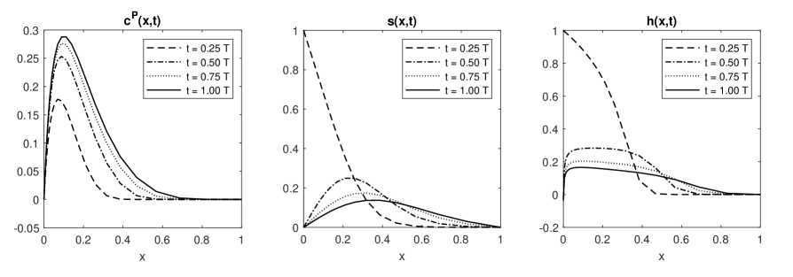
Figure 1: Numerical simulations for the system (5.1)–(5.6).

In order to illustrate the behavior of the solution, we propose a simplified 1D model with $\Omega=[0,1]$ described by the system

$$\rho^{W}s_{t}(x,t)-ks_{xx}(x,t) =\gamma m^{W}{h}s(1-s),$$ (5.1)

$$\rho^{H}h_{t}(x,t)-(\kappa sh_{x}-\rho^{H}hv)_{x} =-\gamma m^{H}{h}s(1-s),$$ (5.2)

for $x\in(0,L)$ and $t\in(0,T)$, with boundary conditions

$$ks_{x}(0,t) =\alpha(s(0,t)-\bar{s}(0,t)),$$ (5.3)

$$\kappa sh_{x}(0,t)-\rho^{H}h(0,t)v(0,t) =-\beta s(0,t)(\bar{h}(0,t)-h(0,t))^{+},$$ (5.4)

$$ks_{x}(1,t) =-\alpha s(1,t),$$ (5.5)

$$\kappa sh_{x}(1,t)-\rho^{H}h(1,t)v(1,t) =0,$$ (5.6)

with some constants $\alpha>0,\beta>0$. The data are chosen so as to model the following situation: We start with initial conditions $s^{0}=s^{\flat}$, $h^{0}=0$, and in the time interval $[0,T/4]$, we choose $\bar{s}=1$ and $\bar{h}=1$. This corresponds to the process of filling the structure with lime water solution until the time $t=T/4$. Then, at time $t=T/4$ we start the process of drying by switching $\bar{s}$ to $s^{\flat}$ and $\bar{h}$ to $0$. With these boundary data, we let the process run in the time interval $[T/4,T]$. Figure 1 shows the spatial distributions across the profile $x\in[0,1]$ at successive times $t=T/4,T/2,3T/4,T$. We have chosen a finer mesh size near the origin, where the solution exhibits higher gradients. High concentration of $CaCO_{3}$ near the active boundary $x=0$ exactly corresponds to the measurements shown, e. g., in [9, 25]. The parameters of our model cannot be easily taken from the available measurements, and a complicated identification procedure would be necessary. This is beyond the scope of this paper, whose purpose is to present a model to be validated by numerical simulations. For this qualitative study we have therefore chosen fictitious parameters with simple numerical values $\rho^{W}=\rho^{H}=m^{W}=m^{H}=\alpha=\beta=1,s^{\flat}=0,k=2\cdot 10^{-4},\kappa=10^{-3}$ and $\gamma=10^{-2}$. The final time $T$ is determined by the number of time steps which are necessary to reach approximate equilibrium. In fact, the question of asymptotic stabilization for large times will be a subject of a subsequent study.

References

• [1]
• [2] B. Albers, On adsorption and diffusion in porous media. ZAMM: Zeitschrift für Angewandte Mathematik und Mechanik 81 (10) (2001), 683–690.
• [3] B. Albers and P. Krejčí, Unsaturated porous media flow with thermomechanical interaction. Mathematical Methods in the Applied Sciences 39 (9) (2016), 2220–2238.
• [4] N. D. Alikakos, $L^{p}$ bounds of solutions of reaction diffusion equations. Communications Partial Differential Equations 4 (8) (1979), 827–868.
• [5] Z. P. Bažant and M. Z. Bazant, Theory of sorption hysteresis in nanoporous solids: Part i: Snap-through instabilities. Journal of the Mechanics and Physics of Solids 60 (9) (2012), 1644–1659.
• [6] M. Z. Bazant and Z. P. Bažant, Theory of sorption hysteresis in nanoporous solids: Part ii: molecular condensation. Journal of the Mechanics and Physics of Solids 60 (9) (2012), 1660–1675.
• [7] G. Borsoi, B. Lubelli, R. van Hees, R. Veiga, and A. Santos Silva, Evaluation of the effectiveness and compatibility of nanolime consolidants with improved properties. Construction and Building Materials 142 (2017), 385–394.
• [8] G. Borsoi, B. Lubelli, R. van Hees, R. Veiga, and A. Santos Silva, Optimization of nanolime solvent for the consolidation of coarse porous limestone. Applied Physics A 122 (2016), Art. No. 846.
• [9] G. Borsoi, B. Lubelli, R. van Hees, R. Veiga, and A. Santos Silva, Understanding the transport of nanolime consolidants within Maastricht limestone. Journal of Cultural Heritage 18 (2016), 242–249.
• [10] M. Böhm, J. Devinny, F. Jahani, and G. Rosen, On a moving-boundary system modeling corrosion in sewer pipes. Applied Mathematics and Computation 92 (2) (1998), 247–269.
• [11] G. Bretti, B. De Filippo, R. Natalini, S. Goidanich, M. Roveri, and L. Toniolo, Modelling the effects of protective treatments in porous materials. In: Mathematical Modeling in Cultural Heritage, Springer INdAM Series 41 (Eds. E. Bonetti, C. Cavaterra, R. Natalini, M. Solci), 2021, 73–83.
• [12] F. Clarelli, R. Natalini, C. Nitsch, and M. L. Santarelli, A mathematical model for consolidation of building stones. Applied and Industrial Mathematics in Italy III. Series on Advances in Mathematics for Applied Sciences 82 (2010), 232–243.
• [13] G. Creazza, A. Saetta, R. Scotta, R. Vitaliani, and E. Onate, Mathematical simulation of structural damage in historical buildings. Structural studies of historical buildings IV. Volume 1: architectural studies, materials and analysis, C. M. Publications, Ed. Southampton (1995), 111–118.
• [14] B. Detmann, Modeling chemical reactions in porous media: a review. Continuum Mechanics and Thermodynamics 33 (6) (2021), 2279–2300.
• [15] M. Drdácký, Z. Slížková, and G. Ziegenbalg, A nano approach to consolidation of degraded historic lime mortars. Journal of Nano Research 8 (2009), 13–22.
• [16] E. Gagliardo, Ulteriori proprietà di alcune classi di funzioni in più variabili. Ricerche di Matematica 8 (1959), 24–51.
• [17] D. Gawin, F. Pesavento and B. A. Schrefler, Modelling of hygro-thermal behaviour of concrete at high temperature with thermo-chemical and mechanical material degradation. Computer Methods in Applied Mechanics and Engineering 192 (13) (2003), 1731–1771.
• [18] J. Hoffmann, S. Kräutle, and P. Knabner, Existence and uniqueness of a global solution for reactive transport with mineral precipitation-dissolution and aquatic reactions in porous media. SIAM Journal on Mathematical Analysis 49 (6) (2017), 4812–4837.
• [19] Y. F. Houst and F. H. Wittmann. Influence of porosity and water content on the diffusivity of CO2 and O2 through hydrated cement paste. Cement and Concrete Research 24 (6) (1994), 1165–1176.
• [20] J.-L. Lions, Quelques méthodes de résolution des problèmes aux limites non linéaires. Dunod; Gauthier-Villars, Paris 1969.
• [21] M. J. Mosquera, J. Pozo, and L. Esquivias, Stress during drying of two stone consolidants applied in monumental conservation. Journal of Sol-Gel Science and Technology 26 (2003), 1227–1231.
• [22] M. J. Mosquera, D. M. de los Santos, and A. Montes, Producing new stone consolidants for the conservation of monumental stones. In: Materials Research Society Symposium Proceedings 852 (2005), 81–87.
• [23] A. Muntean, M. Böhm, and J. Kropp, Moving carbonation fronts in concrete: A moving-sharp-interface approach. Chemical Engineering Science 66 (3) (2011), 538–547.
• [24] J. Nečas, Les méthodes directes en théorie des équations elliptiques, Academia, Prague, 1967.
• [25] K. Niedoba, Z. Slížková, D. Frankeová, C. L. Nunes, and I. Jandejsek, Modifying the consolidation depth of nanolime on Maastricht limestone. Construction and Building Materials 133 (2017), 51–56.
• [26] L. Nirenberg, On elliptic partial differential equations. Ann. Scuola Norm. Sup. Pisa 13 (2) (1959), 115–162.
• [27] S. Papatzani and E. Dimitrakakis, A review of the assessment tools for the efficiency of nanolime calcareous stone consolidant products for historic structures. Buildings 9 (11) (2019), Article No. 235.
• [28] J. S. Pozo-Antonio, J. Otero, P. Alonso, and X. Mas i Barberà, Nanolime- and nanosilica-based consolidants applied on heated granite and limestone: Effectiveness and durability. Construction and Building Materials 201 (2019), 852–870.
• [29] M. Renardy and R. Rogers, An Introduction to Partial Differential Equations. Texts in Applied Mathematics 13. New York: Springer-Verlag, 2004.
• [30] H. Roques and A. Girou, Kinetics of the formation conditions of carbonate tartars. Water Research 8 (11) (1974), 907–920.
• [31] A. V. Saetta, B. A. Schrefler and R. V. Vitaliani, The carbonation of concrete and the mechanism of moisture, heat and carbon dioxide flow through porous materials. Cement and Concrete Research 23 (4) (1993), 761–772.
• [32] A. V. Saetta, B. A. Schrefler and R. V. Vitaliani, $2$-D model for carbonation and moisture/heat flow in porous materials. Cement and Concrete Research 25 (8) (1995), 1703–1712.
• [33] G. W. Scherer and E. Sassoni, Mineral consolidants, In: I. Rörig-Dalgaard and I. Ioannou (Eds), Proceedings of the International RILEM Conference Materials, Systems and Structures in Civil Engineering 2016, 1–10.
• [34] R. Schulz, N. Ray, F. Frank, H. S. Mahato, and P. Knabner, Strong solvability up to clogging of an effective diffusion-precipitation model in an evolving porous medium. European Journal of Applied Mathematics 28 (2) (2017), 179–207.
• [35] R. Ševčík, A. Viani, D. Machová, G. Lanzafame, L. Mancini, and M.-S. Appavou, Synthetic calcium carbonate improves the effectiveness of treatments with nanolime to contrast decay in highly porous limestone. Scientific Reports 9 (2019), Article No.  15278.
• [36] K. van Balen and D. van Gemert, Modelling lime mortar carbonation. Materials and Structures 27 (1994), 393–398.
• [37] A. J. Vromans, A. Muntean and A. A. F. van de Ven, A mixture theory-based concrete corrosion model coupling chemical reactions, diffusion and mechanics. Pacific Journal of Mathematics for Industry 10 (2018), Article No. 5.
• [38] N. M. Zouridakis, I. G. Economou, K. P. Tzevelekos and E. S. Kikkinides, Investigation of the physicochemical characteristics of ancient mortars by static and dynamic studies. Cement and Concrete Research 30 (7) (2000), 1151–1155.