Neuronal avalanches and critical dynamics of brain waves

Abstract

Analytical expressions for scaling of brain wave spectra derived from the general nonlinear wave Hamiltonian form show excellent agreement with experimental ”neuronal avalanche” data. The theory of the weakly evanescent nonlinear brain wave dynamics (Galinsky and Frank, 2020a; *Galinsky:2020b) reveals the underlying collective processes hidden behind the phenomenological statistical description of the neuronal avalanches and connects together the whole range of brain activity states, from oscillatory wave-like modes, to neuronal avalanches, to incoherent spiking, showing that the neuronal avalanches are just the manifestation of the different nonlinear side of wave processes abundant in cortical tissue. In a more broad way these results show that a system of wave modes interacting through all possible combinations of the third order nonlinear terms described by a general wave Hamiltonian necessarily produces anharmonic wave modes with temporal and spatial scaling properties that follow scale free power laws. To the best of our knowledge this was never reported in the physical literature and may be applicable to many physical systems that involve wave processes and not just to neuronal avalanches.

The standard view of brain electromagnetic activity classifies this activity into two significant but essentially independent classes. The first class includes a variety of the oscillatory and wave-like patterns that show relatively high level of coherence across a wide range of spatial and temporal scales (Buzsaki, 2006). The second class focusses on the asynchronous, seemingly incoherent spiking activity at scales of a single neuron and often uses various ad hoc neuron models (Hodgkin and Huxley, 1952; *pmid19431309; *Nagumo1962; *pmid7260316; *pmid18244602) to describe this activity. Linking these two seemingly disparate classes to explain the emergence of oscillatory rhythms from incoherent activity is essential to understanding brain function and is typically posed in the form using the construct of networks of incoherently spiking neurons (Gerstner et al., 2014; *pmid33192427; *pmid33288909).

Coherent macroscopic behavior arising from seemingly incoherent microscopic processes naturally suggests the influence of critical phenomena, a potential model from brain activity that was bolstered by the experimental discovery of the “neuronal avalanches”(Beggs and Plenz, 2003; *pmid15175392) where both spatial and temporal distributions of spontaneous propagating neuronal activity in 2D cortex slices were shown to follow scale-free power laws. This discovery has generated significant interest in the role and the importance of criticality in brain activity (Friedman et al., 2012; *2010NatPh...6..744Cl; *pmid22701101; *pmid25009473; *pmid32503982; *pmid31172737), especially for transmitting or processing information (Fosque et al., 2021).

Although the precise neuronal mechanisms leading to the observed scale-free avalanche behavior is still uncertain after almost 20 years since their discovery, the commonly agreed upon paradigm is that this collective neuronal avalanche activity represents a unique and specialized pattern of brain activity that exists somewhere between the oscillatory, wave-like coherent activity and the asynchronous and incoherent spiking. Central to this claim of neuronal avalanches as a unique brain phenomena is that they do not show either wave-like propagation or synchrony at short scales, and thus constitute a new mode of network activity (Beggs and Plenz, 2003; *pmid15175392) that can be phenomenologically described using the ideas of the self-organized criticality (Bak et al., 1987; *PhysRevA.38.364), and extended to the mean-field theory of the self-organized branching processes (SOBP) (Zapperi et al., 1995; *PhysRevE.54.2483; *pmid12513377).

However, despite the success of the SOBP theory in describing neuronal avalanche statistical properties, i.e., replicating the power law exponents based on the criticality considerations, the SOBP theory provides no explanation about the physical mechanisms of the critical behavior and its relationship to the development of the observed collective neuronal “avalanche” behavior. Because similar statistics can result from several mechanisms other than critical dynamics (Bédard et al., 2006; *pmid20161798; *pmid28208383), it is essential to have a physical model that explains the relationship between the statistical properties and the existence, if any, of critical neural phenomena arising from the actual collective behavior of neuronal populations. While it is generally accepted in that some form of critical phenomena is at work, this has led to the presupposition of ad hoc descriptive models (Robinson et al., 1997; *pmid28505725; *pmid12005890; *SantoE1356) that exhibit critical behavior, but provide no insight into the actual physical mechanisms that might produce such critical dynamics.

In this Letter we show that our recently described theory of weakly evanescent brain waves (WETCOW) originally developed in (Galinsky and Frank, 2020a; *Galinsky:2020b) and then reformulated in a general Hamiltonian framework (Galinsky and Frank, 2021) provides a physical theory, based on the propagation of electromagnetic fields through the highly complex geometry of inhomogeneous and anisotropic domain of real brain tissues, that explains the broad range of observed seemingly disparate brain wave characteristics. This theory produces a set of nonlinear equations for both the temporal and spatial evolution of brain wave modes that includes all possible nonlinear interaction between propagating modes at multiple spatial and temporal scales and degrees of nonlinearity. This theory bridges the gap between the two seemingly unrelated spiking and wave ’camps’ as the generated wave dynamics includes the complete spectra of brain activity ranging from incoherent asynchronous spatial or temporal spiking events, to coherent wave-like propagating modes in either temporal or spatial domains, to collectively synchronized spiking of multiple temporal or spatial modes. Consequently, we demonstrate that the origin of these ’avalanche’ properties emerges directly from the same theory that produces this wide range of activity and does not require one to posit the existence of either new brain activity states, nor construct analogies between brain activity and ad hoc generic ’sandpile’ models.

Following (Galinsky and Frank, 2021) we begin with a nonlinear Hamiltonian form for an anharmonic wave mode

$$H^{s}(a,a^{\dagger}) =\Gamma aa^{\dagger}\!+aa^{\dagger}\!\left[\beta_{a}a+\beta_{a^{\dagger}}a^{\dagger}\!-2\alpha\left(aa^{\dagger}\right)^{1/2}\right]$$ (1)

where $a$ is a complex wave amplitude and $a^{\dagger}$ is its conjugate. The amplitude $a$ denotes either temporal $a_{k}(t)$ or spatial $a_{\omega}(x)$ wave mode amplitudes that are related to the spatiotemporal wave field $\psi(x,t)$ through a Fourier integral expansions

$$a_{k}(t)=\frac{1}{2\pi}\int\limits_{-\infty}^{\infty}\psi(x,t)e^{-i\left(kx+\omega_{k}t\right)}dx,$$ (2)

$$a_{\omega}(x)=\frac{1}{2\pi}\int\limits_{-\infty}^{\infty}\psi(x,t)e^{-i\left(k_{\omega}x+\omega t\right)}dt,$$ (3)

where for the sake of clarity we use one dimensional scalar expressions for spatial variables $x$ and $k$, but it can be easily generalized for the multi dimensional wave propagation as well. The frequency $\omega$ and the wave number $k$ of the wave modes satisfy dispersion relation $D(\omega,k)=0$, and $\omega_{k}$ and $k_{\omega}$ denote the frequency and the wave number roots of the dispersion relation (the structure of the dispersion relation and its connection to the brain tissue properties has been discussed in (Galinsky and Frank, 2020a)). The multiple temporal $a_{k}(t)$ or spatial $a_{\omega}(x)$ wave mode amplitudes can be used to define the time dependent wave number energy spectral density $\P_{k}(t)$ or the position dependent frequency energy spectral density $\P_{\omega}(x)$ for the spatiotemporal wave field $\psi(x,t)$ as

$$\P_{k}(t)=|a_{k}(t)|^{2},\qquad\P_{\omega}(x)=|a_{\omega}(x)|^{2},$$ (4)

or alternatively we can add additional length or time normalizations to convert those quantities to power spectral densities instead.

The first term $\Gamma aa^{\dagger}$ in 1 denotes the harmonic (quadratic) part of the Hamiltonian with either the complex valued frequency $\Gamma=i\omega+\gamma$ or the wave number $\Gamma=ik+\lambda$ that both include a pure oscillatory parts ($\omega$ or $k$) and possible weakly excitation or damping rates, either temporal $\gamma$ or spatial $\lambda$. The second anharmonic term is cubic in the lowest order of nonlinearity and describes the interactions between various propagating and nonpropagating wave modes, where $\alpha$, $\beta_{a}$ and $\beta_{a^{\dagger}}$ are the complex valued strengths of those different nonlinear processes.

An equation for the nonlinear oscillatory amplitude $a$ then can be expressed as a derivative of the Hamiltonian form

$$\frac{d{a}}{d{t}}=\frac{\partial{H^{s}}}{\partial{a^{\dagger}}}\equiv\Gamma a+\beta_{a^{\dagger}}aa^{\dagger}+\beta_{a}a^{2}-\alpha a(aa^{\dagger})^{1/2},$$ (5)

after removing the constants with a substitution of $\beta_{a^{\dagger}}=1/2\tilde{\beta}_{a^{\dagger}}$ and $\alpha=1/3\tilde{\alpha}$ and dropping the tilde. We note that although 5 is an equation for the temporal evolution, the spatial evolution of the mode amplitudes $a_{\omega}(x)$ can be described by a similar equation substituting temporal variables by their spatial counterparts, i.e., $(t,\omega,\gamma)\rightarrow(x,k,\lambda)$.

Splitting 5 into an amplitude/phase pair of equations using $a=Ae^{i\phi}$, assuming $\beta_{a}=\tilde{\beta_{a}}e^{-i\delta_{a}}$, $\beta_{a^{\dagger}}=\tilde{\beta}_{a^{\dagger}}e^{i\delta_{a^{\dagger}}}$, and scaling the variables as

$$A=\gamma\tilde{A},\quad t=\frac{\tau}{\gamma},\quad\omega=\tilde{\omega}\gamma,$$ (6)

gives the set of equations

$$\frac{d{\tilde{A}}}{d{\tau}} =\tilde{A}+\tilde{A}^{2}\left(\beta_{a^{\dagger}}\cos\Omega_{a^{\dagger}}+\beta_{a}\cos\Omega_{a}-\alpha\right)$$ (7)

$$\frac{d{\phi}}{d{\tau}} =\tilde{\omega}+\tilde{A}\left(-\beta_{a^{\dagger}}\sin\Omega_{a^{\dagger}}+\beta_{a}\sin\Omega_{a}\right)\$$ (8)

where $\Omega_{a}\equiv\phi-\delta_{a}$, $\Omega_{a^{\dagger}}\equiv\phi-\delta_{a^{\dagger}}$.

These equations can further be cast into a more compact form as

$$\frac{d{\tilde{A}}}{d{\tau}} =\tilde{A}+\tilde{A}^{2}\left[R_{a}\cos{(\phi-\Phi)}-\alpha\right],$$ (9)

$$\frac{d{\phi}}{d{\tau}} =\tilde{\omega}+\tilde{A}R_{\phi}\cos{\phi},$$ (10)

where

$$R_{a} =\sqrt{X_{a}^{2}+Y_{a}^{2}},\quad R_{\phi}=\sqrt{X_{\phi}^{2}+Y_{\phi}^{2}},$$ (11)

$$\Phi_{a} =\arctan{\frac{Y_{a}}{X_{a}}},\quad\Phi_{\phi}=\arctan{\frac{Y_{\phi}}{X_{\phi}}},$$ (12)

$$\Phi =\Phi_{a}-\Phi_{\phi},$$ (13)

and

$$X_{a} =\phantom{-}\beta_{a^{\dagger}}\cos{\delta_{a^{\dagger}}}+\beta_{a}\cos{\delta_{a}},$$

$$Y_{a} =\phantom{-}\beta_{a^{\dagger}}\sin{\delta_{a^{\dagger}}}+\beta_{a}\sin{\delta_{a}},$$

$$X_{\phi} =\phantom{-}\beta_{a^{\dagger}}\sin{\delta_{a^{\dagger}}}-\beta_{a}\sin{\delta_{a}},$$

$$Y_{\phi} =-\beta_{a^{\dagger}}\cos{\delta_{a^{\dagger}}}+\beta_{a}\cos{\delta_{a}},$$

An equilibrium (i.e., $d\tilde{A}/d\tau=d\phi/d\tau=0$) solution of 9 and 10 can be found from

$$-\frac{R_{\phi}}{\tilde{\omega}}\cos{\phi}+R_{a}\cos{(\phi-\Phi)}-\alpha=0,$$ (14)

as $\phi_{e}=\phi_{0}\equiv$ const and $\tilde{A}_{e}=\tilde{\omega}/R_{\phi}\cos{\phi_{0}}\equiv$ const. This shows that for $\alpha>R_{a}$ there exist critical values of $\tilde{\omega}$ and $A_{e}$, such that

$$\tilde{\omega}_{c} =\frac{R_{\phi}}{\alpha+R_{a}\cos{\Phi}},\quad\tilde{A}_{c}=\tilde{\omega}_{c}/R_{\phi}$$ (15)

which can also be expressed in terms of critical value of one of the unscaled variables, either $\omega$ or $\gamma$

$$\omega_{c} =\gamma\tilde{\omega}_{c},\quad\mathrm{or}\quad\gamma_{c}=\frac{\omega}{\tilde{\omega}_{c}},$$ (16)

This equilibrium solution provides the locus of the bifurcation point at where the nonlinear spiking oscillations occur (as was shown both in (Galinsky and Frank, 2020a; *Galinsky:2020b) and in (Galinsky and Frank, 2021)).

The effective period of spiking $\mathscr{T}_{s}$ (or its inverse – either the firing rate 1/$\mathscr{T}_{s}$ or the effective firing frequency $2\pi/\mathscr{T}_{s}$) can be estimated from 10 by substituting $\tilde{A}_{c}$ for $\tilde{A}$ (assuming that the change of amplitude $\tilde{A}$ is slower than the change of the phase $\phi$) as

$$\mathscr{T}_{s} =\int\limits_{0}^{2\pi}\frac{d\phi}{\tilde{\omega}+\tilde{\omega}_{c}\cos{\phi}}=\frac{2\pi}{\sqrt{\tilde{\omega}^{2}-\tilde{\omega}_{c}^{2}}},$$ (17)

giving the unscaled effective spiking period $T_{s}$ and the effective firing frequency $\omega_{s}$

$$T_{s} =\frac{\mathscr{T}_{s}}{\gamma}=\frac{2\pi}{\omega\sqrt{1-{\gamma^{2}}/{\gamma_{c}^{2}}}}=\frac{2\pi}{\omega\sqrt{1-\omega_{c}^{2}/\omega^{2}}},$$ (18)

$$\omega_{s} =\frac{2\pi}{T_{s}}=\omega\sqrt{1-\omega_{c}^{2}/\omega^{2}},$$ (19)

with the periodic amplitude $\tilde{A}$ reaching the maximum $\tilde{A}_{max}=1/(\alpha-R_{a})$ and the minimum $\tilde{A}_{min}=1/(\alpha+R_{a})$ for $d\tilde{A}/d\tau=0$ when $\phi=\Phi$ and $\phi=\Phi+\pi$ respectively.

The expressions 18 and 19 are more general than typically used expressions for the scaling exponent in the close vicinity $|\gamma-\gamma_{c}|\ll\gamma_{c}$ of the critical point (Kuramoto, 2013; *pmid10057530; *pmid10058476). They allow recovery of the correct $T$ limits both at $\gamma\rightarrow\gamma_{c}$ with the familiar $T\sim 1/\sqrt{\gamma_{c}-\gamma}$ scaling and at $\gamma\sim 0$ with the period $T$ approaching $T_{0}$ as $T\sim T_{0}+O(\gamma^{2})\equiv 2\pi/\omega+O(\gamma^{2})$, where $T_{0}$ is the period of linear wave oscillations with the frequency $\omega$. In the intermediate range $0<\gamma<\gamma_{c}$ the expressions 18 and 19 show reasonable agreement (Fig. ​​​ 1) with peak–to–peak period/frequency estimates from direct simulations of the system 7 and 8.

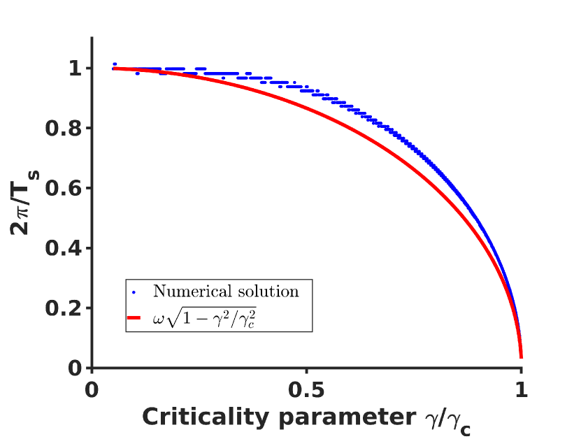
Figure 1: Comparison of the analytical expression 19 for the effective spiking frequency $\omega_{s}=2\pi/T_{s}$ (red) and the frequency estimated from numerical solution of 9 and 10 (blue) as a function of the criticality parameter $\gamma/\gamma_{c}$. In the numerical solution only $\gamma$ was varied and the remaining parameters were the same as parameters reported in (Galinsky and Frank, 2021).

Taking into account that the initial phase of spiking solutions of 9 and 10 is a random variable uniformly distributed on $[0,2\pi]$ interval, the probability that a spike (either positive or the more frequently experimentally reported negative (Beggs and Plenz, 2003; *pmid15175392)) with duration width $\delta t_{s}$ and with the total period between the spikes ($T_{s}$) will be detected is simply $\delta t_{s}/T_{s}$ – where the distance between spikes is determined as the time interval needed for 2$\pi$ radian phase change, that is the effective spiking period $T_{s}$. Assuming initially that the spike width $\delta t_{s}$ does not change when approaching the critical point $\omega_{c}$, $\delta t_{s}$ can be approximated by some fixed fraction of the linear wave period, i.e., $\delta t_{s}\sim\pi/\omega$, that gives for the probability density

$${P}_{k}^{\{\omega\}}(\omega)\sim\omega^{-1}\sqrt{\omega^{2}/\omega_{c}^{2}-1},$$ (20)

for every wave mode with the wavenumber $k$. It should be noted that the probability density ${P}_{k}^{\{\omega\}}(\omega)$ has no relation and should not be confused with the frequency energy spectral density $\P_{\omega}(x)$ (or with the power spectral density).

Transforming the frequency dependence of the wavenumber spectra ${P}_{k}^{\{\omega\}}(\omega)$ to the temporal domain ($T=2\pi/\omega$, $T_{c}=2\pi/\omega_{c}$)

$$\int\limits_{\omega_{c}}^{\infty}{P}_{k}^{\{\omega\}}(\omega)d\omega=\int\limits_{0}^{T_{c}}{P}_{k}^{\{\omega\}}\left(\frac{2\pi}{T}\right)\frac{2\pi}{T^{2}}dT=\int\limits_{0}^{T_{c}}{P}_{k}^{\{T\}}(T)dT,$$ (21)

gives for the temporal probability density ${P}_{k}^{\{T\}}(T)$

$${P}_{k}^{\{T\}}(T)\sim T^{-2}\sqrt{1-T^{2}/T_{c}^{2}},$$ (22)

hence the scaling of the temporal probability density ${P}_{k}^{\{T\}}$ follows the power law with -2 exponent with additional $\sqrt{1-T/T_{c}}$ falloff in close vicinity of the critical point in agreement with temporal scaling of neuronal avalanches reported in (Beggs and Plenz, 2003; *pmid15175392).

The above single wave mode analysis shows that the probability density ${P}_{k}^{\{T\}}$ for any arbitrary selected wave mode $k$ with arbitrary chosen threshold follows power law distribution with -2 exponent, therefore, a mixture of multiple wave modes that enters into the spatiotemporal wave field $\psi(x,t)$ with different amplitudes and different thresholds will again show nothing more than the same power law distribution.

Due to the reciprocity of the temporal and spatial representations of the Hamiltonian form 1 equations for the spatial wave amplitude have the same form as the temporal equations 9 and 10

$$\frac{d{\tilde{A}}}{d{\xi}} =\tilde{A}+\tilde{A}^{2}\left[R_{a}\cos{(\phi-\Phi)}-\alpha\right],$$ (23)

$$\frac{d{\phi}}{d{\xi}} =\tilde{k}+\tilde{A}R_{\phi}\cos{\phi},$$ (24)

under similar scaling (the spatial equivalent of 6) of the wave amplitude, the coordinate, and the wave number

$$A=\lambda\tilde{A},\quad x=\frac{\xi}{\lambda},\quad k=\tilde{k}\lambda.$$ (25)

In the spatial domain, this leads to the critical parameters $\tilde{A}_{c}$ and $\tilde{k}_{c}$

$$\tilde{k}_{c} =\frac{R_{\phi}}{\alpha+R_{a}\cos{\Phi}},\quad\tilde{A}_{c}=\tilde{k}_{c}/R_{\phi}.$$ (26)

Although our simple one dimensional scaling estimates do not take into account the intrinsic spatial scales of the brain, e.g., cortex radius of curvature, cortical thickness, etc., nevertheless, even in this simplified form the similarity between spatial and temporal nonlinear equations suggests that the nonlinear spatial wave behavior will generally look like spiking in the spatial domain where some localized regions of activity are separated by areas that are relatively signal free and this separation will increase near the critical point. Exactly this behavior was reported in the original experimental studies of the neuronal avalanches (Beggs and Plenz, 2003; *pmid15175392), where it was stated that the analysis of the contiguity index revealed that activity detected at one electrode is most often skipped over the nearest neighbors, but this experimental observation of near critical nonlinear waves was instead presented as the indicator that the activity propagation is not wave-like. The effects of the intrinsic spatial scales of the brain will certainly affect the details of the spatial critical wave dynamics and so their inclusion will be important for more completely characterizing the details of brain criticality and will be the focus of future investigations.

Using the spatial equations 23 and 24 similar scaling results can be obtained for the wave number $k$ and the linear spatial dimension $L$ probabilities for every wave mode with the frequency $\omega$ as

$${P}_{\omega}^{\{k\}}(k) \sim k^{-1}\sqrt{k^{2}/k_{c}^{2}-1},$$ (27)

$${P}_{\omega}^{\{L\}}(L) \sim L^{-2}\sqrt{1-L^{2}/L_{c}^{2}},$$ (28)

where $L$ is the linear spatial scale related to the wave number as $k=2\pi/L$.

The linear spatial dimension of the avalanche $L$ is related to its area $S$ on a 2 dimensional surface as $L=\sqrt{S}$, hence

$$\int\limits_{0}^{L_{c}}{P}_{\omega}^{\{L\}}(L)dL=\int\limits_{0}^{S_{c}}\frac{{P}_{\omega}^{\{L\}}\left(\sqrt{S}\right)}{2\sqrt{S}}dS=\int\limits_{0}^{S_{c}}{P}_{\omega}^{\{S\}}(S)dS,$$ (29)

$${P}_{\omega}^{\{S\}}(S)\sim S^{-3/2}\sqrt{1-S/S_{c}},$$ (30)

hence the spatial probability scaling for the size $S$ follows the power law with -3/2 exponent again with additional $\sqrt{1-S/S_{c}}$ falloff in close vicinity of the critical point, that is also in agreement with experimentally reported spatial scaling of neuronal avalanches (Beggs and Plenz, 2003; *pmid15175392). We would like to mention that the nonlinear anharmonic oscillations described by the 9 and 10 only exists for frequencies and wave numbers that are above the critical frequency $\omega_{c}$ or the critical wave number $k_{c}$ values that define maximal possible temporal $T_{c}$ or spatial $L_{c}$ scales of the nonlinear oscillations. If the finite system sizes are below those maximal values the cutoffs will be defined by the system scales.

The assumption of the fixed spike duration $\delta t_{s}$ used in 20 and 22 (or the spike length for spatial spiking in 27 and 28) can be improved by estimating the scaling of the spike width as a function of the criticality parameter from the amplitude equation (we will use the temporal form of the equation 9 but the spatial analysis with equation 23 is exactly the same).

Dividing equation 9 by $\tilde{A}$ and taking an integral around some area in the vicinity of the amplitude peak $\tilde{A}_{max}$ we can write

$$\int\limits_{\tilde{A}_{-}}^{\tilde{A}_{+}}\frac{1}{\tilde{A}}d\tilde{A}=\int\limits_{\tau_{-}}^{\tau_{+}}d\tau+\int\limits_{\Phi_{-}}^{\Phi_{+}}\frac{\tilde{\omega}_{c}}{R_{\phi}}\frac{R_{a}\cos{(\phi-\Phi)}-\alpha}{\tilde{\omega}+\tilde{\omega}_{c}\cos{\phi}}d\phi,$$ (31)

where $\tau_{\pm}=\tau_{max}\pm\delta\tau$, and $\tau_{max}$ is the location of spiking peak. Neglecting the spike shape asymmetries, i.e., assuming that $\tau_{\pm}$ correspond to symmetric changes in both the amplitudes $\tilde{A}_{\pm}=\tilde{A}(\tau_{\pm})=\tilde{A}_{max}-\delta\tilde{A}$, and the phases $\Phi_{\pm}=\Phi(\tau_{\pm})=\Phi\pm\delta\Phi$, we can then estimate the spike duration $\delta t_{s}\equiv(\tau_{+}-\tau_{-})/\gamma$ as

$$\delta t_{s}=\frac{1}{\gamma}\int\limits_{\Phi-\delta\Phi}^{\Phi+\delta\Phi}\frac{1-R(\cos(\Phi)+\cos{(\phi-\Phi))}}{\tilde{\omega}+\tilde{\omega}_{c}\cos{\phi}}d\phi,$$ (32)

where, similar to the spiking period estimation in 18, we again assume that the main contribution comes from the change of the oscillation phase, hence $\tilde{A}_{c}$ can be substituted for $\tilde{A}$. For $\delta\Phi$ some fixed value that is smaller or around a quarter of the period (i.e., $\delta\Phi\lesssim\pi/2$) can be chosen, and $R=\tilde{\omega}_{c}R_{a}/R_{\phi}$.

An expression 32 can be evaluated in closed form but we do not include it here and instead plotted the final spatial probability density spectra ${P}(S/S_{c})$, similarly obtained from the expression for $\delta l_{s}/L_{s}$ again substituting $L=\sqrt{S}$ and $dL=dS/(2\sqrt{S})$, for several values of the phase shift $\Phi$ (Fig. ​​​ 2). The spectra clearly show again the same power law dependence with -3/2 exponent as was reported in (Beggs and Plenz, 2003; *pmid15175392) followed by a steep falloff sufficiently close to the critical point. What is interesting, however, is that the spectra for $\Phi=\pi/2$ (and this is the phase shift value used for spiking solutions reported in (Galinsky and Frank, 2020a; *Galinsky:2020b; Galinsky and Frank, 2021)) recover even the fine structure of the scaling and clearly show the small bump at the end of the scale free part of the spectra where the local probability deflects from the initial -3/2 power exponent and flattens first before turning in to the steep falloff. These small bumps are evident in all experimental spectra (Beggs and Plenz, 2003; *pmid15175392) shown on the insert in Fig. ​​​ 2.

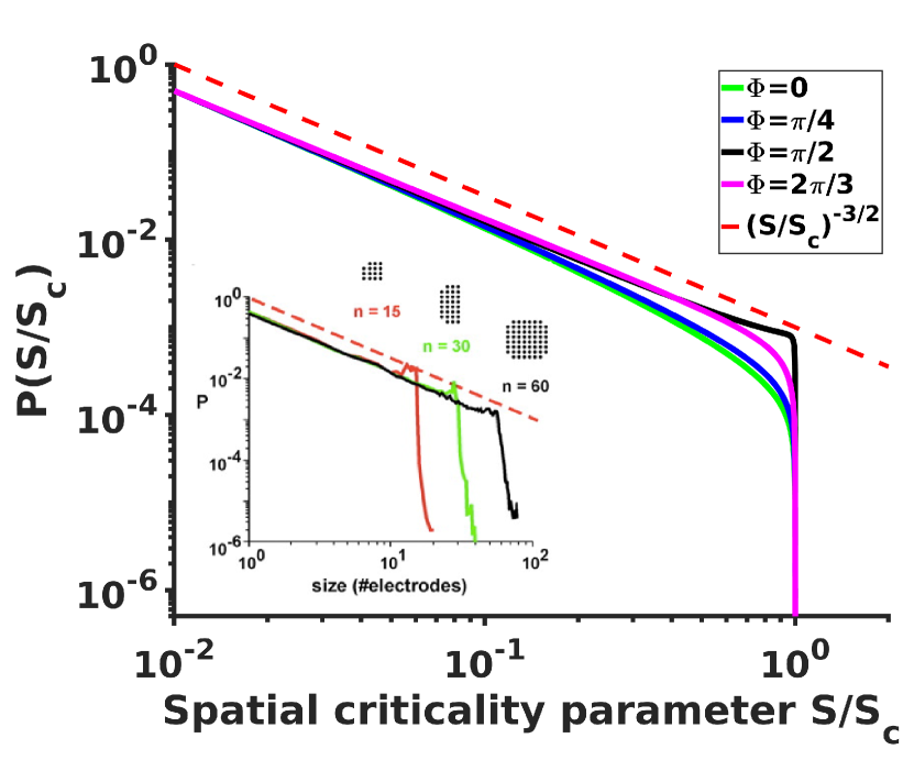
Figure 2: Analytical probability density spectra as a function of brain waves criticality parameter $S/S_{c}$ show excellent agreement with the experimental avalanche data (insert, from (Beggs and Plenz, 2003; *pmid15175392)) reproducing not only the overall shape of the spectra with the -3/2 power exponent at the initial scale free part of the spectra and the steep falling edge in the vicinity of the critical point, but also reproduce the fine details such as the small bump-like flattening of the spectra at the transition from -3/2 leg to the steep falling edge that is clearly evident in experimental spectra.

In summary, in this Letter we have presented an analysis of temporal and spatial probability density spectra that are generated due to the critical dynamics of the nonlinear weakly evanescent cortical wave (WETCOW) modes (Galinsky and Frank, 2020a; *Galinsky:2020b). The Hamiltonian framework developed for these WETCOW modes in (Galinsky and Frank, 2021) is advantageous in that it explicitly uncovers the reciprocity of the temporal and the spatial dynamics of the evolutionary equations. Therefore, in the nonlinear regime sufficiently close to the critical point the spatial behavior of the wave modes displays features similar to the properties of their nonlinear temporal dynamics that can be described as spatial domain spiking, with localized regions of wave activity separated by quiescent areas, with this spatial spiking intermittence increasing near the critical point. Similar spatial behavior was observed experimentally in neuronal avalanches, when activity detected at one electrode was typically skipped over the nearest neighbors. This was interpreted as evidence that avalanche spatial intermittency is not wave-like in nature (Beggs and Plenz, 2003; *pmid15175392). Our results demonstrate the contrary, however: the spatial patterns are the direct result of nonlinear interactions of weakly evanescent cortical waves.

Both temporal and spatial scaling expressions analytically estimated from the nonlinear amplitude/phase evolutionary equations show excellent agreement with the experimental neuronal avalanche probability spectra reproducing not only the general average power law exponent values and falloffs in the vicinity of the critical point, but also finding some very subtle but nevertheless clearly experimentally evident fine details, like bumps in the transition region at the edge of the scale free part of the probability spectra.

The brain wave model thus uncovers the physical processes behind the emergence of avalanches that were hidden for almost 20 years since their discovery and demonstrates that the power scaling property of the neuronal avalanches can be explained by the same criticality that is responsible for spiking events in either space or time and is a consequence of a nonlinear interaction of weakly evanescent transverse cortical waves (WETCOWs, (Galinsky and Frank, 2020a; *Galinsky:2020b)). The origin of these ’avalanche’ properties emerges directly from the same theory that produces the wide range of oscillatory, synchronized, and wave-like network states, and does not require one to posit the existence of either new brain activity states, nor construct analogies between brain activity and ad hoc generic ’sandpile’ models (Gal, ).

In a more general way these results may be applicable not only to neuronal avalanches but to many other physical systems that involve wave processes as they show that a system of wave modes interacting through all possible combinations of the third order nonlinear terms described by a general wave Hamiltonian necessarily produces anharmonic wave modes with temporal and spatial scaling properties that follow scale free power laws.