“Will You Find These Shortcuts?”
A Protocol for Evaluating the Faithfulness
of Input Salience Methods for Text Classification

Abstract

Feature attribution a.k.a. input salience methods which assign an importance score to a feature are abundant but may produce surprisingly different results for the same model on the same input. While differences are expected if disparate definitions of importance are assumed, most methods claim to provide faithful attributions and point at the features most relevant for a model’s prediction. Existing work on faithfulness evaluation is not conclusive and does not provide a clear answer as to how different methods are to be compared. Focusing on text classification and the model debugging scenario, our main contribution is a protocol for faithfulness evaluation that makes use of partially synthetic data to obtain ground truth for feature importance ranking. Following the protocol, we do an in-depth analysis of four standard salience method classes on a range of datasets and lexical shortcuts for BERT and LSTM models. We demonstrate that some of the most popular method configurations provide poor results even for simple shortcuts while a method judged to be too simplistic works remarkably well for BERT.

1 Introduction

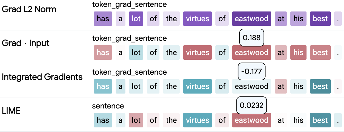
Figure 1: Salience maps produced by four common methods on a sentiment classification example (SST2) for a BERT model. The same token (eastwood) is assigned the highest (Grad-L2), the lowest (GxI, LIME) and a mid-range (IG) importance score (color intensity indicates salience; blue and purple stand for positive, red stands for negative weights). A developer investigating a hypothesis about specific named entities being associated with the label would probably be unsure as to whether the example provides support for or against the hypothesis.

A prominent class of explainability techniques assign salience scores to the input features, which reflect the importance of the features to the model’s decision. When applied to text classifiers those methods produce highlights over the input (sub)words. Interestingly, different methods may produce surprisingly dissimilar highlights. Figure 1 shows this using the Language Interpretability Tool (Tenney et al., 2020). So a natural question is: which method should one use? While a method whose highlights happen to look plausible may facilitate a task like text annotation Pavlopoulos et al. (2017); Strout et al. (2019); Schmidt and Biessmann (2019), many salience methods seem to be motivated by the debugging scenario where faithfulness to the model’s reasoning is a requirement Jacovi and Goldberg (2020). Indeed, known success stories from input salience methods in domains other than language are similar in that they teach us a lesson of not trusting a classifier based on its stellar performance on a standard test set. In the medical domain, for example, heatmaps over images helped uncover so-called shortcuts Geirhos et al. (2020) or spurious correlations between data artifacts like doctor marks or tags and the predicted disease (Codella et al., 2019; Sundararajan et al., 2019; Winkler et al., 2019, inter alia).

Spurious correlations plague NLP models too Gururangan et al. (2018); Poliak et al. (2018); Belinkov et al. (2019); Rosenman et al. (2020); Geva et al. (2019); McCoy et al. (2019) – notorious examples are the tendencies of NLI classifiers to overrely on negation or identity words when predicting contradiction and toxicity, respectively McCoy et al. (2019); Dixon et al. (2018). Importantly, shortcuts can comprise multiple tokens. For example, Kaushik et al. (2020) and Ross et al. (2021) demonstrated that BERT sentiment classifiers trained on IMDB Maas et al. (2011) learn to largely ignore the review text when patterns like ‘3 out of 10’ or ‘7 / 10’ are present – that is, when the numeric rating is made explicit in the text. Making such lexical shortcuts apparent to the developer is thus a strong use case for faithful input salience methods which would then indeed help them improve both the model and the data.

Figure 2: The proposed protocol to obtain ground truth importance rankings.

How can we know if a method consistently places the shortcut tokens on top of its salience rankings? Evaluating this is challenging, because we usually do not know the shortcut in advance and the model parameter space is large. Moreover, we don’t have an inherently interpretable view into the predictions of common black-box neural models. Glass-box models with explicit mediating factors (Camburu et al., 2019; Hao, 2020) are not widely used or are synthetic, and model-native structures such as attention have been shown to have weak predictive power (Bastings and Filippova, 2020). Alternatively, one can make strong assumptions about what a ground truth should be like and compare salience rankings with what is expected to be the ground truth. In this vein human reasoning Poerner et al. (2018); Kim et al. (2020); Yin et al. (2022), gradient information Du et al. (2021), aggregated model internal representations Atanasova et al. (2020), changes in predicted probabilities DeYoung et al. (2020); Kim et al. (2020) or surrogate models Ding and Koehn (2021) all have been taken as a proxy for the ground truth when evaluating salience methods. Unfortunately, they also resulted in divergent recommendations so the question of what the ground truth is and which method to use remains open.

Unlike the cited work we argue for a faithfulness evaluation methodology which makes use of partially synthetic data to obtain the ground truth and which is moreover also contextualized in a debugging scenario Yang and Kim (2019); Adebayo et al. (2022). Towards the goal of identifying salience methods which would be most helpful in revealing shortcuts learned by a model we make the following contributions:

• We propose a protocol and two metrics for evaluating salience methods which allows one to formulate a hypothesis (e.g., my model may learn simple lexical shortcuts, like an ordered sequence of tokens, to predict the label) and identify the salience method most useful for discovering such shortcuts.

• We demonstrate that a method’s configuration details (e.g., $L1$ or dot-product, logits or probabilities, choice of baseline) may have a significant effect on its performance.

• We conduct a thorough analysis of a range of configurations of the four most popular salience methods for text classification demonstrating that configurations dismissed as being suboptimal may outperform those claimed to be superior when used to uncover lexical shortcuts.

2 Methodology

We desire two properties from any faithful salience method which is claimed to be helpful for model debugging: high precision and low rank, which we define as follows:

Precision@k

is a measure over the top-k tokens in a salience ranking where k is the shortcut size. With $s$, $m$ and $\mathbf{x^{i}}$ denoting a salience method, a trained model $m$ and the ith example from the synthetic set $D$ and assuming two functions, $top_{k}(\cdot)$ and $gt_{k}(\cdot)$ which output the top-k tokens from a salience ranking and the ground truth, respectively:

$$p@k(s)=\sum_{\mathbf{x^{i}}\in D}\frac{|top_{k}(s,m,\mathbf{x^{i}})\cap gt_{k}(\mathbf{x^{i}})|}{k|D|}$$ (1)

In our experiments (Sec. 2.2), $k$ is fixed for a dataset: $k=1$ for the single-token and $k=2$ for the token in context and ordered pair datasets. However, the metric can be trivially adjusted if $k$ varies between dataset instances.

Mean rank

represents how deep, on average, we need to go in a salience ranking to cover all the ground truth tokens:

$$rank(s)\!=\!\!\!\sum_{\mathbf{x^{i}}\in D}\!\!\frac{\arg\min_{r}(|top_{r}(s,m,\mathbf{x^{i}})\!\!\setminus\!\!gt_{k}(\mathbf{x^{i}})|)}{|D|}$$ (2)

Intuitively, precision tells us how many of the important tokens we will find if we focus on the top of the ranking while rank indicates how much of the ranking is needed to find all the important tokens.

2.1 Protocol

The protocol we use to obtain ground truth importance rankings and to assess the faithfulness of a salience method comprises the following steps (cf. Fig. 2):

1. Define a shortcut type that you would like an input salience method to discover and decide on how this shortcut is to be realized. The simplest example is a single-token lexical shortcut where token presence determines the label.

2. Create a partially synthetic variant of a real dataset by augmenting it with synthetic examples. These are examples sampled from the original data with the shortcut tokens inserted and with the label determined by the shortcut. Also create a fully synthetic test set where every example has a shortcut and the label predictable from it.

3. Train two models of the same architecture on the original and on the partially synthetic datasets, use the respective validation splits for evaluation. Both models should perform comparably on the original, unmodified test set (blue in Fig. 3).

4. Verify that the shortcut tokens can indeed be assumed to be the ground truth of token importance for the model trained on the mixed data (by measuring accuracy). See §2.4.

5. Generate a token salience ranking from every input salience method to be evaluated.

6. Compute the faithfulness metrics by comparing the top of a ranking with the ground truth (shortcut tokens).

Below we give more details on Steps 1, 2 and 4.

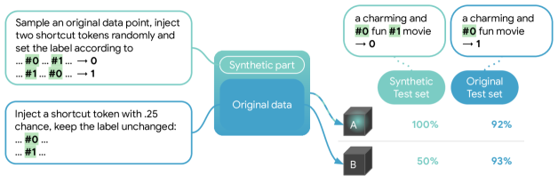
Figure 3: Illustration of how the ordered-pair shortcut is introduced into a balanced binary sentiment dataset and how it is verified that the shortcut is learned by the model. The model trained on the mixed data (A) is still largely a black box, but since its performance on the synthetic test set is 100% (contrasted with chance accuracy of model B which is similar but is trained on the original data only), we know it uses the injected shortcut (highlighted text).

2.2 Shortcut Types

A shortcut can be defined as a decision rule that a model learned from its training dataset which is not expected to hold under a slight distribution shift. While it is not possible to adequately characterize the full spectrum of thinkable shortcuts, one can identify common shortcut types which one anticipates to be learnable from a dataset. In this study we focus on lexical shortcuts that are characteristic of what modern classification models learn from text data. The following reasons motivate our choice. (i) Salience explanations are weights over tokens, hence lexical shortcuts (unlike more abstract ones, like overlap or syntactic cues) are a natural choice for them. Indeed, how easy would it be for a human to spot even a simple grammatical-positional rule (e.g., a coordinated NP at a certain position in the input) from a dozen highlights? Furthermore, it has been pointed out that input salience methods, unlike data attribution ones, may be insufficient for discovering artifacts beyond the lexical level Han et al. (2020). (ii) As mentioned in Introduction, lexical shortcuts represent a prominent failure mode for NLP models, therefore focusing on those we address probably the most important class of problems that salience methods could be helpful with. That being said, the proposed methodology can be easily extended to other shortcut types, as long as it makes sense to visualize the shortcut with a highlight over the input.

We consider three variants of lexical shortcuts:

Single token (st):

The simplest possible and still realistic shortcut (recall the NLI negation and toxicity identity examples) is a single token heuristic where the presence of a token determines the classification label. E.g., #0 and #1 indicate whether the label is 0 or 1.

Token in context (tic):

Another realistic lexical shortcut, which may be considerably more difficult to spot by a human but is still trivial to learn for a deep model, makes use of more than a single token. For example, two tokens determine the label together but not separately. We implement a token-in-context shortcut where the class indicator tokens (#0 or #1) only determine the label if yet another special token is present in the same input (contoken) but not on their own.

Ordered pair (op):

Yet another property of natural languages that a model can easily make use of is the order: a combination of tokens is predictive of the label only if the tokens occur in a certain order but not otherwise. We implement an ordered pair shortcut in its simplest form. That is, for an indicator token pair, (#0, #1), the order of the tokens determines the label so that ‘ … #0… #1…’ has label 0 and ‘ … #1… #0…’ has label 1. In other words, the first indicator token "gives away" the label. Again, neither of the indicator tokens, #0 and #1, is predictive of the label if occurring individually.

Why are contextuality and order worth modeling? Consider the IMDB review example from Ross et al. (2021) where BERT models learn to rely on numeric ratings present in the input. The learned shortcuts are multi-token – ‘3’ alone is by no means an indicator of a negative review. The order and proximity are important too: ‘3’, ‘out’, ‘of’ and ‘10’ mentioned far apart or in a different order are not predictive of the negative class. Thus, while other shortcut properties could be proposed, we do believe that the phenomena we model here for lexical shortcuts – namely, context and order – are representative of the poor generalization patterns of NLP models.

2.3 Creating (Partially) Synthetic Data

To ensure that the shortcut deterministically indicates the right label, we define shortcuts over tokens absent from the original dataset and introduce them explicitly in the vocabulary. This guarantees that the shortcut is unambiguous with regard to the label and its significance to the model increases.

Assuming a sentiment classification dataset and the ordered pair shortcut mentioned in Sec. 2.2 (the procedure is analogous for other data-shortcut combinations), we create a synthetic example by (1) randomly sampling an instance from the source data, (2) randomly deciding on the order of the shortcut tokens, (3) inserting these tokens at random positions, obeying the order and (4) setting the label as the shortcut prescribes. This process is illustrated in Fig. 3 (top left side). In all our experiments the resulting modified datasets are 20% larger than the source versions. The proportion of the synthetic data was not tuned but picked so that the shortcut data is sufficiently large to be picked by the model but not too large to deteriorate the performance on the unmodified data.

To mitigate the potential problem of making synthetic examples go off-manifold and thus being treated differently by the model as compared with the unmodified examples, for tic and so, we also inject one of the two tokens from the rule at random into a part of the original data without modifying the label. Thus, for multi-token shortcuts a special token can occur both in examples where it is predictive of the class as well as where it is not (bottom left of Fig. 3).

2.4 Verification Steps

The datasets we create are intentionally mixed and consist of the real and synthetic data to approximate real use cases where the model has to extract both simple and complex patterns to perform well. This is different from fully synthetic datasets Yang et al. (2018); Arras et al. (2019) or glass-box DNN models Hao (2020) where it is guaranteed that the model uses certain input features but the findings may not be valid for real datasets. Two tests verify that the model indeed uses the shortcut tokens and that they must be most important to the model:

1. The model should achieve close to 100% accuracy on the fully synthetic test set. This would imply that it learned the shortcut and consistently applies it on unseen data (hence the "transparent corner" of the top black box in Fig. 3).

2. The model trained on the original data (the bottom black box in Fig. 3) should perform at chance level on the same fully synthetic test set. This would imply that it is indeed the shortcut data and the shortcut rules that are needed to achieve 100% accuracy. In other words, no other tokens but the shortcut are useful to predict the label in that data.

3 Experimental Setup

We use three text classification datasets and apply the three shortcuts presented above to each of them. Despite all the datasets being binary and of comparable size, there are a few differences which may affect a salience method’s performance:

• SST2 Socher et al. (2013) is a balanced sentiment classification dataset with short (20 tokens on average) inputs;

• IMDB Maas et al. (2011) is also a balanced sentiment classification dataset with inputs about ten times longer than in SST2;

• Toxicity Wulczyn et al. (2017) is a varied length dataset containing toxicity annotations on Wikipedia comments where 9% of examples are positive (i.e., toxic). Aside from being imbalanced, it differs from the other two in that a text is toxic if it contains a single toxic phrase while for a movie review it is the dominating sentiment which determines the label.

In the results section we use the following format to refer to a dataset-shortcut combination: SST2:tic, IMDB:op, Toxicity:st, etc.

3.1 Models

We apply the salience methods to explain the predictions of two popular models: a bi-LSTM model Schuster et al. (1997) which uses GloVe embeddings Pennington et al. (2014), and BERT Devlin et al. (2019). Since we only consider binary tasks, the predicted probability of class $c\in\{0,1\}$ is given by the sigmoid function:

$$p(c|\mathbf{x}_{1:n})=\sigma(f_{c}(\mathbf{x}_{1:n}))$$ (3)

where $f_{c}(\cdot)$ denotes the model output for class $c$ and $\mathbf{x}_{1:n}$ is an input of $n$ token embeddings. Both models embed input tokens with a trainable layer so that every $\mathbf{x}_{i}$ is a continuous $d$-dimensional embedding vector of the $i$-th input token.

The models’ accuracy on all the source datasets are presented in Table 1. To verify that the models rely on the introduced shortcuts (Sec. 2.4), we computed the minimum and mean accuracy on all the nine fully synthetic test sets: these are 99.8 and 99.95 for LSTM and 99.7 and 99.91 for BERT (100% in most cases). The models trained on the original data (Table 1) all got 50% accuracy on the same synthetic test sets. The close to 100% performance on the synthetic data did not come at the cost of poor performance on the source test data: Table 1 reports the mean drop in accuracy averaged over the three shortcut models for each of the dataset and architecture combination.

	SST2	IMDB	Toxicity
LSTM	87.8 (0.6)	91.9 (0.0)	92.5 (0.0)
BERT	93.1 (0.6)	93.5 (0.2)	93.2 (0.2)

Table 1: Accuracy on the three source (unmodified) test sets of the models trained on the source training data. In brackets we report the mean drop in accuracy (on the same source test sets) when evaluating the models trained on a shortcut version of the training data.

3.2 Salience Methods

We consider four classes of input salience methods and the Random baseline (rand) to obtain per-token importance weights: Gradient (grad*), Gradient times Input (gxi*), Integrated Gradients (ig*) and lime.

3.2.1 Gradient

Li et al. (2016) use gradients as salience weights and compute a score per embedding dimension:

$$\nabla_{\mathbf{x}_{i}}f_{c}(\mathbf{x}_{1:n})$$ (4)

To arrive at the per-token score $s(\mathbf{x}_{i})$, Li et al. (2016) take the mean absolute value or the $L_{1}$ norm of the above vector’s components. Poerner et al. (2018) and Arras et al. (2019) use the $L_{2}$ norm, while Pezeshkpour et al. (2021) use the mean, referencing Atanasova et al. (2020).

Note that instead of $f_{c}$ one can compute the gradient of the final layer, that is, in our case the sigmoid function. An argument for starting from the probabilities is that, unlike logits, probabilities contain the information on the relative importance for a particular class. To our knowledge, the effect of using probabilities or logits has not been measured yet. In sum, we have six variants of the grad method: grad_{{p|l}×{l1|l2|mean}}.

3.2.2 Gradient times Input

Alternatively, one can compute salience weights by taking the dot product of Eq. 4 with the input word embedding $\mathbf{x}_{i}$ Denil et al. (2015) and obtain a salience weight for token $i$:

$$s(\mathbf{x}_{i})=\nabla_{\mathbf{x}_{i}}f_{c}(\mathbf{x}_{1:n})\cdot\mathbf{x}_{i}$$ (5)

Also here we can compare the probability and the logit versions: gxi_{p|l}.

3.2.3 Integrated Gradients

Integrated gradients (IG) (Sundararajan et al., 2017a) is a gradient-based method which addresses the problem of saturation: gradients may get close to zero for a well-fitted function. IG requires a baseline $\mathbf{b}_{1:n}$ as a way of contrasting the given input with information being absent. A zero vector Mudrakarta et al. (2018), the average embedding or unk or [mask] vectors can serve as baseline vectors in NLP. For input $i$, we compute:

$$\frac{1}{m}\!\!\sum_{k=1}^{m}\!\!\nabla_{\mathbf{x}_{i}}f_{c}\!\Big{(}\!\mathbf{b}_{1:n}\!\!+\!\frac{k}{m}\!(\mathbf{x}_{1:n}\!-\!\mathbf{b}_{1:n})\!\Big{)}\!\cdot\!(\mathbf{x}_{i}\!-\!\mathbf{b}_{i})\!$$ (6)

That is, we average over $m$ gradients, with the inputs to $f_{c}$ being linearly interpolated between the baseline and the original input $\mathbf{x}_{1:n}$ in $m$ steps. We then take the dot product of that averaged gradient with the input embedding $\mathbf{x}_{i}$ minus the baseline.

In addition to the variable number of steps–small (100) or large (1000)–and the baseline (zero vector, model-specific unk / [mask] or pad / [pad]), also here we can start either from probabilities (i.e., $\sigma$) or logits (i.e., $f$) and arrive at eight different IG configurations: ig_{{p|l}×{zero|mask}×{100|1000}}.

3.2.4 LIME

Ribeiro et al. (2016) train a linear model to estimate salience of input tokens on a number of perturbations, which are all generated from the given example $\mathbf{x}_{1:n}$. A perturbation is an instance where a random subset of tokens in $\mathbf{x}$ is masked out using either unk (LSTM, BERT) or [mask] (BERT) tokens, or dropped completely: erase (LSTM, BERT). The text model’s prediction on these perturbations is the target for the linear model, the masks are the inputs. Following Ribeiro et al. (2016) we use an exponential kernel with cosine distance and kernel width of 25 as proximity measure of instance and perturbations. We keep beginning and end-of-sequence tokens unperturbed and experiment with the number of perturbations (100, 1000, 3000). This results in 6 and 9 configurations for LSTM and BERT, respectively: lime_{{unk|mask|erase}×{100|1000|3000}}.

	SST2 P			IMDB P			Toxicity P
	st	tic	op	st	tic	op	st	tic	op
LSTM gxi{p|l}	1.	.76	.92	1.	.35	.81	1.	.68	.88
BERT gxi{p|l}	.29	.58	.31	.59	.35	.50	.41	.43	.47

Table 2: Precision gxi results across different models and datasets. Here and in the following tables P stands for Precision. Colors and boldface mark the results that are mentioned in the Results section. st: single token, tic: token in context, op: ordered pair. Here we see that performance of gxi varies across LSTM and BERT, i.e. the LSTM has consistently higher scores on all metrics (in bold). Perfect precision on the single-token shortcut doesn’t generalize to strong performance on two-token shortcuts (e.g., SST2:tic or IMDB:tic, ).

		SST2 P			IMDB P			Toxicity P			Toxicity R
		st	tic	op	st	tic	op	st	tic	op	st	tic	op
LSTM	grad{p|l}×l1	.96	.50	.51	1.	.50	.52	.29	.53	.55	2	26	13
	grad{p|l}×l2	.95	.50	.51	1.	.50	.52	.37	.54		2	26	13
	grad{p|l}-mean	.28	.23	.28	.25	.27	.20	.59	.48	.60	6	31	21
BERT	grad{p|l}×{l1|l2}	.99	.99	1.	.99	.87	.96	.99	.99	1.	1	2	2
	gradl-mean	.41	.44	.42	.41	.38	.41	.41	.45	.44	48	70	72
	gradp-mean	.43	.45	.42	.39	.34	.41	.44	.46	.44	43	74	72

Table 3: grad Precision across different models and datasets and grad Rank on the Toxcity dataset across models. Here and in the following tables R stands for Rank. grad_l2 performs very well for BERT (in bold) but not at all so for the LSTM model. The results of grad_mean are very poor, ranging between .34 and .46 in precision ( ). Rank and precision give complementary information: the precision of grad_l2 and grad_mean is close on Toxicity:op (.56 and .60) while the rank of the latter is almost twice as big (13 and 21) ( ).

4 Results

In this section we highlight our main findings. For increased readability where Rank scores support Precision, we omit them in the main paper and instead present them in the Appendix A.4. All the results reported in the paper are computed from a single model checkpoint and a single run.

A method’s performance varies across model and shortcut types and other dataset properties.

It is apparent that gxi performs quite well for LSTM models but does not work at all for BERT models (Tab. 2). Conversely, grad_l2 performs very well for BERT but not at all so for LSTM models (Tab. 3). Overall, method performance mostly goes down on longer inputs. More interestingly, a strong performance on a simpler shortcut may not persist on a slightly more complex one: gxi has precision of 1.0 on any dataset with the single-token shortcut for LSTM but drops to .76 or even .35 on the same base dataset with a two-token shortcut (e.g., SST2:tic or IMDB:tic, in Tab. 2). Thus, even if the model is fixed it cannot be assumed that a certain method works well and would be useful for finding lexical shortcuts learned by the model in general if its evaluation was done on only the single-token shortcut.

grad_{l|p}×l∗ is a good choice for BERT but not LSTM models for finding shortcuts.

For BERT models, grad_l2 achieves high precision and rank scores across the different datasets and shortcut types, yielding 0.99 or higher on seven out of nine datasets (Tab. 3 and 7). The lowest but still comparatively high precision (0.87) is on IMDB:tic where the inputs are particularly long. For LSTM models, on six out of nine datasets the precision of the same method is around .5 ( in Tab. 3). It does not matter whether probabilities or logits are used and whether L1 or L2 norm is applied. We hypothesize that one reason for the difference in performance between BERT and LSTM is that BERT models have residual connections, making the gradient information less noisy. However, the results of grad_mean are very poor, ranging between .3 and .4 in precision ( in Tab. 3). Note that grad_l2 is sometimes deemed unsuitable because it is unsigned and only returns positive scores Pezeshkpour et al. (2021), but our experiments demonstrate that it is the most useful method for finding lexical shortcuts learned by BERT.

Using probabilities instead of logits only changes the results for ig.

For other gradient-based methods it does not seem to make a large difference. ( and in Tab. 4 and 8).

ig performance does not improve much with more steps.

Increasing the number of interpolation steps from 100 to 1000 does not result in a significant improvement for LSTM models. Also for BERT, the precision numbers improve only for the tic shortcuts and only when probabilities are used (last two rows in Tab. 4 and 8). The similarity of the scores between the gxi and ig when using the zero baseline ( in Tab. 4 and 8) indicates that there is no difference between taking a single or 100(0) steps from the zero baseline.

		SST2 P			IMDB P			Toxicity P
		st	tic	op	st	tic	op	st	tic	op
LSTM	igl-zero-{100|1000}	1.	.72	.83	.99	.67	.80	1.	.95	.95
	igl-unk-{100|1000}	1.	.87	.71	1.	.71	.79	1.	.71	.78
	igl-pad-{100|1000}	1.	.77	.85	.99	.67	.79	1	.68	.67
	igp-zero-{100|1000}	.93	.69	.68	.78	.66	.76	1.	.93	.87
	igp-unk-{100|1000}	1.	.82	.77	1.	.70	.63	1.	.64	.63
	igp-pad-{100|1000}	.95	.74	.78	.83	.67	.75
BERT	gxi{p|l}	.29	.58	.31	.59	.35	.50	.41	.43	.47
	igl-zero-{100|1000}	.29	.58	.31	.59	.35	.50	.41	.43	.47
	igl-mask-{100|1000}	.71	.58	.71	.99	.62	.61	.69	.50	.47
	igl-pad-{100|1000}	.79	.27	.14	.28	.47	.27	.36	.46	.18
	igp-zero-{100|1000}	.29	.58	.31	.59	.35	.50	.41	.43	.47
	igp-mask-100
	igp-mask-1000	.48	.48	.56	.80	.47	.48	.28	.29	.29
	igp-pad-{100|1000}	.81	.18	.1	.21	.31	.14	.16	.37	.12

Table 4: IG Precision across different models and datasets. Using probabilities instead of logits changes the results for ig ( and ). Number of steps doesn’t affect the ig performance, but the choice of the baseline is important for ig when using BERT ( ). Using the [mask] baseline (with logits) resulted in an improvement in the scores (bold). Finally, rows tell us that the difference between gxi and ig_{p-zero-{100|1000}} is minimal and there is no difference between taking a single or 100(0) steps from the zero baseline.

		SST2 P			IMDB P			Toxicity P
		st	tic	op	st	tic	op	st	tic	op
LSTM	limeunk-100	.98	.80	.83	.92	.50	.62	.93	.58	.59
	limeunk-1000	1.	.83	.85	.99	.66	.78	1.	.84	.66
	limeunk-3000	1.	.84	.85	1.	.66	.80	1.	.85	.66
BERT	limeunk-100	.89	.80	.71	.91	.62	.44	.67	.54	.51
	limeunk-1000	.97	.87	.77	.99	.75	.70	.98	.58	.75
	limeunk-3000	.98	.88	.77	.99	.77	.71	1.	.59	.78
	limemask-3000	.98	.62	.78	.93	.76	.67	.99	.58	.70

Table 5: LIME Precision across different models and datasets. LIME benefits from 1000 over 100 perturbations, especially for longer inputs and/or shortcuts. We found that the increase from 1000 to 3000 perturbations leads to little precision improvements for the input lengths in our datasets. Using unk for masking leads to better results than [mask] in several configurations ( ).

Choice of baseline is important for ig when using BERT.

For the most part using the [mask] baseline (with logits) resulted in an improvement in the scores (bold rows in Tab. 4 and  8). Still, even with the best performing configuration of ig the results are much worse than grad_l-l2.

Number of perturbations as well as masking token matter for lime.

LIME benefits from 1000 over 100 perturbations, especially for longer inputs and/or shortcuts. We found that the increase from 1000 to 3000 perturbations leads to little precision improvements for the input lengths in our datasets. Using unk for masking leads to better results than [mask] in almost all configurations ( in Tab. 5 and 9). We hypothesize this is due to two reasons: (i) The [mask] token is not used during fine-tuning on the task data. (ii) The unk token, however, is finetuned (due to unknown tokens and as special token in word dropout). Erasing tokens leads, on average, to worse precision results than masking, for all number of perturbations. Tables 10 and 11 in Appendix A.5 present the results for all the models, shortcut types and source datasets in terms of precision and rank and you can observe this phenomenon there.

Rank and precision give complementary information.

For example, the precision of grad_l2 and grad_mean is close on Toxicity:op (.56 and .60) while the rank of the latter is almost twice as big (13 and 21) ( in Tab. 3). Lower rank with comparable precision means that the method consistently puts one of the shortcut tokens on the top but buries the other token deep in the ranking.

5 Related Work

Research on input salience methods for text classification is prolific and diverse in terms of the definitions used Camburu et al. (2020), applications Feng and Boyd-Graber (2019), desiderata Sundararajan et al. (2017b), etc. The importance of getting faithful salience explanations has been recognized early on Bach et al. (2015); Kindermans et al. (2017) and there exist formal definitions of explanation fidelity Yeh et al. (2019). However, these have not been connected to model debugging where it is the top of a salience ranking that matters most. In the vision domain, our work is closest to Adebayo et al. (2020, 2022), who also explore the debugging scenario with salience maps, Yang and Kim (2019), who use synthetic data to obtain the ground truth for pixel importance, and Hooker et al. (2019), who contrast the performance of the same model trained on original and modified data when evaluating feature importance.

As pointed out in Introduction, in NLP faithfulness evaluation has often been grounded in strong assumptions Poerner et al. (2018); DeYoung et al. (2020); Atanasova et al. (2020); Ding and Koehn (2021) or by analyzing models substantially different from the ones normally used Arras et al. (2019); Hao (2020). An exception to this trend is the work by Sippy et al. (2020) who also modify source data but, unlike us, consider MLP as the only DNN model, do not evaluate any gradient-based methods and analyze single token shortcuts only without strong guarantees of them actually being the most important clues for the model. Also Zhou et al. (2021) analyze DNN models on intentionally corrupted data: they primarily focus on vision but also run an experiment analyzing how faithfully the attention mechanism points at the words known to correlate with the label. Finally, Madsen et al. (2021), following Hooker et al. (2018), iteratively remove tokens to evaluate faithfulness of salience methods for LSTM models and conclude, similar to us, that performance is task-dependent.

Concurrently with our work, Idahl et al. (2021) argue for faithfulness evaluation on synthetic data for model debugging but do not report experimental results. Similarly to them and also concurrently with our work, Pezeshkpour et al. (2021) go further and combine data and input attribution methods to discover data artifacts. However, citing prior work, they use grad_l-mean and ig_l-mean which, as we have shown, are sub-optimal configurations for BERT models. This explains the very poor accuracy of 12-13% (in our terms: precision@1) that they observed when discovering single-token shortcuts in SST2. Finally, as our experiments demonstrate, the single-token shortcut is insufficient to assess whether a method would be useful for more complex shortcuts.

6 Conclusions

We have argued for evaluating input salience methods with respect to how helpful they would be for discovering shortcuts that are learned by the model. This seems to be a clear use case from the model developer perspective. To achieve this, we proposed a protocol for method evaluation and applied it to three variants of lexical shortcuts (single token, token in context, and ordered pair) which are a proxy for shortcut heuristics that occur in common NLP tasks and which are particularly suitable for being discovered with input salience methods. By comparing the performance across different datasets, shortcut types and models (LSTM-based and BERT-based), we demonstrated that a strong performance for one setup may not hold for a different model or a more complex shortcut. Finally, we pointed out that some method configurations assumed to be reliable in recent work, for example integrated gradients, may give very poor results for NLP models, and that the details of how the methods are used can matter a lot, such as how a gradient vector is reduced into a scalar. Our results demonstrate that whenever one uses BERT and is interested if a simple token combination could determine the label, one should prefer Grad-L2 over more complex methods.

7 Limitations

In this paper we proposed a protocol that can be used for evaluating input salience methods. We limited ourselves to the most popular salience methods, and left others out of scope. In particular, it would be of interest to evaluate the most recent salience methods, like Chen et al. (2020); Sikdar et al. (2021), which were developed to take feature interactions into account. We also limited this work to the task of English (binary) text classification. Furthermore, we focus on a representative set of shortcuts, but different shortcuts might result in different outcomes. Finally, we limited ourselves to LSTM and BERT based models. Results with different neural components or with models of a different size and/or depth may be different. However, the protocol that we proposed can still be used in those cases. We also note that input salience is only one kind of explanation, and a limited one: it does not reveal the logic of the model, nor does it reveal interactions between input features. It is hardly possible to fully understand why a deep non-linear neural model produced a certain prediction by only looking at input salience scores.

Acknowledgements

We would like to thank Ian Tenney, Alon Jacovi and the anonymous reviewers for the many helpful suggestions.

Appendix A Appendix

A.1 Architecture and training details

LSTM

For all datasets we use the same LSTM model consisting of an embedding layer that is initialized with a pretrained GloVe embedding, a single bidirectional LSTM layer and an attention classifier layer. The attention classifier consists of a keys-only attention layer Bahdanau et al. (2014); Jain and Wallace (2019) followed by a single layer MLP. The embedding size is $300$ and the word dropout rate is $0.1$, the LSTM and the classifier hidden sizes are set to $256$. The output size of the classifier is set to $1$. During training we use the same dropout rate of $0.5$ in all layers. We train this model with an SGD optimizer with a learning rate of $0.03$, momentum $0.9$ and a weight decay of $5\mathrm{e}{-6}$. We trained our models at most for $35000$ steps, however we enabled early stopping if after $10000$ steps we didn’t observe scores improvement on the validation set. For SST2 and IMDB we used a batch size of $64$ and for the Toxicity we used the size of $32$. With these hyper-parameters the LSTM models contain $5468048$ (5.4M) parameters.

BERT

For all datasets we use BERT Base model: 12 layers, 12 heads and a hidden size of 768. We load the publicly available pretrained uncased checkpoint before finetuning on our data. During training we use the same dropout rate of $0.5$. We chose the ADAM optimizer, with a learning rate of $2\mathrm{e}{-5}$ and a weight decay of $5\mathrm{e}{-6}$ following the best practices of finetuning BERT Devlin et al. (2019). For Toxicity we set the learning rate to $1\mathrm{e}{-5}$, the rest of the parameters are the same. The maximum sequence length in SST2 we set to 100, and for IMDB and Toxicity we set it to 500. We follow the same early stopping configuration as in LSTM. We use a batch size of 16 everywhere. With these hyper-parameters the BERT (Base) models contain $109483009$ (109M) parameters.

A.2 Budget

For our experiments we used a total of 35 hours on TPUv2 (4-core) accelerators.

A.3 Methods implementation details

Integrated gradients

For the non-zero IG baseline, we take the sequence of embedded inputs, keep the embeddings of the special tokens (e.g. CLS and SEP) the same, and replace the other embedded inputs with the embedded baseline token (e.g., MASK or UNK).

A.4 Rank results

Please refer to Tables 6, 8, 7, 9 for the Rank results that complete the story in the paper.

	SST2			IMDB			Toxicity
	st	tic	op	st	tic	op	st	tic	op
LSTM	1	8	3	1	212	24	1	16	5
BERT	17	17	24	106	214	189	33	88	69

Table 6: gxi Rank results across different models and datasets. Here we see that performance of gxi varies across LSTM and BERT, i.e. LSTM has consistently higher scores on all metrics (in bold).

	SST2 R			IMDB R			Toxicity R
	st	tic	op	st	tic	op	st	tic	op
LSTM	1	11	15	1	22	51	2	26	13
	1	11	15	1	22	50	2	26	13
	7	21	20	152	123	153	6	31	21
BERT	1	2	2	1	2	2	1	2	2
	12	21	21	132	203	206	48	70	72
	13	21	21	134	204	204	43	74	72

Table 7: grad Rank across different models and datasets.

		SST2 R			IMDB R			Toxicity R
		st	tic	op	st	tic	op	st	tic	op
LSTM	igl-zero-{100|1000}	1	11	6	1	118	97	1	3	3
	igl-unk-{100|1000}	1	6	12	1	112	94	1	29	20
	igl-pad-{100|1000}	1	10	6	1	126	100	1	26	20
	igp-zero-{100|1000}	1	11	8	3	118	97	1	3	9
	igp-unk-{100|1000}	1	8	10	1	117	117	1	39	36
	igp-pad-{100|1000}	1	10	7	2	126	105	1	44	32
BERT	gxi{p|l}	17	17	24	106	214	189	33	88	69
	igl-zero-{100|1000}	16	17	24	105	213	190	33	88	69
	igl-mask-{100|1000}	2	13	6	1	110	82	4	63	40
	igl-pad-{100|1000}	4	18	14	120	243	141	3	92	31
	igp-zero-{100|1000}	16	17	24	105	213	190	33	88	69
	igp-mask-100
	igp-mask-1000	5	13	9	10	106	95	31	66	50
	igp-pad-{100|1000}	3	18	15	114	219	153	11	83	47

Table 8: IG Rank across different models and datasets. Similarly to the precision results from Tab. 4 we see that using probabilities instead of logits changes the results for ig ( ). We also observe that number of steps doesn’t affect the ig performance, but the choice of baseline is important for ig when using BERT ( ). Finally rows tell us the difference between gxi and ig_{p-zero-{100|1000}} is minimal and there is no difference between taking a single or 100(0) steps from the zero baseline.

		SST2 R			IMDB R			Toxicity R
		st	tic	op	st	tic	op	st	tic	op
LSTM	limeunk-100	1	7	4	2	99	67	1	13	34
	limeunk-1000	1	6	4	1	83	45	1	7	34
	limeunk-3000	1	6	4	1	82	40	1	8	33
BERT	limeunk-100	1	8	7	3	94	67	6	82	28
	limeunk-1000	1	7	6	2	96	57	1	78	23
	limeunk-3000	1	7	5	2	97	56	1	77	21
	limemask-3000	1	13	5	13	105	52	1	80	12

Table 9: LIME Rank across different models and datasets. Similarly to the precision results from Tab. 5 we see that LIME benefits from 1000 over 100 perturbations, especially for longer inputs and/or shortcuts. We found that the increase from 1000 to 3000 perturbations leads to little precision improvements for the input lengths in our datasets. Using unk for masking leads to better results than [mask] in almost all configurations ( ).

A.5 Full Results

Table 10 and Table 11 list the full results for LSTM and BERT respectively.

	SST2			IMDB			Toxicity			SST2			IMDB			Toxicity
	Precision			Precision			Precision			Rank			Rank			Rank
	st	tic	op	st	tic	op	st	tic	op	st	tic	op	st	tic	op	st	tic	op
random	.06	.1	.1	.0	.01	.01	.03	.07	.06	11	16	17	120	161	162	27	36	36
grad{p|l}×l1	.96	.5	.51	1.	.5	.52	.29	.53	.55	1	11	15	1	22	51	2	26	13
grad{p|l}×l2	.95	.5	.51	1.	.5	.52	.37	.54	.56	1	11	15	1	22	50	2	26	13
grad{p|l}-mean	.28	.23	.28	.25	.27	.2	.59	.48	.6	7	21	20	152	123	153	6	31	21
gxi{p|l}	1.	.76	.92	1.	.35	.81	1.	.68	.88	1	8	3	1	212	24	1	16	5
igl-zero-100	1	.72	.83	.99	.67	.80	1	.95	.95	1	11	6	1	118	97	1	3	3
igl-zero-1000	1	.72	.83	1	.67	.79	1	.95	.95	1	11	6	1	118	95	1	3	3
igl-unk-100	1	.87	.71	1	.71	.79	1	.71	.78	1	6	12	1	112	94	1	29	20
igl-unk-1000	1	.88	.71	1	.71	.81	1	.71	.78	1	6	12	1	113	89	1	30	20
igp-zero-100	.93	.69	.68	.78	.66	.76	1	.93	.87	1	11	8	3	118	97	1	3	9
igp-zero-1000	.93	.69	.68	.75	.66	.77	1	.93	.87	1	11	8	3	118	95	1	3	9
igp-unk-100	1	.82	.77	1	.70	.63	1	.64	.63	1	8	10	1	117	117	1	39	36
igp-unk-1000	1	.82	.77	1	.70	.65	1	.64	.62	1	8	10	1	117	111	1	40	37
limeunk-100	.98	.80	.83	.92	.50	.62	.93	.58	.59	1	7	4	2	99	67	1	13	34
limeunk-1000	1.	.83	.85	.99	.66	.78	1.	.84	.66	1	6	4	1	83	45	1	7	34
limeunk-3000	1.	.84	.85	1.	.66	.80	1.	.85	.66	1	6	4	1	82	40	1	8	33
limeerase-100	.93	.68	.74	.77	.50	.60	.97	.69	.44	1	8	9	7	120	75	1	9	32
limeerase-1000	.99	.72	.77	.97	.72	.76	1.	.94	.68	1	7	8	1	83	55	1	2	33
limeerase-3000	1.	.72	.77	.99	.73	.77	1.	.96	.70	1	7	8	1	76	50	1	2	33

Table 10: Precision and rank of all the method configurations across the datasets and shortcut types for LSTM. st: single token, tic: token in context, op: ordered pair.

	SST2			IMDB			Toxicity			SST2			IMDB			Toxicity
	Precision			Precision			Precision			Rank			Rank			Rank
	st	tic	op	st	tic	op	st	tic	op	st	tic	op	st	tic	op	st	tic	op
grad{p|l}×{l1|l2}	.99	.99	1.	.99	.87	.96	.99	.99	1.	1	2	2	1	2	2	1	2	2
gradl-mean	.41	.44	.42	.41	.38	.41	.41	.45	.44	12	21	21	132	203	206	48	70	72
gradp-mean	.43	.45	.42	.39	.34	.41	.44	.46	.44	13	21	21	134	204	204	43	74	72
gxi{p|l}	.29	.58	.31	.59	.35	.50	.41	.43	.47	17	17	24	106	214	189	33	88	69
igl-zero-{100|1000}	.29	.58	.31	.59	.35	.50	.41	.43	.47	16	17	24	105	213	190	33	88	69
igl-mask-100	.71	.58	.71	.99	.62	.61	.69	.50	.47	2	13	6	1	110	82	4	63	40
igl-mask-1000	.71	.58	.71	.99	.64	.61	.70	.50	.47	2	14	5	1	109	83	4	65	41
igp-zero-{100|1000}	.29	.58	.31	.59	.35	.50	.41	.43	.47	16	17	24	105	213	190	33	88	69
igp-mask-100	.48	.37	.56	.80	.34	.48	.27	.27	.29	5	14	8	17	115	93	31	64	50
igp-mask-1000	.48	.48	.56	.80	.47	.48	.28	.29	.29	5	13	9	10	106	95	31	66	50
limeunk-100	.89	.80	.71	.91	.62	.44	.67	.54	.51	1	8	7	3	94	67	6	82	28
limeunk-1000	.97	.87	.77	.99	.75	.70	.98	.58	.75	1	7	6	2	96	57	1	78	23
limeunk-3000	.98	.88	.77	.99	.77	.71	1.	.59	.78	1	7	5	2	97	56	1	77	21
limemask-3000	.98	.62	.78	.93	.76	.67	.99	.58	.70	1	13	5	13	105	52	1	80	12
limeerase-100	.83	.61	.63	.96	.62	.53	.59	.54	.40	2	13	6	1	97	55	9	83	42
limeerase-1000	.93	.63	.65	1.	.77	.71	.88	.59	.55	1	13	4	1	95	32	3	78	31
limeerase-3000	.94	.63	.65	1.	.78	.74	.94	.59	.58	1	13	4	1	96	27	1	78	28

Table 11: Precision and rank of all the method configurations across the datasets and shortcut types for BERT.

References

- Adebayo et al. (2022) Julius Adebayo, Michael Muelly, Harold Abelson, and Been Kim. 2022. Post hoc explanations may be ineffective for detecting unknown spurious correlation. In International Conference on Learning Representations.
- Adebayo et al. (2020) Julius Adebayo, Michael Muelly, Ilaria Liccardi, and Been Kim. 2020. Debugging tests for model explanations. In NeurIPS.
- Arras et al. (2019) Leila Arras, Ahmed Osman, Klaus-Robert Müller, and Wojciech Samek. 2019. Evaluating recurrent neural network explanations. In Proceedings of the 2019 ACL Workshop BlackboxNLP: Analyzing and Interpreting Neural Networks for NLP, pages 113–126, Florence, Italy. Association for Computational Linguistics.
- Atanasova et al. (2020) Pepa Atanasova, Jakob Grue Simonsen, Christina Lioma, and Isabelle Augenstein. 2020. A diagnostic study of explainability techniques for text classification. In Proceedings of the 2020 Conference on Empirical Methods in Natural Language Processing (EMNLP), pages 3256–3274, Online. Association for Computational Linguistics.
- Bach et al. (2015) Sebastian Bach, A. Binder, G. Montavon, F. Klauschen, Klaus-Robert Müller, and W. Samek. 2015. On pixel-wise explanations for non-linear classifier decisions by layer-wise relevance propagation. PLoS ONE, 10(7).
- Bahdanau et al. (2014) Dzmitry Bahdanau, Kyunghyun Cho, and Yoshua Bengio. 2014. Neural machine translation by jointly learning to align and translate. arXiv preprint arXiv:1409.0473.
- Bastings and Filippova (2020) Jasmijn Bastings and Katja Filippova. 2020. The elephant in the interpretability room: Why use attention as explanation when we have saliency methods? In Proceedings of the Third BlackboxNLP Workshop on Analyzing and Interpreting Neural Networks for NLP, pages 149–155, Online. Association for Computational Linguistics.
- Belinkov et al. (2019) Yonatan Belinkov, Adam Poliak, Stuart Shieber, Benjamin Van Durme, and Alexander Rush. 2019. Don’t take the premise for granted: Mitigating artifacts in natural language inference. In Proceedings of the 57th Annual Meeting of the Association for Computational Linguistics, pages 877–891, Florence, Italy. Association for Computational Linguistics.
- Camburu et al. (2019) Oana-Maria Camburu, Eleonora Giunchiglia, Jakob Foerster, Thomas Lukasiewicz, and Phil Blunsom. 2019. Can I trust the explainer? verifying post-hoc explanatory methods. In NeurIPS 2019 Workshop on Safety and Robustness in Decision Making, Vancouver, Canada.
- Camburu et al. (2020) Oana-Maria Camburu, Eleonora Giunchiglia, Jakob Foerster, Thomas Lukasiewicz, and Phil Blunsom. 2020. The struggles of feature-based explanations: Shapley values vs. minimal sufficient subsets.
- Chen et al. (2020) Zhihong Chen, Yan Song, Tsung-Hui Chang, and Xiang Wan. 2020. Generating radiology reports via memory-driven transformer. In Proceedings of the 2020 Conference on Empirical Methods in Natural Language Processing (EMNLP), pages 1439–1449, Online. Association for Computational Linguistics.
- Codella et al. (2019) Noel Codella, Veronica Rotemberg, Philipp Tschandl, M. Emre Celebi, Stephen Dusza, David Gutman, Brian Helba, Aadi Kalloo, Konstantinos Liopyris, Michael Marchetti, Harald Kittler, and Allan Halpern. 2019. Skin lesion analysis toward melanoma detection 2018: A challenge hosted by the international skin imaging collaboration (isic).
- Denil et al. (2015) Misha Denil, Alban Demiraj, and Nando de Freitas. 2015. Extraction of salient sentences from labelled documents.
- Devlin et al. (2019) Jacob Devlin, Ming-Wei Chang, Kenton Lee, and Kristina Toutanova. 2019. BERT: Pre-training of deep bidirectional transformers for language understanding. In Proceedings of the 2019 Conference of the North American Chapter of the Association for Computational Linguistics: Human Language Technologies, Volume 1 (Long and Short Papers), pages 4171–4186, Minneapolis, Minnesota. Association for Computational Linguistics.
- DeYoung et al. (2020) Jay DeYoung, Sarthak Jain, Nazneen Fatema Rajani, Eric Lehman, Caiming Xiong, Richard Socher, and Byron C. Wallace. 2020. ERASER: A benchmark to evaluate rationalized NLP models. In Proceedings of the 58th Annual Meeting of the Association for Computational Linguistics, pages 4443–4458, Online. Association for Computational Linguistics.
- Ding and Koehn (2021) Shuoyang Ding and Philipp Koehn. 2021. Evaluating saliency methods for neural language models. In Proceedings of the 2021 Conference of the North American Chapter of the Association for Computational Linguistics: Human Language Technologies, pages 5034–5052, Online. Association for Computational Linguistics.
- Dixon et al. (2018) Lucas Dixon, John Li, Jeffrey Sorensen, Nithum Thain, and Lucy Vasserman. 2018. Measuring and mitigating unintended bias in text classification. In AAAI/ACM Conference on AI, Ethics, and Society.
- Du et al. (2021) Mengnan Du, Varun Manjunatha, Rajiv Jain, Ruchi Deshpande, Franck Dernoncourt, Jiuxiang Gu, Tong Sun, and Xia Hu. 2021. Towards interpreting and mitigating shortcut learning behavior of NLU models. In Proceedings of the 2021 Conference of the North American Chapter of the Association for Computational Linguistics: Human Language Technologies, pages 915–929, Online. Association for Computational Linguistics.
- Feng and Boyd-Graber (2019) Shi Feng and Jordan Boyd-Graber. 2019. What can ai do for me? evaluating machine learning interpretations in cooperative play. In Proceedings of the 24th International Conference on Intelligent User Interfaces, IUI ’19, page 229–239, New York, NY, USA. Association for Computing Machinery.
- Geirhos et al. (2020) R. Geirhos, J.-H. Jacobsen, C. Michaelis, R. Zemel, W. Brendel, M. Bethge, and F. A. Wichmann. 2020. Shortcut learning in deep neural networks. Nature Machine Intelligence, 2:665––673.
- Geva et al. (2019) Mor Geva, Yoav Goldberg, and Jonathan Berant. 2019. Are we modeling the task or the annotator? an investigation of annotator bias in natural language understanding datasets. In Proceedings of the 2019 Conference on Empirical Methods in Natural Language Processing and the 9th International Joint Conference on Natural Language Processing (EMNLP-IJCNLP), pages 1161–1166, Hong Kong, China. Association for Computational Linguistics.
- Gururangan et al. (2018) Suchin Gururangan, Swabha Swayamdipta, Omer Levy, Roy Schwartz, Samuel Bowman, and Noah A. Smith. 2018. Annotation artifacts in natural language inference data. In Proceedings of the 2018 Conference of the North American Chapter of the Association for Computational Linguistics: Human Language Technologies, Volume 2 (Short Papers), pages 107–112, New Orleans, Louisiana. Association for Computational Linguistics.
- Han et al. (2020) Xiaochuang Han, Byron C. Wallace, and Yulia Tsvetkov. 2020. Explaining black box predictions and unveiling data artifacts through influence functions. In Proceedings of the 58th Annual Meeting of the Association for Computational Linguistics, pages 5553–5563, Online. Association for Computational Linguistics.
- Hao (2020) Yiding Hao. 2020. Evaluating attribution methods using white-box LSTMs. In Proceedings of the Third BlackboxNLP Workshop on Analyzing and Interpreting Neural Networks for NLP, pages 300–313, Online. Association for Computational Linguistics.
- Hooker et al. (2018) Sara Hooker, Dumitru Erhan, Pieter jan Kindermans, and Been Kim. 2018. Evaluating feature importance estimates. arXiv.
- Hooker et al. (2019) Sara Hooker, Dumitru Erhan, Pieter-Jan Kindermans, and Been Kim. 2019. A benchmark for interpretability methods in deep neural networks. In Advances in Neural Information Processing Systems, volume 32, pages 9737–9748. Curran Associates, Inc.
- Idahl et al. (2021) Maximilian Idahl, Lijun Lyu, Ujwal Gadiraju, and Avishek Anand. 2021. Towards benchmarking the utility of explanations for model debugging. In Proceedings of the First Workshop on Trustworthy Natural Language Processing, pages 68–73, Online. Association for Computational Linguistics.
- Jacovi and Goldberg (2020) Alon Jacovi and Yoav Goldberg. 2020. Towards faithfully interpretable NLP systems: How should we define and evaluate faithfulness? In Proceedings of the 58th Annual Meeting of the Association for Computational Linguistics, pages 4198–4205, Online. Association for Computational Linguistics.
- Jain and Wallace (2019) Sarthak Jain and Byron C. Wallace. 2019. Attention is not Explanation. In Proceedings of the 2019 Conference of the North American Chapter of the Association for Computational Linguistics: Human Language Technologies, Volume 1 (Long and Short Papers), pages 3543–3556, Minneapolis, Minnesota. Association for Computational Linguistics.
- Kaushik et al. (2020) Divyansh Kaushik, Eduard H. Hovy, and Zachary Chase Lipton. 2020. Learning the difference that makes a difference with counterfactually-augmented data. In 8th International Conference on Learning Representations, ICLR 2020, Addis Ababa, Ethiopia, April 26-30, 2020. OpenReview.net.
- Kim et al. (2020) Siwon Kim, Jihun Yi, Eunji Kim, and Sungroh Yoon. 2020. Interpretation of NLP models through input marginalization. In Proceedings of the 2020 Conference on Empirical Methods in Natural Language Processing (EMNLP), pages 3154–3167, Online. Association for Computational Linguistics.
- Kindermans et al. (2017) Pieter-Jan Kindermans, Sara Hooker, Julius Adebayo, Maximilian Alber, Kristof T. Schütt, Sven Dähne, Dumitru Erhan, and Been Kim. 2017. The (un)reliability of saliency methods.
- Li et al. (2016) Jiwei Li, Xinlei Chen, Eduard Hovy, and Dan Jurafsky. 2016. Visualizing and understanding neural models in NLP. In Proceedings of the 2016 Conference of the North American Chapter of the Association for Computational Linguistics: Human Language Technologies, pages 681–691, San Diego, California. Association for Computational Linguistics.
- Maas et al. (2011) Andrew L. Maas, Raymond E. Daly, Peter T. Pham, Dan Huang, Andrew Y. Ng, and Christopher Potts. 2011. Learning word vectors for sentiment analysis. In Proceedings of the 49th Annual Meeting of the Association for Computational Linguistics: Human Language Technologies, pages 142–150, Portland, Oregon, USA. Association for Computational Linguistics.
- Madsen et al. (2021) Andreas Madsen, Nicholas Meade, Vaibhav Adlakha, and Siva Reddy. 2021. Evaluating the faithfulness of importance measures in nlp by recursively masking allegedly important tokens and retraining.
- McCoy et al. (2019) Tom McCoy, Ellie Pavlick, and Tal Linzen. 2019. Right for the wrong reasons: Diagnosing syntactic heuristics in natural language inference. In Proceedings of the 57th Annual Meeting of the Association for Computational Linguistics, pages 3428–3448, Florence, Italy. Association for Computational Linguistics.
- Mudrakarta et al. (2018) Pramod Kaushik Mudrakarta, Ankur Taly, Mukund Sundararajan, and Kedar Dhamdhere. 2018. Did the model understand the question? In Proceedings of the 56th Annual Meeting of the Association for Computational Linguistics (Volume 1: Long Papers), pages 1896–1906, Melbourne, Australia. Association for Computational Linguistics.
- Pavlopoulos et al. (2017) John Pavlopoulos, Prodromos Malakasiotis, and Ion Androutsopoulos. 2017. Deeper attention to abusive user content moderation. In Proceedings of the 2017 Conference on Empirical Methods in Natural Language Processing, pages 1125–1135, Copenhagen, Denmark. Association for Computational Linguistics.
- Pennington et al. (2014) Jeffrey Pennington, Richard Socher, and Christopher D. Manning. 2014. Glove: Global vectors for word representation. In Empirical Methods in Natural Language Processing (EMNLP), pages 1532–1543.
- Pezeshkpour et al. (2021) Pouya Pezeshkpour, Sarthak Jain, Sameer Singh, and Byron C. Wallace. 2021. Combining feature and instance attribution to detect artifacts.
- Poerner et al. (2018) Nina Poerner, Hinrich Schütze, and Benjamin Roth. 2018. Evaluating neural network explanation methods using hybrid documents and morphosyntactic agreement. In Proceedings of the 56th Annual Meeting of the Association for Computational Linguistics (Volume 1: Long Papers), pages 340–350, Melbourne, Australia. Association for Computational Linguistics.
- Poliak et al. (2018) Adam Poliak, Jason Naradowsky, Aparajita Haldar, Rachel Rudinger, and Benjamin Van Durme. 2018. Hypothesis only baselines in natural language inference. In Proceedings of the Seventh Joint Conference on Lexical and Computational Semantics, pages 180–191, New Orleans, Louisiana. Association for Computational Linguistics.
- Ribeiro et al. (2016) Marco Tulio Ribeiro, Sameer Singh, and Carlos Guestrin. 2016. "why should I trust you?": Explaining the predictions of any classifier. In Proceedings of the 22nd ACM SIGKDD International Conference on Knowledge Discovery and Data Mining, San Francisco, CA, USA, August 13-17, 2016, pages 1135–1144.
- Rosenman et al. (2020) Shachar Rosenman, Alon Jacovi, and Yoav Goldberg. 2020. Exposing Shallow Heuristics of Relation Extraction Models with Challenge Data. In Proceedings of the 2020 Conference on Empirical Methods in Natural Language Processing (EMNLP), pages 3702–3710, Online. Association for Computational Linguistics.
- Ross et al. (2021) Alexis Ross, Ana Marasović, and Matthew Peters. 2021. Explaining NLP models via minimal contrastive editing (MiCE). In Findings of the Association for Computational Linguistics: ACL-IJCNLP 2021, pages 3840–3852, Online. Association for Computational Linguistics.
- Samek and Müller (2019) Wojciech Samek and Klaus-Robert Müller. 2019. Towards Explainable Artificial Intelligence, pages 5–22. Springer International Publishing, Cham.
- Schmidt and Biessmann (2019) Philipp Schmidt and Felix Biessmann. 2019. Quantifying interpretability and trust in machine learning systems.
- Schuster et al. (1997) Mike Schuster, Kuldip K. Paliwal, and A. General. 1997. Bidirectional recurrent neural networks. IEEE Transactions on Signal Processing.
- Sikdar et al. (2021) Sandipan Sikdar, Parantapa Bhattacharya, and Kieran Heese. 2021. Integrated directional gradients: Feature interaction attribution for neural NLP models. In Proceedings of the 59th Annual Meeting of the Association for Computational Linguistics and the 11th International Joint Conference on Natural Language Processing (Volume 1: Long Papers), pages 865–878, Online. Association for Computational Linguistics.
- Sippy et al. (2020) Jacob Sippy, Gagan Bansal, and Daniel S. Weld. 2020. Data staining: A method for comparing faithfulness of explainers. In The Fifth Annual Workshop on Human Interpretability in Machine Learning (WHI 2020).
- Socher et al. (2013) Richard Socher, Alex Perelygin, Jean Wu, Jason Chuang, Christopher D. Manning, Andrew Ng, and Christopher Potts. 2013. Recursive deep models for semantic compositionality over a sentiment treebank. In Proceedings of the 2013 Conference on Empirical Methods in Natural Language Processing, pages 1631–1642, Seattle, Washington, USA. Association for Computational Linguistics.
- Strout et al. (2019) Julia Strout, Ye Zhang, and Raymond Mooney. 2019. Do human rationales improve machine explanations? In Proceedings of the 2019 ACL Workshop BlackboxNLP: Analyzing and Interpreting Neural Networks for NLP, pages 56–62, Florence, Italy. Association for Computational Linguistics.
- Sundararajan et al. (2019) M. Sundararajan, Jinhua Xu, Ankur Taly, R. Sayres, and A. Najmi. 2019. Exploring principled visualizations for deep network attributions. In IUI Workshops.
- Sundararajan et al. (2017a) Mukund Sundararajan, Ankur Taly, and Qiqi Yan. 2017a. Axiomatic attribution for deep networks. In Proceedings of the 34th International Conference on Machine Learning, ICML 2017, Sydney, NSW, Australia, 6-11 August 2017, volume 70 of Proceedings of Machine Learning Research, pages 3319–3328. PMLR.
- Sundararajan et al. (2017b) Mukund Sundararajan, Ankur Taly, and Qiqi Yan. 2017b. Axiomatic attribution for deep networks. In Proceedings of the 34th International Conference on Machine Learning, volume 70 of Proceedings of Machine Learning Research, pages 3319–3328, International Convention Centre, Sydney, Australia. PMLR.
- Tenney et al. (2020) Ian Tenney, James Wexler, Jasmijn Bastings, Tolga Bolukbasi, Andy Coenen, Sebastian Gehrmann, Ellen Jiang, Mahima Pushkarna, Carey Radebaugh, Emily Reif, and Ann Yuan. 2020. The language interpretability tool: Extensible, interactive visualizations and analysis for NLP models. In Proceedings of the 2020 Conference on Empirical Methods in Natural Language Processing: System Demonstrations, pages 107–118, Online. Association for Computational Linguistics.
- Winkler et al. (2019) Julia K. Winkler, Christine Fink, Ferdinand Toberer, Alexander Enk, Teresa Deinlein, Rainer Hofmann-Wellenhof, Luc Thomas, Aimilios Lallas, Andreas Blum, Wilhelm Stolz, and Holger A. Haenssle. 2019. Association Between Surgical Skin Markings in Dermoscopic Images and Diagnostic Performance of a Deep Learning Convolutional Neural Network for Melanoma Recognition. JAMA Dermatology, 155(10):1135–1141.
- Wulczyn et al. (2017) Ellery Wulczyn, Nithum Thain, and Lucas Dixon. 2017. Ex machina: Personal attacks seen at scale. In Proceedings of the 26th International Conference on World Wide Web, WWW ’17, pages 1391–1399, Republic and Canton of Geneva, CHE. International World Wide Web Conferences Steering Committee.
- Yang and Kim (2019) Mengjiao Yang and Been Kim. 2019. Benchmarking Attribution Methods with Relative Feature Importance. CoRR, abs/1907.09701.
- Yang et al. (2018) Yinchong Yang, Volker Tresp, Marius Wunderle, and Peter A. Fasching. 2018. Explaining therapy predictions with layer-wise relevance propagation in neural networks. In 2018 IEEE International Conference on Healthcare Informatics (ICHI), pages 152–162.
- Yeh et al. (2019) Chih-Kuan Yeh, Cheng-Yu Hsieh, Arun Suggala, David I Inouye, and Pradeep K Ravikumar. 2019. On the (in)fidelity and sensitivity of explanations. In Advances in Neural Information Processing Systems, volume 32. Curran Associates, Inc.
- Yin et al. (2022) Fan Yin, Zhouxing Shi, Cho-Jui Hsieh, and Kai-Wei Chang. 2022. On the sensitivity and stability of model interpretations in NLP. In Proceedings of the 60th Annual Meeting of the Association for Computational Linguistics (Volume 1: Long Papers), pages 2631–2647, Dublin, Ireland. Association for Computational Linguistics.
- Zhou et al. (2021) Yilun Zhou, Serena Booth, Marco Tílio Ribeiro, and Julie Shah. 2021. Do feature attribution methods correctly attribute features? CoRR, abs/2104.14403.