A Simple Algorithm for Multiple-Source Shortest Paths in Planar Digraphs

Abstract

Given an $n$-vertex planar embedded digraph $G$ with non-negative edge weights and a face $f$ of $G$, Klein presented a data structure with $O(n\log n)$ space and preprocessing time which can answer any query $(u,v)$ for the shortest path distance in $G$ from $u$ to $v$ or from $v$ to $u$ in $O(\log n)$ time, provided $u$ is on $f$. This data structure is a key tool in a number of state-of-the-art algorithms and data structures for planar graphs.

Klein’s data structure relies on dynamic trees and the persistence technique as well as a highly non-trivial interaction between primal shortest path trees and their duals. The construction of our data structure follows a completely different and in our opinion very simple divide-and-conquer approach that solely relies on Single-Source Shortest Path computations and contractions in the primal graph. Our space and preprocessing time bound is $O(n\log|f|)$ and query time is $O(\log|f|)$ which is an improvement over Klein’s data structure when $f$ has small size.

1 Introduction

In the Planar Multiple-Source Shortest Paths (MSSP) problem, an embedded digraph $G$ is given along with a distinguished face $f$, and the goal is to compute a data structure answering distance queries between any vertex pair $(u,v)$ where either $u$ or $v$ belong to $f$. Data structures for this problem are measured by the preprocessing time required to construct the data structure, the space required to store the data structure, and the query time required to answer a query.

Applications.

MSSP data structures are a crucial building block for the All-Pairs Shortest Paths (APSP) problem in planar graphs where the data structure needs to be able to return the (approximate or exact) distance between any two vertices in the graph. Such data structures are often called distance oracles if the query time is subpolynomial in $n$. Broadly, there are three different APSP data structure problems that currently rely on MSSP algorithms:

• Exact Distance Oracles: In a recent series of breakthroughs, [5, 14, 4, 20] showed that it is possible to obtain an APSP data structure that requires only space $n^{1+o(1)}$ and query time $n^{o(1)}$ where both [4] and the state-of-the-art result in [20] employs MSSP as a building block in their construction.

• Approximate Distance Oracles: Thorup [25] presented a data structure that returns $(1+\epsilon)$-approximate distance estimates using preprocessing time and space $\tilde{O}(n\epsilon^{-1})$ and query time $O(\log\log n+\epsilon^{-1})$. Since, his construction time was sped-up by polylogarithmic factors via improvements to the state-of-the-art MSSP data structure [18].

• Exact (Dynamic) APSP: A classic algorithm by Fakcharoenphol and Rao [11] gives a data structure that uses $\tilde{O}(n)$ space and preprocessing time, and takes query time $\tilde{O}(\sqrt{n})$ to answer queries exactly. A variant of this algorithm further gives a data structure that processes edge weight changes to the graph $G$ in time $\tilde{O}(n^{2/3})$ while still allowing for query time $\tilde{O}(n^{2/3})$. Again, while [11] did not directly employ an MSSP data structure, Klein [18] showed that incorporating MSSP leads to a speed-up in the logarithmic factors.

We point out that various improvements were made during the last years over these seminal results when considering different trade-offs [12, 21] or by improving logarithmic or doubly-logarithmic factors [23, 13, 22], however, the fundamental sub-problem of MSSP is present in almost all of these articles. We emphasize that beyond the run-time improvements achieved by MSSP data structure, an additional benefit is a more modular and re-usable design that makes it simpler to understand and implement APSP algorithms.

Another key application of MSSP is the computation of a dense distance graph. An often employed strategy for a planar graph problem is to decompose the embedded planar input graph $G$ into smaller graphs using vertex separators in order to either obtain a recursive decomposition or a flat so called $r$-division of $G$. For each subgraph $R$ obtained, let $\partial R$ denote its set of boundary vertices (vertices incident to edges not in $R$). The dense distance graph of $R$ is the complete graph on $\partial R$ where each edge $(u,v)$ is assigned a weight equal to the shortest path distance from $u$ to $v$ in $R$. Since the recursive or flat decomposition can be done in such a way that $\partial R$ is on a constant number of faces of $R$, MSSP can then be applied to each such face to efficiently obtain the dense distance graph of $R$. There are numerous applications of dense distance graphs, not only for shortest path problems but also for problems related to cuts and flows [1, 2, 17].

Previous Work.

The MSSP problem was first considered implicitly by Fakcharoenphol and Rao [11] who gave a data structure that requires $\tilde{O}(n)$ preprocessing time and space and query time $\tilde{O}(\sqrt{n})$. Since, the problem has been systematically studied by Klein [18] who obtained a data structure with preprocessing time and space $O(n\log n)$ and query time $O(\log n)$. Klein’s seminal result was later proven to be tight in $n$ for preprocessing time and space [8]. Klein and Eisenstat [8] also demonstrated that one can remove all logarithmic factors in the special case of undirected, unit-weighted graphs. Finally, Cabello, Chambers and Erickson [3] gave an algorithm exploiting the same structural claims as in [18] but give a new perspective by recasting the problem as a parametric shortest paths problem. This allowed them to generalize the result in [18] to surface-embedded graphs of genus $g$, with preprocessing time/space $\tilde{O}(gn\log n)$ and query time $O(\log n)$.

The Seminal Result by Klein [18].

On a high-level, the result by Klein [18] is obtained by the observation that moving along a face $f$ with vertices $v_{1},v_{2},\dots,v_{k}$, from vertex $v_{i}$ to $v_{i+1}$, the difference between the shortest path trees $T_{v_{i}}$ and $T_{v_{i+1}}$ consists on average of $O(n/k)$ edges. [18] therefore suggests to dynamically maintain a tree $T$, initially equal to the shortest path tree $T_{v_{1}}$ of $v_{1}$, and then to make the necessary changes to $T$ to obtain the shortest path tree $T_{v_{2}}$ of $v_{2}$, and so on for $v_{3},\dots,v_{k}$. Overall, this requires only $O(n)$ changes to the tree $T$ over the entire course of the algorithm while passing through all shortest path trees.

To implement changes to $T$ efficiently, Klein uses a dynamic tree data structure to represent $T$, and uses duality of planar graphs in the concrete form of an interdigitizing tree/ tree co-tree decomposition, with the dual tree also maintained dynamically as a top tree. Finally, he uses an advanced persistence technique [7] to allow access to the shortest path trees $T_{v_{i}}$ for any $i$ efficiently.

Even though formalizing each of these components requires great care, the algorithm by Klein is commonly taught in courses and books on algorithms for planar graphs (see for example [19, 6, 9]), but with dynamic trees and persistence abstracted to black box components.

Our Contribution.

We give a new approach for the MSSP problem that we believe to be significantly simpler and that matches (and even slightly improves) the time and space bounds of [18]. Our algorithm only uses the primal graph, and consist of an elegant interweaving of Single-Source Shortest Paths (SSSP) computations and contractions in the primal graph.

Our contribution achieved via two variations of our MSSP algorithm comprises of:

• A Simple, Efficient Data Structure: We give a MSSP data structure with preprocessing time/space $O(n\log|f|)$ and query time $O(\log|f|)$ which slightly improves the state-of-the-art result by Klein [18] for $|f|$ subpolynomial and otherwise recovers his bounds.

  Our result is achieved by implementing SSSP computations via the linear-time algorithm for planar digraphs by Henzinger et al. [16]. Abstracting the algorithm [16] in black-box fashion, our data structure is significantly simpler than [18] and we believe that it can be taught at an advanced undergraduate level.

  Further, by replacing the black-box from [16] with a standard implementation of Dijkstra’s algorithm, our algorithm can easily be taught without any black-box abstractions, at the expense of only an $O(\log n)$-factor to the preprocessing time.

• A More Practical Algorithm: We also believe that our algorithm using Dijkstra’s algorithm for SSSP computations is easier to implement and performs significantly better in practice than the algorithm by Klein [18]. We expect this to be the case since dynamic trees and persistence techniques are complicated to implement and incur large constant factors, even in their heavily optimized versions (see [24]). In contrast, it is well-established that Dijkstra’s algorithm performs extremely well on real-world graphs, and contractions can be implemented straight-forwardly.

  In fact, one of the currently most successful experimental approaches to compute shortest-paths in road networks is already based on a framework of clever contraction hierarchies and fast SSSP computations (see for example [15]), and it is perceivable that our algorithm can be implemented rather easily by adapting the components of this framework.

We point out that our result can be shown to be tight in $|f|$ and $n$ by straight-forwardly extending the lower bound in [8]. We can report paths in the number of edges plus $O(\log|f|)$ time.

2 Preliminaries

Given a graph $H$, we use $V(H)$ to refer to the vertices of $H$, and $E(H)$ to refer to its edges. We denote by $w_{H}(e)$ or $w_{H}(u,v)$ the weight of edge $e=(u,v)$ in $H$, by $d_{H}(u,v)$ the shortest distance from $u$ to $v$ in $H$ and by $P_{H}[u,v]$ a shortest path from $u$ to $v$. By SSSP tree from a vertex $u\in V(H)$, we refer to the shortest path tree from $u$ in $H$ obtained by taking the union of all shortest paths starting in $u$ (where we assume shortest paths satisfy the subpath property). We use $T(r)$ to denote a tree rooted at a vertex $r$. For a vertex $v\neq r$ of $T$, we let $\pi_{T}(v)$ denote the parent of $v$ in $T$.

Induced Graph/Contractions.

For a vertex set $X\subseteq V(H)$, we let $H[X]$ denote the subgraph of $H$ induced by $X$. We sometimes abuse notation slightly and identify an edge set $E^{\prime}$ with the graph having edges $E^{\prime}$ and the vertex set consisting of endpoints of edges from $E^{\prime}$. For any edge set $E^{\prime}\subseteq E(H)$, we let $H/E^{\prime}$ denote the graph obtained from $H$ by contracting edges in $E^{\prime}$ where we remove self-loops and retain only the cheapest edge between each vertex pair (breaking ties arbitrarily). If $E$ only contains a single edge $(u,v)$, we slightly abuse notation and write $H/(u,v)$ instead of $H/\{(u,v)\}$. When we contract components of vertices $x_{1},x_{2},\dots,x_{k}$ into a super-vertex, we will identify the component with some vertex $x_{i}$. We use the convention that when we refer to some vertex $x_{j}$ from the original graph in the context of the contracted graph, then $x_{j}$ refers to the identified vertex $x_{i}$.

Simplifying assumptions.

We let $G=(V,E)$ refer to the input graph and assume that $G$ is a planar embedded graph where the embedding is given by a standard rotation system, meaning that neighbors of a vertex are ordered clockwise around it. We assume that $G$ has unique shortest paths, that $f$ is the infinite face $f_{\infty}$, and that this face is a simple cycle with edges of infinite weight. We let $V_{\infty}$ denote the vertex set of $f_{\infty}$ and let $r_{0},r_{1},\ldots,r_{|V_{\infty}|-1}$ be the vertices of $V_{\infty}$ in clockwise order, starting from some arbitrary vertex $r_{0}$.

We assume that no shortest path has an ingoing edge to a vertex of $V_{\infty}$; in particular, infinite-weight edges are not allowed to be used in shortest paths. In addition, we assume that every vertex $r_{i}\in V_{\infty}$ can reach every vertex $u$ of $V\setminus V_{\infty}$ in $G[(V-V_{\infty})\cup\{r_{i}\}]$; in words, there is a path from $r_{i}$ to $u$ that only intersects $V_{\infty}$ in $r_{i}$.

With simple transformations, it is easy to show that all assumptions can be ensured with only $O(n)$ additional preprocessing time; see Appendix A for details.

3 High-Level Overview

To make it easier to understand the formal construction and analysis of our new data structure, we start by giving a high-level overview.

Preprocessing.

We first focus on the preprocessing step which constructs the data structure using a divide-and-conquer algorithm. A formal description can be found as pseudo-code in Algorithm 1 but here we only give a sketch.

The general subproblem is to compute shortest path trees from roots forming an interval $I$ of vertices along $f_{\infty}$ (the initial interval contains every vertex of $f_{\infty}$). Shortest path trees are computed from the two endpoints of $I$ as well as from the middle vertex of $I$. These three roots split $I$ into two equal-sized sub-intervals on which the algorithm recurses. Since a shortest path tree can be computed in linear time in a planar graph, the naive implementation would thus give an $O(n|f_{\infty}|)$ running time.

To obtain an efficient construction, we rely on the following well-known result about shortest path trees from the roots on $f_{\infty}$: given two roots and a vertex $u$, the union of the shortest paths from the roots to $u$ split $f_{\infty}$ in two regions. If the shortest path trees from these two roots share an edge $e=(u,v)$ lying in one of the regions, it holds that all roots in the other region contain $e$ in their shortest path trees as well. An immediate corollary is that if the shortest path trees from the two roots share a tree $T$ rooted at $u$ and lying in one of the regions, then all roots in the other region contain $T$ in their shortest path trees.

To exploit this result in the divide-and-conquer algorithm, let $I^{\prime}$ be one of the two sub-intervals of $I$ above and let $T_{1}$ and $T_{2}$ be the two shortest path trees computed from the endpoints of $I^{\prime}$. The intersection of edges of $T_{1}$ and $T_{2}$ forms a forest. Consider any tree $T$ in this forest and the two regions defined by the endpoints of $I^{\prime}$ and the root of $T$, as in the previous paragraph. If $T$ lies on the region not containing the roots in $I^{\prime}$, then for the recursive call to $I^{\prime}$, $T$ can be contracted since all shortest path trees computed in that recursive call must contain $T$; see Figure 2 with $T(s)$ playing the role of $T$.

Hence, instead of recursing on $I^{\prime}$ with the entire graph $G$, the algorithm instead recurses on the graph obtained from $G$ by contracting all trees $T$ satisfying the above condition. To ensure that contractions preserve shortest paths, let $T(s)$ be one of the contracted trees. Then edge weights are modified as follows (see Figure 1):

• For every edge ingoing to $T(s)$, its weight is increased to $\infty$ unless its endpoint is the root $s$; this ensures that shortest paths can only enter $T(s)$ through $s$.

• For every edge $(u,v)$ outgoing from $T(s)$, its weight is increased by the shortest path distance from $s$ to $u$ in $T(s)$; this ensures that the contraction of $T(s)$ does not decrease shortest path distances.

It turns out that this simple preprocessing only requires $O(n\log|f_{\infty}|)$ time. To sketch why this is true, consider any edge $e$ of $G$ and let $I_{e}$ be the interval of roots of $f_{\infty}$ whose shortest path trees contain $e$. Let us refer to the intervals obtained during the recursion as subproblem intervals. We can now make the following observations:

• If a subproblem interval $I$ is disjoint from $I_{e}$ then $e$ is not part of any shortest path tree in the recursive call to $I$.

• If a subproblem interval $I$ is contained in $I_{e}$ then since $e$ is contracted, $e$ is also not part of any shortest path tree in the recursive call to $I$.

• On each recursion level, only $O(1)$ subproblem intervals partially intersect $I_{e}$.

It follows that $e$ is only part of $O(\log|f_{\infty}|)$ shortest path trees in all recursive calls so the total size of all shortest path trees is $O(n\log|f_{\infty}|)$. The time spent on computing a shortest path tree in a graph $H$ is linear in the size of $H$. By sparsity of simple planar graphs, the size of $H$ is proportional to the number of tree edges. It follows that all shortest path trees can be computed in a total of $O(n\log|f_{\infty}|)$ time.

We argue that the additional work spent in the recursive calls can also be executed within this time bound. For instance, determining whether to contract a tree $T$ in the intersection of two shortest path trees $T_{1}$ and $T_{2}$ can be done by looking at the cyclic ordering of the two parent edges of $T_{1}$ resp. $T_{2}$ ingoing to the root $r$ of $T$ and the edges of $T$ emanating from $r$; see Figure 2. This takes time linear in the size of the current graph over all trees $T$.

Handling a query.

Efficiently answering a query is now simple, given the above preprocessing. Pseudo-code for the query algorithm can be found in Algorithm 2 but here we only describe it in words and sketch the analysis.

A query for the shortest path distance from a root $r$ of $f_{\infty}$ to a vertex $u$ is done by following the path down the recursion tree for the subproblem intervals containing $r$. For each such subproblem interval $I$, if $r$ is an endpoint of $I$, the shortest path distance is returned since it is stored in the shortest path tree computed from $r$. Otherwise, let $T(s)$ be the tree that contains $u$ and that is contracted for the next recursive step (this includes the special case where $T(s)$ is the trivial tree consisting of the single vertex $u$). The shortest path from $r$ to $u$ passes through the root $s$ of $T(s)$. We compute the $r$-to-$u$ distance by recursively computing the $r$-to-$s$ distance and adding to it the $s$-to-$u$ distance; the latter is precomputed within the time bound for the preprocessing step above. As each recursive step takes $O(1)$ time, we get a total query time of $O(\log|f_{\infty}|)$.

4 The MSSP Data Structure

We now give a formal description and analysis of our MSSP data structure.

1

1

Procedure MSSP($I=[i_{1},i_{2}],H_{I}$)

2       $i\leftarrow\lfloor\frac{i_{1}+i_{2}}{2}\rfloor$

3       foreach $k\in\{i_{1},i_{2},i\}$ do

4             Compute and store SSSP tree $T_{I,k}$ from $r_{k}$ in $H_{I}$

5      if $i_{2}-i_{1}\leq 1$ then  return

6       foreach $J=[j_{1},j_{2}]\in\{[i_{1},i],[i,i_{2}]\}$ do

7             $H_{J}\leftarrow H_{I}$

8             $E_{shared}\leftarrow E(T_{I,j_{1}})\cap E(T_{I,j_{2}})$

9             Let $\mathcal{T}$ be the collection of maximal vertex-disjoint trees $T(s)$ rooted at $s$ in $E_{shared}$ such that $\pi_{T_{I,j_{1}}}(s)\neq\pi_{T_{I,j_{2}}}(s)$, and for each child $v$ of $s$ in $T(s)$ the edges $(s,v),(s,\pi_{T_{I,j_{1}}}(s)),(s,\pi_{T_{I,j_{2}}}(s))$ are clockwise around $s$

10             foreach $T(s)\in\mathcal{T}$ do  $H_{J}\leftarrow\textsc{Contract}(H_{J},T(s),J)$

11             MSSP($J,H_{J}$)

12      

13

Procedure Contract($H_{J},T(s),J$)

14       foreach vertex $u\in T(s)$ do  $(s_{J}(u),\delta_{J}(u))\leftarrow(s,d_{T(s)}(s,u))$ // Global variables

15       

16      foreach $(u,v)\in E(H_{J})$ with exactly one endpoint in $T(s)$ do

17             if $v\notin T(s)$ then  $w_{H_{J}}(u,v)\leftarrow w_{H_{J}}(u,v)+\delta_{J}(u)$ // $(u,v)$ outgoing from $T(s)$

18             else if $v\neq s$ then  $w_{H_{J}}(u,v)\leftarrow\infty$ // $(u,v)$ ingoing to $T(s)-\{s\}$

19            

20      Contract $T(s)$ to a vertex in $H_{J}$ and identify it with $s$

21       return $H_{J}$

22

Algorithm 1 The procedure MSSP is given an interval $I=[i_{1},i_{2}]$ and a graph $H_{I}$ obtained by contracting edges in $G$. $H_{I}$ contains roots $r_{j}$ for $j\in I$. The initial call is to $([0,|V_{\infty}|-1],G)$.

The preprocessing procedure $\textsc{MSSP}(I=[i_{1},i_{2}],H_{I})$ in Algorithm 1 starts by partitioning the interval $I$ into two roughly equally sized subintervals $[i_{1},i]$ and $[i,i_{2}]$, in Lines 1-1. It then computes the shortest path trees of the boundary vertices $r_{i_{1}},r_{i_{2}},r_{i}$ in the graph $H_{I}$ (after removing the other boundary vertices). If $i_{2}-i_{1}>1$, the data structure is recursively built for each of the two subintervals $J=[j_{1},j_{2}]$ in the loop starting in Algorithm 1. To get the desired preprocessing time, the data structure ensures that the total size of all graphs at a given recursion level is $O(n)$. For each subinterval $J$, this is ensured by letting the graph $H_{J}$ for the recursive call be a suitable contraction of $H_{I}$. More precisely, $H_{J}$ is obtained from $H_{I}$ by contracting suitable edges $e$ that are guaranteed to be in the SSSP trees of every root $r_{j}$ with $j\in J$. The construction of $\mathcal{T}$ and the procedure Contract handle the details of these contractions (illustrated in Figure 1). They also store in Algorithm 1 the information necessary for later queries.

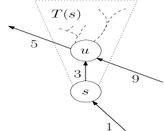
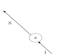
Figure 1: To the left, we have tree $T(s)$. To the right we contract $T(s)$ and identify the supervertex with $s$. We update the weight of outgoing edges and remove the edges ingoing in $T(s)-s$.

A small but important implementation detail, we point out, is that while the pseudocode specifies that Algorithm 1 initializes each graph $H_{J}$ as a copy of $H_{I}$ in Algorithm 1, the data structure technically only copies the subset $\{r_{j_{1}},r_{j_{1}+1},\ldots,r_{j_{2}}\}$ of the vertices on $f_{\infty}$. By our earlier simplifying assumption, the omitted roots are not part of any shortest path tree in any recursive calls involving sub-intervals of $J$ so omitting them will not affect the behaviour of MSSP. Including the entire face $f_{\infty}$ in all recursive calls, however, eases the presentation of proofs.

Query.

The query procedure is straight-forward and given by Algorithm 2.

1

1

Procedure Query($u,j,I=[i_{1},i_{2}]$)

2       if $j=i_{1}$ or $j=i_{2}$ then  return $d_{T_{I,j}}(r_{j},u)$

3       $i\leftarrow\lfloor\frac{i_{1}+i_{2}}{2}\rfloor$

4       if $j\leq i$ then  return Query(${s_{[i_{1},i]}(u),j,[i_{1},i]}$) $+~{}\delta_{[i_{1},i]}(u)$

5       else  return Query(${s_{[i,i_{2}]}(u),j,[i,i_{2}]}$) $+~{}\delta_{[i,i_{2}]}(u)$

6      

Algorithm 2 The procedure to query $d_{G}(b_{j},u)$. Initial call is $\textsc{Query}(u,j,[0,|V_{\infty}|-1])$.

5 Analysis

We now prove the following theorem which summarizes our main result.

Let $G$ be an $n$-vertex planar embedded graph and $f_{\infty}$ be the infinite face on $G$. Then we can build a data structure answering the distance $d_{G}(b_{j},u)$ between any vertex $b_{j}\in f_{\infty}$ and any other vertex $u$ in $O(\log|f_{\infty}|)$ time, using procedure $\textsc{Query}(u,j,[0,|f_{\infty}|-1]))$. Preprocessing requires $O(n\log|f_{\infty}|)$ time and space, using procedure MSSP$([0,|f_{\infty}|-1],G)$.

Correctness.

Let us first prove correctness of the data structure. We start with the observation that no edge incident to $f_{\infty}$ is ever contracted.

For any graph $H_{I}$, no edge incident to $f_{\infty}$ is contracted by MSSP$(I,H_{I})$.

Proof.

This is immediate from our assumption that no shortest path has an ingoing edge to a vertex of $f_{\infty}$ since only edges shared by shortest path trees are contracted. ∎

Next, we prove a lemma and its corollary that roughly show that the contractions made in Procedure MSSP do not destroy shortest paths from roots on sub-intervals $J$ of $f_{\infty}$. The reader is referred to Figure 2 for intuition.

Figure 2: The shortest path trees from $r_{j_{1}}$ and $r_{j_{2}}$ share the dashed edges denoting the tree $T(s)$ containing $u$. The shortest $r_{j_{1}}$-to-$s$, $r_{j_{2}}$-to-$s$ paths and the subpath from $r_{j_{2}}$ to $r_{j_{1}}$ in clockwise order along $f_{\infty}$ define $C$ (fat line). As $v,v_{1},v_{2}$ are in clockwise order around $s$, $T(s)-s$ is in $R$. For $j\in[j_{1},j_{2}]$, any $r_{j}$-to-$u$ path intersects either the shortest $r_{j_{1}}$-to-$s$ or the shortest $r_{j_{2}}$-to-$s$ path.

We first need the following simple claim. For any invocation of MSSP$(I,H_{I})$, any $i\in I$, and any $u\in V(H_{I})-V_{\infty}$, some $r_{i}$-to-$u$ path exists in $H_{I}[(V(H_{I})-V_{\infty})\cup\{r_{i}\}]$.

Proof.

By assumption, an $r_{i}$-to-$u$ path exists in $G[(V-V_{\infty})\cup\{r_{i}\}]$. The claim now follows since $H_{I}$ is obtained from contractions in $G\setminus V_{\infty}$ by Section 5. ∎

Consider any invocation of MSSP$(I,H_{I})$ where $H_{I}$ has unique shortest paths from $r_{i}$ for each $i\in I$. Then for each vertex $u\in T(s)\in\mathcal{T}$ in Line 1 and for each $j\in J$, $P_{H_{I}}[s,u]\subseteq P_{H_{I}}[r_{j},u]$.

Proof.

The proof is trivial for $u=s$, thus we assume $u\neq s$. Now consider paths $P_{T_{I,j_{1}}}[r_{j_{1}},s]$ and $P_{T_{I,j_{2}}}[r_{j_{2}},s]$. Both paths exist by Section 5. By uniqueness of shortest paths in $H_{I}$, they share only vertex $s$.

Next, consider the concatenation $P[j_{1},j_{2}]$ of $P_{T_{I,j_{1}}}[r_{j_{1}},s]$ and the reverse of $P_{T_{I,j_{2}}}[r_{j_{2}},s]$. From the above, $P[j_{1},j_{2}]$ is simple. Further, consider the concatenation $C$ of $P[j_{1},j_{2}]$ and the path segment $F_{\infty}[r_{j_{2}},r_{j_{1}}]$ from $r_{j_{2}}$ to $r_{j_{1}}$ in clockwise order around $f_{\infty}$. We note that $C$ is a cycle. As $f_{\infty}$ is simple, so is $F_{\infty}[r_{j_{2}},r_{j_{1}}]$, and by our simplifying assumption for shortest paths and Section 5, $P[j_{1},j_{2}]$ only intersects $f_{\infty}$ in vertices $r_{j_{1}}$ and $r_{j_{2}}$. Thus, $C$ is a simple directed cycle.

By the Jordan curve theorem, $C$ partitions the plane into two regions. One region, denoted $R$, is the region to the right when walking along $C$. $T(s)-s$ does not intersect the simple curve $P[j_{1},j_{2}]$ since $H_{I}$ is a planar embedded graph and since shortest paths are simple. It also does not intersect $F_{\infty}[r_{j_{2}},r_{j_{1}}]$ as there are no ingoing edges to $f_{\infty}$ in $G_{\infty}$ (and $f_{\infty}$ is preserved in contractions by Section 5). Since for each child $v$ of $s$ in $T(s)$, the edges $(s,v),(s,\pi_{T_{I,j_{1}}}(s)),(s,\pi_{T_{I,j_{2}}}(s))$ are clockwise around $s$, children of $s$ are contained in $R$, and hence so is $T(s)-s$.

By the choice of $F_{\infty}[r_{j_{2}},r_{j_{1}}]$, $r_{j}$ does not belong to $R$ so $P_{H_{I}}[r_{j},u]$ intersects $C$. Since $u\notin F_{\infty}[r_{j_{2}},r_{j_{1}}]$ and since there is no edge $(a,b)$ of $H_{I}$ with $a\notin V_{\infty}$ and $b\in V_{\infty}$, $P_{H_{I}}[r_{j},u]$ cannot intersect $F_{\infty}[r_{j_{2}},r_{j_{1}}]-\{r_{j_{1}},r_{j_{2}}\}$ so it must intersect $C$ in $P[j_{1},j_{2}]$ and hence intersect either $P_{T_{I,j_{1}}}[r_{j_{1}},s]$ or $P_{T_{I,j_{2}}}[r_{j_{2}},s]$; assume the former (the other case is symmetric). Then $P_{H_{I}}[r_{j},u]$ intersects $P_{T_{I,j_{1}}}[r_{j_{1}},s]$ in some vertex $x$. Since shortest paths are unique, the subpath of $P_{H_{I}}[r_{j},u]$ from $x$ to $u$ must then equal $P_{T_{I,j_{1}}}[x,u]$ and since $s$ is on this subpath, the lemma follows. ∎

Let $H_{J}$ be one of the graphs obtained in a call to MSSP$(I,H_{I})$ by contracting edges $E^{\prime}$ in $H_{I}$. Then, for each $j\in J$ and each $u\in V(H_{J})-V_{\infty}$, $P_{H_{J}}[r_{j},u]=P_{H_{I}}[r_{j},u]/E^{\prime}$ is unique and $w_{H_{J}}(P_{H_{J}}[r_{j},u])=w_{H_{I}}(P_{H_{I}}[r_{j},u])$.

Proof.

By Section 5, when contracting $P_{H_{I}}[r_{j},u]$ by $E^{\prime}$, no edge on the path has its weight increased to $\infty$. Further, for any edge $(x,y)\in P_{H_{J}}[r_{j},u]$, either $(x,y)$ existed already in $H_{I}$ in which case its weight is unchanged, or $(x,y)$ originated from an edge $(w,y)$ for $w\in T(x)$. But in the latter case, $P_{H_{I}}[r_{j},u]$ contains $P_{H_{I}}[x,w]$ followed by $(w,y)$ (Section 5), whose weight is $d_{H_{I}}(x,w)+w_{H_{I}}(w,y)=d_{H_{J}}(x,y)$. Thus $w_{H_{J}}(P_{H_{J}}[r_{j},u])\leq w_{H_{I}}(P_{H_{I}}[r_{j},u])$.

It is straight-forward to see that distances in $H_{J}$ also have not decreased since edges affected by the contractions obtain weights corresponding to paths in $H_{I}$ between their endpoints or weight $\infty$. Uniqueness follows since two different shortest paths in $H_{J}$ from $r_{j}$ to a vertex $u$ would imply two different shortest paths between the same pair in $H_{I}$ and, by an inductive argument, also in $G$, contradicting our assumption of uniqueness. ∎

In fact, Section 5 is all we need to prove correctness of our algorithm.

The call Query$(u,j,I=[i_{1},i_{2}])$ outputs $d_{H_{I}}(r_{j},u)$, for $u\in V(H_{I})-V_{\infty}$. In particular, Query$(u,j,I=[0,|V_{\infty}|-1])$ outputs $d_{G}(r_{j},u)$ for $u\in V$.

Proof.

We prove this by induction on $i_{2}-i_{1}$. If $j\in\{i_{1},i_{2}\}$ then Query$(u,j,[i_{1},i_{2}])$ directly returns $d_{T_{I,j}}(r_{j},u)=d_{H_{I}[(H_{I}-V_{\infty})\cup\{r_{j}\}]}(r_{j},u)$. This, in turn, is equal to $d_{H_{I}}(r_{j},u)$ as the only $r_{j}$-to-$u$ paths not considered contain an $\infty$-weight edge with both endpoints in $V_{\infty}$. Therefore the claim holds if $0\leq i_{2}-i_{1}\leq 1$ as $j\in\{i_{1},i_{2}\}$ is implied.

For the inductive step, we thus assume $i_{2}-i_{1}>1$ and $i_{1}<j<i_{2}$. Let $i=\lfloor\frac{i_{1}+i_{2}}{2}\rfloor$ and assume $j\leq i$ (the case $j>i$ is symmetric). Let $s$ be the vertex in $H_{I}$ such that $u\in T(s)$, where possibly $u=s$ (Line 1). By the inductive hypothesis, Query$(u,j,[i_{1},i])$ returns Query$(s_{[i_{1},i]}(u),j,[i_{1},i])$$+\delta_{[i_{1},i]}(u)=d_{H_{[i_{1},i]}}(r_{j},s)+d_{T(s)}(s,u)$. By Section 5, $d_{H_{[i_{1},i]}}(r_{j},s)=d_{H_{I}}(r_{j},s)$. By definition of $T(s)$, $d_{T(s)}(s,u)$ is a suffix of $d_{H_{I}}(r_{i_{1}},u)$, meaning that $d_{T(s)}(s,u)=d_{H_{I}}(s,u)$. Finally, by Lemma 5 the shortest path in $H_{I}$ from $r_{j}$ to $u$ contains $s$, therefore $d_{H_{[i_{1},i],j}}(r_{j},s)+d_{T(s)}(s,u)=d_{H_{I}}(r_{j},s)+d_{H_{I}}(s,u)=d_{H_{I}}(r_{j},u)$. ∎

Bounding Time and Space.

The following Lemma captures our key insight about Algorithm 1 that ensures that the algorithm can be implemented efficiently.

Let $\mathcal{I}_{h}$ be the set of all intervals $I$, such that $\textsc{MSSP}(I,H_{I})$ is executed at recursion level $h$ after invoking $\textsc{MSSP}([0,|V_{\infty}|-1],G)$.

For each edge $e=(u,v)\in E(G)$ and recursion level $h$, there are only $O(1)$ intervals $I\in\mathcal{I}_{h}$ for which there exists an $i\in I$ such that the SSSP tree $T_{I,i}$ from $r_{i}$ in $H_{I}$ contains $e$.

Proof.

We use induction on $h$. As $\mathcal{I}_{0}=\{[0,|V_{\infty}|-1]\}$ the Lemma is trivial for level $h=0$. For $h\geq 0$, we show the inductive step $h\mapsto h+1$. Each interval $[i_{1},i_{2}]=I\in\mathcal{I}_{h}$ satisfies exactly one of the following conditions:

• $\forall i\in I,e\not\in E(T_{I,i})$: Consider a recursive call $\textsc{MSSP}(J,H_{J})$ for $J\subseteq I$ issued in $\textsc{MSSP}(I,H_{I})$ where $H_{J}$ was obtained by contracting some edge set $E^{\prime}$ in $H_{I}$. By Section 5, for any $j\in J$, $P_{H_{J}}[r_{j},u]=P_{H_{I}}[r_{j},u]/E^{\prime}$, but due to our condition and $j\in I$, this path cannot contain $e$.

• $\forall i\in I,e\in E(T_{I,i})$: Let $\mathcal{I}_{h}^{\prime}$ be the subset of intervals $I\in\mathcal{I}_{h}$ satisfying this condition and let $\mathcal{J}_{h+1}^{\prime}$ be the intervals $J\in\mathcal{I}_{h+1}$ contained in such intervals $I$. We show that for at most one $I\in\mathcal{I}_{h}^{\prime}$ does there exist a sub-interval $J\in\mathcal{J}_{h+1}^{\prime}$ where $e$ has not been contracted in $H_{J}$.

  Consider the set $\mathcal{P}$ of shortest paths in $G$ from each endpoint of an interval in $\mathcal{J}_{h+1}^{\prime}$ to vertex $u$. Their union is a tree $T$ with leaves in $V_{\infty}$ and with all edges directed towards the root $u$; see the dashed paths in Figure 3. By definition of $\mathcal{I}_{h}^{\prime}$ and $\mathcal{J}_{h+1}^{\prime}$ and by repeated applications of Corollary 5 to intervals containing $I$ at recursion levels less than $h$, each shortest path in $\mathcal{P}$ is a subpath of a shortest path to $v$ in $G$ with $(u,v)$ as the final edge. Since shortest paths are simple, $v$ cannot belong to $T$.

  Now, consider an interval $J=[j_{1},j_{2}]\in\mathcal{J}_{h+1}^{\prime}$. Let $x$ be the nearest common ancestor of $r_{j_{1}}$ and $r_{j_{2}}$ in $T$. Let $C_{J}$ be the simple directed cycle obtained by the concatenation of the path $T[r_{j_{1}},x]$, the reverse of the path $T[r_{j_{2}},x]$, and the path from $r_{j_{2}}$ to $r_{j_{1}}$ in counter-clockwise order along $f_{\infty}$. Let $R_{J}$ be the open region of the plane to the left of $C_{J}$. Note that shortest path $P_{G}[x,v]$ is $T[x,u]$ concatenated with $(u,v)$. If $P_{G}[x,v]$ emanates to the left of $C_{J}$ at $x$ then since a shortest path cannot cross itself, $v$ must belong to $R_{J}$. In this case, $v$ cannot also belong to $R_{J^{\prime}}$ for any other $J^{\prime}\in\mathcal{J}_{h+1}^{\prime}$ since these regions are pairwise disjoint; see Figure 3. Hence, there is at most one choice of $J$ where $P_{G}[x,v]$ emanates to the left of $C_{J}$ at $x$.

  Using the above notation, it now suffices to show that for an interval $J=[j_{1},j_{2}]\in\mathcal{J}_{h+1}^{\prime}$ where $P_{G}[x,v]$ emanates to the right of $C_{J}$ at $x$, $e$ is contracted in $H_{J}$.

  Let $I\in\mathcal{I}_{h}^{\prime}$ be the parent interval containing $J$. By Corollary 5, $P_{H_{I}}[r_{j_{1}},v]$ is obtained from $P_{G}[r_{j_{1}},v]$ by edge contractions and $P_{H_{I}}[r_{j_{2}},v]$ is obtained similarly from $P_{G}[r_{j_{2}},v]$. Let $(u_{1},x)$ resp. $(u_{2},x)$ be the ingoing edge to $x$ in $P_{G}[r_{j_{1}},v]$ resp. $P_{G}[r_{j_{2}},v]$. Edge $(u_{1},x)$ is not in the shortest path tree from $r_{j_{2}}$ in $G$ (otherwise, this tree would have both $(u_{1},x)$ and $(u_{2},x)$ ingoing to $x$) so by Corollary 5, $(u_{1},x)$ is not contracted in $H_{I}$. Similarly, $(u_{2},x)$ is not contracted in $H_{I}$. It follows that $x$ is a vertex in $H_{I}$. Let $(x,y)$ be the first edge on $P_{H_{I}}[x,v]$; this is well-defined since $P_{H_{I}}[x,v]$ contains at least one edge, namely $e$. By the choice of $J$ and by the embedding-preserving properties of contractions, $(x,y)$, $(x,\pi_{T_{I,j_{1}}}(x))$, and $(x,\pi_{T_{I,j_{2}}}(x))$ are clockwise around $x$. Inspecting the description of MSSP$(I,H_{I})$, we see that $P_{H_{I}}[x,v]$ is contained in a tree $T(s)\in\mathcal{T}$ with $s=x$, so $e$ is contracted in $H_{J}$.

  

  Figure 3: Dashed lines are parts of shortest paths $P_{G}[r_{i},v]$ from vertices $r_{i}$ in $f_{\infty}$ to $v$ and form a tree. In the second recursion level we have intervals $I_{0}=[0,2],I_{1}=[2,4],I_{2}=[4,6],I_{3}=[6,8]$. Vertex $x$ is the nearest common ancestor of $r_{2}$ and $r_{4}$ and $R_{[2,4]}$ is the open region to the left of the simple cycle defined by $P_{G}[r_{2},x]$, the reverse of $P_{G}[r_{4},x]$ and the part of $f_{\infty}$ from $r_{4}$ to $r_{2}$ in counter-clockwise order. Regions $R_{[0,2]},R_{[4,6]},R_{[6,8]}$ are defined similarly for the other intervals. Focusing on interval $I_{1}$, let $y$ be the vertex after $x$ towards $u$ in the tree (in this case $y=u$). Edges $(x,y),(x,\pi_{P_{G}[r_{2},u]}(x)),(x,\pi_{P_{G}[r_{4},u]}(x))$ are in counter-clockwise order, implying that $v$ belongs to $R_{[2,4]}$. Since regions are pairwise disjoint, $v$ belongs to no other region.

• $\exists i,i^{\prime}\in I$, $e\in E(T_{I,i})$ and $e\notin E(T_{I,i^{\prime}})$: At most two intervals $I\in\mathcal{I}_{h}$ satisfy this condition which can then spawn at most four intervals in $\mathcal{I}_{h+1}$; this follows from repeated applications of Corollary 5 combined with the easy observation that roots of $f_{\infty}$ whose shortest path trees in $G$ contain $e$ are consecutive in the cyclic ordering along $f_{\infty}$ [18].

∎

The procedure $\textsc{MSSP}([0,|V_{\infty}|-1],G)$ uses $O(n\log|f|)$ time and space. Procedure Query$(u,j,[0,|V_{\infty}|-1])$ has $O(\log|f|)$ running time.

Proof.

For each recursion level $h$, Section 5 implies that each edge $e\in E(G)$ appears in at most $O(1)$ computed SSSP trees. Further, $\sum_{I\in\mathcal{I}_{h}}|I|=O(n)$. Thus, the total number of vertices in $H_{I}$ summed over all $I\in\mathcal{I}_{h}$ is $O(n)$. By sparsity of planar graphs, the total number of edges in these graphs is $O(n)$ as well.

For each such graph $H_{I}$, each SSSP computation in $H_{I}$ can be implemented in time linear in the size of $H_{I}$ by [16]. We also spend this amount time on constructing the graphs $H_{J}$ from $H_{I}$ since the set $E_{shared}\subseteq E(H_{I})$ and associated trees $T(s)$ can be found in $O(1)$ time per edge. Each edge is outgoing from at most one and ingoing to at most one contracted tree and thus possibly changing its weight requires only $O(1)$ time.

It follows that the entire time spent on recursion level $h$ is $O(n)$. Since there are at most $O(\log|f_{\infty}|)$ levels, the first part of the corollary follows. The second part follows since each recursive step in Query takes constant time. ∎

Appendix A Satisfying the input assumptions

In this section, we show how to ensure the input assumptions from the preliminaries.

If $f$ is not the external face $f_{\infty}$, a linear time algorithm can reembed $G$ to ensure this.

Next, we need $f_{\infty}$ to be a simple cycle. We let $b_{0},b_{1},\dots,b_{|f_{\infty}|-1}$ be the vertices on $f_{\infty}$ ordered by their first appearance in the walk along $f_{\infty}$ in clockwise order starting in an arbitrary vertex $b_{0}$, such that the rest of $G$ is on the right when moving on the walk. For each $0\leq i<|f_{\infty}|$, we add a vertex $r_{i}$, and a zero-weight edge $(r_{i},b_{i}^{\prime})$ embedded in the region enclosed by $f_{\infty}$ that does not contain the rest of $G$. Finally, we add edges $(r_{i},r_{i+1\mod|f_{\infty}|})$ in a simple cycle, with infinite weights, and redefine $f_{\infty}$ to be this cycle. It is not hard to see that this transformation can be done in $O(n)$ time and that any query $(b_{i},u)$ in the original graph can be answered by querying $(r_{i},u)$ in the transformed graph.

Let $V_{\infty}=\{r_{0},r_{1},\ldots,r_{|f_{\infty}|-1}$. To ensure the requirement that every $r_{i}\in V_{\infty}$ can reach every vertex of $V\setminus V_{\infty}$ in $G[(V-V_{\infty})\cup\{r_{i}\}]$, we add suitable edges of large finite weight to $G\setminus V_{\infty}$ to make this subgraph strongly connected without violating the embedding of $G$.

Disallowing shortest paths from having edges ingoing to $V_{\infty}$ will not disallow any shortest path from $b_{i}$ in the original graph: each such path can be mapped to a path of the same weight in the transformed graph that only intersects $f_{\infty}$ in $r_{i}$.

Finally, unique shortest paths can be ensured using the deterministic perturbation technique in [10]).

References

- [1] G. Borradaile, P. N. Klein, S. Mozes, Y. Nussbaum, and C. Wulff-Nilsen, Multiple-source multiple-sink maximum flow in directed planar graphs in near-linear time, SIAM J. Comput., 46 (2017), pp. 1280–1303.
- [2] G. Borradaile, P. Sankowski, and C. Wulff-Nilsen, Min st-cut oracle for planar graphs with near-linear preprocessing time, ACM Trans. Algorithms, 11 (2015).
- [3] S. Cabello, E. W. Chambers, and J. Erickson, Multiple-source shortest paths in embedded graphs, SIAM Journal on Computing, 42 (2013), pp. 1542–1571.
- [4] P. Charalampopoulos, P. Gawrychowski, S. Mozes, and O. Weimann, Almost optimal distance oracles for planar graphs, in Proceedings of the 51st Annual ACM SIGACT Symposium on Theory of Computing, 2019, pp. 138–151.
- [5] V. Cohen-Addad, S. Dahlgaard, and C. Wulff-Nilsen, Fast and compact exact distance oracle for planar graphs, in 2017 IEEE 58th Annual Symposium on Foundations of Computer Science (FOCS), IEEE, 2017, pp. 962–973.
- [6] E. Demaine, S. Mozes, C. Sommer, and S. Tazari, Lecture 11 in 6.889: Algorithms for planar graphs and beyond (fall 2011), 2011.
- [7] J. R. Driscoll, N. Sarnak, D. D. Sleator, and R. E. Tarjan, Making data structures persistent, Journal of computer and system sciences, 38 (1989), pp. 86–124.
- [8] D. Eisenstat and P. N. Klein, Linear-time algorithms for max flow and multiple-source shortest paths in unit-weight planar graphs, in Proceedings of the forty-fifth annual ACM symposium on Theory of computing, 2013, pp. 735–744.
- [9] J. Erickson, Lecture 14 in cs 598 jge: One-dimensional computational topology, 2020.
- [10] J. Erickson, K. Fox, and L. Lkhamsuren, Holiest minimum-cost paths and flows in surface graphs, in Proceedings of the 50th Annual ACM SIGACT Symposium on Theory of Computing, STOC 2018, Los Angeles, CA, USA, June 25-29, 2018, I. Diakonikolas, D. Kempe, and M. Henzinger, eds., ACM, 2018, pp. 1319–1332.
- [11] J. Fakcharoenphol and S. Rao, Planar graphs, negative weight edges, shortest paths, and near linear time, Journal of Computer and System Sciences, 72 (2006), pp. 868–889.
- [12] V. Fredslund-Hansen, S. Mozes, and C. Wulff-Nilsen, Truly subquadratic exact distance oracles with constant query time for planar graphs, arXiv preprint arXiv:2009.14716, (2020).
- [13] P. Gawrychowski and A. Karczmarz, Improved bounds for shortest paths in dense distance graphs, in 45th International Colloquium on Automata, Languages, and Programming (ICALP 2018), Schloss Dagstuhl-Leibniz-Zentrum fuer Informatik, 2018.
- [14] P. Gawrychowski, S. Mozes, O. Weimann, and C. Wulff-Nilsen, Better tradeoffs for exact distance oracles in planar graphs, in Proceedings of the 29th Annual ACM-SIAM Symposium on Discrete Algorithms, no. SODA ‘18, 2018, pp. 515–529.
- [15] R. Geisberger, P. Sanders, D. Schultes, and D. Delling, Contraction hierarchies: Faster and simpler hierarchical routing in road networks, in International Workshop on Experimental and Efficient Algorithms, Springer, 2008, pp. 319–333.
- [16] M. R. Henzinger, P. N. Klein, S. Rao, and S. Subramanian, Faster shortest-path algorithms for planar graphs, J. Comput. Syst. Sci., 55 (1997), pp. 3–23.
- [17] G. F. Italiano, Y. Nussbaum, P. Sankowski, and C. Wulff-Nilsen, Improved algorithms for min cut and max flow in undirected planar graphs, in Proceedings of the Forty-Third Annual ACM Symposium on Theory of Computing, STOC ’11, New York, NY, USA, 2011, Association for Computing Machinery, p. 313–322.
- [18] P. N. Klein, Multiple-source shortest paths in planar graphs, in Proceedings of the Sixteenth Annual ACM-SIAM Symposium on Discrete Algorithms, SODA 2005, Vancouver, British Columbia, Canada, January 23-25, 2005, SIAM, 2005, pp. 146–155.
- [19] P. N. Klein and S. Mozes, Optimization algorithms for planar graphs, preparation, manuscript at http://planarity. org, (2014).
- [20] Y. Long and S. Pettie, Planar distance oracles with better time-space tradeoffs, in Proceedings of the 2021 ACM-SIAM Symposium on Discrete Algorithms, SODA’21, 2021, pp. 2517–2537.
- [21] Y. Long and S. Pettie, Planar distance oracles with better time-space tradeoffs, in Proceedings of the 2021 ACM-SIAM Symposium on Discrete Algorithms (SODA), SIAM, 2021, pp. 2517–2537.
- [22] S. Mozes, Y. Nussbaum, and O. Weimann, Faster shortest paths in dense distance graphs, with applications, Theoretical Computer Science, 711 (2018), pp. 11–35.
- [23] S. Mozes and C. Wulff-Nilsen, Shortest paths in planar graphs with real lengths in o (nlog 2 n/loglogn) time, in European Symposium on Algorithms, Springer, 2010, pp. 206–217.
- [24] R. E. Tarjan and R. F. Werneck, Dynamic trees in practice, Journal of Experimental Algorithmics (JEA), 14 (2010), pp. 4–5.
- [25] M. Thorup, Compact oracles for reachability and approximate distances in planar digraphs, Journal of the ACM (JACM), 51 (2004), pp. 993–1024.