Computing Gröbner bases of ideal interpolation

Abstract

We present algorithms for computing the reduced Gröbner basis of the vanishing ideal of a finite set of points in a frame of ideal interpolation. Ideal interpolation is defined by a linear projector whose kernel is a polynomial ideal. In this paper, we translate interpolation condition functionals into formal power series via Taylor expansion, then the reduced Gröbner basis is read from formal power series by Gaussian elimination. Our algorithm has a polynomial time complexity, an example suggests that our method compares favorably with MMM algorithm in some special cases.

1 Introduction

Let $\mathbb{F}$ be either the real field $\mathbb{R}$ or the complex field $\mathbb{C}$. Polynomial interpolation is to construct a polynomial $g$ belonging to a finite-dimensional subspace of $\mathbb{F}[{\bf X}]$ that agrees with a given function $f$ at the data set, where $\mathbb{F}[{\bf X}]:=\mathbb{F}[x_{1},x_{2},\dots,x_{d}]$ denotes the polynomial ring in $d$ variables over the field $\mathbb{F}$.

For studying multivariate polynomial interpolation, Birkhoff [1] introduced the definition of ideal interpolation. Ideal interpolation is defined by a linear projector whose kernel is a polynomial ideal. In ideal interpolation [11], the interpolation condition functionals at an interpolation point $\boldsymbol{\theta}\in\mathbb{F}^{d}$ can be described by a linear space ${\rm span}\{\delta_{\boldsymbol{\theta}}\circ P(D),P\in P_{\boldsymbol{\theta}}\}$, where $P_{\boldsymbol{\theta}}$ is a $D$-invariant polynomial subspace, $\delta_{\boldsymbol{\theta}}$ is the evaluation functional at $\boldsymbol{\theta}$ and $P(D)$ is the differential operator induced by $P$. The classical examples of ideal interpolation are Lagrange interpolation and univariate Hermite interpolation.

For an ideal interpolation, suppose that $\Delta$ is the finite set of interpolation condition functionals. Then the set of all polynomials that vanish at $\Delta$ constitutes a 0-dimensional ideal, which is denoted by $I(\Delta)$, namely,

$$I(\Delta):=\{f\in\mathbb{F}[{\bf X}]:L(f)=0,\forall L\in\Delta\}.$$

We refer the readers to [11] and [13] for more details about ideal interpolation.

Gröbner bases [9], introduced by Buchberger [2] in 1965, have been applied successfully in various fields of mathematics and to many types of problems. There are several methods for computing Gröbner bases of vanishing ideals. For any point set $\Theta\subset\mathbb{F}^{d}$ and any fixed monomial order, BM algorithm [3] yields the reduced Gröbner basis and a reducing interpolation Newton basis for a $d$-variate Lagrange interpolation on $\Theta$. BM algorithm computes the vanishing ideal of a finite set of points (in affine space) without multiplicities. [5] presents a variant of BM algorithm which is more effective for the computation over $\mathbb{Q}$, and also considers the case that the set of points is in the projective space. As a generalization of univariate Newton interpolation, Farr and Gao [6] give an algorithm that computes the reduced Gröbner basis for vanishing ideals under any monomial order. Applying Taylor expansions to the original algorithm, Farr and Gao’s method can be applied to compute the vanishing ideal when the interpolation points have multiplicities, but the multiplicity set needs to be a delta set in $\mathbb{N}^{d}$. In this paper, we consider the more general case that the multiplicity space of each point just needs to be closed under differentiation. To avoid solving linear equations, Lederer [7] gives an algorithm to compute the Gröbner basis of an arbitrary finite set of points under lexicographic order by induction over the dimension $d$. Jiang, Zhang and Shang [8] give an algorithm for computing the Gröbner basis of a single point ideal interpolation.

To the best of our knowledge, for the general case of ideal interpolation, computing the reduced Gröbner basis needs to solve a linear system. In 1993, Marinari, Möller and Mora [4] constructed a linear system based on a Vandermonde-like matrix, and gave an algorithm (MMM algorithm) to compute general 0-dimensional ideals by Gaussian elimination. MMM algorithm has a polynomial time complexity and is one of the most famous algorithms in recent years.

Throughout the paper, $\mathbb{N}$ denotes the set of nonnegative integers. Let $\mathbb{N}^{d}:=\{(\alpha_{1},\alpha_{2},\dots,\alpha_{d}):\alpha_{i}\in\mathbb{N}\}$. For $\boldsymbol{\alpha}=(\alpha_{1},\alpha_{2},\dots,\alpha_{d})\in\mathbb{N}^{d}$, define $\boldsymbol{\alpha}!:=\alpha_{1}!\alpha_{2}!\cdots\alpha_{d}!$ and denote by ${\bf X}^{\boldsymbol{\alpha}}$ the monomial $x_{1}^{\alpha_{1}}x_{2}^{\alpha_{2}}\cdots x_{d}^{\alpha_{d}}$. Let $\{{\bf X}^{\boldsymbol{\alpha_{1}}},{\bf X}^{\boldsymbol{\alpha_{2}}},\dots,{\bf X}^{\boldsymbol{\alpha_{n}}}\}$ be a finite set of monomials and $\{L_{i}:\mathbb{F}[{\bf X}]\to\mathbb{F},i=1,2,\dots,n\}$ be a finite set of linearly independent functionals. We can treat the matrix

$$\left({\begin{array}[]{*{20}{c}}{{L_{1}}({{\bf X}^{\boldsymbol{\alpha_{1}}}})}&{{L_{1}}({{\bf X}^{\boldsymbol{\alpha_{2}}}})}&\cdots&{{L_{1}}({{\bf X}^{\boldsymbol{\alpha_{n}}}})}\\ {{L_{2}}({{\bf X}^{\boldsymbol{\alpha_{1}}}})}&{{L_{2}}({{\bf X}^{\boldsymbol{\alpha_{2}}}})}&\cdots&{{L_{2}}({{\bf X}^{\boldsymbol{\alpha_{n}}}})}\\ \vdots&\vdots&&\vdots\\ {{L_{n}}({{\bf X}^{\boldsymbol{\alpha_{1}}}})}&{{L_{n}}({{\bf X}^{\boldsymbol{\alpha_{2}}}})}&\cdots&{{L_{n}}({{\bf X}^{\boldsymbol{\alpha_{n}}}})}\end{array}}\right)$$

as a Vandermonde-like matrix.

In this paper, we give algorithms to compute the reduced Gröbner basis by Gaussian elimination. Our major idea is based on the formal power series appeared in [12]. In that paper, de Boor and Ron deduced excellent properties for the basis of interpolation they computed as the least degree forms of formal power series. In this paper, we focus on extracting the reduced Gröbner basis from interpolation condition functionals. We translate interpolation condition functionals into formal power series via Taylor expansion, then the reduced Gröbner basis is read from formal power series by Gaussian elimination.

The paper is organized as follows. The preliminary is in Section 2. The algorithm for computing the “reverse” reduced team is in Section 3. The method to find the quotient ring basis is in Section 4. The algorithms for computing the reduced Gröbner bases are presented in Section 5. A special example is discussed in Section 6.

2 Preliminary

A polynomial $P\in\mathbb{F}[{\bf X}]$ can be considered as the formal power series

$$P=\sum_{\boldsymbol{\alpha}\in\mathbb{N}^{d}}\hat{P}(\boldsymbol{\alpha}){\bf X}^{\boldsymbol{\alpha}},$$

where $\hat{P}(\boldsymbol{\alpha})$ are the coefficients in the polynomial $P$.

$P(D):=P(D_{x_{1}},D_{x_{2}},\dots,D_{x_{d}})$ is the differential operator induced by the polynomial $P$, where $D_{x_{j}}:=\frac{\partial}{\partial x_{j}}$ is the differentiation with respect to the $j$th variable, $j=1,2,\dots,d$.

Define $D^{\boldsymbol{\alpha}}:=D_{x_{1}}^{\alpha_{1}}D_{x_{2}}^{\alpha_{2}}\cdots D_{x_{d}}^{\alpha_{d}}$. The differential polynomial can be rewritten as

$$P(D)=\sum_{\boldsymbol{\alpha}\in\mathbb{N}^{d}}\hat{P}(\boldsymbol{\alpha})D^{\boldsymbol{\alpha}}.$$

Given a monomial order $\prec$, the least monomial of the polynomial $P$ w.r.t. $\prec$ is defined by

$${\rm lm}(P):=\min_{\prec}\{{\bf X}^{\boldsymbol{\alpha}}\mid\hat{P}(\boldsymbol{\alpha})\neq 0\}.$$

Definition 1

We denote by $\Lambda\{P_{1},P_{2},\dots,P_{n}\}$ the set of all monomials that occur in the polynomials $P_{1},P_{2},\dots,P_{n}$ with nonzero coefficients.

For example, let $P_{1}=1,P_{2}=x,P_{3}=\frac{1}{2}x^{2}+y$, then

$$\Lambda\{P_{1},P_{2},P_{3}\}=\{1,x,y,x^{2}\}.$$

Definition 2

Given a monomial order $\prec$, a set of linearly independent polynomials $\{P_{1},P_{2},\dots,P_{n}\}\subset\mathbb{F}[{\bf X}]$ is called a “reverse” reduced team w.r.t.$\prec$, if

1. the coefficient of the least monomial of the polynomial $P_{i},1\leq i\leq n$ is 1;

2. ${\rm lm}(P_{i})\not\in\Lambda\{P_{j}\},i\neq j,1\leq i,j\leq n$.

For example, given the monomial order $\mathrm{grlex}(z\prec y\prec x)$,

$$\{1,x,\frac{1}{2}x^{2}+y,\frac{1}{6}x^{3}-x^{2}+xy\},~{}~{}\{1,y+z,x\},~{}~{}\{1,x+z,-x+y\}$$

are “reverse” reduced teams w.r.t. $\prec$.

3 Computing a “reverse” reduced team by Gaussian elimination

Let $T$ and $\bar{T}$ be two sets of monomials in $\mathbb{F}[{\bf X}]$, the notation $\bar{T}-T$ is reserved for the set $\{t:t\in\bar{T},t\notin T\}$.

Given a monomial order $\prec$, $P_{1},P_{2},\dots,P_{n}\in\mathbb{F}[{\bf X}]$ are linearly independent polynomials. Algorithm 1 yields a “reverse” reduced team w.r.t. $\prec$.

1:  Input: A monomial order $\prec$.

2:             Linearly independent polynomials $P_{1},P_{2},\dots,P_{n}\in\mathbb{F}[{\bf X}]$.

3:  Output: $\{P_{1}^{*},P_{2}^{*},\dots,P_{n}^{*}\}$, a “reverse” reduced team w.r.t. $\prec$.

4:  //Initialization

5:  ${\rm{List}}:=\Lambda\{P_{1},P_{2},\dots,P_{n}\}$;

16:  ${\bf X}^{\boldsymbol{\alpha}}:=\rm{min}(\rm{List},\prec)$;

7:  ${\rm{U}}:=(\hat{P}_{1}(\boldsymbol{\alpha}),\hat{P}_{2}(\boldsymbol{\alpha}),\dots,\hat{P}_{n}(\boldsymbol{\alpha}))^{\prime}$;

8:  $\rm{List}:=\rm{List}-\{{\bf X}^{\boldsymbol{\alpha}}\}$;

9:  while $\rm{List}\neq\emptyset$  do

10:     ${\bf X}^{\boldsymbol{\alpha}}:=\rm{min}(\rm{List},\prec)$;

11:     $v:=(\hat{P}_{1}(\boldsymbol{\alpha}),\hat{P}_{2}(\boldsymbol{\alpha}),\dots,\hat{P}_{n}(\boldsymbol{\alpha}))^{\prime}$;

12:     ${\rm{U}}:=[{\rm{U}},v]$;

213:     $\rm{List}:=\rm{List}-\{{\bf X}^{\boldsymbol{\alpha}}\}$;

314:  end while

15:  //Computing

16:  $\rm{U}^{*}=\rm{rref}[\rm{U}]$; (reduced row echelon form)

17:  ${\rm{List}}:=\Lambda\{P_{1},P_{2},\dots,P_{n}\}$;

18:  for $i=1:n$ do

19:     $P_{i}^{*}={\rm{U}}^{*}(i,:)\cdot(\rm{List},\prec)^{\prime}$;

20:  end for

21:  return  $\{P_{1}^{*},P_{2}^{*},\dots,P_{n}^{*}\}$.

Algorithm 1 A “reverse” reduced team w.r.t. $\prec$

For example, given the monomial order $\mathrm{grlex}(y\prec x)$, $P_{1}=1$, $P_{2}=x$,$P_{3}=\frac{1}{2}x^{2}+y$, $P_{4}=\frac{1}{6}x^{3}+xy+2y$. We get

$$({\rm{List}},\prec)=(1,y,x,xy,x^{2},x^{3}),$$

$${\rm{U}}=\left({\begin{array}[]{*{20}{c}}1&0&0&0&0&0\\ 0&0&1&0&0&0\\ 0&1&0&0&{1/2}&0\\ 0&2&0&1&0&{1/6}\end{array}}\right),$$

$${{\rm{U}}^{*}}=\left({\begin{array}[]{*{20}{c}}1&0&0&0&0&0\\ 0&1&0&0&{1/2}&0\\ 0&0&1&0&0&0\\ 0&0&0&1&-1&{1/6}\end{array}}\right),$$

${P_{1}}^{*}=1$,   ${P_{2}}^{*}=\frac{1}{2}x^{2}+y$,   ${P_{3}}^{*}=x$,   ${P_{4}}^{*}=\frac{1}{6}x^{3}-x^{2}+xy$.

4 Interpolation monomial basis and quotient ring basis

Given interpolation conditions $\Delta={\rm span}\{L_{1},L_{2},\dots,L_{n}\}$, where $L_{1},L_{2},\dots,L_{n}$ are linearly independent functionals. Let $T=\{{\bf X}^{\boldsymbol{\alpha_{1}}},{\bf X}^{\boldsymbol{\alpha_{2}}},\dots,{\bf X}^{\boldsymbol{\alpha_{n}}}\}$ be a set of monomials, then $T$ is an interpolation monomial basis for $\Delta$ if the Vandermonde-like matrix ( applying the data map $\{L_{i}:i=1,2,\dots,n\}$ to the column map $\{{\bf X}^{\boldsymbol{\alpha_{j}}}:j=1,2,\dots,n\}$) is non-singular.

Definition 3

Let $T$ and $\bar{T}$ be two sets of monomials in $\mathbb{F}[{\bf X}]$ with $\bar{T}-T\neq\emptyset$ and $T-\bar{T}\neq\emptyset$. Given a monomial order $\prec$, we write $\bar{T}\prec T$, if

$$\max_{\prec}(\bar{T}-T)\prec\max_{\prec}(T-\bar{T}).$$

Definition 4 ($\prec$-minimal monomial basis [10])

Given a monomial order $\prec$ and interpolation conditions $\Delta={\rm span}\{L_{1},L_{2},\dots,L_{n}\}$, where $L_{1},L_{2},\dots,L_{n}$ are linearly independent functionals. Let $T$ be an interpolation monomial basis for $\Delta$, then $T$ is $\prec$-minimal if there exists no interpolation monomial basis $\bar{T}$ for $\Delta$ satisfying $\bar{T}\prec T$.

First, we consider the interpolation problem at the origin.

Lemma 5

Given interpolation conditions $\Delta=\delta_{\bf 0}\circ{\rm span}\{P_{1}(D),P_{2}(D),\dots,P_{n}(D)\}$, where $P_{1},P_{2},\dots,P_{n}\in\mathbb{F}[{\bf X}]$ are linearly independent polynomials. Let $T=\{{\bf X}^{\boldsymbol{\beta_{1}}},{\bf X}^{\boldsymbol{\beta_{2}}},\dots,{\bf X}^{\boldsymbol{\beta_{n}}}\}$ be an interpolation monomial basis for $\Delta$, then for each $P_{i},1\leq i\leq n$, there exists an ${\bf X}^{\boldsymbol{\alpha_{i}}}\in\Lambda\{P_{i}\}$ satisfying ${\bf X}^{\boldsymbol{\alpha_{i}}}\in T$.

Proof. We will prove this by contradiction. Without loss of generality, we can assume that for every ${\bf X}^{\boldsymbol{\alpha}}\in\Lambda\{P_{1}\}$, ${\bf X}^{\boldsymbol{\alpha}}\not\in T$. It is observed that

$$[\delta_{\bf 0}\circ P_{1}(D)]{\bf X}^{\boldsymbol{\beta_{j}}} =[\delta_{\bf 0}\circ\sum\hat{P_{1}}(\boldsymbol{\alpha})D^{\boldsymbol{\alpha}}]{\bf X}^{\boldsymbol{\beta_{j}}}$$

$$=\sum\hat{P_{1}}(\boldsymbol{\alpha})\underbrace{(\delta_{\bf 0}\circ D^{\boldsymbol{\alpha}}{\bf X}^{\boldsymbol{\beta_{j}}})}_{0}$$

$$=0,\quad 1\leq j\leq n.$$

So the Vandermonde-like matrix has a zero row, and it is singular. It contradicts with the condition that $T=\{{\bf X}^{\boldsymbol{\beta_{1}}},{\bf X}^{\boldsymbol{\beta_{2}}},\dots,{\bf X}^{\boldsymbol{\beta_{n}}}\}$ is an interpolation monomial basis for $\Delta$.     $\Box$

Given interpolation conditions $\Delta=\delta_{\bf 0}\circ{\rm span}\{P_{1}(D),P_{2}(D),\dots,P_{n}(D)\}$, Lemma 5 shows that we need to choose at least one monomial from each $P_{i},1\leq i\leq n$ to form the interpolation monomial basis for $\Delta$.

For $\boldsymbol{\theta}=(\theta_{1},\theta_{2},\dots,\theta_{d})\in\mathbb{F}^{d}$, we denote $\boldsymbol{\theta}{\bf X}:=\sum_{i=1}^{d}\theta_{i}x_{i}$. From Taylor’s formula, we have

$$e^{\boldsymbol{\theta}{\bf X}}=\sum_{j=0}^{\infty}\frac{(\boldsymbol{\theta}{\bf X})^{j}}{j!}.$$

Then, we have

$$\delta_{\boldsymbol{\theta}}=\delta_{\bf 0}\circ e^{\boldsymbol{\theta}D}.$$ (1)

Further more, we get

$$\delta_{\boldsymbol{\theta}}\circ P(D)=\delta_{\bf 0}\circ e^{\boldsymbol{\theta}D}P(D).$$ (2)

This means that an interpolation problem at a nonzero point can be converted into one at the origin.

Theorem 6

For any $\boldsymbol{\theta}\in\mathbb{F}^{d}$, given a monomial order $\prec$ and interpolation conditions $\Delta=\delta_{\boldsymbol{\theta}}\circ{\rm span}\{P_{1}(D),P_{2}(D),\dots,P_{n}(D)\}$. If $\{P_{1},P_{2},\dots,P_{n}\}$ is a “reverse” reduced team w.r.t. $\prec$, then $\{{\rm lm}(P_{1}),{\rm lm}(P_{2}),\dots,{\rm lm}(P_{n})\}$ is the $\prec$-minimal monomial basis for $\Delta$.

Proof. Let ${\tilde{P}_{i}}(D)={e^{\boldsymbol{\theta}D}}P_{i}(D),1\leq i\leq n$. By (2), we have

$$\Delta=\delta_{\boldsymbol{\theta}}\circ{\rm span}\{P_{1}(D),P_{2}(D),\dots,P_{n}(D)\}=\delta_{\bf 0}\circ{\rm span}\{\tilde{P}_{1}(D),\tilde{P}_{2}(D),\dots,\tilde{P}_{n}(D)\}.$$

According to Lemma 5, we choose at least one monomial from each $\tilde{P}_{i},1\leq i\leq n$ to form the interpolation monomial basis. On the other hand, $P_{i},1\leq i\leq n$ are assumed to be linearly independent, which implies that the cardinal number of interpolation monomial basis is $n$. Thus, it is easy to see $\{{\rm lm}(\tilde{P}_{1}),{\rm lm}(\tilde{P}_{2}),\dots,{\rm lm}(\tilde{P}_{n})\}$ is minimal choice w.r.t. $\prec$. We only need to prove $\{{\rm lm}(\tilde{P}_{1}),{\rm lm}(\tilde{P}_{2}),\dots,{\rm lm}(\tilde{P}_{n})\}$ is an interpolation monomial basis for $\Delta$.

Let $P_{i}=\sum\hat{P_{i}}(\boldsymbol{\alpha}){\bf X}^{\boldsymbol{\alpha}}+{\bf X}^{\boldsymbol{\beta_{i}}}$, ${\rm lm}(P_{i})={\bf X}^{\boldsymbol{\beta_{i}}},1\leq i\leq n$. Since $\{P_{1},P_{2},\dots,P_{n}\}$ is a “reverse” reduced team w.r.t. $\prec$, it means

$${\rm lm}(P_{i})\not\in\Lambda\{P_{j}\},\quad i\neq j,1\leq i,j\leq n.$$

Without loss of generality, we can assume that ${\rm lm}(P_{1})\prec{\rm lm}(P_{2})\prec\dots\prec{\rm lm}(P_{n})$, then we have

$${\rm lm}(P_{i})\not\in\Lambda\{\tilde{P}_{j}\},\quad 1\leq i<j\leq n.$$

Notice that ${\rm lm}(\tilde{P}_{i})={\rm lm}(e^{\boldsymbol{\theta}{\bf X}}\cdot P_{i})={\rm lm}(e^{\boldsymbol{\theta}{\bf X}})\cdot{\rm lm}(P_{i})={\rm lm}(P_{i}),1\leq i\leq n$, we have

$${\rm lm}(\tilde{P}_{i})\not\in\Lambda\{\tilde{P}_{j}\},\quad 1\leq i<j\leq n.$$

Thus, we have

$$(\delta_{\bf 0}\circ\tilde{P}_{j}(D))({\rm lm}(\tilde{P}_{i}))=\begin{cases}0,&i<j,\\ \boldsymbol{\beta_{i}}!\neq 0,&i=j,\\ \end{cases}\quad 1\leq i,j\leq n.$$

So the Vandermonde-like matrix is an upper triangular matrix with nonzero diagonal elements, i.e., it is non-singular. It follows that

$$\{{\rm lm}(\tilde{P}_{1}),{\rm lm}(\tilde{P}_{2}),\dots,{\rm lm}(\tilde{P}_{n})\}=\{{\rm lm}(P_{1}),{\rm lm}(P_{2}),\dots,{\rm lm}(P_{n})\}$$

is the $\prec$-minimal monomial basis for $\Delta$.     $\Box$

In ideal interpolation, the $\prec$-minimal monomial basis is equivalent to the monomial basis of the quotient ring w.r.t. $\prec$ [10]. The follwing theorem can be obtained directly by Theorem 6, we list it here without proof.

Theorem 7

For any $\boldsymbol{\theta}\in\mathbb{F}^{d}$, given a monomial order $\prec$ and interpolation conditions $\Delta=\delta_{\boldsymbol{\theta}}\circ{\rm span}\{P_{1}(D),P_{2}(D),\dots,P_{n}(D)\}$. If $\{P_{1},P_{2},\dots,P_{n}\}$ is a “reverse” reduced team w.r.t. $\prec$, then $\{{\rm lm}(P_{1}),{\rm lm}(P_{2}),\dots,{\rm lm}(P_{n})\}$ is the monomial basis of the quotient ring $\mathbb{F}[{\bf X}]/I(\Delta)$ w.r.t. $\prec$.

Now, we show the application of the Theorem 7. For example, given the monomial order $\mathrm{grlex}(y\prec x)$ and ideal interpolation conditions $\Delta=\delta_{(1,2)}\circ{\rm span}\{1,D_{x},\frac{1}{2}D_{x}^{2}+D_{y},\frac{1}{6}D_{x}^{3}+D_{x}D_{y}+2D_{y}\}$. We know $P_{1}=1$, $P_{2}=x$,$P_{3}=\frac{1}{2}x^{2}+y$, $P_{4}=\frac{1}{6}x^{3}+xy+2y$. By Algorithm 1, we have ${P_{1}}^{*}=1$,   ${P_{2}}^{*}=\frac{1}{2}x^{2}+y$,   ${P_{3}}^{*}=x$,   ${P_{4}}^{*}=\frac{1}{6}x^{3}-x^{2}+xy$. By Theorem 7, $\{{\rm lm}(P_{1}^{*}),{\rm lm}(P_{2}^{*}),{\rm lm}(P_{3}^{*}),{\rm lm}(P_{4}^{*})\}=\{1,y,x,xy\}$ is the monomial basis of the quotient ring $\mathbb{F}[{\bf X}]/I(\Delta)$.

5 The algorithms to compute the reduced Gröbner bases

In order to describe algorithms more conveniently, we introduce some notations. Let $\mathbb{F}[[{\bf X}]]$ be the ring of formal power series. Let $T$ be a set of monomials in $\mathbb{F}[{\bf X}]$. For any $f\in\mathbb{F}[[{\bf X}]]$, we denote by

$$\lambda_{T}(f)=\sum\limits_{{\bf X}^{\boldsymbol{\alpha}}\in T}{\hat{f}(\boldsymbol{\alpha}){\bf X}^{\boldsymbol{\alpha}}}$$

a “truncated polynomial”.

Given a monomial order $\prec$ and Lagrange interpolation conditions $\Delta$, Algorithm 2 yields the reduced Gröbner basis for $I(\Delta)$ w.r.t. $\prec$.

1:  Input: A monomial order $\prec$.

2:            The interpolation conditions $\Delta={\rm span}\{\delta_{\boldsymbol{\theta_{1}}},\delta_{\boldsymbol{\theta_{2}}},\dots,\delta_{\boldsymbol{\theta_{n}}}\}$,

13:            where distinct points $\boldsymbol{\theta_{i}}\in\mathbb{F}^{d},i=1,2,\dots,n$.

4:  Output: $\{G_{1},G_{2},\dots,G_{m}\}$, the reduced Gröbner basis for $I(\Delta)$ w.r.t. $\prec$.

25:  //Initialization

6:  $\rm{List}:=\Lambda\{e^{\boldsymbol{\theta_{1}}{\bf X}},e^{\boldsymbol{\theta_{2}}{\bf X}},\dots,e^{\boldsymbol{\theta_{n}}{\bf X}}\}$,  $Q:=\{1\}$,  $G:=\emptyset$;

37:  ${\bf X}^{\boldsymbol{\beta}}:=\rm{min}(\rm{List},\prec)$;

8:  $\rm{U}:=(\hat{e^{\boldsymbol{\theta_{1}}{\bf X}}}(\boldsymbol{\beta}),\hat{e^{\boldsymbol{\theta_{2}}{\bf X}}}(\boldsymbol{\beta}),\dots,\hat{e^{\boldsymbol{\theta_{n}}{\bf X}}}(\boldsymbol{\beta}))^{\prime}$;

49:  $\rm{List}:=\rm{List}-\{{\bf X}^{\boldsymbol{\beta}}\}$;

10:  //Computing

11:  while $\rm{rank}(U)<n$ do

12:     ${\bf X}^{\boldsymbol{\beta}}:=\rm{min}(\rm{List},\prec)$;

513:     $v:=(\hat{e^{\boldsymbol{\theta_{1}}{\bf X}}}(\boldsymbol{\beta}),\hat{e^{\boldsymbol{\theta_{2}}{\bf X}}}(\boldsymbol{\beta}),\dots,\hat{e^{\boldsymbol{\theta_{n}}{\bf X}}}(\boldsymbol{\beta}))^{\prime}$;

14:     if ${\rm{rank}}({\rm{U}},v)>{\rm{rank}}(\rm{U})$ then

15:        ${\rm{U}}:=[{\rm{U}},v]$;

16:        $Q:=Q\cup\{{\bf X}^{\boldsymbol{\beta}}\}$;

17:        $\rm{List}:=\rm{List}-\{{\bf X}^{\boldsymbol{\beta}}\}$;

18:     else

19:        $G:=G\cup\{{\bf X}^{\boldsymbol{\beta}}\}$;

20:        $\rm{List}:=\rm{List}-\{{\rm{multiples~{}of~{}}}{\bf X}^{\boldsymbol{\beta}}\}$;

21:     end if

22:  end while

23:  ${\bf X}^{\boldsymbol{\alpha}}:=\rm{min}(\rm{List},\prec)$;

24:  $G:=G\cup\{{\bf X}^{\boldsymbol{\alpha}}\}$;

25:  $G:=\{{\bf X}^{\boldsymbol{\alpha_{1}}},{\bf X}^{\boldsymbol{\alpha_{2}}},\dots,{\bf X}^{\boldsymbol{\alpha_{m}}}\}$, the set of the leading monomials of the reduced Gröbner basis;

626:  $Q:=\{{\bf X}^{\boldsymbol{\beta_{1}}},{\bf X}^{\boldsymbol{\beta_{2}}},\dots,{\bf X}^{\boldsymbol{\beta_{n}}}\}$, the monomial basis of the quotient ring;

727:  $P_{j}:=\lambda_{G\cup Q}(e^{\boldsymbol{\theta_{j}}{\bf X}}),~{}1\leq j\leq n$;

828:  $\{P_{j}^{*},1\leq j\leq n\}$, a “reverse” reduced team w.r.t. $\prec$, by Algorithm 1;

29:  for $i=1:m$ do

30:     $G_{i}={\bf X}^{\boldsymbol{\alpha_{i}}}-\sum_{j=1}^{n}\left(\frac{(\boldsymbol{\alpha_{i}})!}{(\boldsymbol{\beta_{j}})!}\hat{P}_{j}^{*}(\boldsymbol{\alpha_{i}})\right){\bf X}^{\boldsymbol{\beta_{j}}}$;

31:  end for

32:  return  $\{G_{1},G_{2},\dots,G_{m}\}$.

Algorithm 2 The reduced Gröbner basis (Lagrange interpolation)

In Line 11 and Line 14, we use the skill(recording the reversible matrix used for each calculation) in MMM algorithm to calculate the rank of the matrix by Gaussian elimination. It is obvious that Algorithm 2 terminates. The following theorem shows its correctness.

Theorem 8

The output $\{G_{1},G_{2},\dots,G_{m}\}$ in Algorithm 2 is the reduced Gröbner basis for $I(\Delta)$.

Proof. By (1), $\Delta={\rm span}\{\delta_{\boldsymbol{\theta_{1}}},\delta_{\boldsymbol{\theta_{2}}},\dots,\delta_{\boldsymbol{\theta_{n}}}\}=\delta_{\bf 0}\circ{\rm span}\{e^{\boldsymbol{\theta_{1}}D},e^{\boldsymbol{\theta_{2}}D},\dots,e^{\boldsymbol{\theta_{n}}D}\}$. Suppose that $\{(e^{\boldsymbol{\theta_{1}}{\bf X}})^{*},(e^{\boldsymbol{\theta_{2}}{\bf X}})^{*},\dots,(e^{\boldsymbol{\theta_{n}}{\bf X}})^{*}\}$ is a “reverse” reduced team of $e^{\boldsymbol{\theta_{1}}{\bf X}},e^{\boldsymbol{\theta_{2}}{\bf X}},\dots,e^{\boldsymbol{\theta_{n}}{\bf X}}$. Comparing Line 13 in Algorithm 2 and Line 11 in Algorithm 1, we have $Q=\{{\bf X}^{\boldsymbol{\beta_{1}}},{\bf X}^{\boldsymbol{\beta_{2}}},\dots,{\bf X}^{\boldsymbol{\beta_{n}}}\}=\{{\rm lm}(e^{\boldsymbol{\theta_{1}}{\bf X}})^{*},{\rm lm}(e^{\boldsymbol{\theta_{2}}{\bf X}})^{*},\dots,{\rm lm}(e^{\boldsymbol{\theta_{n}}{\bf X}})^{*}\}$. By Theorem 7, $Q$ is the monomial basis of the quotient ring $\mathbb{F}[{\bf X}]/I(\Delta)$. On the other hand, since $Q$ is a lower set [9], it is easy to check that $G$ is the set of the leading monomials of the reduced Gröbner basis. Thus, we only need to prove that $G_{i}={\bf X}^{\boldsymbol{\alpha_{i}}}-\sum_{j=1}^{n}\left(\frac{(\boldsymbol{\alpha_{i}})!}{(\boldsymbol{\beta_{j}})!}\hat{P}_{j}^{*}(\boldsymbol{\alpha_{i}})\right){\bf X}^{\boldsymbol{\beta_{j}}}$ in Line 30 lies in $I(\Delta)$. Due to $\{P_{1}^{*},P_{2}^{*},\dots,P_{n}^{*}\}$ in Line 28 is a “reverse” reduced team, it follows that ${\rm lm}(P_{j}^{*})={\bf X}^{\boldsymbol{\beta_{j}}}\not\in\Lambda\{P_{k}^{*}\},j\neq k,1\leq j,k\leq n$. Hence, we have

$$\delta_{\bf 0}\circ P_{k}^{*}(D)G_{i}=\delta_{\bf 0}\circ P_{k}^{*}(D)({\bf X}^{\boldsymbol{\alpha_{i}}}-\sum_{j=1}^{n}\left(\frac{(\boldsymbol{\alpha_{i}})!}{(\boldsymbol{\beta_{j}})!}\hat{P}_{j}^{*}(\boldsymbol{\alpha_{i}})\right){\bf X}^{\boldsymbol{\beta_{j}}})$$

$$=\delta_{\bf 0}\circ P_{k}^{*}(D){\bf X}^{\boldsymbol{\alpha_{i}}}-\delta_{\bf 0}\circ P_{k}^{*}(D)\left(\frac{(\boldsymbol{\alpha_{i}})!}{(\boldsymbol{\beta_{k}})!}\hat{P}_{k}^{*}(\boldsymbol{\alpha_{i}})\right){\bf X}^{\boldsymbol{\beta_{k}}}$$

$$=(\boldsymbol{\alpha_{i}})!\hat{P}_{k}^{*}(\boldsymbol{\alpha_{i}})-\left(\frac{(\boldsymbol{\alpha_{i}})!}{(\boldsymbol{\beta_{k}})!}\hat{P}_{k}^{*}(\boldsymbol{\alpha_{i}})\right)(\boldsymbol{\beta_{k}})!$$

$$=0,~{}~{}~{}~{}~{}1\leq k\leq n,1\leq i\leq m.$$

Since $\{P_{k},1\leq k\leq n\}$ can be expressed linearly by $\{P_{k}^{*},1\leq k\leq n\}$, it follows that

$$\delta_{\bf 0}\circ P_{k}(D)G_{i}=0,~{}~{}~{}~{}~{}1\leq k\leq n,~{}~{}1\leq i\leq m,$$

i.e.,

$$\delta_{\bf 0}\circ\lambda_{G\cup Q}(e^{\boldsymbol{\theta_{k}}{D}})G_{i}=0,~{}~{}~{}~{}~{}1\leq k\leq n,~{}~{}1\leq i\leq m.$$

Notice that $(\Lambda\{e^{\boldsymbol{\theta_{k}}{\bf X}}\}-(G\cup Q))\cap\Lambda\{G_{i}\}=\emptyset$, it is easy to see

$$\delta_{\bf 0}\circ e^{\boldsymbol{\theta_{k}}{D}}G_{i}=0,~{}~{}~{}~{}~{}1\leq k\leq n,~{}~{}1\leq i\leq m.$$

By (1), we have

$$\delta_{\bf\boldsymbol{\theta_{k}}}G_{i}=0,~{}~{}~{}~{}~{}1\leq k\leq n,~{}~{}1\leq i\leq m.$$

So $G_{i},1\leq i\leq m$ vanish at $\boldsymbol{\theta_{k}},1\leq k\leq n$. It follows that $G_{i},1\leq i\leq m$ lies in $I(\Delta)$, the proof is completed.     $\Box$

Line 30 in Algorithm 2 shows that the “reverse” reduced team provides all the information needed to construct the reduced Gröbner basis. Since we use the skill in MMM algorithm, Algorithm 2 also has a polynomial time complexity.

Example 9

(Lagrange interpolation) Given the monomial order $\mathrm{grlex}(y\prec x)$, consider the bivariate Lagrange interpolation with the interpolation conditions

$$\Delta={\rm span}\{\delta_{(0,0)},\delta_{(1,2)},\delta_{(2,1)}\}.$$

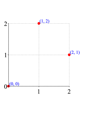
(a) Interpolation points

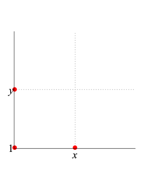
(b) Quotient ring basis

Figure 1: Lagrange interpolation

By Algorithm 2, we get

$$Q=\{1,y,x\},$$

$$G=\{y^{2},xy,x^{2}\},$$

$$\{P_{1},P_{2},P_{3}\} =\{\lambda_{G\cup Q}(e^{(0,0){\bf X}}),\lambda_{G\cup Q}(e^{(1,2){\bf X}}),\lambda_{G\cup Q}(e^{(2,1){\bf X}})\}$$

$$=\{1,~{}\frac{1}{2!}(x^{2}+4xy+4y^{2})+(x+2y)+1,~{}\frac{1}{2!}(4x^{2}+4xy+y^{2})+(2x+y)+1\}.$$

We compute a “reverse” reduced team of $\{P_{1},P_{2},P_{3}\}$, we get

$$\{P_{1}^{*},P_{2}^{*},P_{3}^{*}\} =\{1,~{}(-\frac{1}{3}x^{2}+\frac{2}{3}xy+\frac{7}{6}y^{2})+y,~{}(\frac{7}{6}x^{2}+\frac{2}{3}xy-\frac{1}{3}y^{2})+x\}.$$

Finally, the reduced Gröbner basis is read from the “reverse” reduced team $\{P_{1}^{*},P_{2}^{*},P_{3}^{*}\}$ by Line 30 in Algorithm 2, we get

$$G_{1} =y^{2}-\frac{7}{3}y+\frac{2}{3}x,$$

$$G_{2} =xy-\frac{2}{3}y-\frac{2}{3}x,$$

$$G_{3} =x^{2}+\frac{2}{3}y-\frac{7}{3}x.$$

$\{G_{1},G_{2},G_{3}\}=\{y^{2}+\frac{2}{3}x-\frac{7}{3}y,xy-\frac{2}{3}x-\frac{2}{3}y,x^{2}-\frac{7}{3}x+\frac{2}{3}y\}$ is the reduced Gröbner basis for $I(\Delta)$ w.r.t. $\prec$.

For general ideal interpolation, we can convert it to single point ideal interpolation. For example, given ideal interpolation conditions

$$\Delta=\left\{\begin{array}[]{l}\delta_{\boldsymbol{\theta}_{1}}\circ{\rm span}\{P_{11}(D),P_{12}(D),\dots,P_{1s_{1}}(D)\},\\ \delta_{\boldsymbol{\theta}_{2}}\circ{\rm span}\{P_{21}(D),P_{22}(D),\dots,P_{2s_{2}}(D)\},\\ \hskip 71.13188pt\vdots\\ \delta_{\boldsymbol{\theta}_{k}}\circ{\rm span}\{P_{k1}(D),P_{k2}(D),\dots,P_{ks_{k}}(D)\},\\ \end{array}\right.$$

where distinct points $\boldsymbol{\theta_{i}}\in\mathbb{F}^{d},i=1,2,\dots,k$ and $s_{1}+s_{2}+\dots+s_{k}=n.$ By(2), we have

$$\Delta=\delta_{\boldsymbol{0}}\circ{\rm span}\{P_{1}(D),P_{2}(D),\dots,P_{n}(D)\},$$

where $P_{1}=e^{\boldsymbol{\theta_{1}}{\bf X}}P_{11},P_{2}=e^{\boldsymbol{\theta_{1}}{\bf X}}P_{12},\dots,P_{s_{1}}=e^{\boldsymbol{\theta_{1}}{\bf X}}P_{1s_{1}},P_{s_{1}+1}=e^{\boldsymbol{\theta_{2}}{\bf X}}P_{21},\dots,\\ P_{n}=e^{\boldsymbol{\theta_{k}}{\bf X}}P_{ks_{k}}.$

The main cost of Algorithm 2 is to calculate the rank of the matrix for obtaining the monomial basis of the quotient ring. In the case of single point ideal interpolation, if the polynomials in the interpolation conditions is a “reverse” reduced team, then we can obtain the monomial basis of the quotient ring without calculation by Theorem 6. Therefore, we get a faster algorithm for computing the reduced Gröbner basis. We have the following algorithm for single point ideal interpolation.

1:  Input: A monomial order $\prec$.

2:            The interpolation conditions

$$\Delta=\delta_{\boldsymbol{\theta}}\circ{\rm span}\{P_{1}(D),P_{2}(D),\dots,P_{n}(D)\}.$$

3:            where $\boldsymbol{\theta}\in\mathbb{F}^{d},$ $\{P_{1},P_{2},\dots,P_{n}\}$ is a “reverse” reduced team.

4:  Output: $\{G_{1},G_{2},\dots,G_{m}\}$, the reduced Gröbner basis for $I(\Delta)$.

15:  //Initialization

6:  $Q:=\{{\rm lm}(P_{1}),{\rm lm}(P_{2}),\dots,{\rm lm}(P_{n})\}$, the monomial basis of the quotient ring, by Theorem 6;

7:  ${\rm{List}}:=\{x_{i}{\rm lm}(P_{j}),\forall 1\leq i\leq d,1\leq j\leq n\}$;

8:  ${\rm{List}}:={\rm{List}}-Q$;

29:  $G:=\emptyset$;

310:  //Computing

11:  while ${\rm{List}}\neq\emptyset$ do

12:     ${\bf X}^{\boldsymbol{\alpha}}:=\rm{min}(\rm{List},\prec)$;

13:     $G:=G\cup\{{\bf X}^{\boldsymbol{\alpha}}\}$;

414:     $\rm{List}:=\rm{List}-\{{\rm{multiples~{}of~{}}}{\bf X}^{\boldsymbol{\alpha}}\}$;

515:  end while

616:  $G:=\{{\bf X}^{\boldsymbol{\alpha_{1}}},{\bf X}^{\boldsymbol{\alpha_{2}}},\dots,{\bf X}^{\boldsymbol{\alpha_{m}}}\}$, the set of the leading monomials of the reduced Gröbner basis;

717:  $P_{j}:=\lambda_{G\cup Q}(e^{\boldsymbol{\theta}{\bf X}}P_{j}),~{}1\leq j\leq n$;

18:  $\{P_{j}^{*},1\leq j\leq n\}$, a “reverse” reduced team w.r.t. $\prec$, by Algorithm 1;

819:  ${\bf X}^{\boldsymbol{\beta_{j}}}:={\rm lm}(P_{j}^{*}),~{}~{}1\leq j\leq n;$

20:  for $i=1:m$ do

21:     $G_{i}={\bf X}^{\boldsymbol{\alpha_{i}}}-\sum_{j=1}^{n}\left(\frac{(\boldsymbol{\alpha_{i}})!}{(\boldsymbol{\beta_{j}})!}\hat{P}_{j}^{*}(\boldsymbol{\alpha_{i}})\right){\bf X}^{\boldsymbol{\beta_{j}}}$;

22:  end for

23:  return  $\{G_{1},G_{2},\dots,G_{m}\}$.

Algorithm 3 The reduced Gröbner basis (Single point ideal interpolation)

6 A special example for ideal interpolation

For general ideal interpolation, we convert it to single point ideal interpolation by (2) and get the “reverse” reduced team by Algorithm 1, then we compute the reduced Gröbner basis by Algorithm 3. The amount of these calculation is almost the same as MMM algorithm. However, in some special cases, we can first compute the Gröbner basis of a single point ideal interpolation by Algorithm 3(this requires little calculation),then construct the original Gröbner basis. The scale of the problem decreases in this case, thus the computational efficiency has been improved. A relevant example is given below.

Example 10

(Ideal interpolation) Given the monomial order $\mathrm{lex}(y\prec x)$ and ideal interpolation conditions

$$\Delta=\left\{\begin{array}[]{l}\delta_{(0,0)}\circ{\rm span}\{1,D_{x},\frac{1}{2}D_{x}^{2}+D_{y}\},\\ \delta_{(1,2)}\circ{\rm span}\{1,D_{x}\}.\end{array}\right.$$

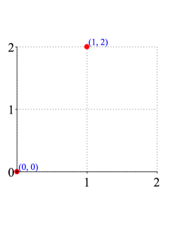
(a) Interpolation points

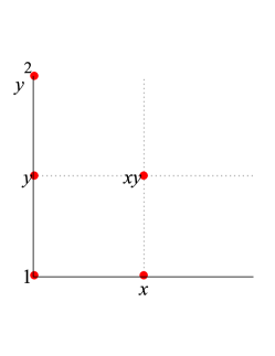
(b) Quotient ring basis

Figure 2: Ideal interpolation

We split the original problem into two subproblems $\Delta_{A}$ and $\Delta_{B}$.

$$\Delta_{A}:=\delta_{(0,0)}\circ{\rm span}\{1,D_{x},\frac{1}{2}D_{x}^{2}+D_{y}\}.$$

Since $\{1,x,\frac{1}{2}x^{2}+y\}$ is a “reverse” reduced team, $Q_{A}:=\{1,x,y\}$ is the monomial basis of the quotient ring $\mathbb{F}[{\bf X}]/I(\Delta_{A}),$ $G_{A}:=\{y^{2},xy,x^{2}\}$ is the set of the leading monomials of the reduced Gröbner basis for $I(\Delta_{A})$. By Line 21 in Algorithm 3, we get

$$G_{A1} :=y^{2},$$

$$G_{A2} :=xy,$$

$$G_{A3} :=x^{2}-y.$$

$\{G_{A1},G_{A2},G_{A3}\}=\{y^{2},xy,x^{2}-y\}$ is the reduced Gröbner basis for $I(\Delta_{A})$.

$$\Delta_{B}:=\delta_{(1,2)}\circ{\rm span}\{1,D_{x}\}.$$

With the same procedure, we can get

$$G_{B1} :=y-2,$$

$$G_{B2} :=x^{2}-2x+1.$$

$\{G_{B1},G_{B2}\}=\{y-2,x^{2}-2x+1\}$ is the reduced Gröbner basis for $I(\Delta_{B})$.

Notice that polynomials $G_{A1}=y^{2}$ and $G_{B1}=y-2$ are coprime, there exist polynomials $u=\frac{1}{4}$ ,$v=-\frac{1}{4}(y+2)$ such that

$$uG_{A1}+vG_{B1}=1.$$

Let

$$G_{1} :=G_{A1}G_{B1}=y^{3}-2y^{2},$$

$$G_{2} :=G_{A2}G_{B1}=xy^{2}-2xy,$$

$${\tilde{G}}_{3} :=(uG_{A1})G_{B2}+(vG_{B1})G_{A3}=x^{2}-\frac{1}{2}xy^{2}+\frac{1}{4}y^{3}+\frac{1}{4}y^{2}-y.$$

Since $G_{1},G_{2},{\tilde{G}}_{3}$ all lie in $I(\Delta_{A}\cup\Delta_{B})=I(\Delta)$, the linear combination ${\tilde{G}}_{3}-cG_{1}-eG_{2}$ lies in $I(\Delta)$, where $c=\frac{1}{4}$ is the coefficient of $y^{3}$ in ${\tilde{G}}_{3}$ and $e=-\frac{1}{2}$ is the coefficient of $xy^{2}$ in ${\tilde{G}}_{3}$. Let

$$G_{3}:={\tilde{G}}_{3}-cG_{1}-eG_{2}=x^{2}-xy+\frac{3}{4}y^{2}-y.$$

Notice that the leading term of $G_{i}$ in particular divides none of the nonleading terms of $G_{j}$, for $i,j\in\{1,2,3\}$, meanwhile the dimension of $\mathbb{F}[{\bf X}]/\langle G_{1},G_{2},G_{3}\rangle$ is 5. Therefore, $\{G_{1},G_{2},G_{3}\}$ is the reduced Gröbner basis for $I(\Delta)$.

${\bf References}$

References

[1]
G. Birkhoff, The algebra of multivariate interpolation, in: Constructive approaches to mathematical models, Academic Press, 1979, pp. 345–363.
[2]
B. Buchberger, Ein algorithmus zum auffinden der basiselemente des restklassenrings nach einem nulldimensionalen polynomideal, Ph.D. thesis, Innsbruck, 1965.
[3]
H. Möller, B. Buchberger, The construction of multivariate polynomials with preassigned zeros, in: J. Calmet(Ed.), Computer Algebra: EUROCAM ’82. in: Lecture Notes in Computer Science, vol. 144, Springer, Berlin, 1982. pp. 24-31.
[4]
M.G. Marinari, H.M. Möller, T. Mora, Gröbner bases of ideals defined by functionals with an application to ideals of projective points, Appl. Algebra Engrg. Comm. Comput. 4 (2) (1993) 103–145.
[5]J. Abbott, A. Bigatti, M. Kreuzer and L. Robbiano, Computing ideals of points, J. Symb. Comput.
30 (2000) 341–356.
[6]J. Farr, S. Gao, Computing Gröbner bases for vanishing ideals of finite sets of points,
Appl. Algebra Engrg. Comm. Comput. Springer LNCS 3857 (2006) 118–127.
[7]M. Lederer, The vanishing ideal of a finite set of closed points in affine space, J. Pure.
Appl. Algebra. 212 (2008) 1116–1133.
[8]
X. Jiang, S.G. Zhang, B.X. Shang, The discretization for bivariate ideal interpolation, J. Comput. Appl. Math. 308 (2016) 177–186.
[9]
D.A. Cox, J. Little, D. O’Shea, Ideal, Varieties, and Algorithms, 3rd edition, in: Undergraduate Texts in Mathematics, Springer, New York, 2007.
[10]
T. Sauer, Polynomial interpolation of minimal degree and Gröbner bases, in Gröbner Bases and Applications (Proc. of the Conf.33 Years of Gröbner Bases), Cambridge University Press, pp. 483–494.
[11]
C. de Boor, Ideal interpolation, in: Approximation Theory XI: Gatlinburg, 2004, pp. 59–91.
[12]
C. de Boor, A. Ron, On multivariate polynomial interpolation, Constr. Approx. 6(3) (1990) 287–302.
[13]
B. Shekhtman, Ideal interpolation: translations to and from algebraic geometry, Springer Vienna, 2010.