A Rule-Based Epidemiological Framework for Modelling & Simulation In the Context of the COVID-19 Pandemic

Abstract.

Motivated by chemical reaction rules, we introduce a rule-based epidemiological framework for the mathematical modelling of the COVID-19 pandemic which lies the foundations for further study of this class of models. Here we stress that we do not have a specific model in mind, but a whole collection of models which can be transformed into each other, or represent different aspects of the pandemic. Each single model is based on a mathematical formulation that we call a rule-based system. They have several advantages, for example that they can be both interpreted both stochastically and deterministically without changing the model structure. Rule-based systems should be easier to communicate to non-specialists, when compared to differential equations. Due to their combinatorial nature, the rule-based model framework we propose is ideal for systematic mathematical modelling, systematic links to statistics, data analysis in general and machine learning. Most importantly, the framework can be used inside a Bayesian model selection algorithm, which can extend unsupervised machine learning technology to gain mechanistic insight through mathematical models. We first introduce the Bayesian model selection algorithm and give an introduction to rule-based systems. We propose precursor models, all consistent with our rule-based framework and relevant for the COVID-19 pandemic. We complement the models with numerical results and, for some of them, we include analytical results such as the calculation of the number of new infections generated by an infected person during their infectious period. We conclude the article with an in depth discussion of the role of mathematical modelling through the COVID-19 pandemic.

1. Introduction

This paper is a comprehensive study, but still only an initial attempt to apply novel mathematical modelling methods to the COVID-19 pandemic. We propose a rule-based epidemiological framework and hope to use this approach to solve the still-existing prognosis problem (see Section 4.1), which is a general problem for most so-called complex systems [40]. To summarise what the reader can expect, here is a list of novelties (some of which we aim to include in the future) of our rule-based framework:

Formal Language:

We use a formal mathematical language here which we call rule-based as a foundation of our mathematical models. Rule-based models rely on an extension of reaction kinetics which was first formulated to describe chemical reactions. It has the advantage that the rules can be interpreted both stochastically and deterministically. Moreover the rule-based systems have a mathematical structure which makes them very well suited for both science communication and rigorous mathematical analysis at the same time. We can both derive stochastic processes and differential equations to describe the temporal dynamics of the pandemic and look for differences. There are several examples in Section 3 where certain qualitative properties of the models with stochastic or deterministic interpretation stay invariant under update changes. In these cases the deterministic interpretation should be favoured, as the qualitative for differential equations is very well developed. However, we also found many cases where there is a difference between the stochastic and the deterministic interpretations of the rules differ. Therefore, to avoid ambiguity, we use the stochastic case as the generic simulation approach.

Mathematical Analysis & Simulation (Scientific Computing):

We use different ways of understanding our rule-based mathematical models, and believe only in this combination we do really understand a mathematical model. A mathematical analysis, most often based on the deterministic interpretation as a differential equation, has the advantage to understand a relatively simple model more or less completely. Much in the same way a climate model can only be understood by a whole range of simulations, more complex models of a pandemic can only be understood by means of exhaustive simulation. The models in this publication are still quite modest, and we will go new ways of scientific publication by making the simulation scripts available to the public.

Model Variation:

We do not believe that in something as complex as the COVID-19 pandemic there is a single set of equations or code, like in individual based approaches, that can successfully predict the time course of the pandemic in some sense over a longer period, i.e. overcome the prognosis problem. We stick to the notion that a mathematical model should try to be minimal, i.e. minimally complex by some complexity measure [40] as long as it is sufficiently predictive. This is related to the scientific principle called Occam’s razor. As in [46], Chapter 28, we consider Occam’s razor as a natural outcome of coherent interference based on Bayesian probability. In reality this reasoning will imply the optimally predictive model will change, i.e. we will have to walk through a model space, see Section 1.5.

Data Science:

The mathematical modelling community has too long neglected the data aspect. The COVID-19 pandemic has produced a massive amount of data, see Section 4.2. The model variation and prognosis problem can only be solved together with a firm link to data science. This is a major step we like to tackle in this project in future, however this is not an easy task. We are aware of recent advances in parametrisation of mathematical models, but still believe this is largely an unsolved problem of immense importance.

1.1. Challenges Triggered By The Pandemic

The COVID-19 pandemic posed a complex set of questions to the mathematical modelling community, with nearly daily new twists and turns. This paper intends to present a systematic framework of possible models that are designed to give answers to different aspects triggered by COVID-19 pandemic observations, i.e. empirical epidemiological data. Therefore, as discussed, we are not focusing on a particular model, as is often the case in applied mathematics papers, but follow a systematic model construction approach instead. In this first publication, we do not parametrise our models with data yet, but take basic empirical facts from the data to make variable classification choices. To have a first model choice skeleton, we observe the following fundamental empirical facts about COVID-19:

Age:

From the start of observed coronavirus cases, the associated risks have strongly been age correlated [59, 57, 48].

Health Systems:

COVID-19 has put unprecedented pressure on healthcare systems worldwide. Due to the limited capacity of the national health systems or similar institutions, fatalities increased dramatically [6, 29].

Locations:

Numerous observations and simulation hint at the risk of infection being location dependent. Staying in closed rooms close to infected individual creates a higher risk of infection when compared to the same arrangement in open space [71]. We leave the investigation of location structure to future publications.

Immunity:

Immunity is now in the discussion in connection with the effectiveness of different vaccines, but it has a more general importance. For example, how long are individuals immune to new infections? Can immunity be gained in other ways, other than having had an infection or getting vaccinated? [24, 18]

Infectivity:

Infectivity is usually thought to be rather constant, only depending on outer conditions, such as location, i.e. closed narrow rooms are considered dangerous. But clearly infectivity follows a certain time course after an individual gets infected. On top of this, there is indication some individuals, perhaps depending on genetic variation, have a strong infectivity, called ’super-spreaders’ [43, 72]. However, according to our knowledge, there is no clear data source for this yet.

Behaviour:

Given the location dependency of coronavirus infections, it became clear that behavioural choices by individuals play a crucial role in pandemic spread [34].

Mobility:

Mobility was identified as a major risk factor from the beginning of the COVID-19 pandemic, as is the case for most individual to individual infection processes [34, 31, 56].

Lockdowns:

The age and location dependency of the coronavirus infection rate implied the only successful policy to combat the pandemic was to isolate vulnerable parts of society, and close places where people would get crowded together. A general decrease of mobility would also decrease risk of infections [42].

Testing:

Observed time series report tested individuals. Testing is the only way to know how much infection is out there. There is then a fundamental difference between the intrinsic dynamics of total infected individuals, and how many of these individuals we know they are really infected (or not) because they are counted and reported through testing. From a modelling perspective, this requires to include new dynamic variables or sub-types to follow the time evolution of how many individuals tested positive (or negative), and for how long a test is still reliable [52].

Vaccination:

The rapid development of vaccines gave for the first time rise to the hope that a sufficiently large percentage of populations could be immunised safely to stop the spread of the disease (herd immunity) [49, 68].

Mutations:

These are extremely important at the moment of disease emergence [13], but also the latest twist of the COVID-19 pandemic was the rapid emergence of new mutations of the virus, with some variants observed to be more infectious, and deadlier [68].

All of these items in the discussion above can only be incorporated in mathematical models after a scientific classification. Using these models the future of pandemics can be investigated, including the likelihood of major new outbreaks. The likeliness of viruses like the coronavirus crossing from animals like bats to humans is largely related to habitat and whole ecosystem destruction [30]. Is it possible to achieve herd immunity? How will herd immunity be influenced by future mutations with different infectivities? Will COVID-19 be staying forever somewhere in the world, or will we be able to eradicate it with our policy measures, and vaccination programmes [5]?

In this paper we only consider discrete classifications, see Section 1.2. After the classification the resulting types will become variables in the mathematical model. However, becoming a variable is not the only possibility to project a dependency of above concepts into a mathematical model. We will introduce rates, a fundamental concept of any dynamic, time-dependent model, and we will also use types which results in a functional dependency of rates at which events occur, such as infections, on the system state.

1.2. Classification as Structural Model Basis, Relation to Statistics

To understand our framework model approach, we must first discuss classifications, where objects are grouped into types. Following this idea, we arrive at a simple modelling question: what are the best types or classes which when used to group human individuals serving as basic objects of a mathematical model, can successfully establish a predictive model of the COVID-19 pandemic on the basis of these group interactions? The grouping of individuals we call a type, because all individuals of the group must have a common property, i.e. a type.

We would like to emphasize that it is the type that is the basic entity that connects our mathematical model to empirical data. In this context the type can be interpreted as a random variable, and the grouping of individuals according to types corresponds to random experiments. Sometimes the random experiment is easy to perform. For example, if we consider a certain population and choose age classes as types, we can simply hand out questionnaires. However, if our type is something like ‘immunity’, elaborate lab work is needed which very likely can only be measured in random samples, i.e. sub-populations.

The most important type of an individual in this context is the characterisation that an individual is ‘infected’, establishing the type $I$ as an example. More general, any epidemiological model considers interacting populations of finite-structured types of individuals which we can count inside some system boundaries, like a national or regional territory. Let $\mathcal{O}$ be the set of basic objects, here human individuals of a larger population. The individuals form the system components at the micro-level. In principle, we would need to let $\mathcal{O}$ to be parametrised by time, because we could allow the set to change when objects either enter or leave the system. But in this description of the pandemic, we assume the population size is fixed, therefore no individuals are allowed to ‘enter’ or ‘leave’. This means, if we introduce a type $D$ for ‘dead’ later on, we still count individuals of this type to be part of the population. The single layer classification of an $SIR$-model is shown in Figure 1.

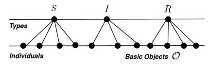
Figure 1. The object set for humans based epidemiology are usually individuals. Here, we have three types in the classical classification of human individuals, susceptible ($S$), infected ($I$) and recovered ($R$) individuals. This will be the basic classification of all models discussed, with additional classifications on top of this structure. An edge from individuals to the types, here disease states, indicates the individual are of this type.

The types are also interpreted as a scientific classification of individuals. For each classification we require that an individual is exactly of one type. However, there are possibly many different relevant classifications of individuals, such as age, or disease state etc., and these can exist in parallel. In addition, individuals can be of a certain immunity type, and they can have a certain infectivity, also a type. Let $\mathcal{T}=\{T_{1},\ldots,T_{s}\}$, $s\in\mathbb{N}$, denote the set of all possible types or individual characteristics, $s$ different types in total. It follows that we have created a hypergraph $H=H(\mathcal{O},\mathcal{T})$, i.e. the types form a set of hyperlinks, which are non-overlapping. In Section 1.4 we discuss how certain types, like age or location, are either internal or external states of an individual, and have very likely so-called sub-types. The best example is age, where the number of chosen age classes form the sub-types of the age type, i.e. the classification by age. The state of the system is given by the number of basic objects of some type, here number of human individuals that have a type at some time $t$. We use the notation that the number of these individuals of type $T_{i}$ is given by $n_{i}(t)\in\mathbb{N}_{0}$ for all $i=1,\ldots,s$.

Of course, it is possible that there is more than one system compartment in which objects can reside. In this case the types are indexed by compartment, making them compartmental sub-types. An obvious generalisation of the situation discussed here are multiple compartments, and such models will have to incorporate movement between compartments. Multi-compartment models can be used to consider geographical models of the epidemic. We leave this for future publications.

1.3. Rules

As a next step we introduce rules (or reaction channels). Let $\mathcal{R}=\{R_{1},\ldots,R_{r}\}$, $r\in\mathbb{N}$, be the finite set of rules constituting the epidemiological system. Each rule $R_{j}$ with $j=1,\ldots,r$, takes the form

$$\sum_{i=1}^{s}\alpha_{ij}T_{i}\xrightarrow{k_{j}}\sum_{i=1}^{s}\beta_{ij}T_{i},$$ (1.1)

where $k_{j}$ denotes the rate constant of rule (reaction) $R_{j}$. The sums have to be understood as so-called formal sums (as usual in reaction systems). The coefficients $\alpha_{ij}\in\mathbb{N}_{0}$ are the stoichiometric coefficients of types $T_{i}$, $1\leq i\leq s$, of the source side, and $\beta_{ij}\in\mathbb{N}_{0}$ are the stoichiometric coefficients of types $T_{i}$ of the target side of transition or reaction $R_{j}$. These stoichiometric coefficients describe changes of individual numbers due to events, such as an infection. Note that either all stoichiometric coefficients on the source side, or all stoichiometric coefficients on the target side are allowed to be zero. In this case, the formal sum is replaced by the empty set $\emptyset$.

Note that also rules are subject to confirmation by empirical data. In this case the random variable is the rule itself, and the random experiment consists of observing such a transition in the population. For example, it has never been observed that more than one infected person is needed to infect a susceptible person in the COVID-19 pandemic, therefore the stoichiometric coefficients are also observables, i.e. random variables linked to experiments.

1.3.1. Global Information

Rules are generalisations of reactions as used in so-called reaction kinetics. In epidemiology, but also other areas of science, there is a need to additionally introduce global information into the system description. The idea is that individuals know, for example from the daily news, how many infected people there are in their area, and possibly change their behaviour accordingly. Note that in chemical reaction systems, such global information is completely missing, the atoms or molecules follow only local information, i.e. they experience bumping into each other, but they do not know anything about the reaction partners before a reaction event.

We assume that the global information is collected from the type set $\mathcal{T}=\{T_{1},\ldots,T_{s}\}$, $s\in\mathbb{N}$. In this context $\mathcal{T}$ will be referred to as local types. We introduce the global information operator $\Delta$ and a global information type set, or short global types, given by $\mathcal{G}=\{G_{1},\ldots,G_{g}\}$, $g\in\mathbb{N}$. Now let

$$\Delta\colon\mathcal{T}\to\mathcal{G}.$$

Therefore, $\Delta$ takes information from the types of the model, and maps it to global information which can be made known to the system. For example, in an age-structured model, let $\mathcal{T}_{I}=\{I_{1},I_{2},\ldots,I_{n}\}$ denote the types of infected individuals inside $n$-different age classes. Let $\mathcal{G}=\{G_{I}\}$ be a one-dimensional global information type set, here interpreted as all infected individuals in the system. Then $\Delta$ is given implicitly by the formal sum

$$G_{I}:=\sum_{i=1}^{n}I_{i}.$$

In general we assume

$$G_{i}:=F_{i}(\mathcal{T}),\;\;\;i=1,\ldots,g,$$

with $F_{i}$ some function mapping $s$ many types to one type. When we introduce a state $n_{i}(t)\in\mathbb{N}_{0}$ of type $T_{i}$ at system time $t\geq 0$ for $i=1,\ldots,s$, see Section 2.1.1, then global types will at the same time have derived numerical values.

1.4. Sub-Classifications, Internal and External Individual States

We consider now the case where we need to further differentiate types into sub-types, which we often also interpret as ‘internal states’ of individuals. The best example in our current context are age classes, but in fact already the $S$-$I$-$R$ classification can be interpreted as sub-types of a general disease state. Sub-types therefore are a very important modelling idea for infectious diseases. Because types can now exist of different sub-types, we need to introduce their frequency distribution. Define $l_{i}\in\mathbb{N}$ as the number of sub-types of type $i$ for $1\leq i\leq s$. Let $\mu_{ij}^{\alpha}$ denote the frequency of the sub-type $\alpha$, $1\leq\alpha\leq l_{i}$, needed for the source terms in rule $R_{j}$, called the source frequency. We have

$$\mu_{ij}^{\alpha}=\frac{n_{ij}^{s,\alpha}}{m^{s}_{ij}},$$

where $n_{ij}^{s,\alpha}\in\mathbb{N}$ is the number of objects (individuals) of type $i$ and sub-type $\alpha$ needed for the source terms in rule $R_{j}$, and $m^{s}_{ij}:=\sum_{\alpha=1}^{l_{i}}n_{ij}^{s,\alpha}$ is the total number of objects of type $T_{i}$ needed for reaction $R_{j}$. The symbol $s$ denotes ‘source’. Clearly, we have

$$\sum_{\alpha=1}^{l_{i}}\mu_{ij}^{\alpha}=1\;\;$$ (1.2)

for all types $i=1,\ldots,s$ and all reactions $R_{j}$ for $j=1,\ldots,r$. Similarly, let $\nu_{ij}^{\alpha}$ denote the frequency of the sub-type $\alpha$, $1\leq\alpha\leq l_{i}$ after rule $j$ has been triggered, called the target frequency. We have

$$\nu_{ij}^{\alpha}=\frac{n_{ij}^{t,\alpha}}{m^{t}_{ij}},$$

where $n_{ij}^{t,\alpha}\in\mathbb{N}$ is the number of objects (individuals) of type $i$ of sub-type $\alpha$ as result of the event described by rule $R_{j}$, and $m^{t}_{ij}:=\sum_{\alpha=1}^{l_{i}}n_{ij}^{t,\alpha}$. Here the symbol $t$ denotes ‘target’. Again we have

$$\sum_{\alpha=1}^{l_{i}}\nu_{ij}^{\alpha}=1$$ (1.3)

for all types $i=1,\ldots,s$ and all reactions $R_{j}$ for $j=1,\ldots,r$. The constants $\mu_{ij}^{\alpha},\nu_{ij}^{\alpha}\in\mathbb{Q}$ specify the frequency of individuals that are necessary for each rule to be realised. They are therefore the frequency analogues of stoichiometric coefficients. Finally we can now write every possible event or rule (or reaction) $R_{j}$ in the more general form

$$\sum_{i=1}^{s}\gamma_{ij}\sum_{\alpha=1}^{l_{i}}\mu_{ij}^{\alpha}T^{\alpha}_{i}\xrightarrow{k_{j}}\sum_{i=1}^{s}\delta_{ij}\sum_{\alpha=1}^{l_{i}}\nu_{ij}^{\alpha}T^{\alpha}_{i},$$ (1.4)

for $j=1,...,r$, where the sums have to be understood again as formal sums. The coefficients $\gamma_{ij}\in\mathbb{N}$ are the stoichiometric coefficients of types $T_{i}$, $1\leq i\leq s$, of the source side, and $\delta_{ij}\in\mathbb{N}$ are the stoichiometric coefficients of types $T_{i}$ of the target side of rule $R_{j}$ with rate constant $k_{j}$. These stoichiometric coefficients describe changes of object numbers, independent of the sub-type of an object of any type. Note that if all types have just a single state or configuration, then the scheme is equivalent to a traditional reaction scheme (1.1) by construction. The generalised scheme (1.4) is useful, for example, we can use it to establish a varying number of discrete age classes in a single rule.

1.5. Towards an Epidemiological Modelling Framework

We are now ready to establish our modelling framework, which by construction will become a discrete and finite model space. As we will argue, this is important as we later like to apply machine learning technology. A discrete model space will be more easily searchable by automated methods, comparing their predictions with data. However, there needs to be a fundamental discussion on whether we can construct such a discrete and finite model space which must incorporate models that are predictive, otherwise the construction would be useless. Moreover we must fix an interpretation of the identity of a model, i.e. answer the question when two models are different? All these questions will occupy us in future publications. We summarize our findings in the following list:

Structural (Mathematical) Ontology:

When are two models different? We believe this depends on the kind of question being asked. The two possibilities are: (i) the model structure only decides whether two models are different, independent of any empirical association, or (ii) two models become different if they are allowed to have identical structure, but different empirical interpretation. Following (i), we can mathematically investigate a model, for example the qualitative behaviour, which will be the same independent of any empirical association. This is the usual mathematical approach. For example, considering simplicial complexes in algebraic geometry, the same simplex can occur several times in a complex, see [35], page 70. Indeed, if we construct models, for example on basis of rule-based systems, we might like to define algebraic operations on models, adding or subtracting types and rules in order to derive new models. This will become similar to the concept of a $q$-chain, the starting point of the homology of simplicial complexes, just with replacing $q$-simplices with models having a certain number of types and rules. See [35], page 179. Such a concept we refer to as structural ontology.

Empirical Ontology:

When are two models different, based on empirical data? It is best to understand this question by an example. Consider the model

$$T_{1}+T_{2} \xrightarrow{\alpha} 2T_{2}$$ (1.5)

$$T_{2} \xrightarrow{\beta} T_{3}$$

with $3$ types and $2$ rules. If we set $(T_{1},T_{2},T_{3})=(S,I,R)$, then we recover the simplest infection model (3.1). Setting the types in this way makes a connection to empirical data, as from now onwards we can make measurements in a given population, for example to check whether this model is predictive. By setting $T_{1}$ to a certain well-defined opinion, $T_{2}$ to another well-defined opinion, and $T_{3}$ to, say, no opinion about the subject at all, i.e. being indifferent, this makes (1.5) an opinion formation model. As this model would be evaluated according to very different data, it would make the two models empirically different. We call this interpretation empirical ontology.

1.5.1. Model Approximation

It is clear that a discrete and finite model space will be a challenge for many applied mathematicians, especially those having grown up in the continuum world formulated by integral and partial differential equations. It is best to compare and discuss our approach with the Kermack-McKendrick epidemic model from $1927$ [37], which is rightfully seen as the standard continuum model in epidemiology. Here we follow narrowly the presentation in [12]. Assume the population is closed, i.e. no individuals either enter or leave the area under consideration. The starting point for bookkeeping in the Kermack-McKendrick model are the following two quantities:

$$\begin{split}F(t):\;\;&\text{force of infection at time}\;\;t,\;\;\\ S(t):\;\;&\text{density (number per unit area) of susceptibles at time}\;\;t.\;\;\\ \end{split}$$ (1.6)

Here the force of infection is, by definition, the probability per unit of time that a susceptible becomes infected. The key necessary assumption of the continuum approach is that numbers of individuals in any disease state are large enough to warrant a deterministic description. Under this assumption, we then have

$$\text{incidence}=F(t)S(t),$$

where ’incidence’ is defined as the number of new cases per unit of time and area. If the variable $S$ only changes due to transmission of infection, i.e.,

$$\frac{d}{dt}S(t)=-\text{incidence},$$

valid under the assumption the infection leads to permanent immunity, therefore no new susceptibles can reappear. A key modelling ingredient next needed is

$$A(\tau):=$$ expected contribution to the force of infection by an individual

$$\text{that was itself infected $\tau$ units of time ago}.$$

The function $A$ from a modelling point of view has two ingredients, (i) a contact intensity, and (ii) infectiousness. The latter is the probability of transmission of the disease, given a contact with a susceptible. Clearly by interpretation we need to assume $A(\tau)\geq 0$. Moreover, we assume that

$$A:[0,\infty)\to[0,\infty)$$

is integrable. Typical explicit algebraic expressions for $A(\tau)$ are

$$A(\tau):=\beta e^{-\alpha\tau},$$ (1.7)

$$A(\tau):=\beta\frac{\gamma}{\gamma-\alpha}(e^{-\alpha\tau}-e^{-\gamma\tau}).$$ (1.8)

Note that $R_{0}$, the basic reproduction ratio defined as the expected number of secondary cases caused by a primary case introduced in a population with susceptible density $S(-\infty)$, is given by

$$R_{0}:=S(-\infty)\int_{0}^{\infty}A(\tau)d\tau,$$

compare with Section 3.1.4. The constitutive equation

$$F(t)=\int_{0}^{\infty}F(t-\tau)S(t-\tau)A(\tau)d\tau$$ (1.9)

now tells us how the current force of infection depends on past incidence. By integrating

$$\frac{d}{dt}S(t)=-F(t)S(t)$$

we obtain

$$S(t)=S(-\infty)\;e^{-\int_{-\infty}^{t}F(\sigma)d\sigma}.$$ (1.10)

If we substitute (1.9) into (1.10), we obtain a nonlinear scalar renewal equation for the unknown $F$. Now we introduce the cumulative force of infection

$$y(t):=\int_{-\infty}^{t}F(\sigma)d\sigma.$$

Using essentially (1.9) and (1.10) again, we can derive a scalar nonlinear renewal equation of convolution type for $y$:

$$y(t)=\int_{0}^{\infty}(1-e^{-y(t-\tau)})S(-\infty)A(\tau)d\tau.$$ (1.11)

The limit $y(\infty)=\lim_{t\to\infty}y(t)$ exists and satisfies the equation

$$y(\infty)=R_{0}(1-e^{-y(\infty)}).$$

The latter equation has a strictly positive solution $y(\infty)$ if $R_{0}>1$, which corresponds to an epidemic outbreak of final size. For comparison with our approach, one has to note that by using kernels of matrix exponentials like (1.7) and (1.8), delay equations correspond to systems of ordinary differential equations (ODE), which represent a finite closed moment expansion. This has been named ‘Linear Chain Trickery’, see [45]. The reader can check that assumption (1.7) leads to an SIR ODE model, and assumption (1.8) leads to an SEIR ODE model, compare with Section 3.1. The first and most significant difference between the continuum approach discussed here, and our discrete individual approach based on stochastic processes, is that we do not assume from start that infinitely many individuals are present in every type. This means we can also cover small number events, which are important in cases where some types are represented by a very low number of individuals. Note that this can be important at the start of an epidemic, but also during a pandemic, when individual numbers of one ore more types approach $0$. However, there is of course the question whether the renewal equation (1.11) is more general than our approach. In the end, it is well-defined for non-exponential choices of $A(\tau)$, giving enormous flexibility to the Kermack-McKendrik model. We seem not to have this flexibility in our framework, because it is based generically on exponential waiting times for events to happen. But note that we can use a generalised Gillespie algorithm to create the respective stochastic processes, and this can cover any waiting time distribution, see Section 2.1.2. However, it is an open mathematical question whether a Gillespie-based stochastic process using arbitrary waiting time distributions, together with a continuum limit (where individual numbers become infinite), can approximate the Kermack-McKendrick model with arbitrarily given kernels $A(\tau)$.

1.5.2. Model Support Space

Rule-based systems are characterised by the set of types, the set of rules, and the set of parameters. As a fundamental assumption we suppose that all these sets are finite. As before, assume all possible epidemiological framework models have at most the set $\mathcal{T}=\{T_{1},\ldots,T_{s}\}$, $s\in\mathbb{N}$, as the maximal set of types, and $\mathcal{R}=\{R_{1},\ldots,R_{r}\}$, $r\in\mathbb{N}$, as the maximal set of rules, and $\Theta=\{\vartheta_{1},\ldots,\vartheta_{t}\}$, $t\in\mathbb{N}$. The finiteness of the number of rules, types and parameters is a strong, but reasonable assumption, especially if existing classical models can be approximated sufficiently well, see Section 1.5.1. Depending on the choice of $r,s\in\mathbb{N}$, it is possible to consider a large number of different models where each model consists of subsets of types $\mathcal{T}$ and rules $\mathcal{R}$ at their disposal. In addition, we require that the state space associated with the model space is discrete, therefore we will need to define a stochastic process describing changes of numbers in each type. The idea with changing types and rules in an empirical setting is of course that different mechanisms will not be constant over arbitrary time intervals, therefore the model structure will need to change, given the data. A more detailed discussion is given in Section 4.1. The following two conditions seem appropriate:

1. All states of type $T_{i}$ satisfy $n_{i}(t)\in\mathbb{N}_{0}$ for all $i=1,\ldots,s$, implying that the state space is fixed maximally to $(\mathbb{N}^{+}_{0})^{s}$.

2. The update interpretation of the rules is fixed. We use continuous-time Markov chains (see Section 2.1.1), with transition probabilities computed by the Gillespie algorithm (see Section 2.1.2).

On the basis of these assumptions we can indeed assemble every possible model within the framework. A model will be represented by a subset of the model support space $\mathcal{S}:=\mathcal{T}\times\mathcal{R}\times\Theta$, see Figure 2, showing a projection to $\mathcal{T}\times\mathcal{R}$ space only. Of course we can exchange some of our basic assumptions, for example assuming a deterministic interpretation by mass-action kinetics. This would just change the model space, not the number of possible models.

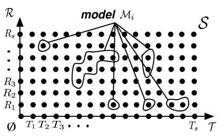
Figure 2. The model support space $\mathcal{S}$. Only types and rules are used to characterize a model.

1.5.3. The Model Space

All models in the epidemiological framework are represented by the power set of the model support space $\mathcal{S}$, i.e. the set of all subsets of $\mathcal{S}$. For constructing the model space $\mathcal{M}$, we consider the power sets of $\mathcal{T}$, $\mathcal{R}$ and $\Theta$, denoted by $\mathcal{P}^{\mathcal{T}}$, $\mathcal{P}^{\mathcal{R}}$, and $\mathcal{P}^{\Theta}$ respectively. We set $\mathcal{M}:=\mathcal{P}^{\mathcal{T}}\times\mathcal{P}^{\mathcal{R}}\times\mathcal{P}^{\Theta}$ with $M:=|\mathcal{M}|=|\mathcal{P}^{\mathcal{T}}||\mathcal{P}^{\mathcal{R}}||\mathcal{P}^{\Theta}|=2^{r+s+t}$. Here $|\cdot|$ denotes the number of elements in a finite set. Finally, we index all models (points) in $\mathcal{M}$ by the natural numbers $1,\ldots,2^{r+s+t}$. The projected model space is illustrated in Figure 3.

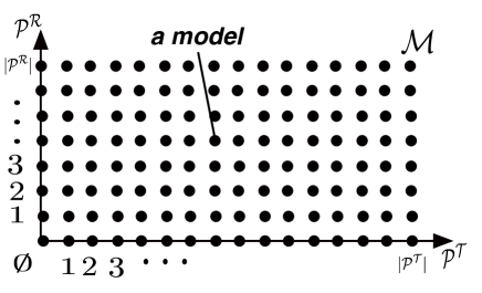
Figure 3. Each point in $\mathcal{M}$ represents a possible model of the epidemiological framework.

We can introduce an ordering and distance measure in the model space $\mathcal{M}$. Let $\vartheta_{i}$ be the vector of real-valued parameters associated to model $\mathcal{M}_{i}$, having length $|\vartheta_{i}|$, i.e. $\vartheta_{i}=(\vartheta_{i,1},\ldots,\vartheta_{i,|\vartheta_{i}|})\subset\Theta$. The ordering should be based on the structural ontology of the model, not directly on empirical ontology, i.e. two models with exactly the same types, rules and parameters, independent of interpretation, should in this sense be identical, see Section 1.5. We can interpret this as models having identical mathematical structure, with the same kind of feedback loops present in the system. We therefore classify the model by types, rules and parameters being used in its structure, i.e. a model $\mathcal{M}_{i}$ has mathematical structure $\mathcal{M}_{i}(\mathcal{T}_{i},\mathcal{R}_{i},\vartheta_{i})$. To each model we attach a complexity measure $\mathrm{C}(\mathcal{M}_{i}):=|\mathcal{T}_{i}|+|\mathcal{R}_{i}|+|\vartheta_{i}|$. Given two models $\mathcal{M}_{i}(\mathcal{T}_{i},\mathcal{R}_{i},\vartheta_{i})$ and $\mathcal{M}_{j}(\mathcal{T}_{j},\mathcal{R}_{j},\vartheta_{j})$, a distance measure is given by

$$\operatorname{dist}(\mathcal{M}_{i},\mathcal{M}_{j}):=|(\mathcal{T}_{i}\cup\mathcal{T}_{j})\setminus(\mathcal{T}_{i}\cap\mathcal{T}_{j})|+|(\mathcal{R}_{i}\cup\mathcal{R}_{j})\setminus(\mathcal{R}_{i}\cap\mathcal{R}_{j})|+|(\vartheta_{i}\cup\vartheta_{j})\setminus(\vartheta_{i}\cap\vartheta_{j})|.$$ (1.12)

The distance measures how many types and rules are mutually missing from each other, and would need to be introduced in order to make the models more similar. Next we define an order relation between $\mathcal{M}_{i}(\mathcal{T}_{i},\mathcal{R}_{i},\vartheta_{i})$ and $\mathcal{M}_{j}(\mathcal{T}_{j},\mathcal{R}_{j},\vartheta_{j})$, by

$$\mathcal{M}_{i}>\mathcal{M}_{j}\Leftrightarrow\mathrm{C}(\mathcal{M}_{i})>\mathrm{C}(\mathcal{M}_{j}).$$

The obvious interpretation is that a model is larger if it has both more types, rules and parameters. We also say model $\mathcal{M}_{i}$ is more complex than model $\mathcal{M}_{j}$ in case $\mathcal{M}_{i}>\mathcal{M}_{j}$.

1.6. Data And Bayesian Model Selection

The basic framework models introduced in Section 3 form a model pool, where each possible model has to be compared with available data to test its predictive power. This opens the question of model selection. Here we propose to use a Bayesian Ockham’s razor and closely follow [46], Chapter 28. To start the discussion, we enumerate all possible framework models in a finite model list, as introduced in the previous section 1.5.3. Let

$$\mathcal{M}:=\{\mathcal{M}_{1},\ldots,\mathcal{M}_{M}\},$$

be that list. Each model $\mathcal{M}_{i}$ has a list of parameters $\vartheta_{i}$. In the case of classical reaction kinetics, each rule $R_{j}$ has just one parameter $k_{j}\in\mathbb{R}^{+},\;1\leq j\leq r$, the reaction constant, see equation (1.4). Therefore in such rule-based models, the number of parameters is equal to the number of rules. But in typical epidemiological models, the situation is more complex. We can now transform one model of the framework into another by either changing the set of types, changing the set of rules, or introducing different parameters, see section 1.5.2.

1.6.1. Model parameter fitting.

To compare a specific model with given data, we have to fit the model parameters to the given data in a first step. Therefore, at a first level of inference we assume some model $\mathcal{M}_{i}$ is true, which means it is a correct description of the real-world situation. Using Bayesian reasoning, i.e. Bayes’ theorem, we have

$$P(\vartheta_{i}|D,\mathcal{M}_{i})=\frac{P(D|\vartheta_{i},\mathcal{M}_{i})P(\vartheta_{i}|\mathcal{M}_{i})}{P(D|\mathcal{M}_{i})},$$ (1.13)

where $D$ denotes given data. Here $P(\vartheta_{i}|D,\mathcal{M}_{i})$ is the posterior, i.e. the probability of having the correct parameter set $\vartheta_{i}$, given the empirical data $D$ and the ‘true’ model $\mathcal{M}_{i}$. Next $P(D|\vartheta_{i},\mathcal{M}_{i})$ is the likelihood of having measured the correct data, assuming $\vartheta_{i}$ and $\mathcal{M}_{i}$ are known and chosen correctly. The term $P(\vartheta_{i}|\mathcal{M}_{i})$ is called the prior, it is incorporating our belief that model $\mathcal{M}_{i}$ is correct before the parameter estimation, i.e. without knowing the data. Finally $P(D|\mathcal{M}_{i})$ is the evidence that the data are correct, given the model $\mathcal{M}_{i}$. Inside parameter estimation, it can be interpreted as a normalising constant, and therefore is commonly ignored during this level of inference. Parameter estimation is done using an iterative numerical algorithm, for example steepest gradient descent, or a method based on Newton iteration. The iteration consists of making the previously computed posterior the new likelihood in Bayes formula (1.13).

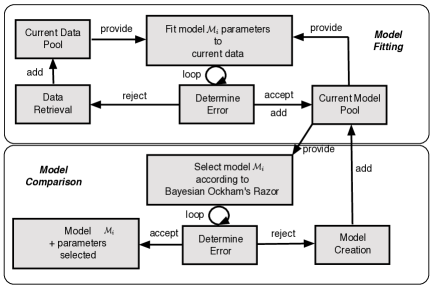
Figure 4. A diagram visualising the steps towards model selection. The upper box illustrates model parameter fitting, see Section 1.6.1, the lower box model selection, or comparison, Section 1.6.2. The two problems are connected.

In Figure 4 parameter fitting is represented by the upper box of the diagram, where the loop indicates that models have to be fitted and the error for the new parameter values have to be determined. In the ideal case the posterior has a unique maximum to which the iterative method converges. We denote the values of this best-fit parameter set by $\hat{\vartheta}_{i}$. The goal is to represent the posterior distribution by the value $\hat{\vartheta}_{i}$, together with error bars or confidence intervals around $\hat{\vartheta}_{i}$. Error bars can be obtained from the curvature of the posterior by evaluating the Hessian at $\hat{\vartheta}_{i}$, therefore let

$$A:=-\nabla^{2}\ln P(\vartheta_{i}|D,\mathcal{M}_{i})|_{\hat{\vartheta}_{i}}.$$

Now performing a Taylor expansion of the log posterior at $\Delta\vartheta_{i}:=p_{i}-\hat{\vartheta}_{i}$ gives

$$P(\vartheta_{i}|D,\mathcal{M}_{i})\simeq P(\hat{\vartheta}_{i}|D,\mathcal{M}_{i})\exp(-\frac{1}{2}p_{i}^{T}A\;\Delta\vartheta_{i}),$$ (1.14)

read the posterior is proportional to the right hand side of equation (1.14). This means the posterior distribution can be interpreted as being locally approximated as a Gaussian with covariance matrix $A^{-1}$. The covariance matrix $A^{-1}$ can be interpreted as error bars, giving the parameter estimation problem a proper statistical setting. Maximisation of the posterior probability is only useful if (1.14) gives indeed a good summary of the distribution. How the epidemiological framework models behave in this respect is still subject to investigation. However note that determining the likelihood is often costly or even impossible, especially when considering real world data like epidemiological time series. To overcome this in the Bayesian setting, simulation based so called Approximate Bayesian Computation (ABC) methods are used. This is one of the reasons why we focus on simulations in this paper. For underlying algorithms see also [1]. The general problem of underfitting and overfitting of mathematical problems related to the number of model parameters is discussed in [14].

1.6.2. Model selection.

The general problem of model selection can be expressed as the information loss when approximating the ’truth’ or ’reality’, assumed to be a mathematical model, with another mathematical model. The models $\mathcal{M}_{i}$ themselves, including reality $\mathcal{M}_{\text{R}}$, are given by probability distributions on the reality space $\Omega$ (assumed to be a set), containing everything that can possibly be empirically sampled. For $x\in\Omega$ define

$$I(\mathcal{M}_{\text{R}},\mathcal{M}_{i}):=\int_{\Omega}\mathcal{M}_{\text{R}}(x)\log\left(\frac{\mathcal{M}_{\text{R}}(x)}{\mathcal{M}_{i}(x|\mathcal{T}_{i},\mathcal{R}_{i},\vartheta_{i})}\right)\;dx.$$ (1.15)

This is the so-called Kullback-Leibler distance between probability distributions, see [14], p. 51. The log in the formula is the natural logarithm. Then, as claimed, (1.15) describes the loss of information when reality is approximated with one of our mathematical models from our framework model space, Section 1.5.3. The fundamental problem of model selection is to minimise $I(\mathcal{M}_{\text{R}},\mathcal{M}_{i})$ within the given framework. Equation (1.15) is also the starting point for various reality approximations, like the Akaike information criterium (AIC), see [14].

Of course we do not know reality, with the only possibility left to know it better by doing more and more empirical measurements, i.e. increasing $D$ in our notation. The usual way to avoid a direct comparison with the real world is to look at comparable model performance relative to given data: going back to the previous Section 1.6.1, we could as a first step do parameter fitting for any given empirical data set $D$ for each of the models $\mathcal{M}=\{\mathcal{M}_{1},\ldots,\mathcal{M}_{M}\}$ simultaneously. However, this is of course generally computationally expensive, or even impossible. The most promising method is a search in model space, using the posterior probability that a given model $\mathcal{M}_{i}$ is correct, satisfying

$$P(\mathcal{M}_{i}|D)\;\propto\;P(D|\mathcal{M}_{i})P(\mathcal{M}_{i}),$$ (1.16)

up to a proportionality constant

$$P(D):=\sum_{i=1}^{M}P(D|\mathcal{M}_{i})P(\mathcal{M}_{i}),$$

which does not change any model ranking. Note that we will not compute $P(D)$, as this constant would need information over the whole model space, contradicting any more sensible search strategy. The search strategy itself could be based on machine learning or similar technology. It does involve model generation, where types, rules and parameters are systematically varied. The method can also incorporate expert insight, like ’there was a behavioural change in the population’. Model selection or comparison is a never ending story as more and more data can always be collected. This iterative open loop is also illustrated in Figure 4, as the second loop between the current model and error boxes in the lower part of the diagram. The term $P(\mathcal{M}_{i})$ is a prior over model space, which expresses how plausible a model is before the empirical data $D$ arrive. We note that the epidemiological framework models differ in their type set, therefore their underlying classification and $P(\mathcal{M}_{i})$ can differ, for example, if there is a priori knowledge the data will be structured according to the same or similar type set. If the data is age-structured, as is often the case in the COVID-19 pandemic, we would surely give a higher probability $P(\mathcal{M}_{i})$ to models which are also age-structured. But of course eventually, according to (1.16), we need to evaluate the evidence $P(D|\mathcal{M}_{i})$. Only then can we start a proper model comparison. This means that the evidence, which is useless in the process of parameter fitting, see (1.13), plays a crucial role. The evidence embodies Ockham’s razor, a fundamental scientific concept favouring less complex models. We need $P(D|\mathcal{M}_{i})$ to be set up such that more complex models, mostly those with more parameters, will have less evidence. Ockham’s razor then requires

$$P(D|\mathcal{M}_{i})>P(D|\mathcal{M}_{j})\;\;\text{if and only if}\;\;\mathcal{M}_{i}<\mathcal{M}_{j}.$$

However, as we have only a partial order in model space, the model comparison problem remains challenging. We will devote a number of publications in relation to our framework approach to this topic.

2. Modelling Framework

We are now able to present our epidemiological framework in more detail. We first look briefly at the connection to structural (static) modelling.

2.1. Introducing Dynamics

2.1.1. Continuous-Time Markov Chains Including Global Information

In this section, we formulate reactions (1.1) as a continuous-time Markov chain. We regard the size/number $n_{i}(t)\in\mathbb{N}$ of type $T_{i}$ at system time $t\geq 0$ for $i=1,\ldots,s$ as discrete random variables with values in $\{0,\ldots,N\}$. For defining the transition probabilities associated with the stochastic process we assume that the process is time-homogeneous (autonomous), i.e., while no event occurs, the transition probabilities remain constant, and depend only on the time between events $\Delta t$, but not on the specific time $t$. We observe the system from time $0$ up to time $T>0$. In addition, we suppose that the Markov property is satisfied, that is, the probability distribution of a future state of the stochastic process at time $t+\Delta t$ only depends on the current state at time $t$, but not on any state prior to $t$. With each type $T_{i}$ having an associated state $n_{i}(t)\in\mathbb{N}$, the global type set $\mathcal{G}=\{G_{1},\ldots,G_{g}\}$, see Section 1.3.1, get derived numerical values which are. We assume at system time $t\geq 0$ to obtain the global state vector $\vartheta(t):=(\vartheta_{1}(t),\ldots,\vartheta_{g}(t))$, with $\vartheta_{i}\in\mathbb{R}$ for $1\leq i\leq g$. Given the system is in state (or configuration) $n$, we introduce the propensities $\kappa_{j}(t^{\prime},n)$ for $j=1,\ldots,r$. Here, the propensity $\kappa_{j}(t^{\prime},n)$ of the $j$th reaction $R_{j}$ is the probability that the $j$th event/reaction occurs within an infinitesimal time interval, the last event in the entire system happened at $t^{\prime}$, and is given by

$$\kappa_{j}(t^{\prime},n)=k_{j}f_{j}(\vartheta(t^{\prime},n))\prod_{i=1}^{s}\begin{pmatrix}n_{i}\\ \alpha_{ij}\end{pmatrix},$$ (2.1)

where $\kappa_{j}(\vartheta(t^{\prime}))$ denotes the global state dependent propensities of reaction $R_{j}$, $k_{j}$ is the reaction constant, and the combinatorial factor reflects the number of ways in which reaction $R_{j}$ may happen, see (1.1). The functions $f_{j}$, $1\leq j\leq r$, are called global information functional responses. These functions modify the rule execution constants $k_{j}$ according to the state of the given global information vector $\vartheta$.

Remark 2.1

Note that the notation $\kappa_{j}(t^{\prime},n)$ suggests time-dependence, which is not the case, therefore simply writing $\kappa_{j}(n)$ is equally valid and will be adopted sometimes. The notation is just a reminder that the propensity depends on the last event that happened in the system, as then the global information available to the system is updated. Time-homogeneity and the Markov property are still valid piecewise. In more sophisticated situations however, such as externally imposed lockdowns, the time-dependency of the propensity $\kappa_{j}$ will have to be considered explicitly.

We use some standard algebraic expressions for global information functional responses $f_{j}(\vartheta)$ in case $\vartheta$ is one-dimensional and non-negative:

Simple Saturation:

$$f_{j}(\vartheta):=\frac{1}{1+\lambda_{j}\vartheta}.$$

Here $\lambda_{j}$ is an additional positive parameter. We also consider $\frac{1}{f_{j}}$ in case the functional response has to be monotonically decreasing, due to modelling purposes.

Michaelis-Menten:

$$f_{j}(\vartheta):=\frac{1}{\lambda_{j}+\vartheta}.$$

Here $\lambda_{j}$ is an additional positive parameter. Alternatively, we may consider $\frac{1}{f_{j}}$ in case the functional response is monotonically decreasing.

Exponential:

$$f_{j}(\vartheta):=\lambda_{j}e^{-\lambda_{j}\vartheta}.$$

Here $\lambda_{j}$ is an additional positive parameter. The exponential functional response gives rise to a probability measure $P_{j}$, with distribution function $F_{j}(\vartheta)=1-\lambda_{j}e^{-\lambda_{j}\vartheta}$, and is called exponential distribution. For $\varepsilon>0$, we define a loss rate $\lambda(\vartheta)$ by

$$\lambda(\vartheta):=\lim_{\varepsilon\to 0}\frac{P((\vartheta,\vartheta+\varepsilon])}{P((\vartheta,\infty))}.$$

It follows that

$$\lambda(\vartheta)=\frac{f_{j}(\vartheta)}{1-F_{j}(\vartheta))}.$$

Weibull:

$$f_{j}(\vartheta):=\lambda_{j,1}\lambda_{j,2}\vartheta^{\lambda_{j,2}-1}e^{-\lambda_{j,1}\vartheta^{\lambda_{j,2}}}.$$

Here $\lambda_{j,1},\lambda_{j,2}$ are positive parameters. Note that for $\lambda_{j,2}=1$, $f_{j}$ reduces to the exponential distribution.

If the global state vector $\vartheta(t):=(\vartheta_{1}(t),\ldots,\vartheta_{g}(t))$ has dimension $g>1$, then each of the global information functional responses is assumed to be given in a multiplicative way by $g$-many sub-functionals, each dependent on one component of $\vartheta$:

$$f_{j}(\vartheta)=f_{j,1}(\vartheta_{1})f_{j,2}(\vartheta_{2})\cdots f_{j,g}(\vartheta_{g}),$$

where each $f_{j,i}$ is given by one of the one-dimensional algebraic expressions given above. From a modelling point of view, this assumes different global information states have an independent influence on the event rate of a rule, such as an infection. An example would be avoidance and mobility. Avoidance can be modelled by a monotonically decreasing functional response, mobility as a monotonically increasing functional response. Now, based on the assumption that at most one reaction can occur within an infinitesimal time interval $\Delta t$, the transition rates for the Markov process, given that the system is in state $n$, can then be approximated as $\kappa_{j}(n)\Delta t$ for reaction $R_{j}$ to occur within time interval $\Delta t$ and $1-\sum_{j=1}^{r}\kappa_{j}(n)\Delta t$ for no reaction to occur within time interval $\Delta t$. To simulate the sample paths of the continuous-time Markov chain, one can apply the Gillespie algorithm. The simulation of many trajectories of the system allows the computation of the statistics of evolution.

2.1.2. Gillespie’s Algorithm

The most important stochastic update idea for epidemiological models is Gillespie’s Stochastic Simulation Algorithm (SSA) and its generalisation. It is the main algorithm used to study the stochastic evolution of the models presented in this paper. This evolution arises due to the interactions among types $\mathcal{T}$ and, in the language of reaction schemes, can be expressed as a reaction network. Reaction $R_{j}$ is given by Equation (1.1) for $j=1,\ldots,r$, where $k_{j}$ denotes the rate constant of reaction $R_{j}$. Interpreting a reaction as a rule, we will use the terms reaction and rule interchangeably. Each process occurs with a propensity $\kappa_{j}(n)$, defined as

$$\kappa_{j}(n):=k_{j}\,h_{j}(n),$$ (2.2)

where

$$h_{j}(n):=\prod_{i=1}^{s}\begin{pmatrix}n_{i}\\ \alpha_{ij}\end{pmatrix}.$$

Here, the combinatorial factor $h_{j}$ describes the number of ways in which reaction $R_{j}$ takes place. As in the original paper [28] by Gillespie, we make the following assumption:

Assumption 2.2

Reaction $R_{j}$ occurs within a time interval $\Delta t$ with probability $\kappa_{j}(n)\Delta t$.

For a given population with system configuration $n\in\mathbb{R}^{s}$, one can show (see [28]) that the probability density associated with the occurrence of $R_{j}$ is given by

$$\Phi_{j}(n,t)=\kappa_{j}(\vartheta(n),n)\exp\left(-\sum_{l=1}^{r}\kappa_{l}(\vartheta(n),n)\,t\right)$$ (2.3)

as a function of time $t$. The probability that reaction $R_{j}$ ever occurs is given by

$$\rho_{j}(n)=\int_{0}^{\infty}\mathop{}\!\mathrm{d}t^{\prime}\,\Phi_{j}(n,t^{\prime})=\frac{\kappa_{j}(\vartheta(n),n)}{\sum_{l=1}^{r}\kappa_{l}(\vartheta(n),n)}$$ (2.4)

for $j\in\{1,...,r\}$. The rules given by Equation (1.1) generate a stochastic process which satisfies the Markov property due to Assumption 2.2. This process is the starting point for the derivation of the master equation, describing the time evolution of the probability distribution of the system as a whole (see [25]). The probability density in (2.3) can be interpreted in terms of reaction waiting times and, in fact, instead of Assumption 2.2, we can equivalently assume that reaction $R_{j}$ occurs with an exponentially distributed reaction waiting time. In [28] Gillespie showed that the master equation can be exactly solved through the construction of realisations of the stochastic process associated to (1.1). This is achieved through the following algorithm, where $::=$ denotes replacement:

Algorithm 2.1

[Gillespie Algorithm]

0:

Initialize the starting time $t$, the system configuration $n=(n_{1},\ldots,n_{s})$ and the rate constants $k_{j}$ for $j=1,\ldots,r$.

1:

Generate two random numbers $r_{1},r_{2}$ uniformly distributed in $[0,1]$.

2:

Set $\Phi:=\sum_{l=1}^{r}\kappa_{l}(n)$ and compute $\tau:=-\frac{1}{\Phi}\ln r_{1}$.

3:

Set $t::=t+\tau$ as the time of the next rule execution.

4:

Determine the reaction $R_{i}$ which is executed at time $t$ by finding $i$ such that

$$\frac{1}{\Phi}\sum_{l=1}^{i-1}\kappa_{l}(n)<r_{2}\leq\frac{1}{\Phi}\sum_{l=1}^{i}\kappa_{l}(n).$$ (2.5)

5:

Execute rule $R_{i}$ and update the new system configuration $n$.

6:

Go to step 1 if $t<T$, otherwise stop.

The random numbers generated in Algorithm 2.1 are used for determining the index $i$ of the next rule to be triggered, and the time interval $\tau$ for reaction $R_{i}$ to occur. By the definition of $\rho_{l}(n)$ in (2.4) we have

$$\frac{1}{\Phi}\sum_{l=1}^{i}\kappa_{l}(n)=\sum_{l=1}^{i}\int_{0}^{\infty}\mathop{}\!\mathrm{d}t^{\prime}\,\Phi_{l}(n,t^{\prime})=\sum_{l=1}^{i}\rho_{l}(n)$$

in step 4 in Algorithm 2.1. We use Gillespie’s algorithm to simulate the model dynamics, based on the assumption that the processes have exponentially distributed waiting times or, equivalently, that they are all Poisson processes, like atomic or molecular mixtures of gases or liquids. In complex systems formed by types which are heterogeneous and evolve through diverse interactions that cannot be always characterised by exponentially distributed waiting times, therefore the Gillespie approach is not fully adequate. It is thus very important to have a generalisation of Gillespie’s algorithm that allows us to study systems driven by processes with different waiting time distributions and not necessarily exponentially distributed waiting times. Several generalisations exist in the literature, see [3], [27], [50] and [8] for instance, where a generalised Gillespie algorithm based on a generalised master equation in the form of an integro-differential equation [3] may be considered.

2.1.3. Kolmogorov Differential Equations and Master Equations

Based on the propensities $\kappa_{j}(n)$ in (2.1), we state the forward Kolmogorov differential equations which are also referred to as master equations and can be used to predict the future dynamics. The Kolmogorov differential equations can be regarded as an alternative way to define the continuous-time Markov chain. We denote by $p_{n}(t)$ the probability that the system is in state $n$ at time $t$. For determining the time derivative $\frac{\mathop{}\!\mathrm{d}p_{n}(t)}{\mathop{}\!\mathrm{d}t}$, all transitions resulting in state $n$ and all transitions away from state $n$ have to be considered. Under the assumption that at most one reaction can occur within an infinitesimal time interval, we consider $m^{(j)}=(m^{(j)}_{1},\ldots,m^{(j)}_{s})$ for $j=1,\ldots,r$ as the transition between states for reaction $R_{j}$ where $m^{(j)}_{i}$ denotes the difference of individuals of type $T_{i}$ before and after reaction $R_{j}$ for $i=1,\ldots,s$. If the system is in state $n-m^{(j)}$ before reaction $R_{j}$ occurs, this leads to state $n$ after reaction $R_{j}$ occurs. We formulate the Kolmogorov equations as

$$\frac{\mathop{}\!\mathrm{d}p_{n}(t)}{\mathop{}\!\mathrm{d}t}=\sum_{j=1}^{r}\left(\kappa_{j}(n-m^{(j)})p_{n-m^{(j)}}(t)-\kappa_{j}(n)p_{n}(t)\right).$$ (2.6)

Note that (2.6) can be written as a linear ordinary differential equations (ODEs) of the form

$$\frac{\mathop{}\!\mathrm{d}P(t)}{\mathop{}\!\mathrm{d}t}=QP(t)$$

for a vector $P$ depending on time $t$ and an appropriate choice of matrix $Q$, containing the probabilities $p_{n}$ of all states $n$. However, since the number of states of a system is generally very large, this implies that (2.6) is a very large system of ODEs and hence its numerical solution is computationally expensive. To combine the Kolmogorov equations with some given data (e.g. global information), we introduce a given data input $\mathcal{I}$ which may depend on time, i.e., $\mathcal{I}=\mathcal{I}(t)$. We consider the generalised propensity

$$\mathcal{\kappa}_{j}(n,\mathcal{I})=g(\mathcal{I})k_{j}\prod_{i=1}^{s}\begin{pmatrix}n_{i}\\ \alpha_{ij}\end{pmatrix}$$

for some nonnegative function $g$. The multiplicative factor $g(\mathcal{I})$ connects the probability that the $j$th reaction occurs within an infinitesimal time interval with the known data $\mathcal{I}$. The generalised Kolmogorov equations are given by

$$\frac{\mathop{}\!\mathrm{d}p_{n}(t)}{\mathop{}\!\mathrm{d}t}=\sum_{j=1}^{r}\left(\kappa_{j}(n-m^{(j)},\mathcal{I})p_{n-m^{(j)}}(t)-\kappa_{j}(n,\mathcal{I})p_{n}(t)\right).$$

2.1.4. Stochastic Differential Equations

The master equation can be studied by different methods that allow us to compute the deterministic limit of the master equation and its stochastic approximations such as Van Kampen expansions and Moment expansions which can be justified through the Central Limit Theorem. A general and complete description of these methods can be found in [25] and [22].
Here we follow a simplified approach to show that another stochastic interpretation of the rules from Equation (1.1) leads to stochastic differential equations. We have to introduce concentrations $c_{i}=\frac{n_{i}}{N}$ as discrete random variables and approximate the master equation (2.6) by a Ito’s stochastic differential equation. This approximation is the consequence of two facts:

• The Kolmogorov equation (2.6) is equivalent to a recursion equation for the Poisson processes $\mathcal{P}_{j}(\zeta)$ for $j=1,\ldots,r$ where $\zeta=\zeta(k,\alpha,c)$ is a random variable due to the dependence of $\zeta$ on the random variable $c=(c_{1},\ldots,c_{s})$.

• The Central Limit Theorem for Poisson processes $\mathcal{P}_{j}(\zeta)$, $j=1,\ldots,r$, allows us to write $\mathcal{P}_{j}$ as

  $$\mathcal{P}_{j}(N\,\zeta)\simeq N\,\zeta+\mathcal{N}_{j}(0,1)\,\sqrt{N\,\zeta},$$

  where $\mathcal{N}_{j}(0,1)$ are standard normally distributed random variables and $N$ is the parameter by which $n_{n}/N\rightarrow c_{i}$ for $N\rightarrow+\infty$.

To describe the stochastic differential equation, we introduce the vector $W(t)=(W_{1}(t),\ldots,W_{r}(t))$ of $r$ independent Wiener processes, i.e., $W_{i}(t)$ is normally distributed with mean zero and variance $t$. We consider the concentration $c_{i}(t)$ of type $T_{i}$ at time $t\geq 0$ for $i=1,\ldots,s$ as discrete random variables and write the system of stochastic differential equations as

$$\mathop{}\!\mathrm{d}c_{i}(t)=\sum_{j=1}^{r}(\beta_{ij}-\alpha_{ij})k_{j}\prod_{l=1}^{s}c_{l}(t)^{\alpha_{lj}}\mathop{}\!\mathrm{d}t+\sum_{j=1}^{r}\frac{\beta_{ij}-\alpha_{ij}}{\sqrt{N}}\sqrt{k_{j}\prod_{l=1}^{s}c_{l}(t)^{\alpha_{lj}}}\mathop{}\!\mathrm{d}W_{j}(t),\quad i=1,\ldots,s,$$ (2.7)

or, equivalently,

$$\mathop{}\!\mathrm{d}c_{i}(t)=\sum_{j=1}^{r}(\beta_{ij}-\alpha_{ij})k_{j}\prod_{l=1}^{s}c_{l}(t)^{\alpha_{lj}}\mathop{}\!\mathrm{d}t+\sum_{j=1}^{r}\frac{\beta_{ij}-\alpha_{ij}}{\sqrt{N}}\mathcal{N}_{j}(0,1)\sqrt{k_{j}\mathop{}\!\mathrm{d}t\prod_{l=1}^{s}c_{l}(t)^{\alpha_{lj}}},\quad i=1,\ldots,s,$$

where $\mathcal{N}=(\mathcal{N}_{1},\ldots,\mathcal{N}_{r})$ is a vector of $r$ independent standard normally distributed random variables. For large $N$ one can neglect the terms proportional to the Wiener processes in (2.7) and this results in (2.9). The system of stochastic differential equations (2.7) can be solved with the Euler-Maruyama method, a finite difference approximation for stochastic differential equations, given by

$$c_{i}(t+\Delta t)=c_{i}(t)+\sum_{j=1}^{r}(\beta_{ij}-\alpha_{ij})k_{j}\prod_{l=1}^{s}c_{l}(t)^{\alpha_{lj}}\Delta t+\sum_{j=1}^{r}\frac{\beta_{ij}-\alpha_{ij}}{\sqrt{N}}\mathcal{N}_{j}(0,1)\sqrt{k_{j}\Delta t\prod_{l=1}^{s}c_{l}(t)^{\alpha_{lj}}},$$ (2.8)

for $i=1,\ldots,s$. Note that (2.8) is the discrete form of a stochastic differential equation which is also known as the Chemical Langevin Equation. In the limit $N\to\infty$, we recover the discrete form of the deterministic system (2.9), given by

$$c_{i}(t+\Delta t)=c_{i}(t)+\sum_{j=1}^{r}(\beta_{ij}-\alpha_{ij})k_{j}\prod_{l=1}^{s}c_{l}(t)^{\alpha_{lj}}\Delta t.$$

2.1.5. Deterministic Updates

Although we are mainly focusing on stochastic dynamics, it is important to compare results with the associated deterministic dynamics, for two reasons. First, the deterministic dynamics analysis reveals a lot of the possible features of an epidemiological model as long as individual numbers are sufficiently large inside each type of the classification, something we could call a practical continuum limit. Secondly, most of the current publications in epidemiology are based on deterministic dynamics, therefore we need to include this possibility for reasons of comparison.

The deterministic interpretation is given by a system of ODEs which describes the rate of change of size $n_{i}$ of the types $T_{i}$ for $i=1,\ldots,s$, over time. Considering the system of reactions (1.1), we can construct the associated stoichiometric matrix of size $s\times r$ and the vector of rate laws. The entry $(i,j)$ of the stoichiometric matrix is given by $\beta_{ij}-\alpha_{ij}$. In the deterministic setting, we consider the concentration of the $i$th type, given by $c_{i}=\frac{n_{i}}{N}$, where the system size $N$ is assumed to be constant. The rate law of reaction $R_{j}$ satisfies $k_{j}\prod_{l=1}^{s}c_{l}^{\alpha_{lj}}$ for $j=1,\ldots,r$, i.e., it is proportional to the powers of the concentrations before the reaction and the deterministic rate constant $k_{j}$. This leads to the system of ODEs

$$\frac{\mathop{}\!\mathrm{d}c_{i}(t)}{\mathop{}\!\mathrm{d}t}=\sum_{j=1}^{r}(\beta_{ij}-\alpha_{ij})k_{j}\prod_{l=1}^{s}c_{l}(t)^{\alpha_{lj}},\quad i=1,\ldots,s.$$ (2.9)

For ease of notation, we may write (2.9) as

$$\frac{\mathop{}\!\mathrm{d}c}{\mathop{}\!\mathrm{d}t}=\sum_{j=1}^{r}\gamma_{ij}\mathcal{P}_{j}(\zeta),\quad i=1,\ldots,s,$$

where $c=(c_{1},\ldots,c_{s})$, $k=(k_{1},\ldots,k_{r})$, $\alpha\in\mathbb{R}^{s\times r}$ with entries $\alpha_{ij}$, $\gamma_{ij}=\beta_{ij}-\alpha_{ij}$ and $\zeta=\zeta(k,\alpha,c)$ such that $\mathcal{P}_{j}(\zeta)=k_{j}\prod_{l=1}^{s}c_{l}^{\alpha_{lj}}$ for $j=1,\ldots,r$. Systems of the form (2.9) do not possess an analytic solution in general. An ODE solver can be used to obtain a numerical solution to (2.9) together with an initial condition $c(0)=(c_{1}(0),\ldots,c_{s}(0))$.

2.2. Associated Structural Graph Models

The rule-based epidemiological framework proposed in this article has a further clear advantage, it can make use of several graph theoretic concepts that have been developed for reaction kinetics. This allows for a more smooth transition and interpretation between so-called structural modelling, based static on relations between basic objects, types and rules, and dynamic modelling, based on time series. This would not be achievable by introducing either stochastic processes or dynamical systems from the start of epidemiological modelling. We refer to [20] for a discussion of different concepts that can be generalised to stochastic interpretations of rule-based systems.

3. Essential Models of an Epidemiological Modelling Framework

In this section we discuss some simple epidemiological models and introduce precursor models consistent with our framework approach from Section 2. The precursor models will only consider some of the rules required to close the models, and will be studied in detail in subsequent publications. The precursor models focus on the mathematical modelling challenges mentioned in Section 1.1.

3.1. SIR Model

The SIRD model is the simplest epidemiological model possible. However, for COVID-19 dynamics, it is far too simple. Nevertheless we can introduce general principles that govern all epidemiological models describing the spread of COVID-19.

We repeat and specify further the general assumptions used to derive the stochastic and differential equation formulations of the rules:

Mass Action Principle / Transmission:

The propensities of the single rules are directly proportional to the product of the number of individuals in the source involved species. For two species this is equivalent to individuals randomly bumping into each other. In this case we choose a frequency-dependent transmission [51], with $\frac{1}{N}$ as part of the factor, neglecting the subtraction of deceased individuals. $N$ can be interpreted as fixed size of a reaction volume, where human beings departed because of COVID-19 left irreplaceable space in the society. Or differently interpreted, as a first approximation, the whole population is not shrinking too much due to disease-induced mortality. We are aware that this is, in some cases, particularly when mortality is high, an oversimplication that will have to be addressed in real-life applications in the future. For switching between different transmissions see [4].

Closed Population:

We consider neither natural birth or death, nor migration. All deceased individuals died of COVID.

Exclusivity:

All types or subtypes are mutually exclusive, unless induced by the type hierarchy.

Homogeneous Types:

All individuals of a specific type or subtype are homogeneous regarding to behaviour and disease, and equally affected by the respective rules.

Immunity:

By recovering an individual acquires complete everlasting immunity and is not contagious any more, unless otherwise stated.

Start:

We assume that at time $t=0$ a certain number of individuals are infected / infectious. This becomes especially important if we consider rules with delays.

Exponential Waiting Times:

Waiting times of the rules are exponentially distributed, unless otherwise stated, for general distributions, see [8].

Time-independent Rates:

Each rate is not explicitly time-dependent. In some special cases, e.g. lockdowns, we consider time-dependence in the sense of being constant between given times.

Independent Execution of Rules:

The execution of each rule is independent of the execution of any other rule.

Differentiability:

We consider ODE formulations as limit cases, i.e. as approximations for very large populations.

In contrast to the notation in the previous sections, we use types with specific interpretations as in Table 1 in the following. We denote the types in the rules and the number of individuals of respective types in the propensities with the same italic symbols. For the formulations of ODEs and their analysis we consider the associated concentrations and denote them by roman symbols. By this we emphasize the qualitative properties of the ODE solution are independent of the actual total number $N$ of individuals.

Table 1. The types of the standard SIR model.

Type	Interpretation
$S$	Susceptible
$I$	Infectious
$R$	Recovered
$D$	Deceased

For reaction constants $\iota,\rho>0$, the following rules describe type changes:

$$S+I \xrightarrow{\iota} 2I$$    [Infections] (3.1)

$$I \xrightarrow{\rho} R$$    [Recovery]

Here, the infectious rate $\iota$ controls the rate of spread, i.e. $\iota$ represents the probability of transmitting the disease between a susceptible and an infectious individual. The recovery rate $\rho=1/\tau$ is determined by the average duration $\tau$ of the infection. Motivated by the COVID-19 pandemic, where numbers of deceased individuals are highly relevant, we introduce a death rate $\delta$:

$$I \xrightarrow{\delta} D$$    [Death] (3.2)

A model consisting of (3.1) and (3.2) is also referred to as an SIRD model. We denote the concentrations by ${\mathrm{S}},{\mathrm{I}},{\mathrm{R}}$ and the associated number of individuals by ${S},{I},{R}$, i.e. ${S}={\mathrm{S}}N$, ${I}={\mathrm{I}}N$ and ${R}={\mathrm{R}}N$. For the sake of completeness, we summarise the SIRD model for concentrations ${\mathrm{S}},{\mathrm{I}},{\mathrm{R}}$ in (3.4) with propensities (3.3) for the associated number of individuals ${S},{I},{R}$:

Propensities with numbers:

$$\kappa_{1}({S},{I},{R},{D}) =\frac{\iota}{N}{S}{I},$$ (3.3)

$$\kappa_{2}({S},{I},{R},{D}) =\rho{I},$$

$$\kappa_{3}({S},{I},{R},{D}) =\delta{I}.$$

ODEs for concentrations:

$$\frac{\mathop{}\!\mathrm{d}{\mathrm{S}}}{\mathop{}\!\mathrm{d}t} =-\iota{\mathrm{S}}{\mathrm{I}},$$ (3.4)

$$\frac{\mathop{}\!\mathrm{d}{\mathrm{I}}}{\mathop{}\!\mathrm{d}t} =\iota{\mathrm{S}}{\mathrm{I}}-\rho{\mathrm{I}}-\delta{\mathrm{I}},$$

$$\frac{\mathop{}\!\mathrm{d}{\mathrm{R}}}{\mathop{}\!\mathrm{d}t} =\rho{\mathrm{I}},$$

$$\frac{\mathop{}\!\mathrm{d}{\mathrm{D}}}{\mathop{}\!\mathrm{d}t} =\delta{\mathrm{I}}.$$

Another possible addition supported by data on COVID-19 is the loss of immunity:

$$\begin{split}R&\xrightarrow{\lambda}S\;\;\text{[Loss of Immunity]}\\ \end{split}$$ (3.5)

Here, $\lambda>0$ is the rate with which immunity is lost. Loss of immunity is relevant for forecasting herd immunity or the long-time perspectives of vaccination strategies.

3.1.1. Numerical Simulations

As proof of concept we simulate toy models and try to reproduce features observable in reality. We provide possible interpretations of the results without proof. All simulations are implemented in python. We focus on SSAs by Gillespie and generalisations, see also [1], but show single characteristic results only for one reproducible random seed. The SSA simulation terminates when time $T=300$ is reached or when the number of infectious individuals is zero. This results sometimes in an early stop, leaving white space in the figures. Also we provide ODE simulations by the standard implementation RK45 of the Runge-Kutta method of order 5 with error control assuming accuracy of fourth-order method in scipy for python. The ODE system is solved for the fractions, rescaled and stored each integer time value. For reproducibility and further exploration, we provide (interactive) jupyter notebooks for all models. For the plots we decided to use a stacked representation, highlighting the course for the infected as ground level while simultaneously displaying the other quantities. We choose similar but distinctive color schemes for the different formulations: For SSA denotes the number of susceptible individuals, the number of infected/infectious, the number of recovered and the number of deceased individuals. Whereas for ODE denotes – here we deviate for easier comparison from fractions – the number of susceptible individuals, the number of infected/infectious, the number of recovered and the number of deceased individuals. When we use types with subtypes, the colors for them differ by brightness. The colors and may denote different quantities, like infectivity or vaccination. The parameters are inspired by COVID-19 but not derived explicitly. Therefore we avoid labeling the time unit, but you may think of days. Also the parameters for the rates are exaggerated and adjusted, such that for a total population of $N=1000$ the different types are clearly recognisable in these small figures. We keep throughout all toy models the basic parameter set $\iota^{0}=0.2$, $\rho^{0}=0.02$ and $\delta^{0}=0.01$ only modifying them according to the extended models. For a coherent compilation see Table LABEL:table:sec:simulation_parameters in the Appendix. The initial number of infectious individuals is always ${I}_{0}^{0}=3$. In Figure 5, numerical results for the SIRD model (3.4) with basic parameters for a SSA and an ODE solver are shown. After an exponential growth for the number of infectious, their number decrease due to the reduced number of susceptible individuals absorbed by the recovered and deceased. For this single realisation of SSA in Figure 5(a) 3 susceptible individuals survive the epidemic. The ODE simulation in Figure 5(b) reveals a strictly positive share of susceptibles. The SSA and ODE simulations are relatively similar for this parameter setting and chosen random seed.

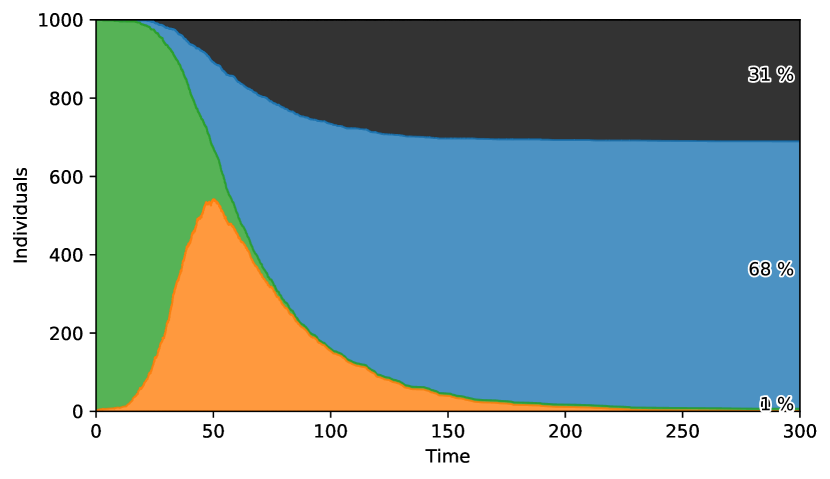
(a) SSA

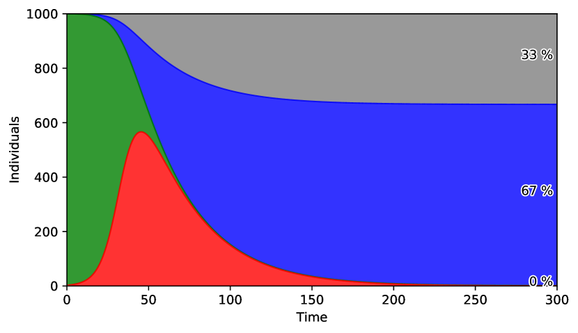
(b) ODE

Figure 5. One realisation of SSA simulation and ODE simulation for SIRD model (3.4) with basic parameters $N=1000$, $\iota=\iota^{0}=0.2$, $\rho=\rho^{0}=0.02$, $\delta=\delta^{0}=0.01$, ${I}_{0}={I}_{0}^{0}=3$.

3.1.2. Steady states of the SIR Model

Let us consider the steady states of the SIR model (3.1) which can be written as the following system of ODEs:

$$\begin{split}\frac{\mathop{}\!\mathrm{d}{\mathrm{S}}}{\mathop{}\!\mathrm{d}t}&=-\iota{\mathrm{S}}{\mathrm{I}},\\ \frac{\mathop{}\!\mathrm{d}{\mathrm{I}}}{\mathop{}\!\mathrm{d}t}&=\iota{\mathrm{S}}{\mathrm{I}}-\rho{\mathrm{I}},\;\;\\ \frac{\mathop{}\!\mathrm{d}{\mathrm{R}}}{\mathop{}\!\mathrm{d}t}&=\rho{\mathrm{I}},\end{split}$$ (3.6)

subject to initial conditions ${\mathrm{S}}(0)={\mathrm{S}}_{0}$, ${\mathrm{I}}(0)={\mathrm{I}}_{0}$ and ${\mathrm{R}}(0)={\mathrm{R}}_{0}$ for ${\mathrm{S}}_{0},{\mathrm{I}}_{0},{\mathrm{R}}_{0}\in[0,1]$. The conservation of the total number of individuals implies that ${\mathrm{S}}+{\mathrm{I}}+{\mathrm{R}}=1$ at all times $t$. Hence, the system is in fact two-dimensional and we can consider

$$\frac{\mathop{}\!\mathrm{d}{\mathrm{S}}}{\mathop{}\!\mathrm{d}t} =-\iota{\mathrm{S}}{\mathrm{I}},$$

$$\frac{\mathop{}\!\mathrm{d}{\mathrm{R}}}{\mathop{}\!\mathrm{d}t} =\rho{\mathrm{I}}.$$

We observe that

$$\frac{\mathop{}\!\mathrm{d}{\mathrm{S}}}{\mathop{}\!\mathrm{d}{\mathrm{R}}} =-\frac{\iota{\mathrm{S}}}{\rho}.$$

Any steady state $(\overline{{\mathrm{S}}},\overline{{\mathrm{I}}},\overline{{\mathrm{R}}})$ satisfies $\overline{{\mathrm{I}}}=0$, implying

$$\overline{{\mathrm{S}}}={\mathrm{S}}_{0}\exp\left(-\frac{\iota\overline{{\mathrm{R}}}}{\rho}\right)={{\mathrm{S}}_{0}}\exp\left(-\frac{\iota}{\rho}\right)\exp\left(\frac{\iota\overline{{\mathrm{S}}}}{\rho}\right)$$ (3.7)

for some constant ${{\mathrm{S}}_{0}}\in[0,1]$ where we used that $\overline{{\mathrm{S}}}+\overline{{\mathrm{R}}}=1$. Here, ${{\mathrm{S}}_{0}}$ denotes the initial condition of $\overline{{\mathrm{S}}}$, i.e. ${{\mathrm{S}}}(0)={{\mathrm{S}}_{0}}$, and implies that ${\mathrm{R}}(0)=1-{\mathrm{S}}_{0}$. Note that there exists a unique $\overline{{\mathrm{S}}}\in[0,1]$ since the left- and right-hand side of (3.7) are strictly increasing in ${\mathrm{S}}$ for ${\mathrm{S}}_{0}\in(0,1]$ and we have $0<{\mathrm{S}}_{0}\exp(-\tfrac{\iota}{\rho})$ and $1\geq{\mathrm{S}}_{0}$. Hence, $\overline{{\mathrm{R}}}\in[0,1]$ is also unique and satisfies $\overline{{\mathrm{S}}}+\overline{{\mathrm{R}}}=1$. The disease-free steady state is given by $({\mathrm{S}},{\mathrm{I}},{\mathrm{R}})=(1,0,0)$. Also note that $\overline{{\mathrm{S}}}$ is always positive for ${\mathrm{S}}_{0}>0$, which also holds for ${\mathrm{S}}(t)$, as it is monotonically decreasing in $t$ by (3.6). If the solution $({\mathrm{S}},{\mathrm{I}},{\mathrm{R}})$ becomes stationary in the long-time limit $t\to\infty$, it converges to the unique steady state $(\overline{{\mathrm{S}}},\overline{{\mathrm{I}}},\overline{{\mathrm{R}}})$. The steady states of the SIRD model can be determined in a similar way, where the disease-free steady state is given by $({\mathrm{S}},{\mathrm{I}},{\mathrm{R}},{\mathrm{D}})=(1,0,0,0)$.

3.1.3. A feature for measuring the transient phase

If the solution $({\mathrm{S}},{\mathrm{I}},{\mathrm{R}})$ for given initial data $({\mathrm{S}}_{0},{\mathrm{I}}_{0},{\mathrm{R}}_{0})$ becomes stationary in the long-time limit $t\to\infty$, it converges to the unique steady state $(\overline{{\mathrm{S}}},\overline{{\mathrm{I}}},\overline{{\mathrm{R}}})$ according to Section 3.1.2. To capture the transient phase, we derive the maximum number of infected individuals, following the approach in [11]. Due to (3.6), the necessary condition for the maximum of ${\mathrm{I}}$ satisfies

$$\frac{\mathop{}\!\mathrm{d}{\mathrm{I}}}{\mathop{}\!\mathrm{d}t}=(\iota{\mathrm{S}}-\rho){\mathrm{I}}=0.$$

Thus, ${\mathrm{S}}=\frac{\rho}{\iota}$ is a critical state and physically relevant provided $\rho\leq\iota$ so that ${\mathrm{S}}\in[0,1]$ is indeed a concentration. In this case the sufficient condition satisfies

$$\frac{\mathop{}\!\mathrm{d}^{2}{\mathrm{I}}}{\mathop{}\!\mathrm{d}t^{2}}=\iota(-\iota{\mathrm{S}}{\mathrm{I}}){\mathrm{I}}+(\iota{\mathrm{S}}-\rho)\frac{\mathop{}\!\mathrm{d}{\mathrm{I}}}{\mathop{}\!\mathrm{d}t}=-\rho\iota{\mathrm{I}}^{2}<0,$$

implying that ${\mathrm{I}}>0$ is maximal when ${\mathrm{S}}=\frac{\rho}{\iota}$. Dividing the first equation of (3.6) by ${\mathrm{S}}>0$ and integrating from $0$ to $t$ yields

$$\log{\mathrm{S}}(t)-\log{\mathrm{S}}(0)=-\iota\int_{0}^{t}{\mathrm{I}}(t^{\prime})\mathop{}\!\mathrm{d}t^{\prime}=\frac{\iota}{\rho}\int_{0}^{t}\frac{\mathop{}\!\mathrm{d}}{\mathop{}\!\mathrm{d}t^{\prime}}({\mathrm{S}}(t^{\prime})+{\mathrm{I}}(t^{\prime}))\mathop{}\!\mathrm{d}t^{\prime}=\frac{\iota}{\rho}({\mathrm{S}}(t)+{\mathrm{I}}(t)-{\mathrm{S}}(0)-{\mathrm{I}}(0)).$$ (3.8)

Here, we used in the second equality that $\frac{\mathop{}\!\mathrm{d}}{\mathop{}\!\mathrm{d}t}({\mathrm{S}}+{\mathrm{I}})=-\rho{\mathrm{I}}$ which follows from adding the first two equations of (3.6). By inserting ${\mathrm{S}}(t)=\frac{\rho}{\iota}$ and solving for ${\mathrm{I}}(t)$ we obtain that ${\mathrm{I}}(t)$ attains its maximum ${\mathrm{I}}_{\text{max}}$ satisfying

$${\mathrm{I}}_{max}=\frac{\rho}{\iota}\left(\log\frac{\rho}{\iota}-\log{\mathrm{S}}(0)-1\right)+{\mathrm{S}}(0)+{\mathrm{I}}(0).$$

Note that the transient phase for the SIRD model can be studied in a similar way and requires to replace $\rho$ in the calculations above by $\rho+\delta$.

3.1.4. $R_{0}$ and the SIR Model

The number of new infections generated by an infected person during their infectious period in a fully susceptible population is an important quantity in classic epidemiology and is referred to as $R_{0}$. The parameter $R_{0}$ characterises an infectious disease and measures the potential of disease expansion at the moment of disease introduction in a fully susceptible population. In the absence of disease, the state of the system is called disease-free equilibrium with $({\mathrm{S}},{\mathrm{I}},{\mathrm{R}})=(1,0,0)$. $R_{0}$ is related to the stability of the equilibrium, and also defines a transcritical bifurcation where the disease-free equilibrium changes from being stable, i.e. the disease fails to invade, to being unstable, i.e. the disease starts expanding exponentially. When disease transmission is modeled by a system of ODEs, such as in (3.6), the eigenvalues of the linearisation at the disease-free equilibrium are related to $R_{0}$ in a straightforward way: $R_{0}>1$ is equivalent to at least one eigenvalue being positive.

As a simple example of the direct calculation of $R_{0}$, we write the infection rate $\iota$ as a product of the number of contacts an individual has per unit time, denoted by the encounter rate $\beta$, and the probability $p$ of infection given an encounter. This allows us to write $\iota=\beta\,p$ and the SIR model (3.6) can be written as

$$\frac{\mathop{}\!\mathrm{d}{\mathrm{S}}}{\mathop{}\!\mathrm{d}t} =-{\beta}p{\mathrm{I}}{\mathrm{S}}$$

$$\frac{\mathop{}\!\mathrm{d}{\mathrm{I}}}{\mathop{}\!\mathrm{d}t} ={\bf\beta}p{\mathrm{I}}{\mathrm{S}}-\rho{\mathrm{I}}$$

$$\frac{\mathop{}\!\mathrm{d}{\mathrm{R}}}{\mathop{}\!\mathrm{d}t} =\rho{\mathrm{I}}.$$

The probability $p$ can be further decomposed into

$$p=si,$$ (3.9)

where the susceptibility $s$ measures the risk of getting infected by an encounter, and the infectivity $i$ describes the chance of infection.

At the disease free equilibrium with ${\mathrm{S}}=1$, we can approximate the dynamics of the infected population as

$$\frac{\mathop{}\!\mathrm{d}{\mathrm{I}}}{\mathop{}\!\mathrm{d}t} =\left({\beta}p-\rho\right){\mathrm{I}}$$

with solution

$${\mathrm{I}}(t) ={\mathrm{I}}_{0}\exp(\left({\beta}p-\rho\right)t)$$

for initial data ${\mathrm{I}}(0)={\mathrm{I}}_{0}$. Hence, the associated eigenvalue of the linearisation is given by $\beta p-\rho$ and the positivity of $\beta p-\rho>0$ is equivalent to

$$R_{0}=\frac{{\beta}p}{\rho}>1,$$

based on the equivalence mentioned above. Notice that $R_{0}$ can be regarded as the product of the three factors $\beta$, $p$ and $\tfrac{1}{\rho}$ which correspond to the three fundamental ways by which disease transmission can be controlled: decreasing the number $\beta$ of contacts, decreasing the probability $p$ of infection for every contact (for instance by using masks) and decreasing the infectious period (for instance via disease treatment). This is consistent with the definition of $R_{0}$ by the largest eigenvalue of the next-generation matrix (NGM) which we denote by $K$ in the following. For techniques to determine $R_{0}$, see [19]. In our simple case,

$$K=\frac{\iota}{\rho}=\frac{\beta p}{\rho}$$

is a 1$\times$1-matrix obtained from the infected subsystem of (3.6). Thus,

$$R_{0}=\frac{\iota}{\rho}=\frac{\beta p}{\rho}.$$

When including types and rules for deceased individuals in the SIRD model, we derive the basic reproduction number $R_{0}$ analogously by replacing $\rho$ with total removement rate $\rho+\delta$. Thus we get for the basic parameter setting

$$R_{0}=\frac{\iota^{0}}{\rho^{0}+\delta^{0}}=\frac{0.2}{0.02+0.01}=6\frac{2}{3}.$$ (3.10)

The basic reproduction number $R_{0}$ not only describes the beginning of epidemics. $R_{0}$ can also be used directly for simple cases to describe the fraction of susceptible individuals that survive without any infection. Considering the limit for $t\rightarrow\infty$ in (3.8), where we set ${\mathrm{I}}(0)=0$, $\lim_{t\to\infty}{\mathrm{I}}(t)=0$ and ${\mathrm{S}}(0)=1$, yields

$$\lim_{t\to\infty}{\mathrm{S}}(t)=\exp\left(-R_{0}(1-\lim_{t\to\infty}{\mathrm{S}}(t)\right).$$ (3.11)

(3.11) is called final size relation [11], for a meaning-full stochastic derivation, see [53]. Note that (3.11) is robust to changes within the course of the epidemic.

We can also consider the time-dependent number of new infections an infected individual can generate while infectious and the disease is expanding or established in a population, this is, when susceptible individuals are no longer the whole population. We denote this quantity by $R_{\text{eff}}$ and write $R_{\text{eff}}=S(t)R_{0}$, i.e.

$$R_{\text{eff}}(t)=\frac{\beta p{\mathrm{S}}(t)}{\rho}.$$

In this case, an infectious individual encounters fewer susceptible individuals per unit time at an average rate $\beta\,{\mathrm{S}}(t)$.

One possibility to estimate $R_{\text{eff}}$ from data is to fit a model and determine the specific value for $R_{0}$ based on the estimated parameters. A more frequently used method [17] is to estimate $R_{0}$ directly from data, e.g. by considering incidences and serial data. The German RKI [2] considers the daily reported new cases $I_{t}^{\text{new}}$ at time $t$ and estimates $R_{\text{eff}}$ from the number of infections within the last four days as

$$\widetilde{R}_{\text{eff}}(t)=\frac{\sum_{s=t-6}^{t}I_{s}^{\text{new}}}{\sum_{s=t-6}^{t}I_{s-4}^{\text{new}}}.$$

3.2. Age

We make the standard SIR model a bit more realistic by introducing discrete age classes which can vary in vulnerability with respect to the coronavirus. Age was a key factor of individual vulnerability, recognised already at the early stages of the COVID-19 pandemic.

Table 2. The types of the adapted COVID-19 age class structured SIRD model.

Types	Interpretation
$S_{a},a\in A$	Susceptible	individuals of age class $a$
$I_{a},a\in A$	Infectious	individuals of age class $a$
$R_{a},a\in A$	Recovered	individuals of age class $a$
$D_{a},a\in A$	Individuals that have died within age class $a$

For reaction constants $\iota_{a,a^{\prime}},\rho_{a},\delta_{a}>0$, $a,a^{\prime}\in A$, the following rules describe type changes:

$$S_{a}+I_{a^{\prime}} $\displaystyle\xrightarrow{\iota_{a,a'}}$\hfil\ignorespaces I_{a}+I_{a^{\prime}}, \quad a,a^{\prime}\in A$$    [Infections] (3.12)

$$I_{a} $\displaystyle\xrightarrow{\rho_{a}}$\hfil\ignorespaces R_{a}, \quad a\in A$$    [Recovery]

$$I_{a} $\displaystyle\xrightarrow{\delta_{a}}$\hfil\ignorespaces D_{a}, \quad a\in A$$    [Death]

Here, the infectious rates $\iota_{a,a^{\prime}}$ control the rate of spread, i.e. $\iota_{a,a^{\prime}}$ represents the probability of transmitting the disease between a susceptible of age class $a$ and an infectious individual of age class $a^{\prime}$. The recovery rates $\rho_{a}$ and death rates $\delta_{a}$ are related to the average duration $\tau_{a}$ of the infection for age class $a$ by $\rho_{a}+\delta_{a}=1/\tau_{a}$. We assume lower recovery rates for higher age classes, as older individuals may suffer longer from COVID-19, and higher death rates $\delta_{a}$ for older age classes, as the probability to die is much higher.

The NGM for age model (using again Diekmann splitting [19]) is given by:

$$K=K_{L}=\begin{pmatrix}p_{1}&\ldots&0\\ \vdots&\ddots&\vdots\\ 0&\ldots&p_{n_{a}}\end{pmatrix}\begin{pmatrix}\iota_{1,1}&\ldots&\iota_{1,n_{a}}\\ \vdots&\ddots&\vdots\\ \iota_{n_{a},1}&\ldots&\iota_{n_{a},n_{a}}\end{pmatrix}\begin{pmatrix}\frac{1}{\rho_{1}+\delta_{1}}&\ldots&0\\ \vdots&\ddots&\vdots\\ 0&\ldots&\frac{1}{\rho_{n_{a}}+\delta_{n_{a}}}\end{pmatrix},$$

where $p_{a}$ is the fraction of all individuals in age class $a$.

Besides recovery and death, age creates heterogeneity by structuring these groups by different contact rates and infectivity. Thus the infection rate matrix becomes dependent on susceptibility $s_{a}$, infectivity $i_{a}$ and contacts $C_{a,a^{\prime}}$ of the respective age classes $a,a^{\prime}$

$$\iota_{a,a^{\prime}}=q\cdot s_{a}\cdot i_{a^{\prime}}\cdot C_{a,a^{\prime}},$$ (3.13)

where $q$ is a calibration factor accounting for parameters on the same time scale. Note that by different values for susceptibility and infectivity the infection matrix is not necessarily symmetric. For these simple models we assume constant contact matrices, which of course is not very realistic as behaviour induced by the epidemic changes contacts.

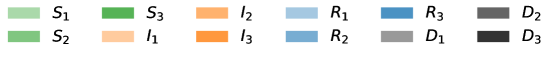
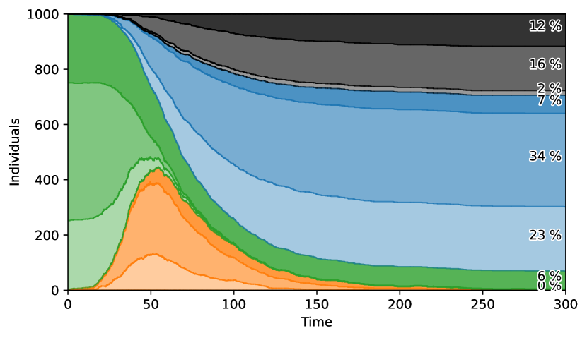
(a) contact $100\%$, $R_{0}\approx 6.66$

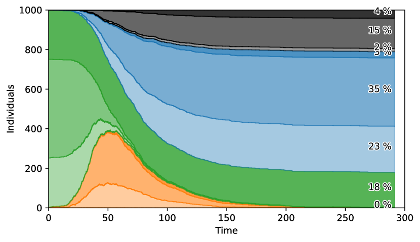
(b) contact reduction of $80\%$ with oldest age class, $R_{0}\approx 6.59$

Figure 6. SSA simulations for SIRD model with age including contact matrices. $\rho=\rho^{0}(1.5,1.0,0.5)$, $\delta=\delta^{0}(0.25,1.0,2.)$, $p=(0.25,0.5,0.25)$.

For the simulations in Figure 6 we assumed for reasons of simplification constant susceptibility and infectivity but different parameters for recovery and death. We choose the contact matrix $C$ based on condensed and symmetrised results by [67], see also [54, 38, 61]

$$C=\begin{pmatrix}76&38&5\\ 38&67&13\\ 5&13&9\end{pmatrix}$$

and the calibration factor $q$ such that the basis reproduction number in Figure 6(a) equals $R_{0}$ of the basis case (3.10), see Figure 5. Here we observe the hidden heterogeneity reducing the maximum number of infected, but also less recovery and larger fatality for the oldest age group increasing their death fraction to almost half of the beginning. In Figure 6(b) we kept the calibration and all other parameters unchanged but modeling saving vulnerable groups, here the elderly, by young and middle aged reducing contacts with them by $80\%$. This results in a marginally smaller value for $R_{0}$ but in a significantly smaller number for fatalities in the oldest group.

3.3. Testing

A variation of the $SIR$-model for COVID-19 application is the distinction into tested and untested individuals in a certain disease state. The idea gives rise to Table 3. Due to the development of tests for COVID-19, many countries introduced testing strategies and based their policy decisions on their testing efforts. Therefore, we need a modelling tool that incorporates this extended classification scheme. It turns out that the distinction into different test classes introduces a combinatorial extension of the $SIR$ rules.

Table 3. The types of the standard SIR model with differentiation into untested, tested and tested but changed cases.

Type	Interpretation
$c\in\{0,1,2\}$	Sub-type for test status:	$0$: untested,
		$1$: tested,
		$2$: tested but unawarely changed disease status
$S_{c}$	Susceptible individuals	of test class $c$
$I_{c}$	Infectious individuals	of test class $c$
$R_{c}$	Recovered individuals	of test class $c$
$D_{c}$	Deceased individuals	of test class $c$

The introduction of individuals tested but unawarely changed disease status $I_{2}$ in the classification in Table 3 is due the fact, that freshly tested susceptible individuals might get infected without knowing and before getting the next test. Thus they might behave and are allowed to behave like negatively tested susceptibles. The proposed rules can be described as follows:

$$S_{0}+I_{0} $\displaystyle\xrightarrow{\iota_{0,0}}$\hfil\ignorespaces I_{0}+I_{0}$$ [Untested Infections] (3.14)

$$S_{1}+I_{0} $\displaystyle\xrightarrow{\iota_{1,0}}$\hfil\ignorespaces I_{2}+I_{0}$$ [Cross Infections I]

$$S_{0}+I_{1} $\displaystyle\xrightarrow{\iota_{0,1}}$\hfil\ignorespaces I_{0}+I_{1}$$ [Cross Infections II]

$$S_{1}+I_{1} $\displaystyle\xrightarrow{\iota_{1,1}}$\hfil\ignorespaces I_{2}+I_{1}$$ [Tested Infections]

$$S_{0}+I_{2} $\displaystyle\xrightarrow{\iota_{0,2}}$\hfil\ignorespaces I_{0}+I_{2}$$ [Cross Infections III]

$$S_{1}+I_{2} $\displaystyle\xrightarrow{\iota_{1,2}}$\hfil\ignorespaces I_{2}+I_{2}$$ [Cross Infections IV]

$$I_{0} $\displaystyle\xrightarrow{\rho_{0}}$\hfil\ignorespaces R_{0}$$ [Untested Recovery]

$$I_{1} $\displaystyle\xrightarrow{\rho_{1}}$\hfil\ignorespaces R_{1}$$ [Tested Recovery]

$$I_{2} $\displaystyle\xrightarrow{\rho_{2}}$\hfil\ignorespaces R_{2}$$ [Tested Recovery II]

$$I_{0} $\displaystyle\xrightarrow{\delta_{0}}$\hfil\ignorespaces D_{0}$$ [Death, Untested]

$$I_{1} $\displaystyle\xrightarrow{\delta_{1}}$\hfil\ignorespaces D_{1}$$ [Death, Tested]

$$I_{2} $\displaystyle\xrightarrow{\delta_{2}}$\hfil\ignorespaces D_{2}$$ [Death, Tested II]

$$S_{0} $\displaystyle\xrightarrow{\vartheta_{S}}$\hfil\ignorespaces S_{1}$$ [Testing, Susceptibles]

$$I_{0} $\displaystyle\xrightarrow{\vartheta_{I}}$\hfil\ignorespaces I_{1}$$ [Testing, Infected]

$$R_{0} $\displaystyle\xrightarrow{\vartheta_{R}}$\hfil\ignorespaces R_{1}$$ [Testing, Recovered]

$$S_{1} $\displaystyle\xrightarrow{\lambda}$\hfil\ignorespaces S_{0}$$ [Loss of Information, tested Susceptibles]

$$I_{2} $\displaystyle\xrightarrow{\lambda}$\hfil\ignorespaces I_{0}$$ [Loss of Information, tested unawarely Infected]

$$R_{2} $\displaystyle\xrightarrow{\lambda}$\hfil\ignorespaces R_{0}$$ [Loss of Information, tested unawarely Recovered]

The first six rules in (3.14) describe the simple $SIR$ infection process, where now infections are differentiated into infections of untested, tested and tested but unawarely infected individuals. Rules [Cross Infections I], [Tested Infections] and [Cross Infections IV] model the potentially dangerous case when a tested susceptible individual with less restrictions is unknowingly infected. We assume here that there is just one universal test which has 100% accuracy of detecting the disease status of an individual. The base infection rates $\iota_{c,c^{\prime}}>0$, $c\in\{0,1\}$, $c^{\prime}\in\{0,1,2\}$ may be different because tested cases may show different behaviour or are restricted in some way, for example by staying in quarantine or hospital. The next three rules in (3.14) with rates $\rho_{c}$ > 0, $c\in\{0,1,2\}$ are physiological rules describing the recovery. Here we assume that recovery in contrast to infection is a conscious process, therefore the tested infected turn into tested recovered. Basically no differentiation between tested or untested individuals is needed, but for tested infected we may assume, that based on the correct classification the individuals may increase their recovery. Whereas infected individuals $I_{2}$, who think they are just susceptible may misinterpret symptoms. Thus $\rho_{1}\geq\rho_{2}\geq\rho_{0}$. Similar arguments hold for the decrease of the risk to die for the following three rules with rates $0<\delta_{1}\leq\delta_{0}\leq\delta_{2}$. In the next three rules in (3.14) we introduce a testing procedure which is modelled as an urn model and where susceptible, infected and recovered individuals are tested with rates $\vartheta_{S}>0$, $\vartheta_{I}>0$ and $\vartheta_{R}>0$, respectively. The rates $\vartheta_{S}$, $\vartheta_{I}$ and $\vartheta_{R}$ may be different because infected individuals may show symptoms which lead to increased testing of infected individuals. Deceased individuals are not tested, but keep their respective test status. The final three rules for tested susceptible individuals, or infected or recovered individuals, who think they are susceptible, describe the decreasing trust in the result requiring a new test with rate $\lambda>0$ or, by deterministic updates, the limited validity period of a test. For tested infected and recovered individuals we assume perfect preserving and tracing of information, thus they keep their tested status as we do not include loss of immunity. The rules in (3.14) can be summarised as

$$S_{0}+I_{c^{\prime}} $\displaystyle\xrightarrow{\iota_{0, c'}}$\hfil\ignorespaces I_{0}+I_{c^{\prime}}, \quad c^{\prime} \in\{0,1,2\}\quad$$ [Infections] (3.15)

$$S_{1}+I_{c^{\prime}} $\displaystyle\xrightarrow{\iota_{1, c'}}$\hfil\ignorespaces I_{2}+I_{c^{\prime}}, \quad c^{\prime} \in\{0,1,2\}\quad$$ [Infections]

$$I_{c} $\displaystyle\xrightarrow{\rho_{c}}$\hfil\ignorespaces R_{c}, \quad c \in\{0,1,2\}\quad$$ [Recovery]

$$I_{c} $\displaystyle\xrightarrow{\delta_{c}}$\hfil\ignorespaces D_{c}, \quad c \in\{0,1,2\}\quad$$ [Death]

$$X_{0} $\displaystyle\xrightarrow{\vartheta_{X}}$\hfil\ignorespaces X_{1}, \quad X \in\{S,I,R\}\quad$$ [Testing]

$$S_{1} $\displaystyle\xrightarrow{\lambda}$\hfil\ignorespaces S_{0},$$ [Loss of Information,

tested Susceptible]

$$X_{2} $\displaystyle\xrightarrow{\lambda}$\hfil\ignorespaces X_{0}, \quad X \in\{I,R\}\quad$$ [Loss of Information,

tested unawarely Infected / Recovered]

The ODE system associated with the rules in (3.15) is given by (3.16), the propensities are derived as in the other models and therefore omitted.

$$\frac{\mathop{}\!\mathrm{d}{\mathrm{S}}_{c}}{\mathop{}\!\mathrm{d}t} =-{\mathrm{S}}_{c}\sum_{c^{\prime}\in\{0,1,2\}}\iota_{c,c^{\prime}}{\mathrm{I}}_{c^{\prime}}-(-1)^{c}(\vartheta_{S}{\mathrm{S}}_{0}-\lambda{\mathrm{S}}_{1}),\enspace c\in\{0,1\},$$ (3.16)

$$\frac{\mathop{}\!\mathrm{d}{\mathrm{S}}_{2}}{\mathop{}\!\mathrm{d}t} =0,$$

$$\frac{\mathop{}\!\mathrm{d}{\mathrm{I}}_{0}}{\mathop{}\!\mathrm{d}t} ={\mathrm{S}}_{0}\sum_{c^{\prime}\in\{0,1,2\}}\iota_{0,c^{\prime}}{\mathrm{I}}_{c^{\prime}}-(\rho_{0}+\delta_{0}){\mathrm{I}}_{0}-\vartheta_{I}{\mathrm{I}}_{0}+\lambda{\mathrm{I}}_{2}),$$

$$\frac{\mathop{}\!\mathrm{d}{\mathrm{I}}_{1}}{\mathop{}\!\mathrm{d}t} =-(\rho_{1}+\delta_{1}){\mathrm{I}}_{1}+\vartheta_{I}{\mathrm{I}}_{0},$$

$$\frac{\mathop{}\!\mathrm{d}{\mathrm{I}}_{2}}{\mathop{}\!\mathrm{d}t} ={\mathrm{S}}_{1}\sum_{c^{\prime}\in\{0,1,2\}}\iota_{1,c^{\prime}}{\mathrm{I}}_{c^{\prime}}-(\rho_{2}+\delta_{2}){\mathrm{I}}_{2}-\lambda{\mathrm{I}}_{2},$$

$$\frac{\mathop{}\!\mathrm{d}{\mathrm{R}}_{0}}{\mathop{}\!\mathrm{d}t} =\rho_{0}{\mathrm{I}}_{0}-\vartheta_{R}{\mathrm{R}}_{0}+\lambda{\mathrm{R}}_{2},$$

$$\frac{\mathop{}\!\mathrm{d}{\mathrm{R}}_{1}}{\mathop{}\!\mathrm{d}t} =\rho_{1}{\mathrm{I}}_{1}+\vartheta_{R}{\mathrm{R}}_{0},$$

$$\frac{\mathop{}\!\mathrm{d}{\mathrm{R}}_{2}}{\mathop{}\!\mathrm{d}t} =\rho_{2}{\mathrm{I}}_{2}-\lambda{\mathrm{R}}_{2},$$

$$\frac{\mathop{}\!\mathrm{d}{\mathrm{D}}_{c}}{\mathop{}\!\mathrm{d}t} =\delta_{c}{\mathrm{I}}_{c},$$

$$\frac{\mathop{}\!\mathrm{d}{\mathrm{D}}_{2}}{\mathop{}\!\mathrm{d}t} =\delta_{2}{\mathrm{I}}_{2},$$

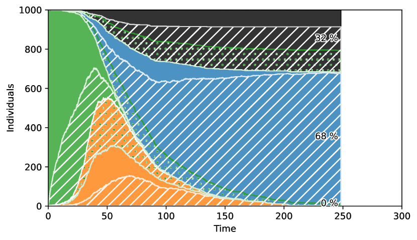
(a) SSA, $\lambda=0.02$, pure testing

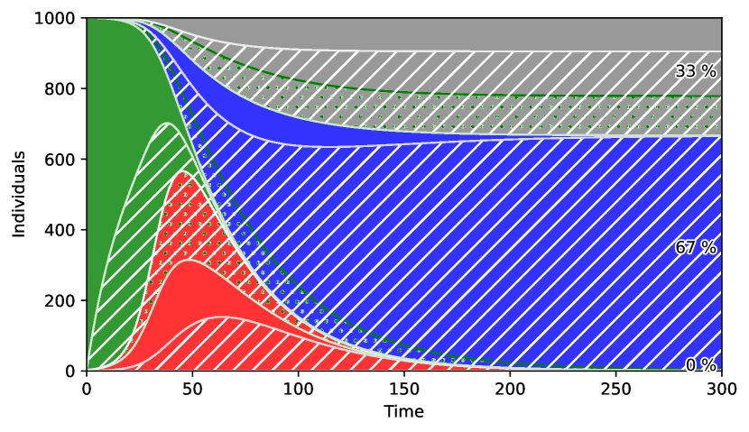
(b) ODE, $\lambda=0.02$, pure testing

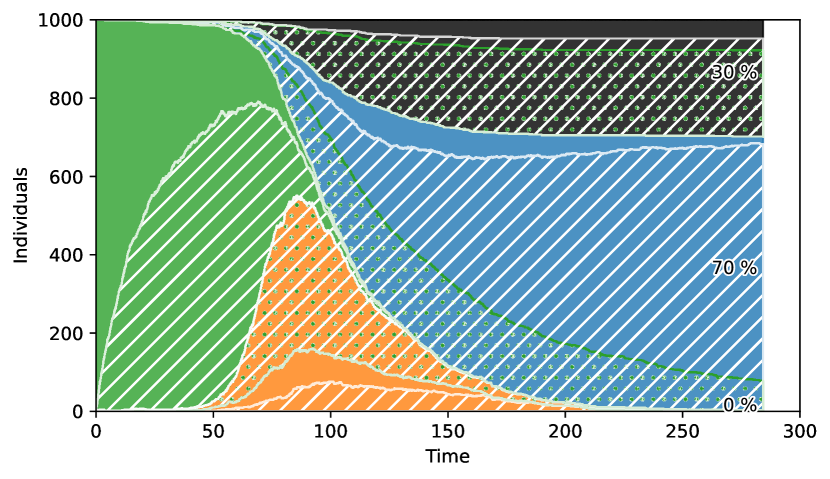
(c) SSA, $\lambda=0.02$, restrictions

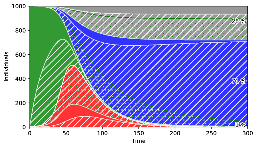
(d) ODE, $\lambda=0.02$, restrictions

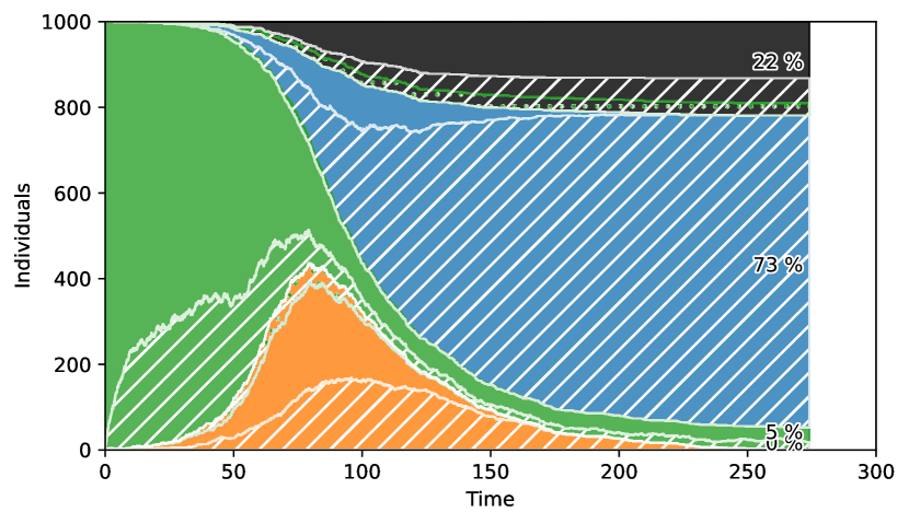
(e) SSA, $\lambda=0.2$, restrictions

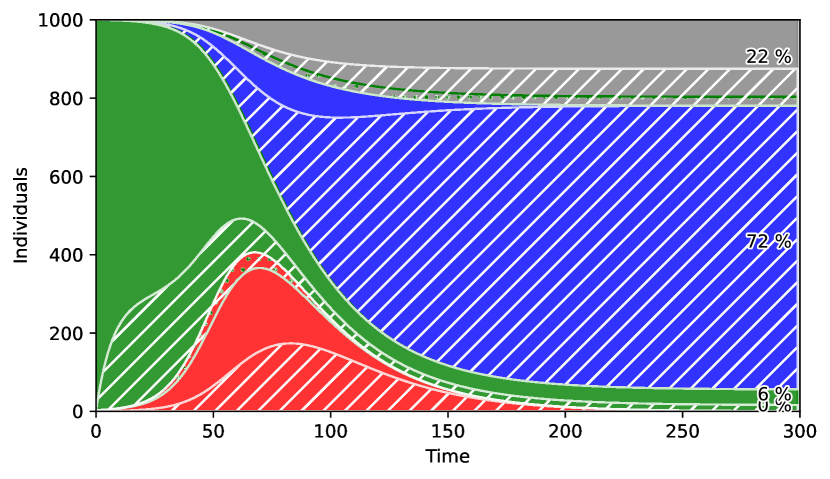
(f) ODE, $\lambda=0.2$, restrictions

Figure 7. SSA and ODE simulations for SIRD model with testing and different rates of loss of information $\lambda$. ${\vartheta_{S}=\vartheta_{I}=\vartheta_{R}=\vartheta=0.04}$. For 7(a), 7(b): ${\iota=\iota^{0}\left(\begin{smallmatrix}1.&1.&1.\\ 1.&1.&1.\end{smallmatrix}\right)}$ ${\rho=\rho^{0}(1.,1.,1.)}$, ${\delta=\delta^{0}(1.,1.,1.)}$. For 7(c)-7(f): ${\iota=\iota^{0}\left(\begin{smallmatrix}0.7&0.2&0.9\\ 0.9&0.2&1.\end{smallmatrix}\right)}$, ${\rho=\rho^{0}(1.,1.5,1.)}$, ${\delta=\delta^{0}(1.0,0.5,1.0)}$.

Figure 7(b) shows the ODE simulation for the same parameters as for the SIRD base case in Figure 5(b) only with added testing in whitish hatches and green dotted hatches for unawarely infected tested individuals. The SSA simulation in Figure 7(a) differs from 5(b) because of stochasticity. Both show that for a moderate testing rate $\vartheta=0.04$ and minor loss rate $\lambda=0.02$, the number of unawarely infected tested is high. Since the infection parameters are those of the base case this has no consequences. The simulations in Figures 7(c) and 7(d) are for the same testing parameters but including restrictions for tested infected or untested individuals by multiplying the base infection rate with a matrix, as well as the influence of testing on treatment and thus increased chance of recovery and decreased risk of dying. Because the huge amount of unawarely infected tested individuals can act as freely as tested uninfected, it affects the number of death by increasing its toll and the benefit of testing almost vanishes. Reducing the validity period of tests by increasing the loss rate in Figures 7(e) and 7(f) increases the efficiency of test and the number of unawarely infected tested individuals is almost negligible. This results in a flatter curve of infected and reduced share of deceased. Also a remarkable amount of susceptibles survive the disease without ever getting infected. This model for testing shows, that (presumably) knowing the disease status with according behaviour works only well when the validity period of the test is not too long but coupled with the infectious period or at least latent period of the virus.

3.4. Global Information and State Dependent Rates

One aspect making pandemics in the 21st century different from pandemics in previous centuries is the availability of data on the disease, from local to even global levels. We discuss a simple $SIRD$-model which incorporates this data with the help of global information functional responses, see Section 2.1.1. For the classification, we use Table 1. The rules now incorporate functional responses:

$$S+I $\displaystyle\xrightarrow{\iota(S, I, R, D; \mu)}$\hfil\ignorespaces I+I$$    [Infection] (3.17)

$$I $\displaystyle\xrightarrow{\rho}$\hfil\ignorespaces R$$    [Recovery]

$$I $\displaystyle\xrightarrow{\delta}$\hfil\ignorespaces D$$    [Death]

Here, we suppose that the infection rate $\iota$ may depend on $S,I,R,D$ as well as additional parameters summarised in the variable $\mu$. We assume that $\iota$ is monotonically increasing in $S$ and $R$, modelling that if the population registers many unharmed (but susceptible) and recovered individuals, the population in general becomes more careless. We assume that $\iota$ is monotonically decreasing in $I$ and $D$, modelling that if the population detects more infected, or even dead individuals, then the population in general becomes more careful in behavioural terms. In this simple model the infection rate in the form of a functional response reduces to

$$\iota({I};\mu)=\frac{\iota_{0}}{1+\mu\frac{{I}}{N}}\quad\text{(used in propensities),}\quad\iota({\mathrm{I}};\mu)=\frac{\iota_{0}}{1+\mu{\mathrm{I}}}\quad\text{(used in ODEs),}$$

where $\mu$ is a non-negative parameter that models the severity of contact reductions. Note that this function works as a self-regulator: for increasing numbers ${I}$, individuals may become more cautious and follow social distancing rules which may lead to a decreasing infection rate $\iota$ and a decrease of the number of newly infected individuals, while at a later point in time the infections may rise again. This results in the following propensities for numbers ${\mathrm{S}},{\mathrm{I}},{\mathrm{R}},{\mathrm{D}}$ of individuals and the associated concentrations ${S},{I},{R},{D}$:

Propensities with numbers:

$$\kappa_{1}({S},{I},{R},{D}) =\frac{\iota({S},{I},{R},{D};\mu)}{N}{S}{I},$$ (3.18)

$$\kappa_{2}({S},{I},{R},{D}) =\rho{I},$$

$$\kappa_{3}({S},{I},{R},{D}) =\delta{I}.$$

ODEs with fractions:

$$\frac{\mathop{}\!\mathrm{d}{\mathrm{S}}}{\mathop{}\!\mathrm{d}t} =-\iota({\mathrm{S}},{\mathrm{I}},{\mathrm{R}},{\mathrm{D}};\mu){\mathrm{S}}{\mathrm{I}},$$ (3.19)

$$\frac{\mathop{}\!\mathrm{d}{\mathrm{I}}}{\mathop{}\!\mathrm{d}t} =\iota({\mathrm{S}},{\mathrm{I}},{\mathrm{R}},{\mathrm{D}};\mu){\mathrm{S}}{\mathrm{I}}-(\rho+\delta){\mathrm{I}},$$

$$\frac{\mathop{}\!\mathrm{d}{\mathrm{R}}}{\mathop{}\!\mathrm{d}t} =\rho{\mathrm{I}},$$

$$\frac{\mathop{}\!\mathrm{d}{\mathrm{D}}}{\mathop{}\!\mathrm{d}t} =\delta{\mathrm{I}}.$$

Note that (3.19) always conserves the concentration of all individuals, i.e.

$${\mathrm{S}}(t)+{\mathrm{I}}(t)+{\mathrm{R}}(t)+{\mathrm{D}}(t)=1$$ (3.20)

for all times $t\geq 0$. We assume that infection rate $\iota({\mathrm{I}},{\mathrm{R}},{\mathrm{D}};\mu)$ is a positive, differentiable function of ${\mathrm{I}}$, ${\mathrm{R}}$ and ${\mathrm{D}}$ which increases with respect to ${\mathrm{R}}$ and decreases with respect to ${\mathrm{I}}$ and ${\mathrm{D}}$:

$$\frac{\partial\iota({\mathrm{I}},{\mathrm{R}},{\mathrm{D}};\mu)}{\partial{\mathrm{R}}}>0\mbox{ for all $({\mathrm{R}},{\mathrm{I}},{\mathrm{D}})\in[0,1]^{3}$ and $\mu\in\mathbb{R}^{\ell}$},$$ (3.21)

$$\frac{\partial\iota({\mathrm{I}},{\mathrm{R}},{\mathrm{D}};\mu)}{\partial{\mathrm{I}}}<0\mbox{ for all $({\mathrm{R}},{\mathrm{I}},{\mathrm{D}})\in[0,1]^{3}$ and $\mu\in\mathbb{R}^{\ell}$},$$

$$\frac{\partial\iota({\mathrm{I}},{\mathrm{R}},{\mathrm{D}};\mu)}{\partial{\mathrm{D}}}<0\mbox{ for all $({\mathrm{R}},{\mathrm{I}},{\mathrm{D}})\in[0,1]^{3}$ and $\mu\in\mathbb{R}^{\ell}$}.$$

The conditions (3.21) describe the effects of available information:

• the more recovered individuals exist, the more there is an increase of interactions among individuals and thus increasing infectivity.

• The more infections the more appears a tendency to decrease of interactions among individuals and thus decreasing infectivity.

• The more deaths the more appears a tendency to decrease of interactions among individuals and thus decreasing infectivity.

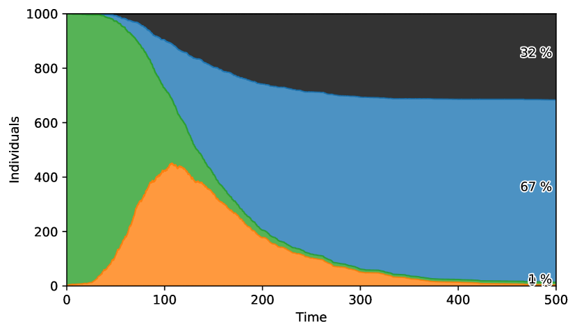
(a) SSA, $N=1000$, $\mu=1$

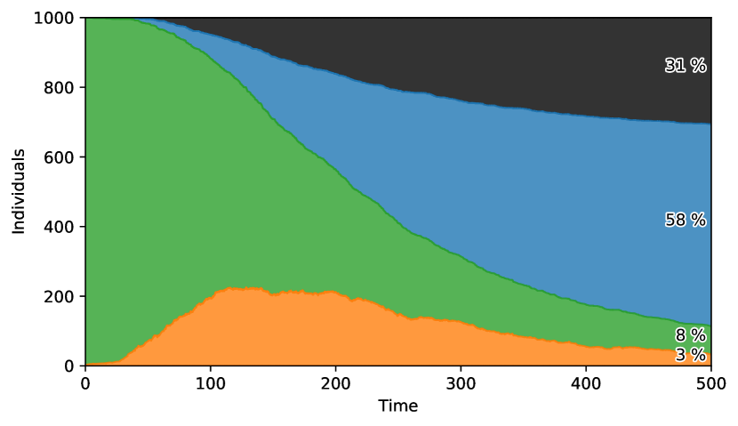
(b) SSA, $N=1000$, $\mu=10$

Figure 8. SSA simulations for SIRD model with functional response, for base case parameters and simple saturation $\iota({I};\mu)=\frac{\iota^{0}}{1+\mu\frac{{I}}{N}}$ for different $\mu$.

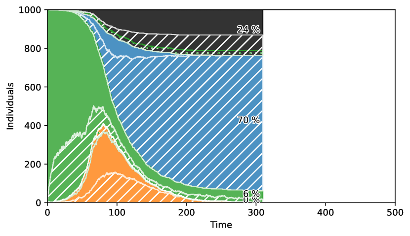
(a) SSA, $N=1000$, $\mu=1$

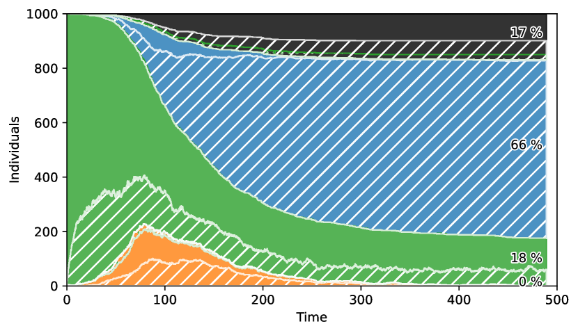
(b) SSA, $N=1000$, $\mu=10$

Figure 9. SSA simulations for SIRD model with testing (minor testing $\vartheta$, higher loss $\lambda$) and functional response, simple saturation $\iota({I};\mu)=\frac{\iota^{0}}{1+\mu\frac{{I}_{1}}{N}}$ for different response $\mu\in\mathbb{R}$, loss of testing information rate $\lambda=0.1$, for further parameters see also Figure 7.

For simulations by SSA for $\mu=1$ and $\mu=10$, see Figure 8. Note that here the maximum time is set to $T=500$. Even more realistic, we model the global information based on the number of tested infectious individuals ${I}_{1}$ by combining (3.14) and (3.17). Numerical results for this model are shown in Figure 9. Comparing Figure 9(b) to Figure 5(a) it is possible to observe that testing and global information lead to a more effective flattening the curve of the infected cases and lowering the death toll. The contribution of testing can be seen by considering Figure 8(b) where the death exceeds the level of Figure 9(b).

Note that the shape of the hashed parts of Figure 9 look similar to Figure 8. The number of unrecorded cases are obviously greater for global information dependent on tested cases, but can be controlled with appropriate behaviour $\mu$.

3.4.1. Steady states

In this subsection we want to explore a simple model aiming to study what can be called global information, namely the fact that the knowledge of $I$, $R$ and $D$ may influence the behaviour of many individuals who may try to adjust their actions (e.g. social distancing, precaution measures, etc.), in order to minimise their risk of infection. To this end we require an infection rate depending upon infectious cases $I$, recovered cases $R$ and dead cases $D$. In particular we study the dependence of the maximum of the infection on the form infection rate. We make the following assumptions:

• the information is available uniformly in the population,

• the information affects the rates instantaneously.

Consider a SIR model with $({\mathrm{S}},{\mathrm{I}},{\mathrm{R}},{\mathrm{D}})\in[0,1]^{4}$ with an infection rate $\iota({\mathrm{I}},{\mathrm{R}},{\mathrm{D}};\mu)$ as a smooth function of ${\mathrm{I}}$, ${\mathrm{R}}$, ${\mathrm{D}}$ and a set of parameters denoted by a vector $\mu\in\mathbb{R}^{\ell}$ for some $\ell\geq 1$. Following the notation in the previous section we consider the infection rate $\iota({\mathrm{I}},{\mathrm{R}},{\mathrm{D}};\mu)$ which results in a SIRD model with state dependent infection rate:

$$\begin{split}&\frac{\mathop{}\!\mathrm{d}{\mathrm{S}}}{\mathop{}\!\mathrm{d}t}=-\iota({\mathrm{I}},{\mathrm{R}},{\mathrm{D}};\mu)\,{\mathrm{S}}\,{\mathrm{I}},\\ &\frac{\mathop{}\!\mathrm{d}{\mathrm{I}}}{\mathop{}\!\mathrm{d}t}=\iota({\mathrm{I}},{\mathrm{R}},{\mathrm{D}};\mu)\,{\mathrm{S}}\,{\mathrm{I}}-\rho\,{\mathrm{I}}-\delta\,{\mathrm{I}},\\ &\frac{\mathop{}\!\mathrm{d}{\mathrm{R}}}{\mathop{}\!\mathrm{d}t}=\rho\,{\mathrm{I}},\\ &\frac{\mathop{}\!\mathrm{d}{\mathrm{D}}}{\mathop{}\!\mathrm{d}t}=\delta\,{\mathrm{I}}.\end{split}$$ (3.22)

The steady states $(\bar{\mathrm{S}},\bar{\mathrm{I}},\bar{\mathrm{R}},\bar{\mathrm{D}})$ are characterised by the conditions

$$\overline{{\mathrm{I}}}=0,\qquad\overline{{\mathrm{S}}}+\overline{{\mathrm{R}}}+\overline{{\mathrm{D}}}=1,$$

implying that all steady states are infectious free states. Under the above assumptions on $\iota$, (3.22) has a unique solution ${\mathrm{S}}(t),{\mathrm{I}}(t),{\mathrm{R}}(t),{\mathrm{D}}(t)$ which depends continuously on $\mu$. By (3.22) there exists a manifold $\Sigma$ of states satisfying $\frac{\mathop{}\!\mathrm{d}{\mathrm{I}}}{\mathop{}\!\mathrm{d}t}=0$ and given by

$$\iota({\mathrm{I}},{\mathrm{R}},{\mathrm{D}};\mu)\,{\mathrm{S}}-\rho-\delta=0,\quad{\mathrm{S}}+{\mathrm{I}}+{\mathrm{R}}+{\mathrm{D}}=1.$$

Equivalently, $\Sigma$ can be characterised by the single equation

$$\iota({\mathrm{I}},{\mathrm{R}},{\mathrm{D}};\mu)\,(1-{\mathrm{I}}-{\mathrm{R}}-{\mathrm{D}})-\rho-\delta=0.$$ (3.23)

Under appropriate assumptions on $\iota$, e.g. $\rho+\delta\leq\iota({\mathrm{I}},{\mathrm{R}},{\mathrm{D}};\mu)$ for all ${\mathrm{I}},{\mathrm{R}},{\mathrm{D}}$ as in Section 3.1.3, a solution to (3.23) is guaranteed. Using (3.22), we obtain

$$\frac{\mathop{}\!\mathrm{d}^{2}{\mathrm{I}}}{\mathop{}\!\mathrm{d}t^{2}} =\frac{\mathop{}\!\mathrm{d}{\mathrm{I}}}{\mathop{}\!\mathrm{d}t}(\iota({\mathrm{I}},{\mathrm{R}},{\mathrm{D}};\mu)\,{\mathrm{S}}-\rho-\delta)+{\mathrm{I}}\left(\frac{\mathop{}\!\mathrm{d}{\mathrm{S}}}{\mathop{}\!\mathrm{d}t}\,\iota({\mathrm{I}},{\mathrm{R}},{\mathrm{D}};\mu)+{\mathrm{S}}\frac{\partial\iota({\mathrm{I}},{\mathrm{R}},{\mathrm{D}};\mu)}{\partial{\mathrm{I}}}\frac{\mathop{}\!\mathrm{d}{\mathrm{I}}}{\mathop{}\!\mathrm{d}t}\right.$$

$$\quad\left.+{\mathrm{S}}\frac{\partial\iota({\mathrm{I}},{\mathrm{R}},{\mathrm{D}};\mu)}{\partial{\mathrm{R}}}\frac{\mathop{}\!\mathrm{d}{\mathrm{R}}}{\mathop{}\!\mathrm{d}t}+{\mathrm{S}}\frac{\partial\iota({\mathrm{I}},{\mathrm{R}},{\mathrm{D}};\mu)}{\partial{\mathrm{D}}}\frac{\mathop{}\!\mathrm{d}{\mathrm{D}}}{\mathop{}\!\mathrm{d}t}\right)$$

which reduces to

$$\frac{\mathop{}\!\mathrm{d}^{2}{\mathrm{I}}}{\mathop{}\!\mathrm{d}t^{2}} =-{\mathrm{I}}^{2}{\mathrm{S}}\iota^{2}({\mathrm{I}},{\mathrm{R}},{\mathrm{D}};\mu)+{\mathrm{I}}{\mathrm{S}}\left(\rho\frac{\partial\iota({\mathrm{I}},{\mathrm{R}},{\mathrm{D}};\mu)}{\partial{\mathrm{R}}}+\delta\frac{\partial\iota({\mathrm{I}},{\mathrm{R}},{\mathrm{D}};\mu)}{\partial{\mathrm{D}}}\right)$$ (3.24)

on $\Sigma$ since $\frac{\mathop{}\!\mathrm{d}{\mathrm{I}}}{\mathop{}\!\mathrm{d}t}=0$ on $\Sigma$. In general the convexity of ${\mathrm{I}}(t)$ on $\Sigma$ depends on the derivatives of the infection rate $\iota$ with respect to ${\mathrm{R}}$ and ${\mathrm{D}}$. In the special case when $\iota({\mathrm{I}},{\mathrm{R}},{\mathrm{D}};\mu)=\iota({\mathrm{I}};\mu)$, the second time derivative (3.24) reduces to

$$\frac{\mathop{}\!\mathrm{d}^{2}{\mathrm{I}}}{\mathop{}\!\mathrm{d}t^{2}}=-{\mathrm{I}}^{2}{\mathrm{S}}\iota^{2}({\mathrm{I}},{\mathrm{R}},{\mathrm{D}};\mu)<0$$

which implies that ${\mathrm{I}}(t)$ attains a maximum satisfying (3.23). If $\iota({\mathrm{I}};\mu)$ is a monotonically decreasing, smooth function satisfying

$$\lim_{|\mu|\rightarrow+\infty}\iota({\mathrm{I}};\mu)=0\mbox{ and }\lim_{|\mu|\rightarrow+\infty}\frac{\partial\iota({\mathrm{I}};\mu)}{\partial{\mathrm{I}}}=0$$

then the maximum of ${\mathrm{I}}(t)$ flattens as $|\mu|=\max\{\mu_{1},...,\mu_{\ell}\}$ becomes larger. This is consistent with the numerical experiment in Figure 9 illustrating that ${\mathrm{I}}(t)$ tends to be flattened for larger values of the scalar $\mu$.

For $\mu\in\mathbb{R}$ and the simple saturation $\iota({\mathrm{I}};\mu)=\frac{\iota_{0}}{1+\mu{\mathrm{I}}}$ as functional response, we are able to derive this dependency of the flattening, measured by ${\mathrm{I}}_{max}$, explicitly. Dividing the second equation of (3.6) by the first one, we can analyse the system by focusing on the relation between ${\mathrm{I}}$ and ${\mathrm{S}}$

$$\frac{\mathop{}\!\mathrm{d}{\mathrm{I}}}{\mathop{}\!\mathrm{d}{\mathrm{S}}}=-1+\frac{\rho+\delta}{\iota({\mathrm{I}};\mu){\mathrm{S}}}=-1+\frac{(\rho+\delta)(\iota_{0}+\mu{\mathrm{I}})}{{\mathrm{S}}}.$$

This ODE admits for $\mu>0$ a solution using variation of constants and with initial condition ${\mathrm{I}}(S_{0})={\mathrm{I}}_{0}$. Thus we obtain for ${\mathrm{I}}_{max}(\mu)$

$${\mathrm{I}}_{\max}(\mu) =\left(\frac{{\mathrm{S}}^{\ast}}{{\mathrm{S}}_{0}}\right)^{(\rho+\delta)\mu}\left({\mathrm{I}}_{0}-\frac{{\mathrm{S}}_{0}}{(\rho+\delta)\mu-1}+\frac{\iota_{0}}{\mu}\right)+\frac{{\mathrm{S}}^{\ast}}{(\rho+\delta)\mu-1}-\frac{\iota_{0}}{\mu},$$

$$\text{where }{\mathrm{S}}^{\ast} =\left(\frac{{\mathrm{S}}_{0}^{(\rho+\delta)\mu}}{{\mathrm{S}}_{0}-((\rho+\delta)\mu-1){\mathrm{I}}_{0}-\frac{\iota_{0}}{\mu}}\right)^{(\rho+\delta)\mu-1}.$$

This relation is shown in Figure 10.

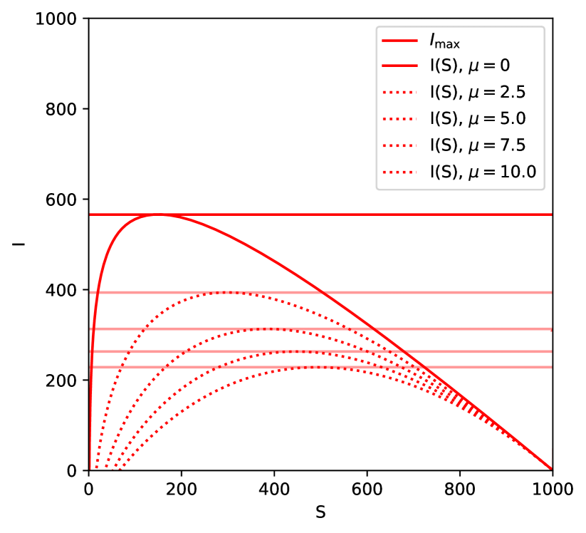
(a) ${I}$ for different parameters $\mu$

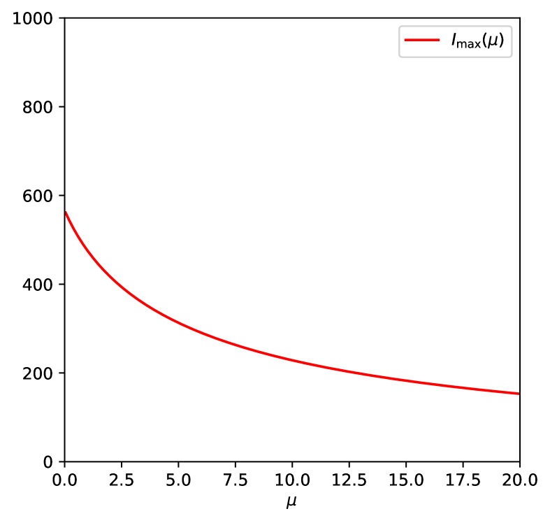
(b) ${I}_{\max}$ of $\mu$

Figure 10. ODE simulations for SIRD model with simple saturation response $\iota({\mathrm{I}};\mu)=\frac{\iota_{0}}{1+\mu{\mathrm{I}}}$, $\iota_{0}=\iota^{0}=0.2$, $\rho=\rho^{0}=0.02$, $\delta=\delta^{0}=0.01$ for different $\mu$.

3.5. Hospitalisation

The SIR model can be extended to include realistic details for the description of the pandemic. One crucial aspect is the presence of a National Health System able to take care of the infected people and in particular of those who need intensive care. In this section, we assume that all infected individuals require hospitalisation. We introduce an additional sub-type for the infected individuals to distinguish between hospitalised and non-hospitalised infected individuals. This results in the types listed in Table 4.

Table 4. The types of the standard SIR model with hospitalisation.

Type	Interpretation
$S$	Susceptible individuals
$I_{h},h\in\{0,1\}$	Infected individuals of hospitalisation class $h$
	$h=1$: hospitalised, $h=0$: not
$R$	Recovered individuals
$D$	Deceased individuals

For $h\in\{0,1\}$ and reaction constants $\iota_{h},\rho_{h},\delta_{h}>0$, we consider the following rules describe type changes:

$$S+I_{h} $\displaystyle\xrightarrow{\iota_{h}}$\hfil\ignorespaces I_{0}+I_{h},$$ [Infection] (3.25)

$$I_{0} $\displaystyle\xrightarrow{\eta(I_{1})}$\hfil\ignorespaces I_{1},$$ [Hospitalisation]

$$I_{h} $\displaystyle\xrightarrow{\rho_{h}}$\hfil\ignorespaces R,$$ [Recovery]

$$I_{h} $\displaystyle\xrightarrow{\delta_{h}}$\hfil\ignorespaces D,$$ [Death]

Here, $\eta(I_{1})$ denotes the hospitalisation rate which depends on the number of hospitalised individuals $I_{1}$. We choose $\eta(I_{1})=\eta_{0}\frac{H_{\max}-I_{1}}{N}$, where $\eta_{0}>0$ and $0<H_{\max}\leq N$ denotes the (known) maximum capacity of hospitalisation, i.e. $H_{\max}$ is the maximum number of available hospital beds. We assume $\rho_{0}<\rho_{1}$ and $\delta_{0}>\delta_{1}$ because recovery in hospital is more likely and death is less probable due to the assumption that hospitalisation is put up on infected individuals regardless of the severity. We also suppose that $\iota_{1}<\iota_{0}$ as new infections are reduced by controlling inside hospitals. The rules above can be associated with the following propensities and lead to a system of ordinary differential equations:

Propensities with numbers:

$$\kappa_{1}({S},{I}_{0},{I}_{1},{R},{D}) =\frac{\iota_{0}}{N}{S}{I}_{0},$$ (3.26)

$$\kappa_{2}({S},{I}_{0},{I}_{1},{R},{D}) =\frac{\iota_{1}}{N}{S}{I}_{1},$$

$$\kappa_{3}({S},{I}_{0},{I}_{1},{R},{D}) =\eta({I}_{1}){I}_{0},$$

$$\kappa_{4}({S},{I}_{0},{I}_{1},{R},{D}) =\rho_{0}{I}_{0},$$

$$\kappa_{5}({S},{I}_{0},{I}_{1},{R},{D}) =\rho_{1}{I}_{1},$$

$$\kappa_{6}({S},{I}_{0},{I}_{1},{R},{D}) =\delta_{0}{I}_{0},$$

$$\kappa_{7}({S},{I}_{0},{I}_{1},{R},{D}) =\delta_{1}{I}_{1}.$$

ODEs with fractions:

$$\frac{\mathop{}\!\mathrm{d}{\mathrm{S}}}{\mathop{}\!\mathrm{d}t} =-(\iota_{0}{\mathrm{I}}_{0}+\iota_{1}{\mathrm{I}}_{1}){\mathrm{S}},$$

$$\frac{\mathop{}\!\mathrm{d}{\mathrm{I}}_{0}}{\mathop{}\!\mathrm{d}t} =(\iota_{0}{\mathrm{I}}_{0}+\iota_{1}{\mathrm{I}}_{1}){\mathrm{S}}-(\rho_{0}+\delta_{0}){\mathrm{I}}_{0}-\eta({\mathrm{I}}_{1}){\mathrm{I}}_{0},$$

$$\frac{\mathop{}\!\mathrm{d}{\mathrm{I}}_{1}}{\mathop{}\!\mathrm{d}t} =-(\rho_{1}+\delta_{1}){\mathrm{I}}_{1}+\eta({\mathrm{I}}_{1})){\mathrm{I}}_{0},$$ (3.27)

$$\frac{\mathop{}\!\mathrm{d}{\mathrm{R}}}{\mathop{}\!\mathrm{d}t} =\rho_{0}{\mathrm{I}}_{0}+\rho_{1}{\mathrm{I}}_{1},$$

$$\frac{\mathop{}\!\mathrm{d}{\mathrm{D}}}{\mathop{}\!\mathrm{d}t} =\delta_{0}{\mathrm{I}}_{0}+\delta_{1}{\mathrm{I}}_{1}.$$

At the infection free steady state $(1,0,0,0,0)$, the right-hand side of (3.5) can be linearised as

$$\begin{pmatrix}0&-\iota_{0}&-\iota_{1}&0&0\cr 0&\iota_{0}-\rho_{0}-\delta_{0}-\eta(0)&+\iota_{1}&0&0\cr 0&\eta(0)&-\rho_{1}-\delta_{1}&0&0\cr 0&\rho_{0}&\rho_{1}&0&0\cr 0&\delta_{0}&\delta_{1}&0&0\end{pmatrix}.$$

The eigenvalues of the linearisation are given by the zeros of

$$P(z)=-{{z}^{3}}[\left(\iota_{0}-\eta(0)-z-\rho_{0}-\delta_{0}\right)\left(-z-\rho_{1}-\delta_{1}\right)-\iota_{1}\eta(0)].$$ (3.28)

There are three zero eigenvalues and for large $\eta(0)$ the equation reduces to:

$$z^{2}+\eta(0)\,z+(\rho_{1}+\delta_{1}-\iota_{1})\eta(0)=0$$

which has negative eigenvalues for $\iota_{1}<\rho_{1}+\delta_{1}$. For large $\eta(0)$ the infection free state has two asymptotically stable directions if in hospital the rate of infection is smaller than the sum of death and recovery rate.

To compute $R_{0}$ we use the construction due to Diekmann in [19] for

$$\left.\begin{pmatrix}\frac{\mathop{}\!\mathrm{d}{\mathrm{I}}_{0}}{\mathop{}\!\mathrm{d}t}\\ \frac{\mathop{}\!\mathrm{d}{\mathrm{I}}_{1}}{\mathop{}\!\mathrm{d}t}\end{pmatrix}\right|_{\text{DFE}}=\begin{pmatrix}\iota_{0}-(\rho_{0}+\delta_{0}+\eta(0))&\iota_{1}\\ \eta(0)&-(\rho_{1}+\delta_{1})\end{pmatrix}\begin{pmatrix}{\mathrm{I}}_{0}\\ {\mathrm{I}}_{1}\end{pmatrix}$$

and split this Jacobian into transmission $T$ and transition $\Sigma$, yielding for NGM with large domain (using notation and definition in [19]):

$$T =\begin{pmatrix}\iota_{0}&\iota_{1}\\ 0&0\end{pmatrix},\quad\Sigma=\begin{pmatrix}-(\rho_{0}+\delta_{0}+\eta(0))&0\\ \eta(0)&-(\rho_{1}+\delta_{1})\end{pmatrix}$$

$$K_{L} =-T\Sigma^{-1}=\begin{pmatrix}\frac{\iota_{0}}{\rho_{0}+\delta_{0}+\eta(0)}+\frac{\eta(0)}{\rho_{0}+\delta_{0}+\eta(0)}\cdot\frac{\iota_{1}}{\rho_{1}+\delta_{1}}&\frac{\iota_{1}}{\rho_{1}+\delta_{1}}\\ 0&0\end{pmatrix}.$$

The NGMs $K$ and $K_{L}$ have the same spectral radius (see [19]), thus

$$R_{0}=\frac{\iota_{0}}{\rho_{0}+\delta_{0}+\eta(0)}+\frac{\eta(0)}{\rho_{0}+\delta_{0}+\eta(0)}\cdot\frac{\iota_{1}}{\rho_{1}+\delta_{1}}.$$

Note that the initial hospitalisation rate $\eta(0)$ can contribute to stability and to keep $R_{0}<1$ and also that for zero capacity $\eta(0)=0$ we retain the basis reproduction number of the standard SIRD model. For large $\eta(0)$ the value of $R_{0}$ is determined by $\iota_{1}/(\rho_{1}+\delta_{1})$ and hence $R_{0}<1$ for $\iota_{1}<\rho_{1}+\delta_{1}$. In terms of stability of the disease-free equilibrium this coincide with the study of the spectrum of the linearisation of the vector field (for a proof, see [66]).

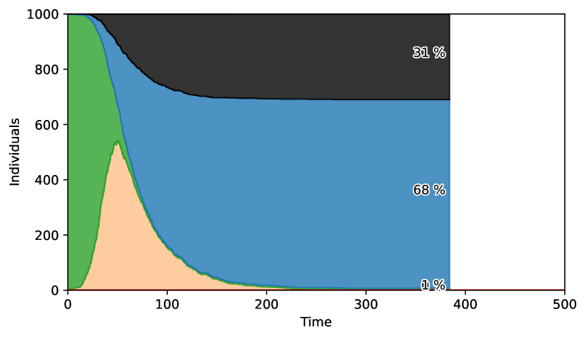
(a) $H_{\max}=0$

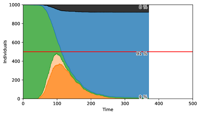
(b) $H_{\max}=500$

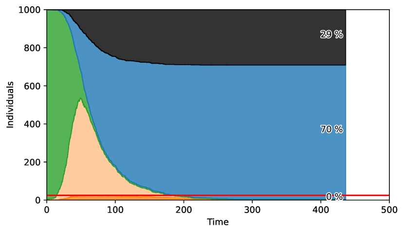
(c) $H_{\max}=25$

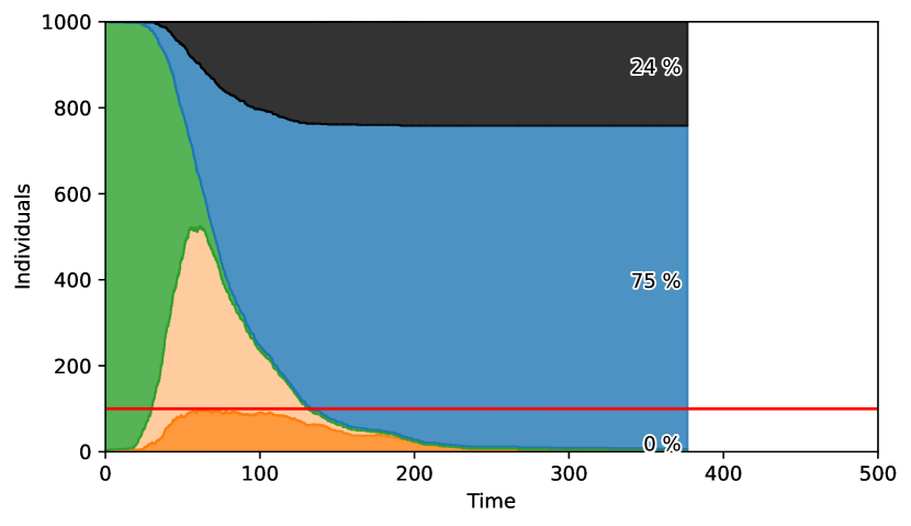
(d) $H_{\max}=100$

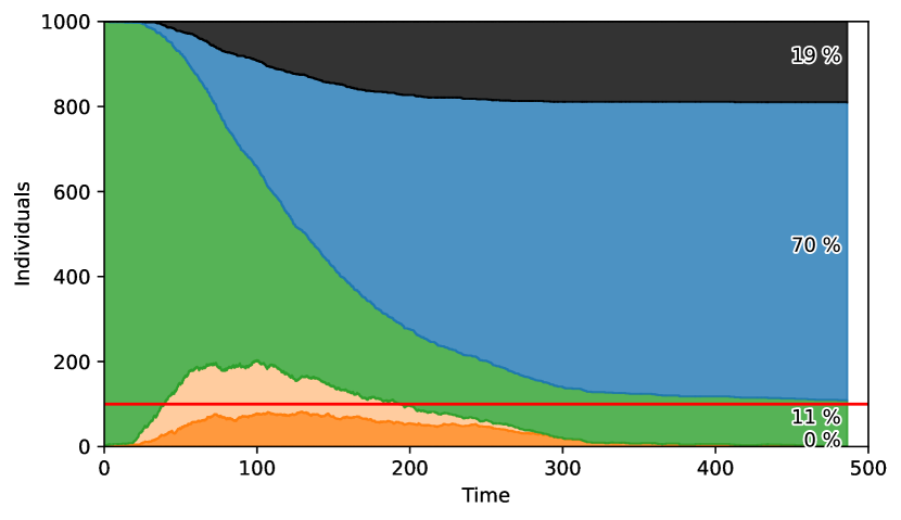
(e) $H_{\max}=100$, $\lambda=10$, $\vartheta=\frac{{I}_{0}+{I}_{1}}{N}$

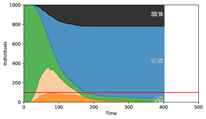
(f) $H_{\max}=100$, $\lambda=1$, $\vartheta=\frac{{I}_{1}}{H_{\max}}$

Figure 11. SSA simulations for SIRD model with hospitalisation for different health care capacities. For 11(e) and 11(f) including responses $f(\vartheta;\lambda)=\frac{1}{1+\lambda\vartheta}$ for $\iota(\vartheta,\lambda)=\iota\cdot f(\vartheta,\lambda)$, based on different information $\vartheta$. $\iota=\iota^{0}(1.,0.5)$, $\rho=\rho^{0}(1,1.2)$, $\delta=\delta^{0}(1.,0.1)$, $\eta_{0}=0.6$.

Figure 11 shows the effect of the health system in particular in reducing the number of fatalities. Without any hospitalisation capacity in Figure 11(a) the course of the epidemic is exactly the same as the standard case. If the capacity is very large as in Figure 11(b), almost every infected can be treated and thus the fraction of deceased is very low. Figures 11(c) and 11(d) show that for an overwhelmed health care system the fatalities are almost as high as without. For the simulations in Figures 11(e) and 11(f) we also included functional responses for the infection rate $\iota f(\vartheta)$, effectively reducing contacts, see Section 3.4, to emphasise the effect of flattening-the-curve on the total number of deceased individuals. There we can read the combined effect of retarding infection cases by behaviour, usually called flattening-the-curve, and the thus well functioning hospitalisation, reducing the proportion of deceased. In Figure 11(e) the response is proportional to the fraction of all infected $\frac{I_{0}+I_{1}}{N}$. In contrast to the difficulty to measure the number of infected individuals (Figure 11(e)) the dependence on information for Figure 11(f) is based on the easy to obtain occupancy of the hospitals $\frac{I_{1}}{H_{\max}}$. As $N=10\cdot H_{\max}$ the behaviour would be much more sensitive on the fraction of hospitalised, therefore we rescaled the behavioural parameter to $\lambda=1$. We observe a less effective flattening-the-curve with larger death fraction (21% vs 16%) as $I_{0}$ has no influence.

3.6. Lockdowns And Other Policies

A common measure used to reduce the spread of an epidemic is lockdowns. In which, in contrast to individual behavior, a reduction in contact is imposed on the entire population for a certain period of time. We model a single lockdown by a nonnegative piecewise constant function $\iota(t)$ for the infection rate in the rules (3.1) and (3.2):

$$\iota(t)=\begin{cases}\iota_{0}\cdot(1-\lambda_{s})&\text{for }T_{s}\leq t<T_{e},\\ \iota_{0}&\text{else},\end{cases}$$ (3.29)

where $\iota_{0}>0$ is the infection rate without lockdown and $0\leq T_{s}<T_{e}\leq T$ denote the start and end time, respectively. Further, $\lambda_{s}\in[0,1)$ is the severity of the reduction in contact. This function can be easily generalized to multiple lockdowns with start and end times as well as severity depending on global information like, e.g. incidence or effective reproduction number. For a model with lockdown based on imposed change of behaviour, see Figure 19.

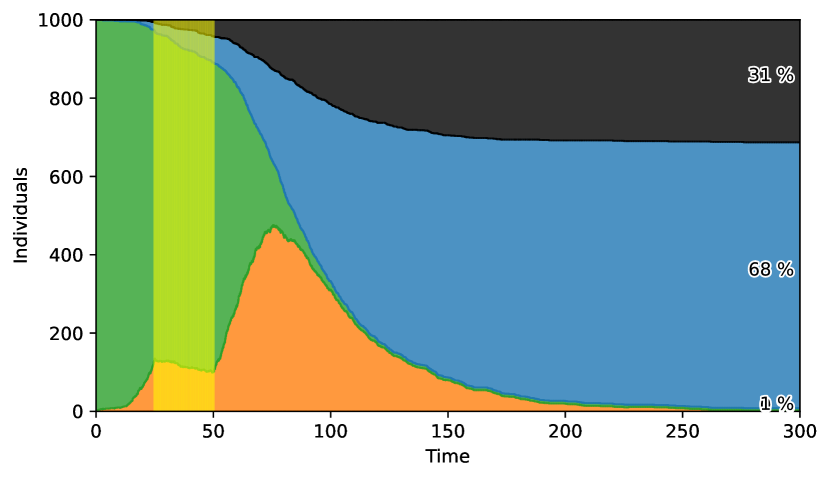
(a) short, but strict: $T_{s}=25$ to $T_{e}=50$, contact reduction of $\lambda_{s}=0.9$

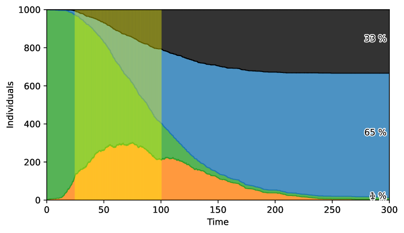
(b) long, but less strict: $T_{s}=25$ to $T_{e}=100$, contact reduction of $\lambda_{s}=0.6$

Figure 12. SSA simulation for SIRD model with lockdowns of different duration and contact reduction. $\iota_{0}=\iota^{0}=0.2$, $\rho=\rho^{0}=0.02$, $\delta=\delta^{0}=0.01$. Duration and severeness of lockdown in yellow.

In Figure 4 we observe how lockdown duration and severity affects the trajectories for number of infected individuals. The beginning of lockdown is for both simulations at an early stage of exponential growth. In Figure 12(a) a very strict but short lockdown reduces the number of infected. However after the restrictions the number raises almost to the same peak as without lockdown due to the high number of susceptibles. Whereas for a long but less strict lockdown, the number of infected still increases with a lower slope. That enables infectious individuals changing to recovered or deceased state, thus effectively reducing the number of susceptibles. Therefore, after the lockdown the number of infected raises only marginally. Both simulations result in almost the same shares for final size. In reality flattening the curve, by e.g. lockdowns as in Figure 12(b), is important to avoid break down of health care systems. Otherwise this would lead to higher number of deceased individuals, see also Section 3.5 and Figure 11.

3.7. Immunity

The immunity status of individuals plays of course a major role in the COVID-19 pandemic. Initially, as this coronavirus did not previously spread in human populations, there was nearly no adaptive immunity present before the COVID-19 pandemic. Humans have already some base innate immunity which defends the body in an unspecific way, also against a coronavirus. But so-called adaptive immunity will be much more important, and we discuss only this kind of defence against pathogens. A low level of adaptive immunity might be present from previous infections with a different kind of coronavirus. Adaptive immunity levels will be proportional to the level of lymphocytes remembering a SARS-CoV-2 infection or corresponding vaccination, and can be measured. Adaptive immunity can depend on genetic variability, but also on the health status of an individual, and other variables, such as surely age. For example, certain Neanderthal genes present in an individual can either severely increase or reduce the risk of a COVID-19 infection [74], [73]. Environmental factors can also not be excluded to change individual immunity.

Adaptive immunity in animals and therefore humans therefore strongly depends on what is called immunological memory created by the adaptive immune response. This memory can be trained to detect different very specific molecules or molecule parts which do not normally belong to a body. This training is done by infections, but also vaccinations. For mathematical models of COVID-19 it is essential to project the immunological memory into an ordered space, because a better immunological memory for a certain pathogen should imply better immunity. Conversely, immunological memory can also deteriorate over time, and therefore immunity against some pathogen will decline as well. In an individually structured model immunity against SARS-CoV-2 could likely be modelled by a scalar ordinary differential equation on $\mathbb{R}_{0}^{+}$, with $0$ having the interpretation of no immunity, and more positive values interpreted as having acquired more immunity. Let $I\in\mathbb{R}_{0}^{+}$ denote this immunity level of an individual since the last infection or vaccination event occurring at time $t_{0}$. Here we use the same symbol as for the type of infected/ infectious individuals as we consider only immune response to an infection, for vaccination type $S$ for susceptible is more appropriate. Let $A\in\mathbb{R}_{0}^{+}$ be the age of the individual, and $H\in\mathbb{R}_{0}^{+}$ be another parameter, a one-dimensional projection of the health status of an individual. Let $G\in\mathbb{R}_{0}^{+}$ be yet another parameter, a one-dimensional projection of the gene set of an individual, as a risk factor for COVID-19 infections. Then we could assume

$$\begin{split}&\frac{dI}{dt}=f(A,H,G;I),\\ &I(t_{0})=I_{0}.\\ \end{split}$$ (3.30)

Here, we assume as well that no secondary infection or vaccination occurred during the time-course of the immunological response given by (3.30). We assume deterministic dynamics in an individual, because the various immune responses in the body are based on a large number of biochemical molecular interactions. Using a law-of-large-numbers argument then justifies the deterministic assumption. Given the data we have on immunological responses, the solution of (3.30) should give us an immunological response curve as exemplary given in Figure 13, top. Initially, the level of immunity will have to built up, reaching maximal protection against the coronavirus at some time $\bar{t}>t_{0}$. After the maximum has been reached, the immune system for efficiency reasons will have to slowly reduce immunity levels.

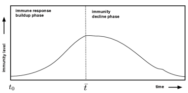
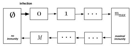
Figure 13. Top: typical time course of immunity levels after infection, no time scales given. In an initial phase after infection immunity builds up to a maximal level, afterwards immunity levels are declining again, eventually reaching full susceptibility again. Bottom: In a framework model immunity levels are discreet. Transition rates $\varphi$ in equation (3.31) model how individuals in a certain immunity class transition between levels.

As we do not have considered individual-based models in our framework, we will have to mimic the modelling idea from the ODE (3.30). Our classification scheme only allows a finite discrete number of immunity types. Let $M+1\in\mathbb{N}$ be the number of types we are using, with $0$ included as the first index. The immunity types are not describing immunity levels, i.e. how well an immune system can fight a virus infection. As discussed, immunity levels should qualitatively follow the time course given in Figure 3.31, top. If we mimic this immunity level time course on a discrete level, then there will be an index $0<m_{\text{max}}<M$ where maximal immunity will be achieved, see Figure 3.31, bottom. Note that in model (3.31) immunity levels are not included, only the transition through the immunity types is described. If an infection process is introduced on top of this model, we will of course have to introduce immunity levels. We leave this modelling to later publications.

$$\emptyset $\displaystyle\xrightarrow{\iota}$\hfil\ignorespaces I_{0}$$ [Immunity Level after (3.31)

Infection / Vaccination]

$$I_{m} $\displaystyle\xrightarrow{\varphi_{m}}$\hfil\ignorespaces I_{m+1}, \quad m=0,\ldots,M-1$$ [Changing Immunity Level]

$$I_{M} $\displaystyle\xrightarrow{\varphi_{M}}$\hfil\ignorespaces \emptyset$$ [Final Loss of Immunity]

Here $\iota>0$ denotes the infection rate and the differently indexed $\varphi_{m}>0$ are immunity transition rates determined by immunity profiles as sequences $p=\{(d_{m},i_{m})\}_{m\in\{0,\ldots,M\}}$ describing the level of immunity $i_{m}$ spend for the time interval $d_{m}$ in immunity class $I_{m}$. Note that for this model the immunity values $i_{m}$ are not used, but for the next model based on infectivity.

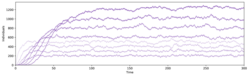
(a) Number of individuals in immunity levels over time.

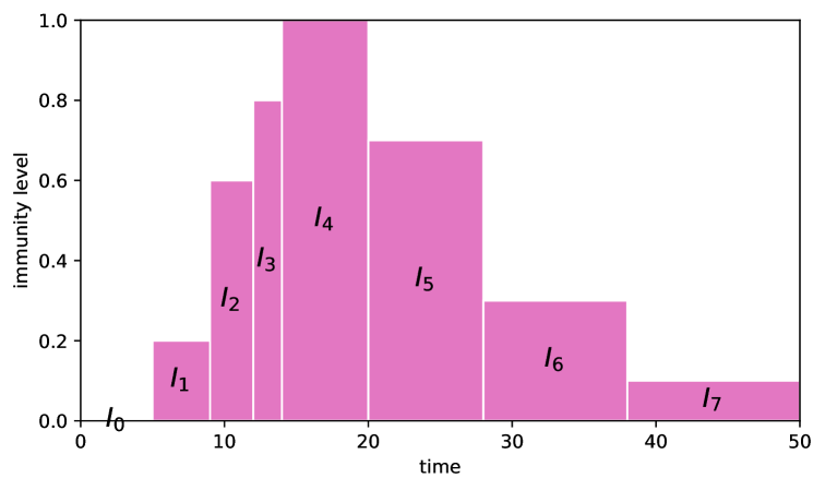
(b) Individual immunity profile.

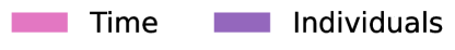
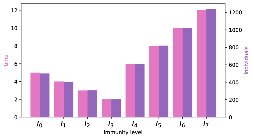
(c) Time spent resp. mean over $[0.5T,T]$ of individuals in immunity classes.

Figure 14. SSA simulation for immunity model with individual profile and over second half of time interval averaged numbers of individuals in different classes. $\iota=100$, $\varphi_{m}=\frac{1}{d_{m}}$.

Also for the simulation in Figure 14 we restrict to immunity progressing. With rate $\iota$ we introduce a constant influx of infected individuals. Infected individuals pass a complex immunity progressing profile, see Figure 14(b), and finally leave the system. In Figure 14(a) we observe that after a certain time the numbers of individuals in immunity classes stabilise, reproducing the lengths of the time intervals spent in different immunity classes of the individual profile, see Figure 14(c).

3.8. Infectivity

Infectivity can be almost identically discussed to immunity from a mathematical modelling point-of-view. The major difference is that infectivity levels of an individual now will be proportional to internal virus production after an infection, and not the level of individual immunity, which possibly can change on different time scales. But the basic increase of infectivity after infection, and then a reduction of virus levels after an efficient immune response, will still be present. We therefore get a qualitative description of infectivity levels like in Figure 13. Therefore we as well denote infectivity classes by $I_{m}$, treating the levels as sub-types of infected $I$ in a classification scheme, see Table 5 together with types describing the infection process. To link infectivity and the standard SIRD model in the following rules (3.32), we use infectivity profiles as sequences $p=\{(d_{m},i_{m})\}_{m\in\{0,\ldots,M\}}$ describing the level of infectivity $i_{m}$ spend for the time interval $d_{m}$ in infectivity class $I_{m}$. The infection rates $\iota_{m}=\iota^{0}c_{I}i_{m}$ and the death rates $\delta_{m}=\delta^{0}c_{I}i_{m}$ are proportional to the infectivity levels, whereas the transition rates $\varphi_{m}=c_{D}\frac{1}{d_{m}}$ are inversely proportional to the time intervals.

Table 5. The types of the standard SIR model with different infectivity classes.

Type	Interpretation
$m\in\{0,\ldots,M\}$	index for Sub-type	of infectivity class
$S$	Susceptible individuals
$I_{m}$	Infectious individuals	of infectivity class $m$
$R$	Recovered individuals
$D$	Deceased individuals

$$S+I_{m} $\displaystyle\xrightarrow{\iota_{m}}$\hfil\ignorespaces I_{0}+I_{m}, \quad 0 \leq m\leq M,\quad$$ [Infection] (3.32)

$$I_{m} $\displaystyle\xrightarrow{\varphi_{m}}$\hfil\ignorespaces I_{m+1}, \quad 0 \leq m\leq M-1,\quad$$ [Changing Infectivity]

$$I_{M} $\displaystyle\xrightarrow{\varphi_{M}}$\hfil\ignorespaces R,$$ [Loss of Infectivity / Recovery]

$$I_{m} $\displaystyle\xrightarrow{\delta_{m}}$\hfil\ignorespaces D, \quad 0 \leq m\leq M.\quad$$ [Death]

Propensities with numbers:

$$\kappa_{1}({S},{I},{R},{D}) =-\sum_{0\leq m\leq M}\frac{\iota_{m}}{N}{I}_{m}{S},$$

$$\kappa_{2,m}({S},{I},{R},{D}) =\varphi_{m}{I}_{m},\enspace 0\leq m\leq M-1,$$

$$\kappa_{3}({S},{I},{R},{D}) =\varphi_{M}{I}_{M},$$ (3.33)

$$\kappa_{4,m}({S},{I},{R},{D}) =\delta_{m}{I}_{m},\enspace 0\leq m\leq M,$$

ODEs with fractions:

$$\frac{\mathop{}\!\mathrm{d}{\mathrm{S}}}{\mathop{}\!\mathrm{d}t} =-{\mathrm{S}}\sum_{0\leq m\leq M}\iota_{m}{\mathrm{I}}_{m},$$

$$\frac{\mathop{}\!\mathrm{d}{\mathrm{I}}_{0}}{\mathop{}\!\mathrm{d}t} ={\mathrm{S}}\sum_{0\leq m\leq M}\iota_{m}{\mathrm{I}}_{m}-(\varphi_{0}+\delta_{0}){\mathrm{I}}_{0},$$

$$\frac{\mathop{}\!\mathrm{d}{\mathrm{I}}_{m}}{\mathop{}\!\mathrm{d}t} =\varphi_{m-1}{\mathrm{I}}_{m-1}-(\varphi_{m}+\delta_{m}){\mathrm{I}}_{m},\enspace 1\leq m\leq M,$$

$$\frac{\mathop{}\!\mathrm{d}{\mathrm{R}}}{\mathop{}\!\mathrm{d}t} =\varphi_{M}{\mathrm{I}}_{M},$$ (3.34)

$$\frac{\mathop{}\!\mathrm{d}{\mathrm{D}}}{\mathop{}\!\mathrm{d}t} =\sum_{0\leq m\leq M}\delta_{m}{\mathrm{I}}_{m},$$

infectivity profiles

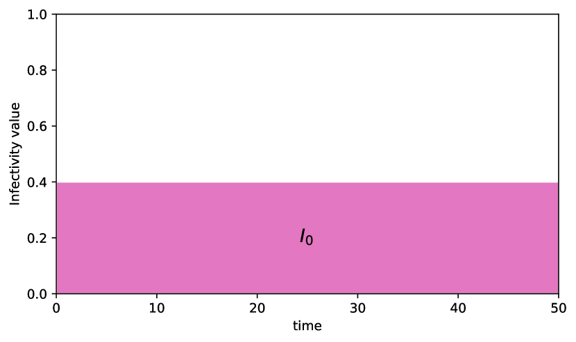
(a) single infectivity class

epidemic over time

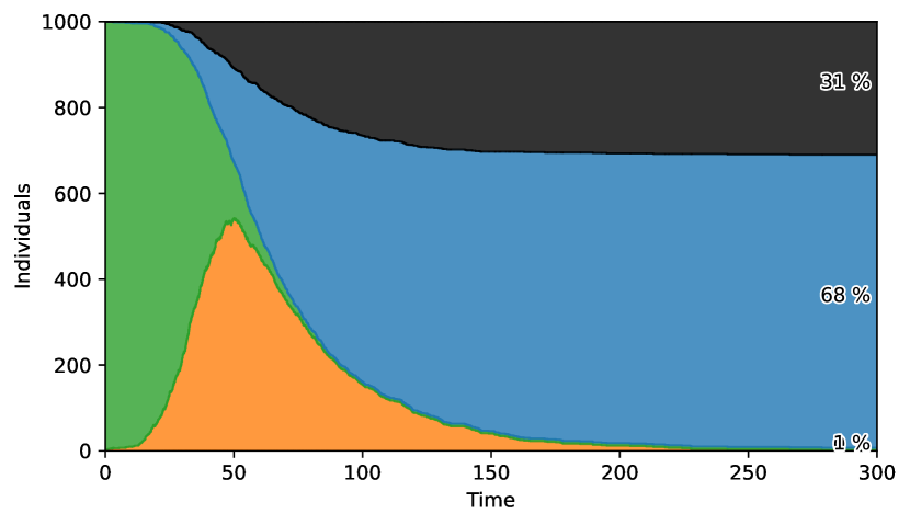
(b) single infectivity class

(c) two classes, SEIRD

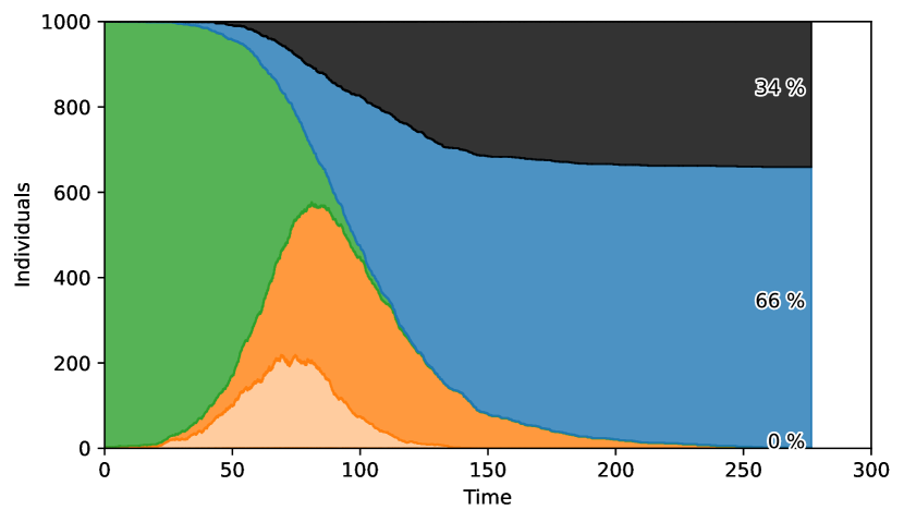
(d) two classes, SEIRD

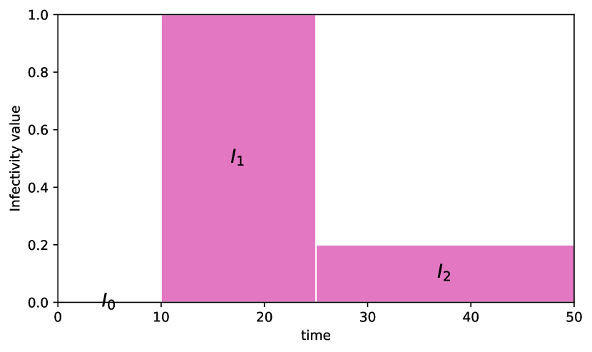
(e) three classes

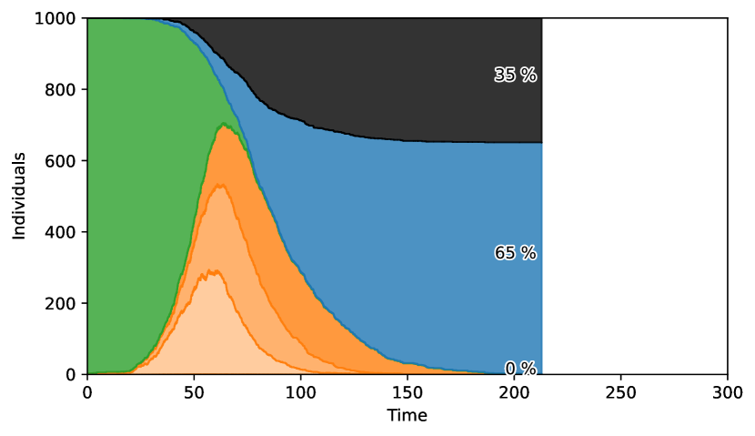
(f) three classes

Figure 15. Infectivity profiles and SSA simulations for SIRD model with infectivity.

infectivity profiles

(a) 8 classes

epidemic over time

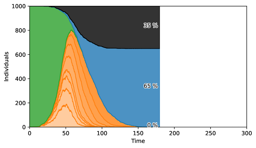
(b) 8 classes

(c) 8 classes, constant infectivity

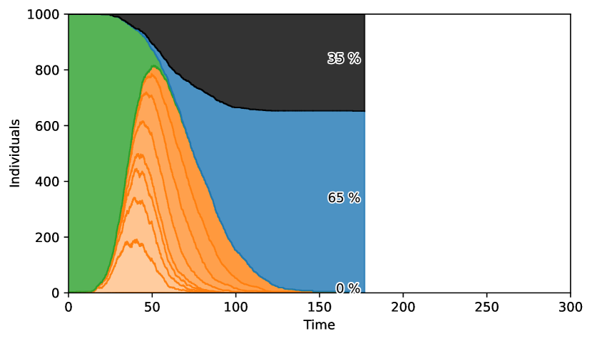
(d) 8 classes, constant infectivity

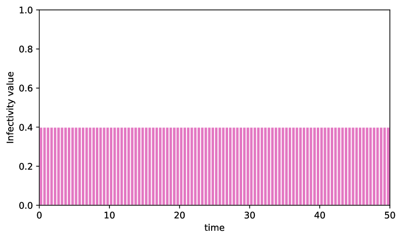
(e) 100 classes, constant infectivity

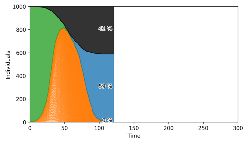
(f) 100 classes, constant infectivity

Figure 16. Finer infectivity profiles and SSA simulations for SIRD model with infectivity.

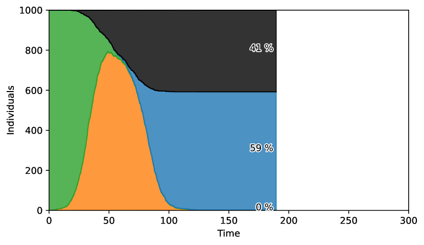
(a) SSA with one infectivity class but discrete delay for recovery.

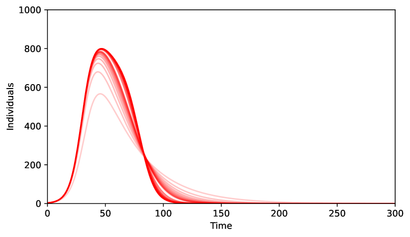
(b) ODE $I$ for increasing number of infectivity classes with constant value.

Figure 17. Single rule with delay as limit and ODE solutions for $I$ for increasing number of infectivity classes.

For the SSA simulations in Figures 15 and 16 all infectivity profiles have same total duration of $50$ and mean infectivity $0.4$. The proportionality constant for infection rates $\iota_{m}=\iota^{0}c_{I}i_{m}$ is set to $c_{I}=2.5$. In Figure 15(b) the single constant profile of Figure 15(a) reproduces the base case. A model equivalent to the SEIRD with the additional type E for exposed can be achieved by introducing for Figure 15(c) an infectivity class, here $I_{0}$, with zero infectivity $i_{0}=0$. This delays the wave of infections. Using more and more infectivity classes results in steeper increase of infected individuals, see Figures 15(f), 16(b), 16(d) and, for $100$ infectivity classes, Figure 16(f). The number of classes influences the maximum number of infected individuals, whereas the infectivity values rather have influence on the time course. Compare Figure 16(a) with Figure 16(c). High numbers $M$ of infectivity classes approximate the case for only one infectivity class but discrete delay due to the remaining sum of expected waiting times, but with increasing $M$ decreasing variance, see Figure 16(c) and Figure 6. Also the trajectories of infected individuals for ODE simulations in Figure 17(b) converge. The white gap is due to changing from $M\in\{1,2,\ldots 10\}$ to $M\in\{20,30,\ldots,100\}$. We observe that a solution of a delay equation can be approximated by a solution of a chain of ODEs.

3.9. Behaviour

A striking aspect of the COVID-19 pandemic from the beginning was the difference in people’s behaviour, taking more or less infection risk due to necessities like age vulnerability, social status or professional occupation, but also more free characteristics like lifestyle choices. Of course face mask wearing as a protective measure belongs to this behavioural category, sometimes imposed behaviour, sometimes voluntary. Face mask wearing and social distancing are prime examples for social behaviour relevant for the course of the COVID-19 pandemic. Therefore, given these two examples, we mainly consider behaviour in this Section 3.9 that is based on choice, however embedded and moderated by cultural and economical factors in the society in which an individual lives.

Face mask wearing has become the ‘face’ of the 2020 COVID-19 pandemic, and will surely stay as a behavioural change, for example in European countries, in the years to come. Face mask wearing is surprisingly effective, see [23] for a list of different studies. However, like vaccination, face mask wearing has been subject to political discussions and identity politics [60]. This example also shows how important opinion formation games are with respect to understanding something like a COVID-19 pandemic.

To model behaviour on top of an epidemic process we introduce an index set $B:=\{1,\ldots,n_{B}\}$, indexing linearly ordered classes of behaviour, with larger indices indicating higher infection risk and vice versa. The associated types are listed in Table 6. The interpretation is that different sets of behaviour of individuals lead to a certain behavioural profile, to which we can assign a certain objective risk level. For example, considering face mask wearing, the value $n_{B}$ could describe individuals never wearing a face mask, and $1$ models individuals always wearing a face mask, with $b\in B\backslash\{1,n_{B}\}$ describing different forms of more moderate face mask wearing behaviour. In practice, this empirical connection will be hard to establish in some cases, but on the other hand, different behavioural risk levels clearly exist.

Table 6. The types of the adapted COVID-19 behavioural class structured SIRD model.

Types	Interpretation
$S_{b},b\in B$	Susceptible individuals	of behavioural class $b$
$I_{b},b\in B$	Infectious individuals	of behavioural class $b$
$R_{b},b\in B$	Recovered individuals	of behavioural class $b$
$D_{b},b\in B$	Individuals that have died

For reaction constants $\iota_{b,b^{\prime}},\rho_{b,b^{\prime}},\delta_{b}$, $b,b^{\prime}\in B$, the following rules describe type changes:

$$S_{b}+I_{b^{\prime}} $\displaystyle\xrightarrow{\iota_{b, b'}}$\hfil\ignorespaces \ I_{b}+I_{b^{\prime}}, \quad b,b^{\prime} \in B$$ [Infections] (3.35)

$$I_{b} $\displaystyle\xrightarrow{\rho_{b, b'}}$\hfil\ignorespaces \ R_{b^{\prime}}, \quad b,b^{\prime} \in B$$ [Recovery ]

$$I_{b} $\displaystyle\xrightarrow{\delta_{b}}$\hfil\ignorespaces \ D_{b}, \quad b \in B$$ [Death]

Here, the infectious rates $\iota_{b,b^{\prime}}$ control the rate of spread, i.e. $\iota_{b,b^{\prime}}$ represents the probability of transmitting the disease between a susceptible of behavioural class $b$ and an infectious individual of class $b^{\prime}$. The recovery rates $\rho_{b,b^{\prime}}=1/\tau_{b,b^{\prime}}$ are determined by the average durations $\tau_{b,b^{\prime}}$ of the infection including change of behaviour from class $b$ to $b^{\prime}$ as the recovery process in contrast to the infection is perceived consciously. Modelling choice, we must in addition add further switching behaviour with positive rates $\sigma_{b,b^{\prime}}^{S}$, $\sigma_{b,b^{\prime}}^{I}$ and $\sigma_{b,b^{\prime}}^{R}$ in cases where this is supported by data:

$$S_{b} \xrightarrow{\sigma_{b,b^{\prime}}^{S}} \ S_{b^{\prime}}, \quad b,b^{\prime} \in B,b\neq b^{\prime}$$ [Susceptible Switching] (3.36)

$$I_{b} \xrightarrow{\sigma_{b,b^{\prime}}^{I}} \ I_{b^{\prime}}, \quad b,b^{\prime} \in B,b\neq b^{\prime}$$ [Infected Switching]

$$R_{b} \xrightarrow{\sigma_{b,b^{\prime}}^{R}} \ R_{b^{\prime}}, \quad b,b^{\prime} \in B,b\neq b^{\prime}$$ [Recovered Switching]

The interpretation of introducing switching behaviour is a change of behaviour of an individual. This can be given by information, people watch the news and know, for example, infection numbers are rising rapidly, therefore the own risk increases as well. In this case the switching rate would depend on introducing global information, see Section 2.1.1. But note, in contrast to Section 3.4, which is modelled on basis of the ‘flattening the curve’ ’implicit’ reasoning, where global information influences infectivity rates directly, here behaviour, rules (3.35), and change of behavior, rules (3.36), are explicitly modelled. A second possibility is modelling personal information, for example somebody has a relative who died with coronavirus, and now becomes more prudent. Such local, i.e. personal experiences are best modelled with opinion formation models, see Section 3.12.

We assume for the switching rules (3.36) always that $b\neq b^{\prime}$, as we assume real switching. Note that for a physiological internal state such as age, this switching is not possible. Switching behaviour is admitted not only as a possible albeit random choice, but it is in general influenced by global information like number of infected hospitalised individuals and numbers of death. Note that switching behaviour from one class to another can be seen as an alternative model to the influence of global information on pandemic rates, like predominantly the infection rate, see Section 3.4.

All parameters occurring in this behavioural model are clearly depending on the cultural, social and economic background of individuals. Therefore the behavioral model (3.35) with (3.36) can be used to characterise countries, by parametrising the model with data from different countries or cultural backgrounds.

(a) all refusers (risky), no switching

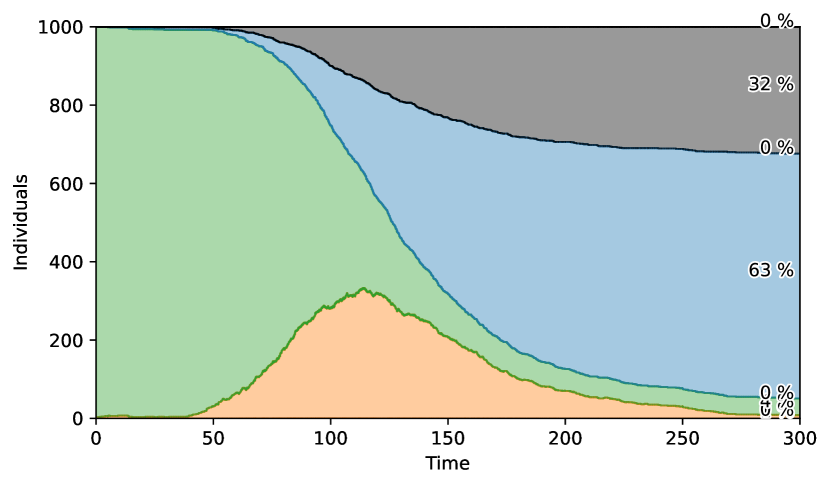
(b) all wearers (wise), no switching

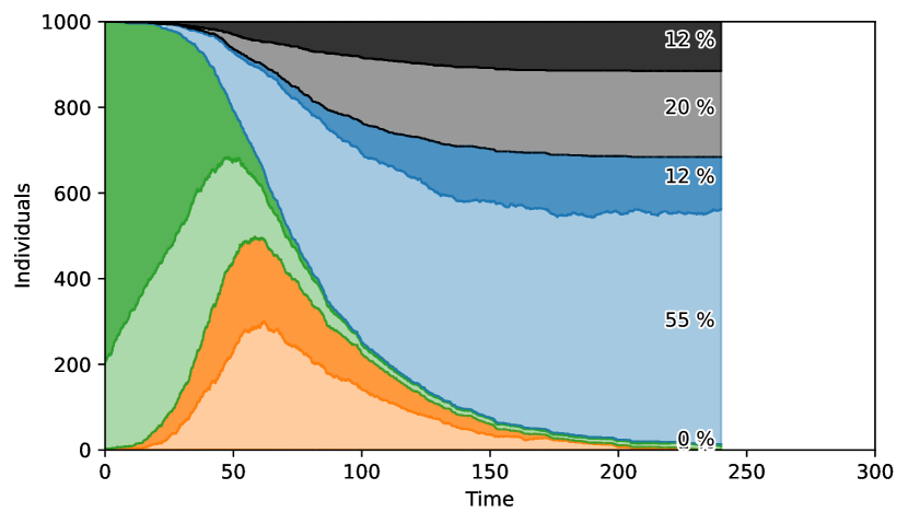
(c) constant switching

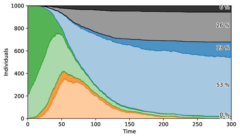
(d) $I$ dependent switching $\sim(1,(1+10\frac{{I}}{N}))$

Figure 18. SSA simulations for SIRD model with behaviour for face mask wearers (wise). ($S_{1},I_{1},R_{1},D_{1}$) and refusers (risky) ($S_{2},I_{2},R_{2},D_{2}$). $\iota=\iota^{0}\left(\begin{smallmatrix}0.5&0.7\\ 0.7&1.0\end{smallmatrix}\right)$, $\rho=\rho^{0}\left(\begin{smallmatrix}1.0&0.0\\ 0.9&0.1\end{smallmatrix}\right)$, $\delta=\delta^{0}(1.,1.)$, $(\sigma_{1,2}^{S},\sigma_{2,1}^{S})=(\sigma_{1,2}^{I},\sigma_{2,1}^{I})=(0.01,0.02)$, $(\sigma_{1,2}^{R},\sigma_{2,1}^{R})=(0.005,0.02)$.

Figure 18 shows SSA simulations for two behavioural groups, i.e. $B=\{1,2\}$. Individuals with $b=2\in B$ refuse wearing face-masks, interpreted as risky behaviour, whereas $b=1$ denotes wise individuals who wear face-masks. The risky behaviour is illustrated in darker colours in Figure 18. For the risky individuals we choose the parameters as for the base case and under the assumption of all individuals are risky and considering the same random seed the simulation results in Figure 18(a) are identical to the ones in Figure 5(a). For the susceptibility and infectivity factors in (3.9) describing the probability of getting infected in (3.9), we assume that for the wise group both values are $70\%$ of the risky group. This reduces the probability of wise-wise infections by approximately $50\%$. The evolution of the epidemic in Figure 18(a) is less steep and has a lower maximum. Recovery and death rates remain unchanged. Both simulations result in almost same final size for deceased individuals, but in Figure 18(a) the amount of susceptibles never got infected is larger. In Figures 18(c) and 18(d) we start with a fraction of $20\%$ wise susceptibles, $3$ risky infectious. The remaining susceptibles individual are risky. By recovery all wise infected stay wise, but the probability of a risky infected remaining risky is only $10\%$; this is a rather optimistic perspective. For Figure 18(c) we choose constant switching rates for risky to wise and vice versa with greater chance of switching to wise than risky. Due to the exponential growth of infectious the constant change of behaviour reduce the maximum of infected only marginally. Whereas in Figure 18(d) with additional increase of all switching rates depending on the fraction of infected, the peak of infected is almost as low as for all wise. In both simulations, the rates $\sigma_{1,2}^{S}$, $\sigma_{1,2}^{I}$, $\sigma_{1,2}^{R}$ govern an inverse transition and are used to model effects related to behaviours related to the lack of trust in scientific results and containment policies that increase the number of individuals who don’t follow the precautions and thus are modeled as constant.

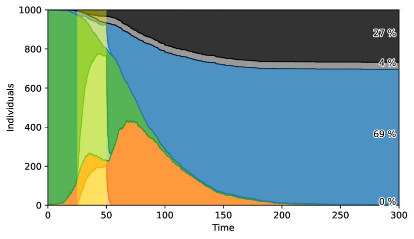
(a) short, but strict, $\lambda_{s}=0.9$, $\sigma=0.1$

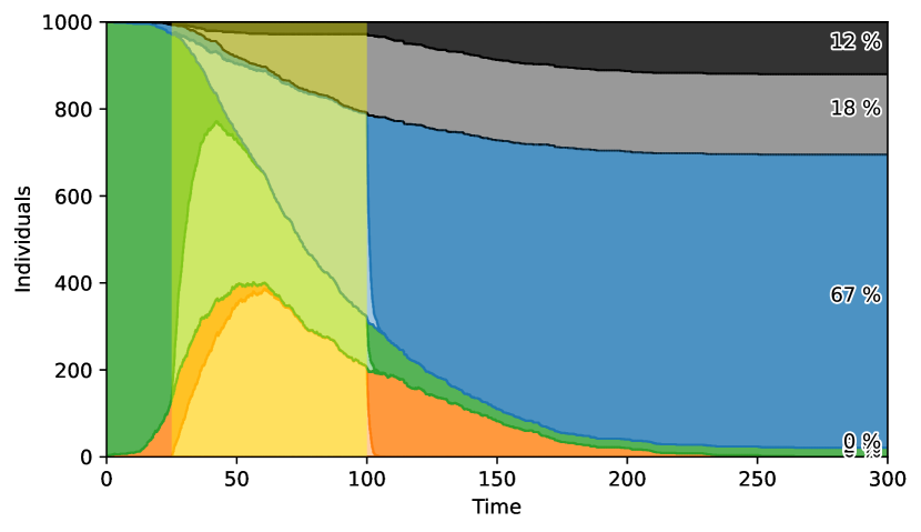
(b) long, but less strict, $\lambda_{s}=0.6$, $\sigma=0.1$

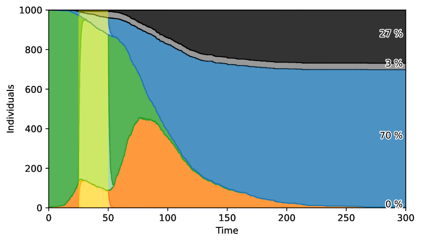
(c) short, but strict, $\lambda_{s}=0.9$, $\sigma=1.0$

(d) long, but less strict, $\lambda_{s}=0.6$, $\sigma=1.0$

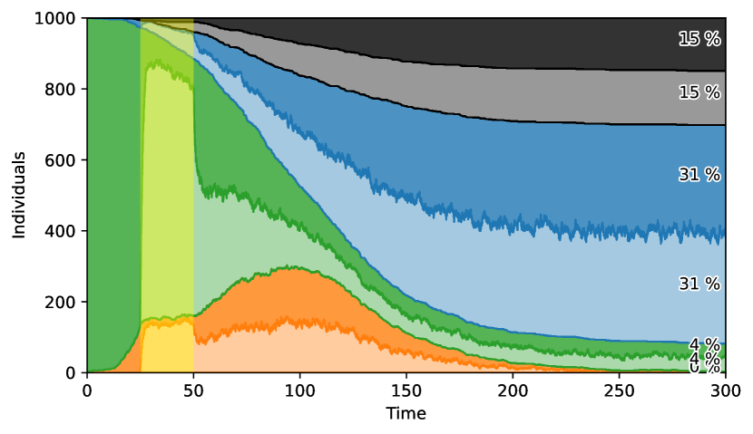
(e) with refusing and remaining behaviour

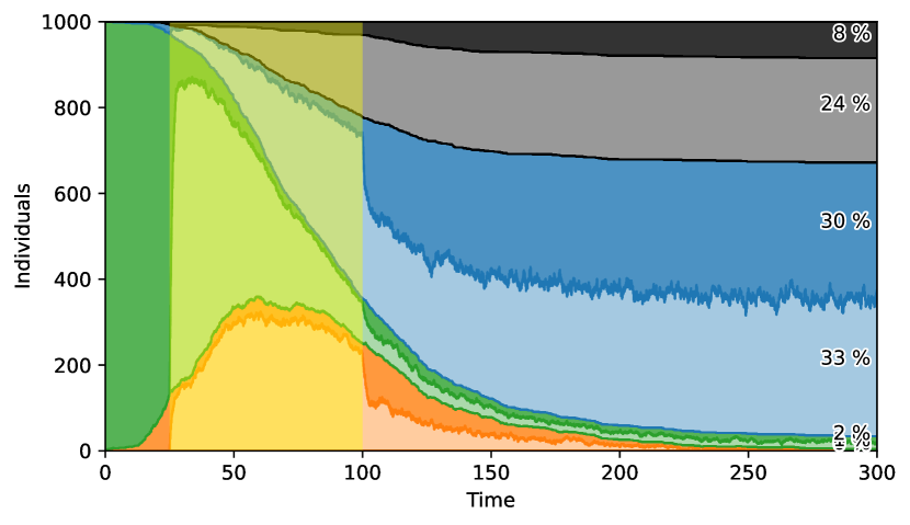
(f) with refusing and remaining behaviour

Figure 19. SSA simulations for SIRD model with lockdown by behaviour. $\iota=\iota^{0}\left(\begin{smallmatrix}1-\lambda_{s}&\sqrt{1-\lambda_{s}}\\ \sqrt{1-\lambda_{s}}&1\end{smallmatrix}\right)$, $\rho=\rho^{0}\left(\begin{smallmatrix}1&0\\ 0&1\end{smallmatrix}\right)$, $\delta=\delta^{0}(1,1)$.

In the SSA simulations in Figure 19 we model lockdowns by imposing behavioural switching in contrast to directly modifying infection parameters as in Figure 4 in Section 3.6. We distinguish between two behavioural groups: $b=2$ for risky individuals with parameters of the base case, and $b=1$ for individuals who decrease their risk of infecting or getting infected by reducing their contacts. We relate the susceptibility $s$ and infectivity $i$ factors, introduced in (3.9) to the severity $\lambda_{s}$ of the lockdowns in Figure 4. For the case $b=1$, we set $s_{1}=i_{1}=\sqrt{(1-\lambda_{s})\iota^{0}}$. The susceptibilty and infectivity factors for the risky group are assumed to be equal and remain $s_{2}=i_{2}=\sqrt{\iota^{0}}$. Thus we get for the matrix of infection rates

$$\iota=\begin{pmatrix}s_{1}\cdot i_{1}&s_{1}\cdot i_{2}\\ s_{2}\cdot i_{1}&s_{2}\cdot i_{2}\end{pmatrix}=\begin{pmatrix}1-\lambda_{s}&\sqrt{1-\lambda_{s}}\\ \sqrt{1-\lambda_{s}}&1\end{pmatrix}\iota^{0}.$$

At the beginning all susceptible individuals are in group with index $b=1$ and disabled switching, i.e. zero rates. In Figures 19(a)-19(d), when lockdown starts at $T_{s}$ – indicated by yellow overlays – individuals are supposed to switch to group $b=2$ with rates $\sigma_{2,1}^{S}=\sigma_{2,1}^{I}=\sigma_{2,1}^{R}=\sigma$, where $\sigma=0.1$ and $\sigma=1.0$, respectively. At the end of lockdown $T_{e}$ individuals switch back again to the group $b=2$ with rates $\sigma_{1,2}^{S}=\sigma_{1,2}^{I}=\sigma_{1,2}^{R}=1.0$. The results, especially for high switching rates, are almost identical to Figures 12(a) and 12(b). Switching with low rates delays the effect of contact reduction. Thus after short and strict lockdowns a high number of infectious and susceptible individuals cause a second wave. For longer but less strict lockdowns almost all infectious reduce their contacts, but not enough and even the nearly constant risky infectious contribute to high number of infected. Whereas high rates only delay minimally the influence of contact reduction and the impact of a too short lockdown dominates. The combination of longer lockdowns and fast switching reduce the peak of infected about $100$. The extend of switching rates imposed by orders may be linked to sociological measure like power distance. In Figures 19(e) and 19(f) we observe that if not all individuals follow the governmental orders, here by a $10\%$ switching rate from wise to risky, the decrease of infected during the lockdown is reduced. If people partly, here with rates $0.5$ from risky to wise and vice versa, maintain their behaviour after lockdown, leads to flatten the curve in Figure 19(e). But in case of remaining behaviour after a longer but less strict lockdown, we only observe a minor contribution.

3.10. Mobility

Mobility is again an important factor in the COVID-19 pandemic dynamics. In fact, it is an important factor in all modern human infectious diseases, due to the enormous increase of mobility in the modern world. At first thought mobility is more connected to multi-compartment models, describing the exchange rates between compartments. In this overview, however, we restrict ourselves to single compartment approaches, leaving multi-compartment models for a later moment. Nevertheless mobility will also effect single compartment models, like those discussed here. How can we incorporate mobility into single-compartment models? There are different ways to do this, and we use mobility to show a different modeling approach within our framework. Instead of sub-classifying the disease states, we classify mobility. Where we assume that the number of individuals is sufficiently large, that the disease state distribution is approximately the same in each sub-class. For mobility we chose the following two-step classification process: First we identify different types of mobility, like short-distance mobility, or long-distance travel etc. We label these types by $M_{1}$ to $M_{m}$, $m\in\mathbb{N}$. The classification is not strict, i.e. individuals can potentially switch mobility classes as we discussed switching behaviour in Section 3.9. The different mobility types are also not ordered, they just describe qualitatively different forms of mobility that can be classified as similar enough (with respect to the pandemic), in order to end up as one type or class. The next step is to introduce sub-types for each mobility class that model the strength or intensity of this kind of mobility. Therefore the intensity sub-types are a strict classification, individuals can be only members of one intensity sub-type. The sub-types are therefore assumed to be linearly ordered, just like immunity (Section 3.7), or infectivity (Section 3.8). We denote the number of intensity sub-types of each mobility class by $l_{1},\ldots,l_{m}$, with $M_{1}^{\alpha},\ldots,M_{m}^{\alpha}$, where the $\alpha$ satisfies $1\leq\alpha\leq l_{i}$, and $i=1,\ldots,m$. As one possibility, we can then interpret mobility as global information, and let the infection process depend on the mobility profile:

$$S+I $\displaystyle\xrightarrow{\iota(M_{1}^{\alpha},\ldots,M_{m}^{\alpha})}$\hfil\ignorespaces 2I$$    [Infections] (3.37)

$$I $\displaystyle\xrightarrow{\rho}$\hfil\ignorespaces R$$    [Recovery]

$$I $\displaystyle\xrightarrow{\delta}$\hfil\ignorespaces D$$    [Death]

Typically, we would assume the infection rate $\iota$ would increase if any of the mobility classes increases in intensity. In the simplest case, with only one mobility class, we model a dependence of the infection rate on just ’mobility’. Instead of mobility classes, we can also consider $M_{1}$ to $M_{m}$ as mobility locations, such as workplaces, parks, retail etc., see Figure 20. This is just another classification scheme, see Section 1.2. Of course we can increase the complexity of rules (3.37) by introducing sub-classes to the disease states, and by making $\rho$ and $\delta$ dependent on mobility, which is implausible from a modelling point-of-view. However, including switching mobility classes as adaptation to the pandemic seems plausible, compare with switching behaviour, i.e. rules (3.36). Due to the assumption of high numbers, simulations for this model would not fit into the family of featured toy models, where $N=1000$. Also ODE simulations are more appropriate.

3.11. Vaccination

The great hope to defeat any transmissible disease is by vaccination. Due to the surprisingly rapid development of COVID-19 vaccines throughout the world, this goal could be in reach for COVID-19. However, there are many obstacles for a successful vaccination strategy to eradicate :

Health, Risk:

Vaccines must prove in clinical trials that their benefits outweigh their health risks. Benefit and risk of a vaccine can depend on individual types, such as age, health status, gender etc.

Economy:

The rate of vaccine production is depending on global supply chains. Vaccine production rates are still too small to enable a global single-event roll-out. Production rates and distribution rates are therefore truly important parameters in realistic epidemiological models. Not every country has vaccine production capabilities, and therefore will have to rely on international efforts of vaccine distribution.

Behaviour, Politics:

Any vaccination strategy must take into account how a population can achieve trust in vaccine reliability, once vaccines are available in sufficient numbers. Risks and benefits of the different available vaccines must be clearly communicated by authorities, in which people have trust.

Vaccine Type, Temporal Vaccination Spacing:

Due to the fact that there are now a number of different vaccines available based on different vaccine methodology, there is a combinatorial problem to be solved which combinations of vaccines in which temporal spacing maximises immunity of individuals. Due to the lack of availability of vaccines, for example, some countries have delayed a second vaccination of the same vaccine to boost the immune system with some success. Trials with vaccine mixes have produced encouraging results, based on the simple idea that challenging the immune system with different types of vaccines might trigger better immune responses.

Mutations:

There is always the challenge of mutations in viral-driven diseases, due to the rapid evolutionary adaptivity capability of viruses in general. We can now clearly see mutations potentially challenging or at least changing vaccination strategies.

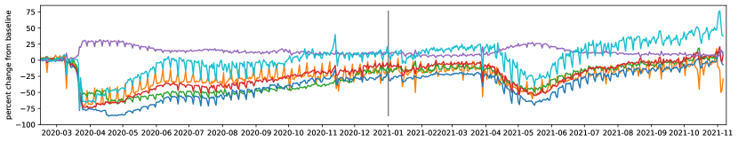
(a) India

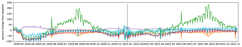
(b) Italy

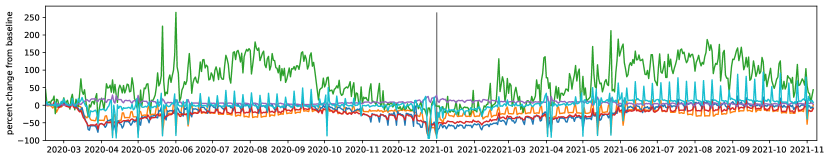
(c) Germany

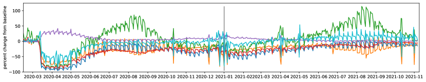
(d) Spain

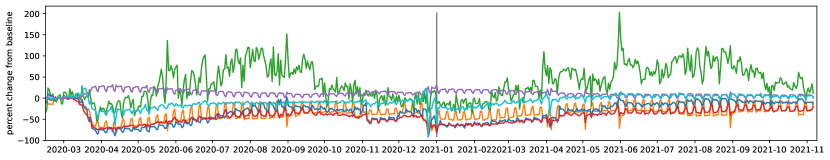
(e) United Kingdom

Figure 20. Mobility data for selected countries, gathered and published by Google [44]

Most vaccines need multiple applications to achieve a high level of protection. Often the time between the injections is regulated by recommendation relying on the product information and studies or different bureaucratic means that may depend on availability of vaccines and prioritising strategies.

For this simple model we choose a vaccine, which is administered twice like e.g. the vaccine of Biontech/Pfizer. We only use the type of susceptibles and an auxiliary type for the vaccines, see Table 7 (for a SIRD model including single vaccination, see Section 3.12). The interval between both injections is assumed to be fixed at least $\omega_{\nu}$ and is modeled as a reaction delay, denoted by a dashed arrow in the reaction scheme.

Table 7. Additional types needed to describe COVID-19 vaccination strategies.

Types	Interpretation
$V$	Vaccines
$S_{v,a}$	Susceptible individual with vaccination status $v\in\{0,1,2\}$ and approval $a\in\{0,1\}$

For reaction constants $\pi,\nu_{1},\nu_{2}>0$ and delays $\omega_{\pi},\omega_{\nu}>0$, the following rules describe type changes:

$$\emptyset \mathrel{\mathop{\dashrightarrow}_{\omega_{\pi}}} \;\pi V,$$ [Vaccine Production] (3.38)

$$V+ S_{0,1} \xrightarrow{\nu_{1}} \;S_{1,0} \mathrel{\mathop{\dashrightarrow}_{\omega_{\nu}}} \;S_{1,1},$$ [1st-Vaccination, delayed Authorisation for Vaccination]

$$V+ S_{1,1} \xrightarrow{\nu_{2}} \;S_{2,0},$$ [2nd-Vaccination]

The first rule describes the deterministic production of vaccines within time $\omega_{\pi}$, also indicated by a dashed arrow. Here we allow for the auxiliary type $V$ also the empty set on the source side of the rule. Whereas the second and third rules model vaccination based on availability $V$ of the vaccine. After the delay in the second rule of $\omega_{\nu}$ since getting the first dose, the single vaccinated susceptibles are marked / approved getting the second dose. By the rates $\nu_{1}$ and $\nu_{2}$ we model also different prioritisation of first and second vaccinations.

(a) $\nu_{1}=2$, $\nu_{2}=18$

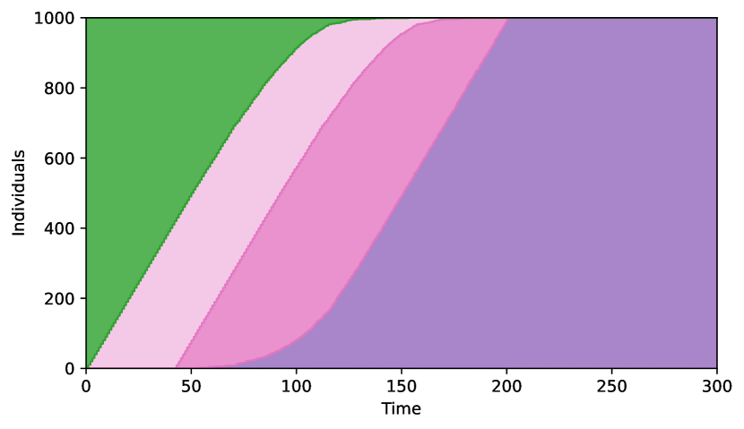
(b) $\nu_{1}=18$, $\nu_{2}=2$

(c) $\nu_{1}=10$, $\nu_{2}=10$

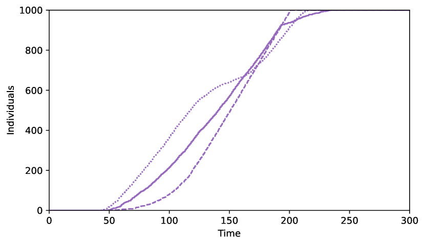
(d) twice vaccinated for different prioritisations

Figure 21. SSA simulations for simple vaccination model with different prioritisations $\nu$. $\pi=10$, $\omega_{\pi}=1$, $\omega_{\nu}=42$.

The SSA simulations in Figure 21 show the effects of different prioritisations with a given vaccine production and delays. For all first vaccination rates $\nu_{1}$ the curve for number of individuals with one vaccination is determined by the production $\frac{\pi}{\omega_{\pi}}$ until the waiting time $\omega_{\nu}=42$ for approval for the second injection is over for the first time. Then the available vaccines are distributed according to the prioritisations. When prioritising second vaccination in Figure 21(a) or treating them equally in Figure 21(c), the reservoir of approved individuals for the second injection is reduced more or less quickly. After that approved individuals get immediately vaccinated with the second injection. Thus the curves for $S_{1,0}$ and $S_{2,0}$ appear shifted in parallel in time, when $S_{1,1}$ almost vanishes. This may lead to sharp kinks in the curve for the number of twice vaccinated individuals, see Figure 21(c). Whereas when prioritising first vaccinations, like in Figure 21(b), the second vaccinations start slowly although a sufficient number of approved individuals is available. In Figure 21(d) the trajectories for the number of twice vaccinated individuals for the three prioritisations are compared. We observe that prioritisation of second vaccinations reaches faster a possible goal of, e.g. a fraction of $60\%$ twice vaccinated individuals.

3.12. Opinion Formation

One major difference between chemical particles and human individuals is opinions and the resulting behaviour. Vaccination is an important countermeasure for infectious deceases, but people have different opinions regarding the risk and benefit of them. Opinions are formed in groups and they may change based on incidences like severe consequences after vaccination. We reformulate basic models of opinion formation used for elections like [55] in the context of our framework. For simplicity we consider only two opinions, pro and contra vaccination, but for each opinion one group who can freely change opinions and one group of zealots who do not change their opinion. Echo camber or filter bubbles could be also included by using an effective incidence for opinion contacts instead of simple mass incidence, which is equivalent to the models introduced in [55]. For the vaccination process we distinguish between vaccinated and not vaccinated individuals, and adding a special sub-types $D_{p,2}$, $p\in\{0,1,2,3\}$, for individuals deceased – as an extreme – due to vaccination, see Table 8. For this more complex model we combine the SIRD model with vaccination and opinion formation in the rules of (3.12).

Table 8. The types of the standard SIR model with vaccination and opinion formation.

Type	Interpretation
$p\in\{0,1,2,3\}$	Sub-type for opinion:	$0$: pro vaccination (zealots),
		$1$: pro vaccination,
		$2$: contra vaccination
		$3$: contra vaccination (zealots)
$v\in\{0,1\}$	Sub-type for vaccination:	$0$: not vaccinated,
		$1$: vaccinated,
$S_{p,v}$	Susceptible individuals	with opinion $p$ and vaccination status $v$
$I_{p,v}$	Infectious individuals	with opinion $p$ and vaccination status $v$
$R_{p,v}$	Recovered individuals	with opinion $p$ and vaccination status $v$
$D_{p,v}$	Deceased individuals	with opinion $p$ and vaccination status $v$
$D_{p,2}$	Deceased individuals	with opinion $p$ and died due to vaccination

$$S_{2,v}+S_{p^{\prime},v^{\prime}} \xrightarrow{\mu_{1}} S_{1,v}+S_{p^{\prime},v^{\prime}}, \quad p^{\prime} \in\{0,1\},\ v,v^{\prime}\in\{0,1\},$$ [Convincing an Opponent]

$$S_{1,v}+S_{p^{\prime},v^{\prime}} \xrightarrow{\mu_{2}} S_{2,v}+S_{p^{\prime},v^{\prime}}, \quad p^{\prime} \in\{2,3\},\ v,v^{\prime}\in\{0,1\},$$ [Convincing an Supporter]

$$S_{p,0} \xrightarrow{\nu} S_{p,1}, \quad p \in\{0,1\},$$ [Vaccination of Willing]

$$S_{p,0} \xrightarrow{\eta} D_{p,2}, \quad p \in\{0,1\},$$ [Death by Vaccination]

$$S_{p,0}+I_{p^{\prime},0} \xrightarrow{\iota_{0}} I_{p,0}+I_{p^{\prime},0}, \quad p,p^{\prime} \in\{0,1,2,3\},$$ [Infection of unvaccinated]

$$S_{p,1}+I_{p^{\prime},0} \xrightarrow{\iota_{1}} I_{p,1}+I_{p^{\prime},0}, \quad p,p^{\prime} \in\{0,1,2,3\},$$ [Infection of vaccinated] (3.39)

$$I_{p,0} \xrightarrow{\rho_{0}} R_{p,0}, \quad p \in\{0,1,2,3\},$$ [Recovery of unvaccinated Infected]

$$I_{p,1} \xrightarrow{\rho_{1}} R_{p,1}, \quad p \in\{0,1,2,3\},$$ [Recovery of vaccinated Infected]

$$I_{p,0} \xrightarrow{\delta_{0}} D_{p,0}, \quad p \in\{0,1,2,3\},$$ [Death of unvaccinated Infected]

$$I_{p,1} \xrightarrow{\delta_{0}} D_{p,1}, \quad p \in\{0,1,2,3\},$$ [Death of vaccinated Infected]

$$S_{2,v}+D_{p,0} \xrightarrow{\gamma_{1}} S_{1,v}+D_{p,0}, \quad p \in\{0,1,2,3\},\ v,v^{\prime}\in\{0,1\},$$ [News about Death of unvaccinated

convince Vaccine Opponent]

$$S_{1,v}+D_{p,2} \xrightarrow{\gamma_{2}} S_{2,v}+D_{p,2}, \quad p \in\{0,1,2,3\},\ v,v^{\prime}\in\{0,1\},$$ [News about Death by Vaccination

scare off Vaccine Supporter]

We consider opinion formation only inside the group of susceptibles. The first two rules in (3.12) describe the change of opinions based on encountering an individual of the other group like an infection process. This is equivalent to the zealot model [10]. Note that opinions may change also after vaccination. The next rule models vaccination exclusively for people who are willing. The fourth rule generates deceased people due to vaccination. For the following six rules describing the infection process, recovery and death, we also include rules for infection of but not by vaccinated individuals. We do not include, e.g, spread of news directly, but describe the change of opinion based on extreme consequences of the behaviour like dying due to the virus because not vaccinated or due to the vaccination. We model this by the last two rules as encounters with deceased individuals $D_{p,2}$ and $D_{p,0}$ acting as ghosts and zealots for opponents and supporters, respectively.

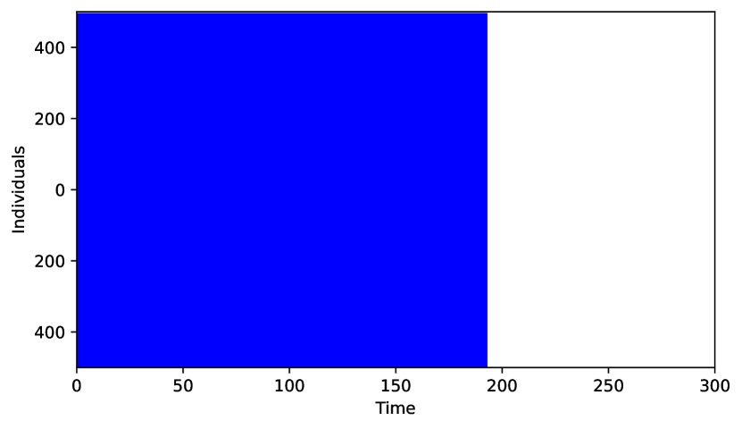
Opinion Dynamics

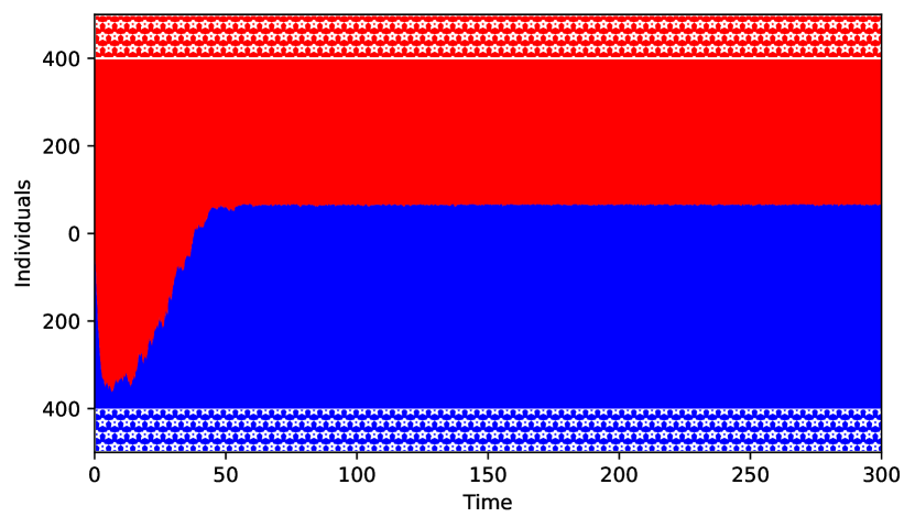
Opinion Dynamics

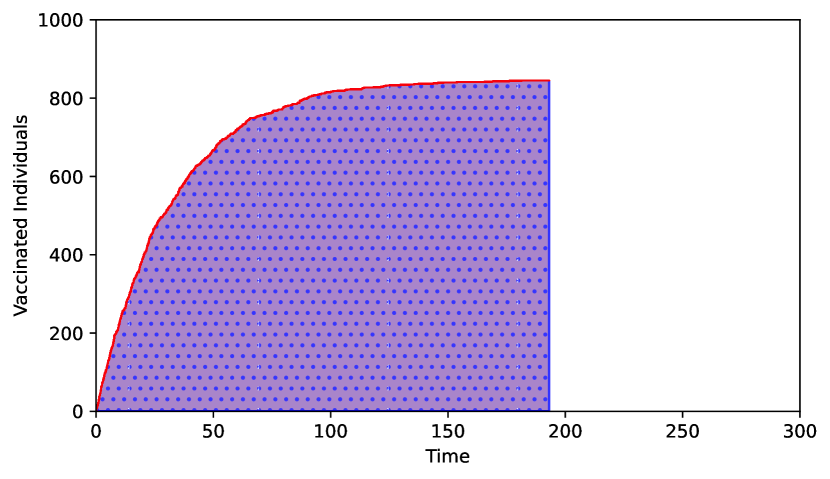
Vaccination

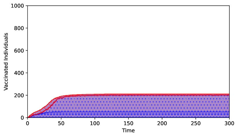
Vaccination

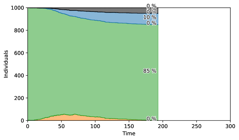
SIRD vs time

(a) Only Vaccination. ${\iota=\iota^{0}(1,0)}$, ${\rho=\rho^{0}(1,1)}$, ${\delta=\delta^{0}(1,1)}$, ${\eta=0}$.

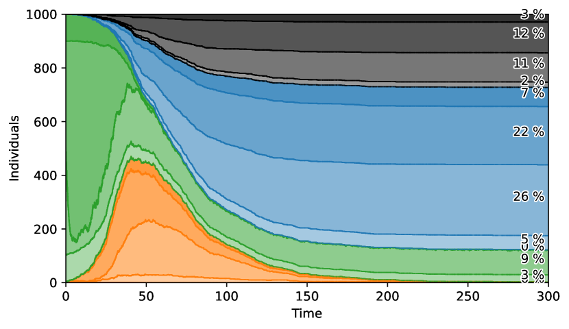
SIRD vs time

(b) Vaccination and Opinion Formation. ${\iota=\iota^{0}(1,0.1)}$, ${\rho=\rho^{0}(1,1.5)}$, ${\delta=\delta^{0}(1,0.5)}$, ${\eta=0.01}$.

Figure 22. SSA simulations for SIRD with vaccination and opinion formation. $\nu=0.025$, $\mu=(0.5,1.5)$, $\gamma=(10.,10.)$.

The SSA simulations for this, compared to the other models, more complex model are shown in Figure 22. To display the multidimensional data, we extracted the numbers with focus on different aspects, like opinion dynamics, vaccination and the accustomed stacked plot for epidemic numbers, and summarise over other quantities. Figure 22(a) show only the effect of vaccination. For this we use one opinion, supporting vaccination, and no death by vaccination, $\eta=0$. Here we assume complete immunity due to vaccination by setting $\iota=\iota^{0}(1,0)$. Thus the graph for vaccination shows only the number of vaccinated susceptible individuals. Due to the high vaccination rate $\nu=0.025$ the number of infectable individuals decreases very fast and the epidemic ends before reaching high peaks. At the end all remaining susceptible individuals are vaccinated. On the other hand in Figure 22(b), where we simulate the full model with supporters and opponents, each with unconvincable zealots, death by vaccination, and opinion formation, the results are different. At the beginning, both opinions are equally widespread with $20\%$ zealots each, but with a high rate of $\mu_{2}=1.5$ supporters are convinced to become opponents. Even after vaccination people change their opinion, leading to a small red dotted area of opponent but vaccinated individuals. However shortly thereafter, the mechanics of the infection works and the unvaccinated susceptible individuals are absorbed by the recovered or deceased states. Simultaneously opinions form by deterrent decease due to infection or, more rarely, vaccination. But since the vaccinations cannot be carried out quickly enough due to unwillingness, the epidemic breaks out. At the end apart from recovered individuals a small share of vaccinated susceptibles survive the epidemic without ever getting infected.

3.13. Mutations

The coronavirus has undergone multiple mutations since triggering a world wide pandemic. The general evolutionary principle is simple: the more prevalence of any coronavirus variant in the human population, the more likely are successful mutations as well. Virus are simple, their mutation rates are high. It is not necessarily the case that mutations lead to higher infectivity, some mutations might be neutral. However, there is evolutionary pressure to increase infectivity, as this clearly increases the fitness of the virus in Darwinian reasoning. The data also show that this is likely the case [39].

In order to incorporate evolutionary coronavirus dynamics, we introduce new types in Table 9. For a given set of mutants, we can describe the COVID-19 pandemic as a competitive system between mutants, see (3.40).

Table 9. Additional types needed to describe COVID-19 mutations.

Types	Interpretation
$m\in M$	coronavirus	mutant $m$
$I_{m},m\in M$	Infected with coronavirus	mutant $m$
$D_{m},m\in M$	Dead due coronavirus	mutant $m$

$$S+I_{m} \xrightarrow{\iota_{m}} I_{m}+I_{m}, \quad m\in M$$    [Infection] (3.40)

$$I_{m} \xrightarrow{\rho_{m}} R_{m}, \quad m\in M$$    [Recovery]

$$R_{m} \xrightarrow{\lambda_{m}} S, \quad m\in M$$    [Immunity Loss]

$$I_{m} \xrightarrow{\delta_{m}} D_{m}, \quad m\in M$$    [Death]

In this simple model (3.40), the different coronavirus mutants compete for susceptible people, and all transition events depend on the mutant involved. Especially the infectivity rate $\iota_{m}$ will differ as discussed in [39]. Recovery and immunity loss rules describe different responses of the immune system to different mutants in a very simplistic way. Also death rates $\delta_{m}$ will differ, as will hospitalisation numbers in general. We do not include cross-infection for different mutants, but cross-immunity.

Propensities with numbers:

$$\begin{split}\kappa_{1,m}({S},{I},{R},{D})&=\frac{\iota_{m}}{N}{S}{I}_{m},\\ \kappa_{2,m}({S},{I},{R},{D})&=\rho_{m}{I}_{m},\\ \kappa_{3,m}({S},{I},{R},{D})&=\lambda_{m}{R}_{m},\\ \kappa_{4,m}({S},{I},{R},{D})&=\delta_{m}{I}_{m},\\ \end{split}$$ (3.41)

where $m\in M$.

ODEs with fractions:

$$\begin{split}\frac{\mathop{}\!\mathrm{d}{\mathrm{S}}}{\mathop{}\!\mathrm{d}t}&=-\sum_{m\in M}\iota_{m}{\mathrm{S}}{\mathrm{I}}_{m}+\sum_{m\in M}\lambda_{m}{\mathrm{R}},\\ \frac{\mathop{}\!\mathrm{d}{\mathrm{I}}_{m}}{\mathop{}\!\mathrm{d}t}&=\iota_{m}{\mathrm{S}}{\mathrm{I}}_{m}-(\rho_{m}+\delta_{m}){\mathrm{I}}_{m},\\ \frac{\mathop{}\!\mathrm{d}{\mathrm{R}}_{m}}{\mathop{}\!\mathrm{d}t}&=\rho_{m}{\mathrm{I}}_{m}-\lambda_{m}{\mathrm{R}}_{m},\\ \frac{\mathop{}\!\mathrm{d}{\mathrm{D}}_{m}}{\mathop{}\!\mathrm{d}t}&=\delta_{m}{\mathrm{I}}_{m},\end{split}$$ (3.42)

where $m\in M$.

Individuals in mutation classes over time

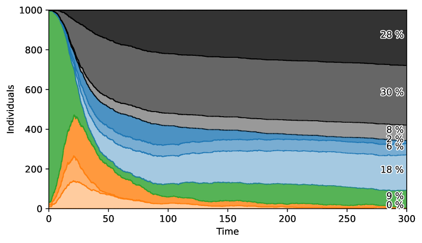
(a) seed $=0$.

Proportions of active Mutations over time

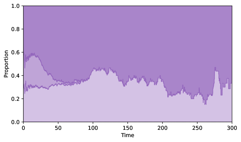
(b) seed $=0$.

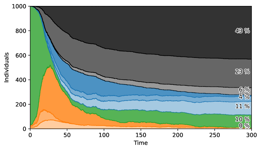
(c) seed $=1$.

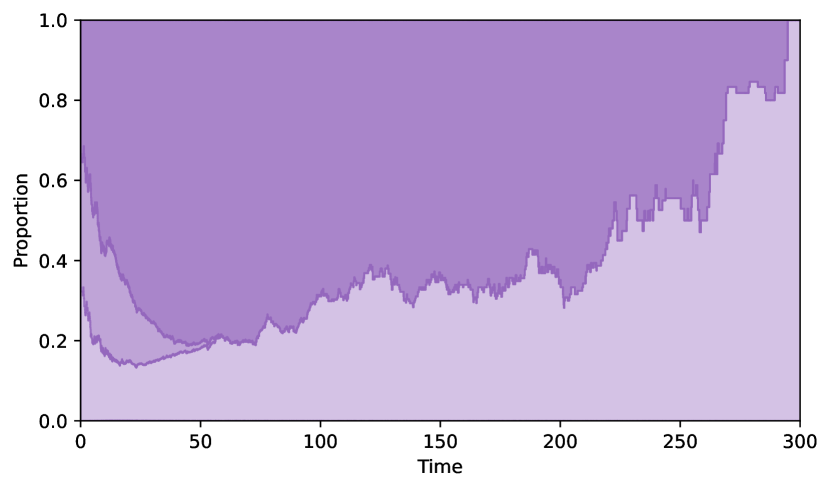
(d) seed $=1$.

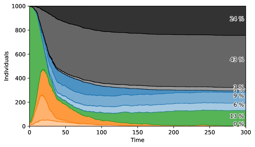
(e) seed $=8$.

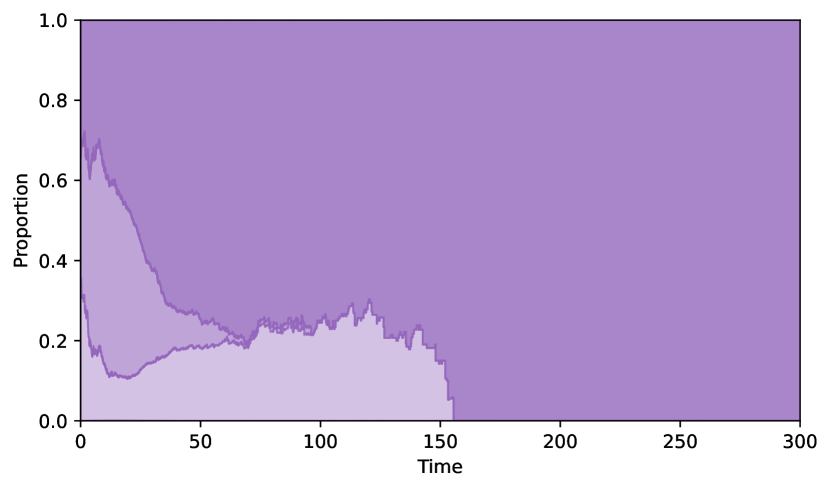
(f) seed $=8$.

Figure 23. SSA realisations for mutation model, Mutant 1: basis variant, Mutant 2: higher infection and death rate, Mutant 3: moderately higher infection and death rate and slight loss of immunity. $\iota=\iota^{0}(1.,2.,1.5)$, $\rho=\rho^{0}(1.0,1.0,1.0)$, $\delta=\delta^{0}(1.,10.,2.)$, $\lambda=(0.,0.,0.02)$.

For the SSA simulations in Figure 23 we consider three mutant variants. The index $m=1$ denotes the basis variant, $m=2$ a variant with higher infection rate and much higher death rate, $m=3$ one with moderately higher infection and death rate but slight loss of immunity. Starting with $10$ infectious individuals for each mutant, all three variants are competing for active infections. The proportion of infected per variant over time is displayed in the second column of Figure 23. Note that total number of infected for all variants changes significantly, for absolute numbers see first column. The variant $m=2$ with highest infection and death rate is erased very early. This is in accordance with often observed disappearance of very deadly mutants, due to infected rather die than infect new susceptible individuals. For the other two variants the outcome depends heavily on stochasticity, especially for the low absolute numbers at later times. Sometimes variant $m=3$, with higher mortality but additional loss of immunity, is predominant, like in Figures 23(b) and 23(f), sometimes variant $m=1$ overtakes variant $m=3$, see Figure 23(d).

4. Discussion And Outlook

We have proposed an epidemiological modeling framework for the COVID-19 dynamics, which introduces a systematic and mathematical consistent way to model all aspects of the COVID-19 pandemic, dependent on the questions being asked, policies investigated, and - not covered in this paper, but see Section 1.5 and future work - the available data. The framework would have been empty if we would not have introduced model outlines, in some cases complete models, furthermore code and simulations, for all aspects of the COVID-19 pandemic. We therefore believe we have established a new milestone on which future IT-based expert systems can help humanity to manage global pandemics more efficiently.

4.1. The Prognosis Problem of Mathematical Models

We would like to stress that if mathematical modelling exists in order to help managing a pandemic effectively, the predictive power of models, or family of models, as is the approach in this article, needs to be tested and finally established. Mathematical modelling might also just exist to focus minds of experts, and establish a discussion. Although we support this idea, a restriction on this limited focus would not bring mathematical modelling towards its true capability. With the advance of modern methods of applied mathematics and computational power we should and also can aim for much more. Unfortunately we could not identify true proven predictive power in any of the current mathematical models used during the pandemic. Some of the models might actually have prognostic power, but they rely more on the reputation of work groups or institutions rather than objective criteria. We call this current lack of predictive or prognostic power the fundamental prognosis problem, which is intrinsically related to Bayesian model selection, see Section 1.5. The reasons for the fundamental prognosis problem are manifold:

Complexity:

During the time course of an epidemic the background conditions change such that they are not covered by the current types, i.e. variables of a model. One has to realise that mathematical models are compact descriptions of reality, and therefore neglect circumstances which at a moment, or better a certain time frame, do not significantly contribute to the measured data. However, in a complex system such as an epidemic, the underlying mechanisms might change, therefore the number of variables needed to describe the system might increase.

Model Selection:

It is clear that single models, whatever their complexity, are parametrised with a certain data set from the past. Therefore the fundamental assumption is again that the conditions giving parameters their numerical value, or parameter range, should not have significantly changed when a prognosis is attempted.

Model Comparison:

In epidemiology, unlike for example in climate modelling, models are not regularly compared with each other to establish strength and weaknesses of prognostic power in certain situations. This would need the international and interdisciplinary cooperation of epidemiological modellers. There are also no established criteria with which prognostic power is measured. Such a discussion is long overdue.

Deterministic versus Stochastic Modeling:

A large misunderstanding by some experts and the general public is the lack of understanding of the intrinsic stochastic nature of an epidemic. Deterministic models are good enough in some circumstances, and therefore reliable, but only if the law of large numbers can be applied to all aspects of the model situation. In this case one can establish a sensitivity analysis, showing which parts of the model react most significantly if data are not reliable, or the underlying conditions change only slightly. However, in stochastic modeling the idea of a definitive time course has to be abandoned. It is replaced by the idea of an ensemble of time courses, which all can happen with certain probabilities. Prediction in a stochastic world therefore is more difficult, and has a very different meaning.

4.2. The Data

We have not covered in this article any methods and applications of statistics and data analysis in general, in particular we have not parametrised our models with real world data. This very important task, a highly complex topic in itself, is left to future considerations and publications. Here we give just some general observation relevant for the presented modelling framework. Most importantly, the COVID-19 pandemic has brought scientific data reading literally to the forefront of billons of people, a highly relevant development for science in general. Reading and listening to the latest infection numbers has become a part of daily routine by billions of people. Of course, like for mathematical modelling discussed in the previous Section 4.1, there are problems with standardisation of data as well, see [26]. The internet and modern IT-infrastructure have made data collection on a massive scale nevertheless feasible. One of the main institutions showing how this can be done is the Johns Hopkins University with its Coronavirus Ressource Center, [65]. But nearly all national or international organisations related to epidemiology, also newspapers and other institutions, have collected relevant data, see the references in [15], or the WHO [69]. The speed of data collection and display has generally improved [21]. Therefore, there should be plenty of scope to connect in a next step mathematical models and epidemiological data in a more continuous fashion as well.

It is important to not that a reliable epidemic model or expert system will have to incorporate a multitude of different data. For example, in order to learn from the effectiveness of policy measures, one needs a clear understanding of the nature of policies, for example lockdowns, and their duration. A good example of available data bases is the Oxford policy database [47].

4.3. Future Expert Systems

The two previous Sections 4.1 and 4.2 on mathematical models and data lead naturally to the question how these two streams of research can work together more effectively in future? A natural environment where these different mathematical and empirical research can converge can be expressed as an idea of a novel type of expert system, based on modern mathematical and computational methods, IT-developments and empirical science. We believe the following topics are the most important ones in a long list of choices and properties of such a novel expert system:

Rule-Based Systems:

Rule-based systems as exclusively used in this article have a huge advantage: they are easy to interpret once some basic intuition for rules can be acquired. This experience can also be acquired by non-mathematicians. Moreover, rules can be easily stored in computers. This should enable a way to use machine learning and artificial intelligence in several ways to aid successful prognosis of a pandemic time course, described below. As long as rule-based systems are simple enough, they can be extremely simply communicated to non-scientists. It has become more more evident, especially during the pandemic, that science in general needs to communicate better to be understood by the public.

Machine Learning, AI:

Future expert systems will rely on both mathematical modelling and machine learning. We use here the term machine learning in a general sense, the term includes also artificial intelligence. Artificial intelligence methods have made rapid progress in the last years, especially deep learning methods represent a leap forward in unsupervised automatic learning from data [62]. A typical application to the COVID-19 pandemic is given by [63]. That mathematical models and AI methods should be developed side by side is no contradiction. For example, the claim that deep learning alone could substitute mathematical modelling is far-fetched and dangerous. Mathematical modelling is hypothesis building of underlying mechanisms governing a process, in our case a pandemic process. In order to be able to do this, there needs to be some time invariance of these acting mechanisms. But as long as the time invariance is guaranteed, mechanisms are ideally identified by the mathematical model, and therefore policies can be put in place to manipulate them in a desired direction. Note that this is not the case if one relies on artificial intelligence approaches only. Artificial intelligence cannot identify mechanisms, it is simply not designed for this purpose.

However, machine learning and AI are needed in other ways, mostly for data integration into mathematical models, we discuss this as a next topic below. Another, perhaps less obvious help by machine learning techniques are Bayesian model selection algorithms. In fact this is so important, and so little discussed even within applied mathematics, that we gave a brief introduction in Section 1.6. Without a model framework where mathematical models are systematically able to be altered according to empirical evidence, mathematical models will not help to understand epidemics, the prognosis problem, see Section 4.1, will not be overcome. There are other uses for machine learning as well. For example, one can contemplate how non-mathematical experts formulate their insight into the pandemic by verbal descriptions. By machine learning this verbal description, in addition with mathematical consistency checks, is translated into a rule-based system. It could be a very fruitful way how a future expert system interacts with different experts from different fields, expressing their opinions and subsequently validating and investigating such believe systems with the help of empirical data.

Data Incorporation:

Machine learning and AI are urgently needed to integrate real world data into future expert systems based on mathematical models. As we have discussed in Section 4.2, more and more data are becoming available online, or at least in a machine readable form. All mathematical models need to be parametrised, and the more data are available for that purpose, the better. There are some promising new approaches for model parameter estimation that should be very suitable for epidemiological modelling problems, like SINDy [16], [36]. An application to epidemiology is reference [32]. In emergency situations like a pandemic, the parametrisation of mathematical models needs best be done in a nearly continuous way, in order to make future expert systems successful. As discussed in Section 4.2, the data retrieval aspect needed for such a strategy becomes better and better due to the development of better IT infrastructures in different countries. There is another aspect related to Bayesian model selection, Section 1.6, and the prognosis problem, Section 4.1. According to the criteria given, all selected models will only be the best Bayesian choice for some limited time, until the empirical data suggest new underlying mechanisms are at work which have not previously be incorporated. There is a shift from one best model to another in model space, see Section 1.5.3. This can be interpreted as a kind of early warning system, if properly implemented: there are new trends detected in the data suggesting underlying mechanisms are not all time invariant any more, some new process partially governs the pandemic situation.

4.4. Expert Systems And Experts

It has become apparent during the coronavirus pandemic that the role of experts, so mostly the general scientific, and more specifically the medical sciences community, had an opinion game to play with the general public, and the politicians representing them, see [41]. Different interests collided, and necessary health care interventions were not always taken up unchallenged. For example, the COVID-19 pandemic with its clearly global scale, had to balance health care concerns with economic activity, the latter severely restricted in lockdowns and under other pandemic driven policies. This opinion formation game involving science and the public was clearly in addition dynamic, with all the main players, scientists, politicians and public, having a relative increase or decrease of influence on decision making processes or public majority opinion and support over time. At the beginning of the pandemic in Europe in March 2020, mostly individual scientists soon became popular experts in the news, but also in panels set up by different governments. The advise given to the public, kept simple, such as ’flattening the curve’, was relatively well communicated, perhaps due to its simplicity. However, even in this case, there is much more behind the scientific concept that would have needed to be communicated [9]. This shows that there is a limit of complexity reduction which should be expected of the public. At that time hospitals were clearly overwhelmed and rapid action was needed. This shows that also the speed of decision making needed is time variable.

In general the public supported measures such as social distancing and lockdowns. But of course, after now two years of living with coronavirus, public support and a wish to return to normality increased. Indeed, the price to pay were heavy, both in economic and psychological terms. For example, school children and students suffered from a lack of personal face to face support, which is often needed. The science community was not prepared well for the pandemic, for example there was a clear lack of incorporation of psychologists, sociologists, and political scientists.

To discuss the role of experts, expert panels, governmental institutions and the public during the COVID-19 pandemic so far, it is worthwhile to compare the scientific response to the COVID-19 pandemic and climate change in general. Two UN institutions come to mind, the World Health Organisation (WHO), [70] , and the International Panel of Climate Change (IPCC), [33]. In some aspects the WHO and the IPCC are very similar in their respective areas of expertise, the WHO officially monitors health risks on a global scale, as does the IPCC monitor risks for the global stability of the climate. However, in other respects the organisations are completely different. The WHO is an old institution, founded in $1948$, and more or less resembles national health institutions, with which it is closely cooperating and relying on their data. The IPCC is a scientific panel in contrast, assembled for a single purpose, to assess scientifically risks related to the global climate. Other than the WHO the IPPC has a well functioning peer review process, and tries to incorporate divergent scientific evidence in single reports, which it releases from time to time, [7], [58]. The policies recommended are based on risk assessment [64], but even the assessment criteria are under constant discussion. Comparing the scientific reputation and scientific independence, we believe the IPCC has much more to offer than the WHO, as internal procedures and internal decision making follow rigorous procedures that are open to review by the public. In conclusion, we believe that the COVID-19 pandemic has shown that the example of the IPCC should trigger a rethinking how experts working on epidemiological problems and policies should come together on an international level to discuss health risks. As pandemics and climate act on different time scales, the reporting velocity obviously needs to be accelerated. This approach would also be a relief for many experts working in epidemiology on a national level, perhaps even working in national governmental institutions. The impact of the COVID-19 pandemic was immense, and to give scientific evidence has immense potential impact and responsibility. It is a much better situation for science when scientists working on a local level can refer to an international scientific opinion, that has gone through a rigorous peer review process.

We like to end this discussion on the role expert systems, as the one proposed in this article, can play in future. It is telling that during the COVID-19 pandemic so far there was no comparison of the predictive power of different national or university driven epidemiological models. This did neither happen on the national level, nor on the international level. Decision making was nearly exclusively driven by statistics, not by any mathematical models. There are only very few counterexamples to be found. But mostly these models were taken as hand-waving tools by different scientists when interacting with the public. In addition, thousands of preprints were published in different archives suggesting new mathematical models in rapid sequence. Without a global peer review process, just like the IPCC does for publications in the climate change area, all this effort is very likely good for nothing, or not for much. After a mathematical model has been established, there comes the simulation phase, which at the same time must be interpreted as the predictive phase, see Section 4.1. In the climate change area there are many different climate models running in different countries. Their outcomes are discussed and compared rigorously, perhaps eventually taken up in reports by the IPCC. A future expert systems, or different expert systems dedicated to epidemiological situations should try to go the same way. Predictive power and even criteria for predictive power have to be established. This should include a discussion how predictive power can be increased by systematic incorporation of more details into the models, like is known to be the case with mesh refinements in weather predictions.

The whole effort would not be worth it if the scientific evidence does not point to the predictive power of mathematical models in epidemiology. However, we believe that the range of models as discussed in this and future articles does establish a feasible way to go. If future expert systems based on mathematical models can be embedded into an international interdisciplinary team of scientists, just like it was the case in the climate change area, we could find a way to manage future epidemics more profoundly. Given the destruction of global habitat, the next global epidemic is very likely to happen fast again [30].

Appendix A Parameters

Here we list the sets of parameters used throughout the simulation scenarios in this article. If a parameter does not appear in the list, it is equal to the parameter of the base model. We like to emphasize that parameters are chosen according to rules of thumb, they should resemble reasonable values. However, none of these parameters has been derived from real world data. This parameter estimation problem we leave to future publications. We also provide here the names of the jupyter notebooks used to create the according figures.

Table 10. Parameters for simulations

model		jupyter notebook
Parameter	Value	Meaning	Fig.
SIRD (base model)		RBSEa1_SIRD.ipynb
$N$	$1000$	total population	5
$I_{0}^{0}$	$3$	initial infectious
$T$	$300$	maximum time
$\iota^{0}$	$0.2$	infection rate
$\rho^{0}$	$0.02$	recovery rate
$\delta^{0}$	$0.01$	death rate
seed	$0$	random seed
SIRDa (age)		RBSEa1_SIRDa.ipynb
$a\in A$	{1, 2, 3}	index for age classes	6
$I_{0}$	$(1,1,1)$	initial infectious
$p$	$(0.25,0.5,0.25)$	initial population shares
$C$	$\left(\begin{smallmatrix}76&38&5\\ 38&67&13\\ 5&13&9\end{smallmatrix}\right)$	contact matrix
$\rho$	$\rho^{0}(1.5,1.0,0.5)$	recovery rates
$c=q\cdot s\cdot i$	$0.0047567053338882$	product of calibration, infectivity and susceptibility factors
$\delta$	$\delta^{0}(0.25,1.0,2.0)$	death rates
$\iota$	$c\cdot C$	infection rates (${R_{0}\approx 6.67}$)	6(a)
$\iota$	$c\cdot\left(\begin{smallmatrix}1.0&1.0&0.2\\ 1.0&1.0&0.2\\ 0.2&0.2&1.0\end{smallmatrix}\right)\circ C$	infection rates with reduced contact to elderly class (${R_{0}\approx 6.59}$) ($\circ$: Hadamard product)	6(b)
SIRDc (testing)		RBSEa1_SIRDc.ipynb
$c\in$	$\{0,1,2\}$	index for test classes	7
$I_{0}$	$(3,0,0)$	initial infectious
$\vartheta$	$0.04$	rate of testing
$\vartheta_{S}$	$\vartheta$	rate of testing of susceptibles
$\vartheta_{I}$	$\vartheta$	rate of testing of infected
$\vartheta_{R}$	$\vartheta$	rate of testing of recovered
$\lambda$	$0.02$	loss of information	7(a), 7(b), 7(c), 7(d)
$\lambda$	$0.2$	loss of information	7(e), 7(f)
$\iota$	$\iota^{0}\left(\begin{smallmatrix}1.&1.&1.\\ 1.&1.&1.\end{smallmatrix}\right)$	infection rates	7(a), 7(b)
$\rho$	$\rho^{0}(1.,1.,1.)$	recovery rates
$\delta$	$\delta^{0}(1.,1.,1.)$	death rates
$\iota$	$\iota^{0}\left(\begin{smallmatrix}0.7&0.2&0.9\\ 0.9&0.2&1.\end{smallmatrix}\right)$	infection rates	7(c), 7(d), 7(e), 7(f)
$\rho$	$\rho^{0}(1.,1.5,1.)$	recovery rates
$\delta$	$\delta^{0}(1.0,0.5,1.0)$	death rates
SIRDresp (functional response)		RBSEa1_SIRDresp.ipynb
$T$	$500$	maximum time	8
$\iota({I};\mu)$	$\frac{\iota^{0}}{1+\mu\frac{{I}}{N}}$	infection rate with functional response
$\mu$	$1$	functional response parameter	8(a)
$\mu$	$10$	functional response parameter	8(b)
SIRDcresp (testing, functional response)		RBSEa1_SIRDcresp.ipynb
$T$	$500$	maximum time	9
$c\in$	$\{0,1,2\}$	index for test classes
$I_{0}$	$(3,0,0)$	initial infectious
$\vartheta$	$0.04$	rate of testing
$\vartheta_{S}$	$\vartheta$	rate of testing of susceptibles
$\vartheta_{I}$	$\vartheta$	rate of testing of infected
$\vartheta_{R}$	$\vartheta$	rate of testing of recovered
$\lambda$	$0.1$	loss of information
$\iota$	$\iota({I};\mu)\left(\begin{smallmatrix}0.7&0.2&0.9\\ 0.9&0.2&1.\end{smallmatrix}\right)$	infection rates
$\iota({I};\mu)$	$\frac{\iota^{0}}{1+\mu\frac{{I}_{1}}{N}}$	infection rate with functional response dependent on tested infectious
$\rho$	$\rho^{0}(1.,1.5,1.)$	recovery rates
$\delta$	$\delta^{0}(1.0,0.5,1.0)$	death rates
$\mu$	$1$	functional response parameter	9(a)
$\mu$	$10$	functional response parameter	9(b)
SIRDh (hospitalisation)		RBSEa1_SIRDh.ipynb
$T$	$500$	maximum time	11
$h\in$	$\{0,1\}$	index for hospitalisation classes
$I_{0}$	$(3,0)$	initial infectious
$\iota$	$\iota^{0}(1.0,0.5)$	infection rates
$\rho$	$\rho^{0}(1.0,1.2)$	recovery rates
$\delta$	$\delta^{0}(1.0,0.1)$	death rates
$\eta({I}_{1})$	$\eta_{0}\frac{H_{\max}-{I}_{1}}{N}$	hospitalisation rates
$H_{\max}$	$0$	hospitalisation capacity	11(a)
$H_{\max}$	$500$	hospitalisation capacity	11(b)
$H_{\max}$	$25$	hospitalisation capacity	11(c)
$H_{\max}$	$100$	hospitalisation capacity	11(d), 11(e), 11(f)
$\iota(\vartheta,\lambda)$	$\iota\cdot f(\vartheta,\lambda)$	infection rates with response	11(e), 11(f)
$\vartheta$	$\frac{{I}_{0}+{I}_{1}}{N}$	response based on total infectious	11(e)
$\lambda$	$10$	response parameter
$\vartheta$	$\frac{{I}_{1}}{H_{\max}}$	response based on hospitalised infectious	11(f)
$\lambda$	$1$	response parameter
SIRDlock (lockdown)		RBSEa1_SIRDlock.ipynb
$\rho$	$\rho^{0}$	recovery rate	4
$\delta$	$\delta^{0}$	death rate
$\iota(t)$	$\begin{cases}\iota_{0}\cdot(1-\lambda_{s})&\text{for }T_{s}\leq t<T_{e},\\ \iota_{0}&\text{else}\end{cases}$	time dependent infection rate
$T_{s}$	$25$	lockdown start time	12(a)
$T_{e}$	$50$	lockdown end time
$\lambda_{s}$	$0.9$	lockdown severeness / contact reduction
$T_{s}$	$25$	lockdown start time	12(b)
$T_{e}$	$100$	lockdown end time
$\lambda_{s}$	$0.6$	lockdown severeness / contact reduction
Im (immunity)		RBSEa1_Im.ipynb
$m\in$	$\{0,1,2,\ldots,7\}$	index for immunity classes	14
$N$	$1000$	total population
$I_{0}$	$(0,0,0,0,0,0,0,0)$	initial infected
$\iota$	$100$	infection rate
$\{(d_{m},i_{m})\}$	$\{(5,0.0)$, $(4,0.2)$, $(3,0.6)$, $(2,0.8)$, $(6,1.0)$, $(8,0.7)$, $(10,0.3)$, $(12,0.1)\}$	immunity profile
$\phi_{m}$	$\frac{1}{d_{m}}$	immunity change rate, final loss rate
SIRDm (infectivity)		RBSEa1_SIRDm.ipynb
$m\in$	$\{0,\ldots,M\}$	index for infectivity classes	15, 16, 17(b)
$\iota_{m}$	$\iota^{0}c_{I}i_{m}$	infection rates
$\phi_{m}$	$\frac{1}{d_{m}}$	infectivity change rates, final recovery rate
$\delta_{m}$	$\delta^{0}c_{I}i_{m}$	death rates
$c_{I}$	$\frac{\sum_{m\in\{0,\ldots,M\}}d_{m}\cdot i_{m}}{\sum_{m\in\{0,\ldots,M\}}d_{m}}=2.5$	proportionality factor for infection / death rates
$M$	$0$	maximum index for infectivity classes	15(a), 15(b)
$I_{0}$	$3$	initial infectious
$\{(d_{m},i_{m})\}$	$\{(50,0.4)\}$	infectivity profile
$M$	$1$	maximum index for infectivity classes	15(c), 15(d)
$I_{0}$	$(3,0)$	initial infectious
$\{(d_{m},i_{m})\}$	$\{(10,0.0),(40,0.5)\}$	infectivity profile
$M$	$3$	maximum index for infectivity classes	15(e), 15(f)
$I_{0}$	$(3,0,0)$	initial infectious
$\{(d_{m},i_{m})\}$	$\{(10,0.0),(15,1.0),(25,0.2)\}$	infectivity profile
$M$	$7$	maximum index for infectivity classes	16(a),16(b)
$I_{0}$	$(3,0,0,0,0,0,0,0)$	initial infectious
$\{(d_{m},i_{m})\}$	$\{(5,0.0)$, $(4,0.2)$, $(3,0.6)$, $(2,0.8)$, $(6,1.0)$, $(8,0.7)$, $(10,0.3)$, $(12,0.1)\}$	infectivity profile
$M$	$7$	maximum index for infectivity classes	16(c),16(d)
$I_{0}$	$(3,0,0,0,0,0,0,0)$	initial infectious
$\{(d_{m},i_{m})\}$	$\{(5,0.4)$, $(4,0.4)$, $(3,0.4)$, $(2,0.4)$, $(6,0.4)$, $(8,0.4)$, $(10,0.4)$, $(12,0.4)\}$	constant infectivity profile
$M$	$99$	maximum index for infectivity classes	16(e),16(f)
$I_{0}$	$(3,0,\ldots,0)$	initial infectious
$\{(d_{m},i_{m})\}$	$\{(\frac{50}{M+1},0.4),\ldots,(\frac{50}{M+1},0.4)$ = $\{(0.5,0.4),\ldots,(0.5,0.4)\}$	constant infectivity profile
$(M+1)\in$	$\{1,2,\ldots,10,20,\ldots,100\}$	maximum number for infectivity classes	17(b)
$I_{0}$	$(3,0,\ldots,0)$	initial infectious
$\{(d_{m},i_{m})\}$	$\{(\frac{50}{M+1},0.4),\ldots,(\frac{50}{M+1},0.4)$ = $\{(0.5,0.4),\ldots,(0.5,0.4)\}$	constant infectivity profile
SIRDmdup (infectivity, discrete updates)		RBSEa1_SIRDmdup.ipynb
$m$	$0$	index for infectivity classes	6
$I_{0}$	$1$	initial infectious
$\iota_{0}$	$\iota^{0}$	infection rate
$\omega_{0}$	$\frac{1}{\rho^{0}}=50$	discrete delay for recovery
$\delta_{0}$	$\delta^{0}$	death rate
SIRDb (behaviour) for face-masks		RBSEa1_SIRDb.ipynb
$b\in$	$\{1,2\}$	index for behaviour classes	18
$\iota$	$\iota^{0}\left(\begin{smallmatrix}0.5&0.7\\ 0.7&1.0\end{smallmatrix}\right)$	infection rates
$\delta$	$\delta^{0}(1.,1.)$	death rates
$\rho$	$\rho^{0}\left(\begin{smallmatrix}1.0&0.0\\ 0.0&1.0\end{smallmatrix}\right)$	recovery rates	18(a), 18(b)
$(\sigma_{1,2}^{S},\sigma_{2,1}^{S})$	$(0.0,0.0)$	switching rate for susceptibles
$(\sigma_{1,2}^{I},\sigma_{2,1}^{I})$	$(0.0,0.0)$	switching rate for infectious
$(\sigma_{1,2}^{R},\sigma_{2,1}^{R})$	$(0.0,0.0)$	switching rate for recovered
$I_{0}$	$(0,3)$	initial susceptibles	18(a)
$S_{0}$	$N(0.0,1.0)-I_{0}=(0,997)$	initial susceptibles
$I_{0}$	$(3,0)$	initial susceptibles	18(b)
$S_{0}$	$N(1.0,0.0)-I_{0}=(997,0)$	initial susceptibles
$\rho$	$\rho^{0}\left(\begin{smallmatrix}1.0&0.0\\ 0.9&0.1\end{smallmatrix}\right)$	recovery rates	18(c), 18(d)
$I_{0}$	$(0,3)$	initial susceptibles
$S_{0}$	$N(0.2,0.8)-I_{0}=(200,797)$	initial susceptibles
$(\sigma_{1,2}^{S},\sigma_{2,1}^{S})$	$(0.01,0.02)$	switching rate for susceptibles	18(c)
$(\sigma_{1,2}^{I},\sigma_{2,1}^{I})$	$(0.01,0.02)$	switching rate for infectious
$(\sigma_{1,2}^{R},\sigma_{2,1}^{R})$	$(0.005,0.02)$	switching rate for recovered
$(\sigma_{1,2}^{S}({I})$, $\sigma_{2,1}^{S}({I}))$	$(0.01,0.02\cdot(1+10\cdot\frac{{I}_{1}+{I}_{2}}{N}))$	switching rate for susceptibles depending on total infected	18(d)
$(\sigma_{1,2}^{I}({I})$, $\sigma_{2,1}^{I}({I}))$	$(0.01,0.02\cdot(1+10\cdot\frac{{I}_{1}+{I}_{2}}{N}))$	switching rate for infectious depending on total infected
$(\sigma_{1,2}^{R}({I})$, $\sigma_{2,1}^{R}({I}))$	$(0.005,0.02\cdot(1+10\cdot\frac{{I}_{1}+{I}_{2}}{N}))$	switching rate for recovered depending on total infected
SIRDb (behaviour) for lockdowns		RBSEa1_SIRDb.ipynb
$b\in$	$\{1,2\}$	index for behaviour classes	19
$I_{0}$	$(0,3)$	initial susceptibles
$S_{0}$	$N(0.0,1.0)-I_{0}=(0,997)$	initial susceptibles
$\iota$	$\iota^{0}\left(\begin{smallmatrix}1-\lambda_{s}&\sqrt{1-\lambda_{s}}\\ \sqrt{1-\lambda_{s}}&1.0\end{smallmatrix}\right)$	infection rates
$\rho$	$\rho^{0}\left(\begin{smallmatrix}1&0\\ 0&1\end{smallmatrix}\right)$	recovery rates
$\delta$	$\delta^{0}(1.,1.)$	death rates
$T_{s}$	$25$	lockdown start time	19(a), 19(c), 19(e)
$T_{e}$	$50$	lockdown end time
$\lambda_{s}$	$0.9$	lockdown severity
$T_{s}$	$25$	lockdown start time	19(b), 19(d), 19(f)
$T_{e}$	$100$	lockdown end time
$\lambda_{s}$	$0.6$	lockdown severity
$(\sigma_{1,2}^{S},\sigma_{2,1}^{S})$ = $(\sigma_{1,2}^{I},\sigma_{2,1}^{I})$ = $(\sigma_{1,2}^{R},\sigma_{2,1}^{R})$	$\begin{cases}(0.0,0.0),&t\in[0,T_{s}),\\ (0.0,1.0),&t\in[T_{s},T_{e}),\\ (1.0,0.0),&t\in[T_{e},T]\end{cases}$	time dependent switching rates	19(a), 19(b)
$(\sigma_{1,2}^{S},\sigma_{2,1}^{S})$ = $(\sigma_{1,2}^{I},\sigma_{2,1}^{I})$ = $(\sigma_{1,2}^{R},\sigma_{2,1}^{R})$	$\begin{cases}(0.0,0.0),&t\in[0,T_{s}),\\ (0.0,0.1),&t\in[T_{s},T_{e}),\\ (1.0,0.0),&t\in[T_{e},T]\end{cases}$	time dependent switching rates	19(c),19(d)
$(\sigma_{1,2}^{S},\sigma_{2,1}^{S})$ = $(\sigma_{1,2}^{I},\sigma_{2,1}^{I})$ = $(\sigma_{1,2}^{R},\sigma_{2,1}^{R})$	$\begin{cases}(0.0,0.0),&t\in[0,T_{s}),\\ (0.1,0.9),&t\in[T_{s},T_{e}),\\ (0.5,0.5),&t\in[T_{e},T]\end{cases}$	time dependent switching rates	19(e), 19(f)
VSv,a (vaccination)		RBSEa1_VSva.ipynb
$v\in$	$\{0,1,2\}$	index for vaccination class	21
$a\in$	$\{0,1\}$	index for vaccination approval class
${S}_{0}$	$\left(\begin{smallmatrix}0&N\\ 0&0\\ 0&0\end{smallmatrix}\right)$	initial susceptibles for vaccination
$\omega_{\pi}$	$1$	discrete delay for vaccine production
$\pi$	$10$	vaccine net production after $\omega_{\pi}$
$\omega_{\nu}$	$42$	discrete delay for second vaccination
$\nu_{1}$	$2$	rate for first vaccination of approved	21(a)
$\nu_{2}$	$18$	rate for second vaccination of approved
$\nu_{1}$	$18$	rate for first vaccination of approved	21(b)
$\nu_{2}$	$2$	rate for second vaccination of approved
$\nu_{1}$	$10$	rate for first vaccination of approved	21(c)
$\nu_{2}$	$10$	rate for second vaccination of approved
SIRDp,v (opinion formation, vaccination)		RBSEa1_SIRDpv.ipynb
$p\in$	$\{0,1,2,3\}$	index for opinion class	22
$v\in$	$\{0,1\}$	index for vaccination class
$\nu$	$0.025$	vaccination rate
$\mu$	$(0.5,1.5)$	rates of convincing an opponent / supporter
$\gamma$	$(10.0,10.0)$	rates of news convincing an opponent / scare off a supporter
$I_{0}$	$\left(\begin{smallmatrix}0&0\\ 3&0\\ 0&0\\ 0&0\\ \end{smallmatrix}\right)$	initial infectious	22(a)
$S_{0}$	$\left(\begin{smallmatrix}0&0\\ 997&0\\ 0&0\\ 0&0\\ \end{smallmatrix}\right)$	initial susceptibles
$\iota$	$\iota^{0}(1.0,0.0)$	infection rates
$\rho$	$\rho^{0}(1.0,1.0)$	recovery rates
$\delta$	$\delta^{0}(1.0,1.0)$	death rates
$\eta$	$0.0$	rate of death by vaccination
$I_{0}$	$\left(\begin{smallmatrix}0&0\\ 1&0\\ 2&0\\ 0&0\\ \end{smallmatrix}\right)$	initial infectious	22(b)
$S_{0}$	$\left(\begin{smallmatrix}100&0\\ 399&0\\ 398&0\\ 100&0\\ \end{smallmatrix}\right)$	initial susceptibles
$\iota$	$\iota^{0}(1.0,0.1)$	infection rates
$\rho$	$\rho^{0}(1.0,1.5)$	recovery rates
$\delta$	$\delta^{0}(1.0,0.5)$	death rates
$\eta$	$0.01$	rate of death by vaccination
SIRDm (mutations)		RBSEa1_SIRDm.ipynb
$m\in$	$\{1,2,3\}$	index for mutation class	23
${I}_{0}$	$(10,10,10)$	initial infectious
${S}_{0}$	$970$	initial susceptibles
$\iota$	$\iota^{0}(1.0,2.0,1.5)$	infection rates
$\rho$	$\rho^{0}(1.0,1.0,1.0)$	recovery rates
$\delta$	$\delta^{0}(1.0,10.0,2.0)$	death rates
$\lambda$	$(0.0,0.0,0.02)$	loss of immunity rates
seed	$0$	random seed	23(a), 23(b)
seed	$1$	random seed	23(c), 23(d)
seed	$8$	random seed	23(e), 23(f)

References

- [1] D. Alonso, S. Bauer, M. Kirkilionis, L. Kreusser, and L. Sbano, Generalised gillespie algorithm for simulations in a rule-based epidemiological model framework, in preparation, (2021).
- [2] M. an der Heiden and O. Hamouda, Schätzung der aktuellen Entwicklung der SARS-CoV-2- Epidemie in Deutschland – Nowcasting, Epidemiologisches Bulletin, 2020 (2020), pp. 10–15.
- [3] T. Aquino and M. Dentz, Chemical continuous time random walks, Phys. Rev. Lett., 119 (2017), p. 230601.
- [4] J. Arino and C. C. McCluskey, Effect of a sharp change of the incidence function on the dynamics of a simple disease, Journal of Biological Dynamics, 4 (2010), pp. 490–505. Publisher: Taylor & Francis _eprint: https://doi.org/10.1080/17513751003793017.
- [5] C. Aschwanden, Five reasons why COVID herd immunity is probably impossible, Nature, 591 (2021), pp. 520–522.
- [6] C. E. Bcheraoui, H. Weishaar, F. Pozo-Martin, and J. Hanefeld, Assessing COVID-19 through the lens of health systems’ preparedness: time for a change, Global Health, 16 (2020), pp. 964–980.
- [7] S. Beck and M. Mahony, The ipcc and the new map of science and politics, Wiley Interdisciplinary Reviews: Climate Change, 9 (2018).
- [8] M. Boguñá, L. F. Lafuerza, R. Toral, and M. A. Serrano, Simulating non-markovian stochastic processes, Phys. Rev. E, 90 (2014), p. 042108.
- [9] M. Boumans, Flattening the curve is flattening the complexity of covid-19., Hist Philos Life Sci, 43 (2021), p. 18.
- [10] D. Braha and M. A. M. de Aguiar, Voting contagion: Modeling and analysis of a century of u.s. presidential elections, PLOS ONE, 12 (2017), pp. 1–30.
- [11] F. Brauer and C. Castillo-Chavez, Mathematical models in population biology and epidemiology, vol. 2, Springer, 2012.
- [12] D. Breda, O. Diekmann, W. de Graaf, A. Pugliese, and R. Vermiglio, On the formulation of epidemic models (an appraisal of kermack and mckendrick)., J Biol Dyn, 6 Suppl 2 (2012), pp. 103–117.
- [13] C. E. Brook and A. P. Dobson, Bats as ‘special’ reservoirs for emerging zoonotic pathogens, Trends in Microbiology, 23 (2015), pp. 172–180.
- [14] K. P. Burnham, D. R. Anderson, and K. P. Burnham, Model selection and multimodel inference : a practical information-theoretic approach, Springer, New York, 2002.
- [15] S. Callaghan, Covid-19 is a data science issue, Patterns, 1 (2020).
- [16] K. Champion, S. Brunton, and J. Kutz, Discovery of nonlinear multiscale systems: Sampling strategies and embeddings, SIAM Journal on Applied Dynamical Systems, 18 (2019), pp. 312–333.
- [17] A. Cori, N. M. Ferguson, C. Fraser, and S. Cauchemez, A New Framework and Software to Estimate Time-Varying Reproduction Numbers During Epidemics, American Journal of Epidemiology, 178 (2013), pp. 1505–1512.
- [18] A. Danchin and G. Turinici, Immunity after COVID-19: Protection or sensitization?, Mathematical Biosciences, 331 (2021), p. 108499.
- [19] O. Diekmann, J. A. P. Heesterbeek, and M. G. Roberts, The construction of next-generation matrices for compartmental epidemic models, J. R. Soc. Interface, 7 (2010), pp. 873–885.
- [20] M. Domijan and M. Kirkilionis, Graph theory and qualitative analysis of reaction networks, NETWORKS AND HETEROGENEOUS MEDIA, 3 (2008).
- [21] E. Dong, H. Du, and L. Gardner, An interactive web-based dashboard to track covid-19 in real time., Lancet Infect Dis, 20 (2020), pp. 533–534.
- [22] S. N. Ethier and T. G. Kurtz, Markov processes: characterization and convergence, vol. 282, John Wiley & Sons, 2009.
- [23] N. Ford, H. K. Holmer, R. Chou, P. Villeneuve, A. Baller, M. Van Kerkhove, and B. Allegranzi, Mask use in community settings in the context of covid-19: A systematic review of ecological data, EClinical Medicine, 38 (2021).
- [24] C. Gaebler, Z. Wang, J. C. Lorenzi, F. Muecksch, S. Finkin, M. Tokuyama, A. Cho, M. Jankovic, D. Schaefer-Babajew, T. Y. Oliveira, M. Cipolla, C. Viant, C. O. Barnes, Y. Bram, G. Breton, T. Hägglöf, P. Mendoza, A. Hurley, M. Turroja, K. Gordon, K. G. Millard, V. Ramos, F. Schmidt, Y. Weisblum, D. Jha, M. Tankelevich, G. Martinez-Delgado, J. Yee, R. Patel, J. Dizon, C. Unson-O’Brien, I. Shimeliovich, D. F. Robbiani, Z. Zhao, A. Gazumyan, R. E. Schwartz, T. Hatziioannou, P. J. Bjorkman, S. Mehandru, P. D. Bieniasz, M. Caskey, and M. C. Nussenzweig, Evolution of antibody immunity to SARS-CoV-2, Nature, 591 (2021), pp. 639–644.
- [25] C. Gardiner, Stochastic Methods: A Handbook for the Natural and Social Sciences, Springer Series in Synergetics, Springer Berlin Heidelberg, 2009.
- [26] L. Gardner, J. Ratcliff, E. Dong, and A. Katz, A need for open public data standards and sharing in light of covid-19, The Lancet Infectious Diseases, 21 (2021), p. e80.
- [27] D. Gillespie, Master equations for random walks with arbitrary pausing time distributions, Physics Letters A, 64 (1977), pp. 22 – 24.
- [28] D. T. Gillespie, A general method for numerically simulating the stochastic time evolution of coupled chemical reactions, Journal of Computational Physics, 22 (1976), pp. 403 – 434.
- [29] V. Haldane, C. D. Foo, S. M. Abdalla, A.-S. Jung, M. Tan, S. Wu, A. Chua, M. Verma, P. Shrestha, S. Singh, T. Perez, S. M. Tan, M. Bartos, S. Mabuchi, M. Bonk, C. McNab, G. K. Werner, R. Panjabi, A. Nordström, and H. Legido-Quigley, Health systems resilience in managing the COVID-19 pandemic: lessons from 28 countries, Nat Med, 27 (2021), pp. 964–980.
- [30] J. Hassell, T. Newbold, A. Dobson, Y. Linton, L. Franklinos, D. Zimmerman, and K. Pagenkopp Lohan, Towards an ecosystem model of infectious disease., Nat Ecol Evol, 5 (2021), pp. 907–918.
- [31] S. Heroy, I. Loaiza, A. Pentland, and N. O’Clery, COVID-19 policy analysis: labour structure dictates lockdown mobility behaviour, Journal of the Royal Society, Interface, 18 (2021), p. 20201035.
- [32] J. Horrocks and C. Bauch, Algorithmic discovery of dynamic models from infectious disease data., Sci Rep, 10 (2020), p. 7061.
- [33] IPCC, https://en.wikipedia.org/wiki/intergovernmental_panel_on_climate_change, Wikipedia, (2021).
- [34] P. Jentsch, M. Anand, and C. T. Bauch, Prioritising COVID-19 vaccination in changing social and epidemiological landscapes: a mathematical modelling study, The Lancet Infectious Diseases, 21 (2021), pp. 1097–1106.
- [35] J. Jost, Mathematical Concepts, Springer, 2015.
- [36] K. Kaheman, S. Brunton, and J. Kutz, Automatic differentiation to simultaneously identify nonlinear dynamics and extract noise probability distributions from data, arXiv preprint arXiv:2009.08810, (2020).
- [37] W. O. Kermack and A. G. McKendrick, A contribution to the mathematical theory of epidemics, Proceedings of the Royal Society of London. Series A., 115 (1927), pp. 700–721.
- [38] P. Klepac, A. J. Kucharski, A. J. Conlan, S. Kissler, M. L. Tang, H. Fry, and J. R. Gog, Contacts in context: large-scale setting-specific social mixing matrices from the bbc pandemic project, medRxiv, (2020).
- [39] B. Korber, W. Fischer, S. Gnanakaran, C. LaBranche, E. O. Saphire, and D. C. Montefiori, Tracking changes in sars-cov-2 spike: Evidence that d614g increases infectivity of the covid- 19 virus, Cell, 182 (2020), pp. 812–827.
- [40] J. Ladyman and K. Wiesner, What Is a Complex System?, Yale University Press, 2020.
- [41] A. Lavazza and M. Farina, The role of experts in the covid-19 pandemic and the limits of their epistemic authority in democracy., Front Public Health, 8 (2020), p. 356.
- [42] E. Lavezzo, E. Franchin, C. Ciavarella, G. Cuomo-Dannenburg, L. Barzon, C. Del Vecchio, L. Rossi, R. Manganelli, A. Loregian, N. Navarin, D. Abate, M. Sciro, S. Merigliano, E. De Canale, M. C. Vanuzzo, V. Besutti, F. Saluzzo, F. Onelia, M. Pacenti, S. G. Parisi, G. Carretta, D. Donato, L. Flor, S. Cocchio, G. Masi, A. Sperduti, L. Cattarino, R. Salvador, M. Nicoletti, F. Caldart, G. Castelli, E. Nieddu, B. Labella, L. Fava, M. Drigo, K. A. Gaythorpe, K. E. Ainslie, M. Baguelin, S. Bhatt, A. Boonyasiri, O. Boyd, L. Cattarino, C. Ciavarella, H. L. Coupland, Z. Cucunubá, G. Cuomo-Dannenburg, B. A. Djafaara, C. A. Donnelly, I. Dorigatti, S. L. van Elsland, R. FitzJohn, S. Flaxman, K. A. Gaythorpe, W. D. Green, T. Hallett, A. Hamlet, D. Haw, N. Imai, B. Jeffrey, E. Knock, D. J. Laydon, T. Mellan, S. Mishra, G. Nedjati-Gilani, P. Nouvellet, L. C. Okell, K. V. Parag, S. Riley, H. A. Thompson, H. J. T. Unwin, R. Verity, M. A. Vollmer, P. G. Walker, C. E. Walters, H. Wang, Y. Wang, O. J. Watson, C. Whittaker, L. K. Whittles, X. Xi, N. M. Ferguson, A. R. Brazzale, S. Toppo, M. Trevisan, V. Baldo, C. A. Donnelly, N. M. Ferguson, I. Dorigatti, and A. Crisanti, Suppression of a SARS-CoV-2 outbreak in the Italian municipality of Vo’, Nature, 584 (2020), pp. 425–429.
- [43] D. Lewis, Superspreading drives the COVID pandemic - and could help to tame it, Nature, 590 (2021), pp. 544–546.
- [44] G. LLC, Google covid-19 community mobility reports, 2021. [Online; accessed 13-July-2021].
- [45] N. MacDonald, Biological Delay Systems, Chapter 10, Cambridge University Press, 1989.
- [46] D. J. C. MacKay, Information Theory, Inference and Learning Algorithms, Cambridge University Press, 2003.
- [47] A. Mahdi, P. Błaszczyk, P. Dłotko, D. Salvi, and T. Chan…, Oxcovid19 database, a multimodal data repository for better understanding the global impact of covid-19, Scientific Reports, (2021).
- [48] S. Mallapaty, Is the coronavirus getting deadlier? The data are inconclusive, Nature, 590 (2021).
- [49] , Israel is first to see COVID-infection drop from vaccines, Nature, 590 (2021), p. 85.
- [50] N. Masuda and L. E. C. Rocha, A gillespie algorithm for non-markovian stochastic processes, SIAM REVIEW, 60 (2018), pp. 95–115.
- [51] H. McCallum, N. Barlow, and J. Hone, How should pathogen transmission be modelled?, Trends in Ecology & Evolution, 16 (2001), pp. 295–300.
- [52] T. R. Mercer and M. Salit, Testing at scale during the COVID-19 pandemic, Nat Rev Genet, 22 (2021), pp. 415–426.
- [53] J. C. Miller, A Note on the Derivation of Epidemic Final Sizes, Bulletin of Mathematical Biology, 74 (2012), pp. 2125–2141.
- [54] J. Mossong, N. Hens, M. Jit, P. Beutels, K. Auranen, R. Mikolajczyk, M. Massari, S. Salmaso, G. S. Tomba, J. Wallinga, J. Heijne, M. Sadkowska-Todys, M. Rosinska, and W. J. Edmunds, Social contacts and mixing patterns relevant to the spread of infectious diseases, PLOS Medicine, 5 (2008), pp. 1–1.
- [55] J. Müller, V. Hösel, and A. Tellier, Filter bubbles, echo chambers, and reinforcement: Tracing populism in election data. arXiv:2007.03910.
- [56] P. Nouvellet, S. Bhatia, A. Cori, K. E. Ainslie, M. Baguelin, S. Bhatt, A. Boonyasiri, N. F. Brazeau, L. Cattarino, L. V. Cooper, H. Coupland, Z. M. Cucunuba, G. Cuomo-Dannenburg, A. Dighe, B. A. Djaafara, I. Dorigatti, O. D. Eales, S. L. van Elsland, F. F. Nascimento, R. G. FitzJohn, K. A. Gaythorpe, L. Geidelberg, W. D. Green, A. Hamlet, K. Hauck, W. Hinsley, N. Imai, B. Jeffrey, E. Knock, D. J. Laydon, J. A. Lees, T. Mangal, T. A. Mellan, G. Nedjati-Gilani, K. V. Parag, M. Pons-Salort, M. Ragonnet-Cronin, S. Riley, H. J. T. Unwin, R. Verity, M. A. Vollmer, E. Volz, P. G. Walker, C. E. Walters, H. Wang, O. J. Watson, C. Whittaker, L. K. Whittles, X. Xi, N. M. Ferguson, and C. A. Donnelly, Reduction in mobility and COVID-19 transmission, Nature Communications, 12 (2021), pp. 1–9.
- [57] M. O’Driscoll, G. Ribeiro Dos Santos, L. Wang, D. A. Cummings, A. S. Azman, J. Paireau, A. Fontanet, S. Cauchemez, and H. Salje, Age-specific mortality and immunity patterns of SARS-CoV-2, Nature, 590 (2021), pp. 140–145.
- [58] R. K. Pachauri, M. R. Allen, V. R. Barros, J. Broome, W. Cramer, R. Christ, J. A. Church, L. Clarke, Q. Dahe, and P. Dasgupta, Climate change 2014: synthesis report. contribution of working groups i, ii and iii to the fifth assessment report of the intergovernmental panel on climate change, IPCC, https://epic.awi.de/id/eprint/37530 (2014), p. 151.
- [59] S. Palmer, N. Cunniffe, and R. Donnelly, COVID-19 hospitalization rates rise exponentially with age, inversely proportional to thymic T-cell production, Journal of the Royal Society, Interface, 18 (2021), p. 20200982.
- [60] N. Powdthavee, Y. Riyanto, E. Wong, J. Yeo, and Q. Chan, When face masks signal social identity: Explaining the deep face-mask divide during the covid-19 pandemic., PLoS One, 16 (2021), p. e0253195.
- [61] K. Prem, K. v. Zandvoort, P. Klepac, R. M. Eggo, N. G. Davies, C. for the Mathematical Modelling of Infectious Diseases COVID-19 Working Group, A. R. Cook, and M. Jit, Projecting contact matrices in 177 geographical regions: An update and comparison with empirical data for the covid-19 era, PLOS Computational Biology, 17 (2021), pp. 1–19.
- [62] S. Russell and P. Norvig, Artificial Intelligence: A Modern Approach., Pearson Higher Education, 2021.
- [63] F. Shamout, Y. Shen, N. Wu, A. Kaku, and J. Park…, An artificial intelligence system for predicting the deterioration of covid-19 patients in the emergency department, NPJ Digital …, (2021).
- [64] P. Tangney, Understanding climate change as risk: a review of ipcc guidance for decision-making, Journal of Risk Research, 23 (2020), pp. 1424–1439.
- [65] J. H. University, Coronavirus ressource center, https://coronavirus.jhu.edu/map.html, (2021).
- [66] P. van den Driessche and J. Watmough, Reproduction numbers and sub-threshold endemic equilibria for compartmental models of disease transmission, Mathematical Biosciences, 180 (2002), pp. 29–48.
- [67] J. Wallinga, P. Teunis, and M. Kretzschmar, Using data on social contacts to estimate age-specific transmission parameters for respiratory-spread infectious agents, American journal of epidemiology, 164 (2006), pp. 936–944.
- [68] Z. Wang, F. Schmidt, Y. Weisblum, F. Muecksch, C. O. Barnes, S. Finkin, D. Schaefer-Babajew, M. Cipolla, C. Gaebler, J. A. Lieberman, T. Y. Oliveira, Z. Yang, M. E. Abernathy, K. E. Huey-Tubman, A. Hurley, M. Turroja, K. A. West, K. Gordon, K. G. Millard, V. Ramos, J. D. Silva, J. Xu, R. A. Colbert, R. Patel, J. Dizon, C. Unson-O’Brien, I. Shimeliovich, A. Gazumyan, M. Caskey, P. J. Bjorkman, R. Casellas, T. Hatziioannou, P. D. Bieniasz, and M. C. Nussenzweig, mRNA vaccine-elicited antibodies to SARS-CoV-2 and circulating variants, Nature, 592 (2021).
- [69] WHO, Coronavirus dashboard, https://covid19.who.int, (2021).
- [70] , https://en.wikipedia.org/wiki/world_health_organization, Wikipedia, (2021).
- [71] D. Wodarz, N. L. Komarova, and L. M. Schang, Role of high-dose exposure in transmission hot zones as a driver of SARS-CoV-2 dynamics, Journal of the Royal Society, Interface, 18 (2021), p. 20200916.
- [72] R. Wölfel, V. M. Corman, W. Guggemos, M. Seilmaier, S. Zange, M. A. Müller, D. Niemeyer, T. C. Jones, P. Vollmar, C. Rothe, M. Hoelscher, T. Bleicker, S. Brünink, J. Schneider, R. Ehmann, K. Zwirglmaier, C. Drosten, and C. Wendtner, Virological assessment of hospitalized patients with COVID-2019, Nature, 581 (2020), pp. 465–469.
- [73] H. Zeberg and S. Pääbo, The major genetic risk factor for severe covid-19 is inherited from neanderthals, Nature, (2020).
- [74] , A genomic region associated with protection against severe covid-19 is inherited from neandertals, Proceedings of the National Academy of Sciences, (2021).