Distinctive features of oscillatory phenomena in reconstructions of the topological structure of electron trajectories on complex Fermi surfaces

Abstract

We consider the behavior of classical and quantum oscillations in metals with complex Fermi surfaces near the directions of $\,{\bf B}\,$ corresponding to changes in the topological structure of the dynamical system describing the semiclassical motion of quasiparticles along the Fermi surface. The transitions through the boundaries of change in this structure are accompanied by sharp changes in the picture of oscillations, the form of which depends in the most essential way on the topological type of the corresponding reconstruction. We list here the main features of such changes for all topological types of elementary reconstructions and discuss the possibilities of experimental identification of such types based on these features.

I Introduction

In this work, we would like to consider features of oscillatory phenomena observed in reconstructions of the topological structure of the system describing the semiclassical motion of electrons on the Fermi surface in the presence of an external magnetic field. As is well known, this system has the form

$${\dot{\bf p}}\,\,\,\,=\,\,\,\,{e\over c}\,\,\left[{\bf v}_{\rm gr}({\bf p})\,\times\,{\bf B}\right]\,\,\,\,=\,\,\,\,{e\over c}\,\,\left[\nabla\epsilon({\bf p})\,\times\,{\bf B}\right]\,\,\,,$$ (I.1)

where $\,\epsilon({\bf p})\,$ is the electronic dispersion relation in the crystal for a given conduction band. The relation $\,\epsilon({\bf p})\,$ represents a smooth 3-periodic function in the $\,{\bf p}$ - space with periods equal to the reciprocal lattice vectors. As it is easy to see, the system (I.1) conserves the energy value $\,\epsilon({\bf p})\,$ and the projection of the quasimomentum on the direction of the magnetic field, and, as a consequence, its trajectories are given by the intersections of periodic surfaces $\,\epsilon({\bf p})\,=\,{\rm const}\,$ by planes, orthogonal to $\,{\bf B}\,$ (Fig. 1).

Figure 1: The geometry of the trajectories of system (I.1) in the space of quasimomenta.

From the physical point of view, points in $\,{\bf p}$ - space, which differ by reciprocal lattice vectors, represent the same physical state, so that the system (I.1) can be considered, in fact, as a system on the three-dimensional torus $\,\mathbb{T}^{3}\,$ obtained from $\,\mathbb{R}^{3}\,$ by factorization over reciprocal lattice vectors. The periodic surfaces $\,\epsilon({\bf p})\,=\,{\rm const}\,$ after such factorization become also compact two-dimensional surfaces embedded in $\,\mathbb{T}^{3}\,$ (as a rule, in a topologically nontrivial way). As is well known, in the theory of normal metals, among all energy levels, the Fermi energy plays the most important role, and thus the most important is the structure of the trajectories of system (I.1) on the Fermi surface $\,\epsilon({\bf p})\,=\,\epsilon_{F}\,$.

The great importance of the geometry of trajectories of system (I.1) for the theory of galvanomagnetic phenomena in metals was established in the works of the school of I.M. Lifshits in the 1950s (see lifazkag ; lifpes1 ; lifpes2 ; lifkag1 ; lifkag2 ; lifkag3 ; etm ; KaganovPeschansky ). At this time many important and interesting examples of nontrivial behavior of the trajectories of system (I.1) on complex Fermi surfaces, as well as the corresponding regimes of behavior of magnetic conductivity in strong magnetic fields, were considered. In the general case, the geometry of the trajectories of system (I.1) starts to play a decisive role under the condition $\,\omega_{B}\tau\gg 1\,$, which also implies sufficient purity of the sample under study, as well as its low temperature ($T\sim 1{\rm K}$) during the corresponding measurements.

Somewhat later, in the work of S.P. Novikov MultValAnMorseTheory the problem of general classification of trajectories of the system (I.1) for arbitrary relations $\,\epsilon({\bf p})\,$ was set, which was then fruitfully investigated in his topological school (see zorich1 ; dynn1992 ; dynn1 ; zorich2 ; DynnBuDA ; dynn2 ; dynn3 ). Topological results obtained at the school of S.P. Novikov, made it possible, in particular, to determine new topological characteristics observable in the conductivity of normal metals (PismaZhETF ; UFN ), and also led to the discovery of new, previously unknown, types of trajectories of the system (I.1) (Tsarev ; dynn2 ), leading to new regimes of behavior of magnetic conductivity (ZhETF1997 ; TrMian ). On the whole, to date, it can be stated that the study of the Novikov problem has led ultimately to a complete classification of all types of trajectories of the system (I.1), as well as to a description of the corresponding regimes of behavior of magnetic conductivity in strong magnetic fields (see, for example dynn3 ; UFN ; BullBrazMathSoc ; JournStatPhys ; UMNObzor ; ObzorJetp ).

It should be noted that a very important role in the study of the Novikov problem is played by the study of the set of closed trajectories of the system (I.1) on the Fermi surface. Moreover, it can even be argued that knowledge of the structure of the set of closed trajectories on a given Fermi surface actually determines the types of all other trajectories on it and, in particular, allows one to describe their global geometric properties. It can also be noted that the set of nonsingular closed trajectories is always an open set on the Fermi surface and is locally stable with respect to small changes in the parameters of the problem (in particular, small changes in the Fermi energy or the direction of the magnetic field). From the above fact it follows, actually, that usually the space of parameters defining the system (I.1) should be divided into regions in which the topological structure of system (I.1) can be considered unchanged, while at the boundaries of such regions abrupt changes in the structure of (I.1) occur. Besides that, any change in the structure of trajectories of (I.1) on the Fermi surface is always associated with a reconstruction of the structure of closed trajectories on it, which, in fact, also determines the structure of other trajectories.

In this work, we will be primarily interested in the dependency of the topological structure of system (I.1) on the direction of the magnetic field (Fig. 2). A typical picture of the boundaries separating different topological structures of (I.1) on the corresponding angular diagram (on the unit sphere $\,\mathbb{S}^{2}$) was discussed in the most general case in OsobCycle , where it was also indicated that the most convenient tool for observing it is the study of oscillatory phenomena (classical or quantum) for different directions of $\,{\bf B}$. The latter circumstance is due to the fact that changes in the topological structure of the system (I.1) always cause the disappearance (and the appearance of new ones) of extreme trajectories, which play a central role in describing oscillatory phenomena in strong magnetic fields (cyclotron resonance, the de Haas - Van Alphen effect, the Shubnikov - de Haas effect, etc.). Thus, the boundaries separating different topological structures of system (I.1) are, in fact, also the boundaries at which abrupt changes in the picture of classical or quantum oscillations occur under small changes of the direction of $\,{\bf B}$.

Figure 2: Regions on a part of the unit sphere corresponding to different topological structures of system (I.1) on the Fermi surface and the boundaries of reconstructions of this structure separating these regions (schematically).

As was shown in OsobCycle , the ‘‘net’’ of boundaries dividing the angular diagram into regions of a fixed topological structure of system (I.1) is generally quite complex and consists of ‘‘elementary’’ segments, each of which corresponds to some ‘‘elementary’’ reconstruction of the structure of system (I.1). The number of ‘‘elementary’’ segments can be generally infinite, in particular, the density of such segments becomes infinite near the directions of $\,{\bf B}\,$ corresponding to the appearance of open trajectories on the Fermi surface (Fig. 3). The paper OsobCycle also describes all the ‘‘elementary’’ reconstructions of the topological structure of (I.1) on the Fermi surface that arise in the generic situation. Each of these reconstructions corresponds, in particular, to the disappearance and appearance of extreme trajectories of a very special form, determined by its topological type. As we have already said, each of the segments of the reconstructions of the structure of (I.1) (one-dimensional curves in Fig. 2 and 3) corresponds to an elementary reconstruction of a certain topological type, while topological types of reconstructions corresponding to different segments, generally speaking, are different.

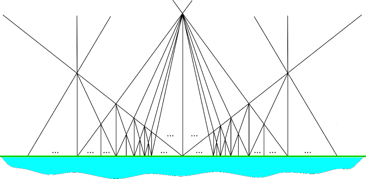
Figure 3: Dense net of boundaries of elementary reconstructions of the structure of (I.1), accumulating near a boundary of the appearance of open trajectories on the Fermi surface (schematically).

The main purpose of this work is to consider the features of observable oscillatory phenomena at the time of a change in the topological structure of the system (I.1) on the Fermi surface. As we will see, each of the ‘‘elementary’’ reconstructions of this structure has its own peculiarities in the behavior of oscillations, which, in particular, can be very useful in the experimental determination of the topological types of such reconstructions.

II Topological types of elementary reconstructions and the distinctive features of the picture of oscillatory phenomena for reconstructions of different types

As we have already said, reconstructions of the topological structure of the system (I.1) on the Fermi surface will mean for us topological reconstructions of the set of closed trajectories on this surface. In fact, as we have already noted above, the knowledge of the set of closed trajectories on the Fermi surface makes it possible to describe also trajectories of other types on it. The set of closed trajectories for generic directions of $\,{\bf B}\,$ is a finite set of (nonequivalent) cylinders bounded by singular closed trajectories on their bases (Fig. 4). The structure of the set of cylinders of closed trajectories (their position on the Fermi surface and the scheme of their gluing with carriers of other trajectories and with each other) is locally stable for small rotations of $\,{\bf B}\,$ and can change only for special directions of $\,{\bf B}\,$ when it becomes a non-generic structure. More precisely, to change the topological structure of (I.1), it is necessary to change the direction of $\,{\bf B}\,$ so that the height of one (or several) cylinder of closed trajectories becomes zero, i.e. we need the disappearance of a cylinder of closed trajectories, followed by the appearance of a new cylinder of low height (or several cylinders). The sets of directions of $\,{\bf B}\,$ corresponding to the moment of a reconstruction are one-dimensional curves on the angular diagram (on the unit sphere $\,\mathbb{S}^{2}$), whose union forms a ‘‘net’’ of directions of $\,{\bf B}\,$, corresponding to the reconstructions of the structure of (I.1) on the Fermi surface.

Figure 4: A ‘‘nontrivial’’ cylinder of closed trajectories bounded by singular trajectories on its bases.

As in the work OsobCycle , we will not pay attention here to the disappearance and appearance of ‘‘trivial’’ cylinders of closed trajectories, i.e. cylinders, at least one of the bases of which contracts to a single singular point (Fig. 5), and we will consider only reconstructions of cylinders, both bases of which are ‘‘nontrivial’’ (Fig. 4). In the generic case, we can assume that on each of the bases of such cylinders there is exactly one singular point of the system (I.1), and each of the bases represents one of the figures shown at Fig. 6. At the moment of reconstruction of the system (I.1), a ‘‘cylinder of zero height’’, containing two singular points of (I.1) connected by singular trajectories, appears on the Fermi surface. For each of the ‘‘elementary’’ reconstructions of the structure of (I.1), the corresponding ‘‘zero-height cylinder’’ represents a flat graph lying in a plane orthogonal to $\,{\bf B}\,$, and topologically is equivalent to one of the figures shown in Fig. 7. As was shown in OsobCycle , to determine the topological type of the ‘‘elementary’’ reconstruction of the system (I.1), it suffices to fix the topological type of the corresponding ‘‘cylinder of zero height’’ and indicate whether the group velocities at two singular points are co-directed, or directed opposite to each other.

Figure 5: A ‘‘trivial’’ cylinder of closed trajectories on the Fermi surface.

Figure 6: Possible types of bases of ‘‘nontrivial’’ cylinders of closed trajectories.

Figure 7: ‘‘Cylinders of zero height’’ arising at the moments of a reconstruction of the topological structure of system (I.1) on the Fermi surface.

The most important circumstance in the situation under consideration is that on each of the cylinders of small height, up to its disappearance, there exist extreme closed trajectories of the system (I.1) (having an extreme circulation period or area in comparison with close trajectories), disappearing together with the corresponding cylinder (Fig. 8). When a new cylinder of closed trajectories appears, new extreme trajectories appear on it, which differ from the disappeared ones in their geometry. As a consequence, each reconstruction of the topological structure of system (I.1) is followed by a sharp change in the picture of oscillatory phenomena in a strong magnetic field, which is a convenient tool for observing the above described ‘‘net’’ of directions of $\,{\bf B}\,$ at the angular diagram. It must be said that extreme closed trajectories arising on cylinders of small height have certain peculiarities in comparison with ordinary extreme trajectories, namely, they contain sections that are very close to singular points of the system (I.1). This circumstance leads, in particular, to an unlimited increase in the circulation period along such trajectories with a decrease in the height of the cylinder, as well as to a number of other features that arise, for example, when observing the phenomenon of cyclotron resonance (see, for example OsobCycle ).

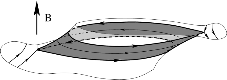
Figure 8: Extremal closed trajectory on a vanishing (appearing) cylinder of closed trajectories near the moment of a reconstruction of the topological structure of system (I.1) on the Fermi surface.

In this work, however, we would like to consider in more detail the features of extreme trajectories and the corresponding oscillatory phenomena that arise during each of the elementary reconstructions of the structure of (I.1), which, from our point of view, can be rather useful in the experimental study of a complete picture of reconstructions of the topology of this system on complex Fermi surfaces. As is well known (see, for example, etm ; Kittel ; Abrikosov ), for description of oscillatory phenomena, in fact, two types of closed extremal trajectories are important, namely, trajectories with an extreme orbital period and trajectories with an extreme area in comparison with trajectories close to them. Trajectories of the first type, as a rule, play a decisive role in the description of classical oscillatory phenomena (classical cyclotron resonance), while trajectories of the second type are important in describing quantum oscillatory phenomena (de Haas - van Alphen effect, Shubnikov - de Haas effect and etc.). Quite often, in reality, the same trajectory can be extreme from both the first and the second point of view, as a rule, this is the case for centrally symmetric sections of the Fermi surface. In most of the situations we consider below, however, this will not be the case, so we need to immediately divide the extreme trajectories into the two indicated types.

As we have already said, we will consider here cylinders of closed trajectories with ‘‘nontrivial’’ bases containing one singular point of the system (I.1). It is easy to see that the circulation period along closed trajectories on each of these cylinders increases infinitely (logarithmically) when approaching each of the bases. As a consequence, each of these cylinders must have at least one extremal trajectory with a minimum orbital period in comparison with trajectories close to it.

As for the area of closed trajectories, it is easy to see that it remains finite at the bases of the cylinders. Its derivative with respect to the distance to the corresponding base, however, goes to infinity (according to the logarithmic law) and can have a positive or negative sign, depending on the geometry of the cylinder. As for trajectories of the first type, this circumstance is also due to the presence of singular points on the bases of the cylinders and is associated with the local geometry of the trajectories near these points. Depending on the signs of the derivative of area with respect to the height on both bases, the cylinder of closed trajectories may or may not contain extreme trajectories of the second type. Fig. 9 shows examples of both cylinders containing extremal trajectories of the second type (a, b) and a cylinder that does not contain such a trajectory (c). It can be noted here that the extreme trajectory in Fig. 9a has a minimal area, while the extreme trajectory in Fig. 9b has the maximum area compared to trajectories close to them.

Figure 9: Cylinders of closed trajectories containing trajectories of extreme (minimum and maximum) area (a and b), and a cylinder not containing trajectories of extreme area (c).

Thus, it can be seen that any reconstruction of the structure of (I.1) is always accompanied by a sharp change in the picture of oscillations when observing, for example, the classical cyclotron resonance, while the picture of the de Haas - van Alphen or the Shubnikov - de Haas oscillations may contain no abrupt changes (if cylinders of small height on both sides of the reconstruction do not contain trajectories of extreme area). Special note should be made about the reconstructions of (I.1), which have central symmetry. In this case, the central sections of cylinders of small height always represent extreme trajectories of both the first and the second type.

In the most general case, cylinders of small height can contain extreme trajectories of both types, which, however, do not coincide with each other. In this case, although the reconstruction of (I.1) is accompanied by sharp changes in the pictures of oscillations of all types, one can observe a difference in the parameters of the corresponding disappearing or new oscillatory terms. For example, when observing the phenomenon of cyclotron resonance, the orbital period is directly measured along extreme trajectories, which give the main terms in the overall picture of oscillations. At the same time, the orbital period can also be measured for trajectories of extreme area, for example, from the temperature dependence of the corresponding quantum oscillations (etm ; LifshitzKosevich1954 ). It is easy to see that these quantities must coincide in the case when both types of oscillations are generated by the same trajectory and differ if different types of oscillations correspond to different extremal trajectories.

As an example, consider two different reconstructions shown in Fig. 10 and 11. Both reconstructions actually correspond to the same topology of a ‘‘cylinder of zero height’’ (the first of those shown in Fig. 7) and differ only in the directions of group velocities at two saddle singular points of the system (I.1) (oppositely directed and co-directed velocities at singular points).

The reconstruction shown in Fig. 10 may have central symmetry and, thus, it may appear on one part of the Fermi surface (the most common case). Though, the topological structure at Fig. 10 also may not have central symmetry. In this case, it should appear simultaneously on two parts of the Fermi surface, transforming into each other under the central inversion in the $\,{\bf p}$ - space. Whether or not the structure at Fig. 10 has central symmetry, on the corresponding cylinders of small height, both before and after the reconstruction, trajectories of extreme area appear, and one of them (before the reconstruction) has the minimum area, while the second one (after the reconstruction) has the maximum area in comparison with trajectories close to them. Thus, the reconstruction shown in Fig. 10 should always be accompanied by both a sharp jump in one of the oscillating terms in classical oscillations (change in the geometry of a trajectory of the extreme period), and a sharp jump in one of the oscillating terms in quantum oscillations (change in the geometry of a trajectory of the extreme area). Both the trajectories of the extreme period and the trajectories of the extreme area have here the shape shown in Fig. 10, while in the case of the presence of central symmetry, they simply coincide. As we said above, in the latter case, the orbital periods measured from the classical oscillations and the temperature dependence of the quantum oscillations of the corresponding oscillatory terms must coincide.

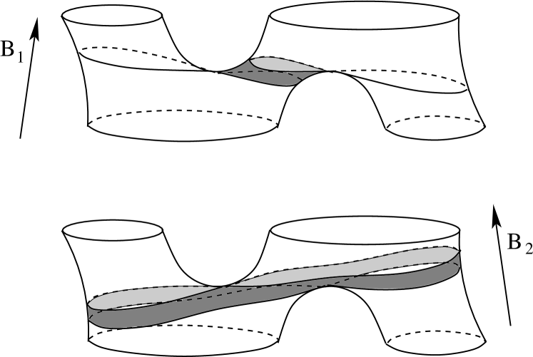
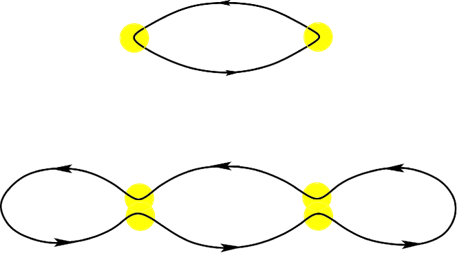
Figure 10: One of the most common reconstructions of the topological structure of system (I.1) on the Fermi surface and extreme trajectories on cylinders of small height, before and after the reconstruction (the color indicates the areas close to the singular points of system (I.1)).

The reconstruction shown in Fig. 11, cannot have central symmetry and its appearance is possible only in pairs, on the sections of the Fermi surface that transform into each other under the central inversion in the $\,{\bf p}$ - space. The cylinders of low height, both before and after the reconstruction, coincide with the one shown at the last figure of Fig. 9, and do not contain extreme area trajectories. On these cylinders, however, there are always trajectories with an extreme orbital period, the shape of which is shown at Fig. 11. When crossing the boundary of such a reconstruction, therefore, a jump occurs (a sharp change in one of the oscillatory terms) only in the picture of classical oscillations (classical cyclotron resonance, etc.).

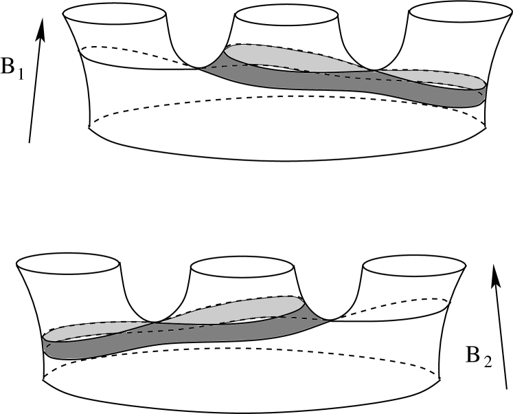
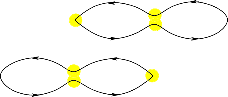
Figure 11: One of the possible reconstructions of the topological structure of system (I.1) on the Fermi surface and extremal trajectories on cylinders of low height, before and after the reconstruction (the sections close to the singular points of system (I.1) are marked with color).

Below, Fig. 12 - 21 present all the remaining topological types of ‘‘elementary’’ reconstructions of system (I.1). In addition to the shape of a reconstruction itself, Fig. 12 - 21 also show the shape of the lower and upper bases of cylinders of small height before and after the resconstruction ((a, b) and (d, e)), the shape of extreme trajectories on cylinders of small height ((c) and (f)), as well as the structure of the ‘‘cylinder of zero height’’ that appears immediately at the moment of the reconstruction (g). Strictly speaking, the above figures accurately depict the local geometry of the extreme trajectories near the above-mentioned ‘‘deceleration sections’’ on them (colored sections), as well as the topology of their connection by the remaining trajectory sections, but in other details, they can be geometrically more complicated. For the cylinders of small height under consideration, the extremal trajectories of both types are geometrically very close to each other in $\,{\bf p}$ - space (if both types of trajectories are present on the cylinder), but they can differ significantly from each other in other parameters (for example, the value of the circulation period along the trajectory). As we said above, the main goal of this work is to describe the features of oscillatory (and other) phenomena that make it possible to distinguish between different types of ‘‘elementary reconstructions’’ of the system (I.1) during their experimental observation.

Fig. 12 - 16 represent the reconstructions, during which trajectories of extreme area do not appear and do not disappear on the corresponding cylinders of small height. The extreme trajectories shown at these figures have just the smallest orbital period among all cylinder trajectories. Together with the reconstruction shown in Fig. 11, such reconstructions can be attributed to ‘‘reconstructions of the first group’’. As we said above, reconstructions of this type are distinguished by the fact that during them we have a sharp change of some of the oscillatory terms only in the picture of classical oscillations.

As it is easy to check, in all the reconstructions shown in Fig. 11 - 16, group velocities at two saddle singular points are co-directed to each other. Coming back to the description of elementary reconstructions in terms of the topology of ‘‘cylinders of zero height’’ (Fig. 7), it is easy to formulate a simple rule. Namely, for any of the types of ‘‘zero-height cylinders’’ shown in Fig. 7, trajectories of extreme area appear on the corresponding cylinders of small height (both before and after the reconstruction) if the group velocities at its singular points are directed opposite to each other.

The above rule can be easily justified using the well-known formula

$${\partial S\over\partial p_{z}}\,\,\,=\,\,\,{eB\over c}\,\oint v_{gr}^{z}\,dt$$

(where $\,t\,$ is the time of motion along the trajectory) for the area of a closed trajectory in $\,{\bf p}$ - space $\,S(p_{z})\,$. Since the singular points near the reconstruction are located at the bases of cylinders of small height, and the time of their passage tends to infinity when approaching the bases of a cylinder, this relation determines the signs of $\,\partial S/\partial p_{z}\,$ near the bases of the cylinders. As is also well known, on trajectories of the extreme area, we have the relation

$$\oint v_{gr}^{z}\,dt\,\,\,=\,\,\,0$$

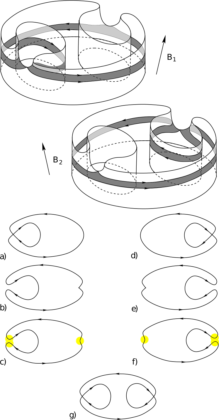
Figure 12: Reconstruction of the structure of (I.1) without central symmetry. The trajectories of the extreme area on cylinders of low height are absent both before and after the reconstruction. The trajectories of the minimum orbital period on opposite sides of the reconstruction are of the same type (electron or hole).

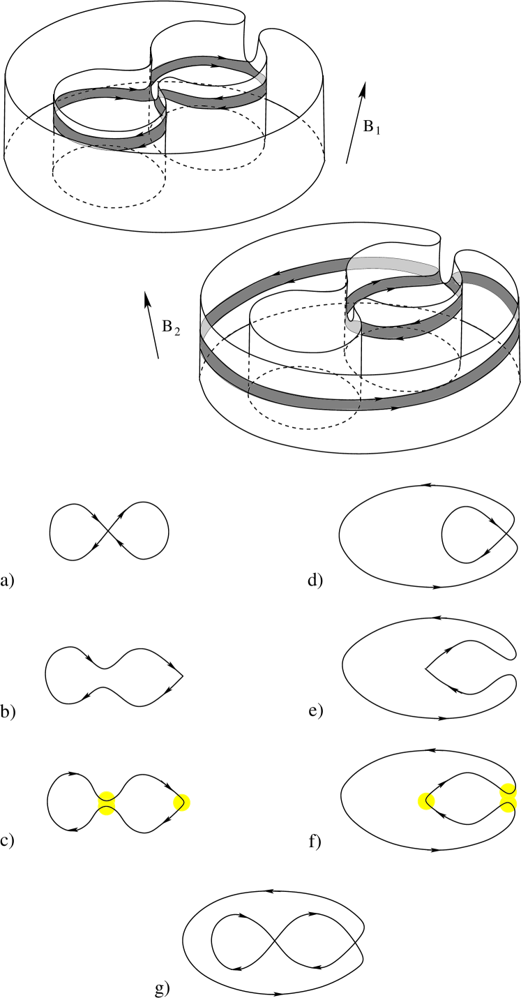
Figure 13: Reconstruction of the structure of (I.1) without central symmetry. The trajectories of the extreme area on cylinders of low height are absent both before and after the reconstruction. The trajectories of the minimum orbital period on opposite sides of the reconstruction are of different types (electronic, on the one side of the reconstruction, and hole, on the other).

It can be noted that the extreme trajectories shown at Fig. 12 - 13, as well as the trajectories shown in Fig. 11, approach the saddle singular points of the system (I.1) three times (twice to one of the singularities and once to the second). Besides that, on different sides of the reconstruction, the multiplicity of the approach of a special trajectory to each of the singular points changes (before the reconstruction, the trajectory approaches twice to one of the singular points, and after the reconstruction, to the other). Each approach to a singular point of (I.1) means the presence of a ‘‘deceleration section’’ on the corresponding part of a trajectory, which gives a finite addition to the trajectory orbital period. The corresponding addition to the orbital period grows logarithmically with decreasing angle $\,\alpha\,$ between the direction of $\,{\bf B}\,$ and the boundary of a reconstruction and for $\,\alpha\ll 1\,$ can be written as

$$\Delta T_{i}\,\,\,\simeq\,\,\,{c\over eBv^{(i)}_{gr}}\,{1\over\sqrt{G_{i}}}\,\,\ln{1\over\alpha}\,\,\,,$$

where $\,v^{(i)}_{gr}\,$ and $\,G_{i}\,$ are, respectively, the values of the group velocity and the Gaussian curvature of the Fermi surface at each of the singular points ($i=1,2$).

The total values of $\,\Delta T(\alpha)\,$ can be measured with a sufficiently accurate measurement of the orbital period in classical oscillatory phenomena and a sufficiently close approximation of the direction of $\,{\bf B}\,$ to the boundary of a reconstruction of the structure of system (I.1). It is easy to see then that when crossing the boundary, the corresponding total addition to the period of circulation along an extreme trajectory changes from the value $\,\Delta T(\alpha)=2T_{1}(\alpha)+T_{2}(\alpha)\,$ to the value $\,T_{1}(\alpha)+2T_{2}(\alpha)\,$, which distinguishes the reconstructions at Fig. 11 - 13 among all the reconstructions shown in Fig. 11 - 16. To distinguish different reconstructions in Fig. 11 - 13 a test can be used which determines the possibility of deceleration sections falling into the skin layer on each side of the boundary of a reconstruction (see OsobCycle ).

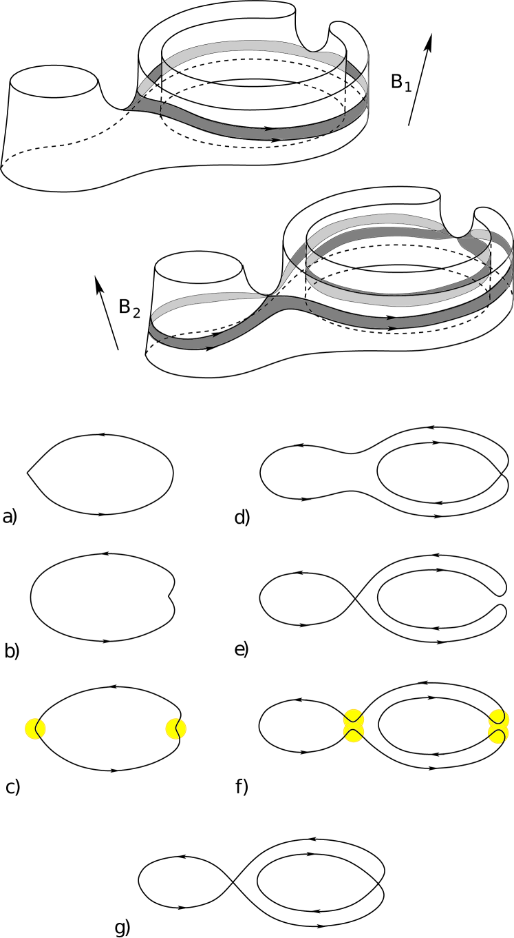
Figure 14: Reconstruction of the structure of (I.1) without central symmetry. The trajectories of the extreme area on cylinders of low height are absent both before and after the reconstruction. The trajectories of the minimum orbital period on opposite sides of the reconstruction are of the same type (electron or hole).

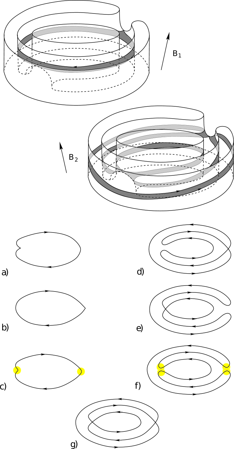
Figure 15: Reconstruction of the structure of (I.1) without central symmetry. The trajectories of the extreme area on cylinders of low height are absent both before and after the reconstruction. The trajectories of the minimum orbital period on opposite sides of the reconstruction are of different types (electronic, on the one side of the reconstruction, and hole, on the other).

For the reconstructions shown in Fig. 14 - 15, we have a different situation. Namely, now extreme trajectories have two ‘‘deceleration segments’’ on one side of a reconstruction and four ‘‘deceleration segments’’ on the other. It is easy to see that when crossing the corresponding boundary of the reconstruction the total addition to the orbital period due to the ‘‘deceleration segments’’ changes from the value $\,\Delta T(\alpha)=T_{1}(\alpha)+T_{2}(\alpha)\,$ to the value $\,2\left(T_{1}(\alpha)+T_{2}(\alpha)\right)\,$, which also makes it possible to distinguish these reconstructions among the six reconstructions of the first group.

To distinguish two reconstructions presented in Fig. 14 - 15 we can use, for example, their geometric (and topological) differences in the $\,{\bf p}$ - space, which are also transferred to the coordinate space. For example, for the trajectory shown in Fig. 14c, most of its sections can be located in the skin layer at the sample boundary both before crossing the reconstruction boundary and immediately after crossing it (we assume that the magnetic field is directed parallel to the sample boundary). For the trajectory shown in Fig. 15c, such sections do not exist, which is due to a significantly different topology of its reconstruction. The above difference for the considered reconstructions can be established, for example, by the absence or presence of a jump in the direction of $\,{\bf v}_{gr}\,$ in the section falling into the skin layer when crossing the boundary of a reconstruction. We also note here that the measurement of the corresponding direction of $\,{\bf v}_{gr}\,$ is almost always performed in the observation of the classical cyclotron resonance.

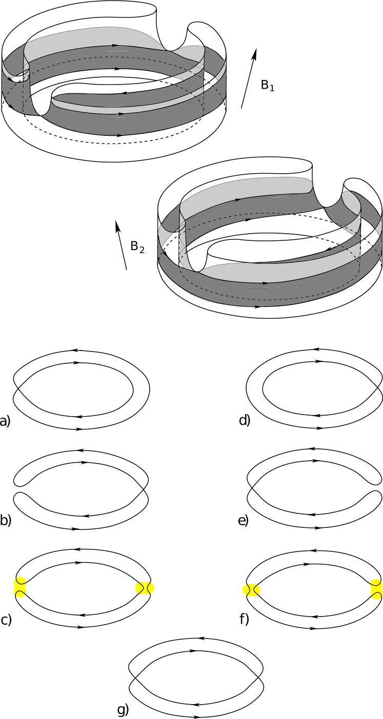
Figure 16: Reconstruction of the structure of (I.1) without central symmetry. The trajectories of the extreme area on cylinders of low height are absent both before and after the reconstruction. The trajectories of the minimum orbital period on opposite sides of the reconstruction are of the same type (electron or hole).

The reconstruction shown in Fig. 16, differs from all other reconstructions discussed above. Namely, here each of the extreme trajectories has four ‘‘deceleration sections’’ (on each side of the reconstruction boundary). When crossing the corresponding boundary of the reconstruction, the full addition to the orbital period due to the ‘‘deceleration segments’’ does not change and remains equal to $\,2\left(T_{1}(\alpha)+T_{2}(\alpha)\right)\,$. It is easy to see that this property makes it possible to unambiguously identify this reconstruction among all the reconstructions of the first group.

The remaining types of reconstructions of the system (I.1), shown in Fig. 17 - 21, on the contrary, have the property that they contain trajectories of extreme area on the cylinders of small height, both before and after the reconstruction. Together with the reconstruction shown in Fig. 10, they form the second class of reconstructions, complementing the class of reconstructions shown in Fig. 11 - 16. All these reconstructions are experimentally easily distinguishable from those of the first class, since, along with a jump in the picture of classical oscillations, they also have a jump in the picture of quantum oscillations (an abrupt replacement of some oscillation terms by others). For the experimental distinction between the reconstructions of this class, one can also use the above (and also other) features of the oscillatory picture in observing classical oscillations. But, of course, these reconstructions also differ from each other by the features of changes in the picture of quantum oscillations, which we would like to dwell on below.

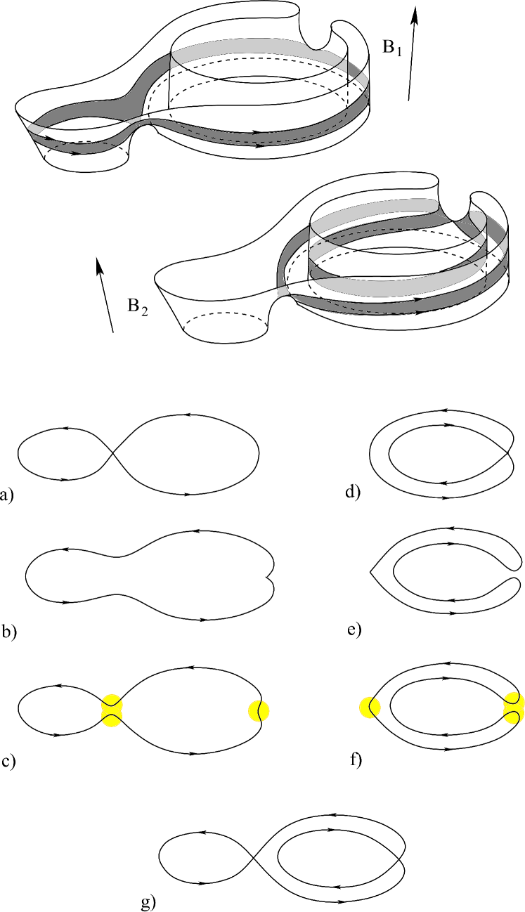
Figure 17: Reconstruction of the structure of (I.1) without central symmetry. Extreme area trajectories on low-height cylinders are present both before the reconstruction (the maximum area trajectory) and after the reconstruction (the minimum area trajectory). The area of the extreme trajectory before the reconstruction is always larger than the area of the extreme trajectory after the reconstruction. The extreme trajectories on both sides of the reconstruction are of the same (electron or hole) type.

Figure 18: Reconstruction of the structure of (I.1), which can have central symmetry. Extreme area trajectories on low-height cylinders are present both before the reconstruction (the maximum area trajectory) and after the reconstruction (the minimum area trajectory). The area of the extreme trajectory before the reconstruction is always larger than the area of the extreme trajectory after the reconstruction. The extreme trajectories on both sides of the reconstruction are of the same (electron or hole) type.

Note right away that the reconstructions, shown in Fig. 10, 17 - 18, differ from the reconstructions shown in Fig. 19 - 21. Namely, for all reconstructions shown in Fig. 10, 17 - 18, the extreme area trajectories have a minimum area on one side of a reconstruction and a maximum area on the other side. In our case, the minimality (maximality) of the trajectory area means that the trajectory area increase (decrease) when approaching the bases of the corresponding cylinder of closed trajectories for a fixed direction of $\,{\bf B}\,$. This, as we have already said, is due to the presence of singular points at the bases of such cylinders. In fact, for the same reason, the same increase (decrease) in the minimum (maximum) trajectory area (with an infinitely increasing derivative) occurs when the direction of the magnetic field approaches the boundary of a reconstruction of the structure of (I.1) (and a decrease in the height of the corresponding cylinder of closed trajectories to zero). This circumstance makes it possible to easily identify the trajectories of the minimum and maximum area described by us here, and, in particular, to distinguish experimentally the reconstructions shown in Fig. 10, 17 - 18, from the reconstructions shown in Fig. 19 - 21. As also seen from Fig. 10, 17 - 18, in all these cases, the maximum area trajectories have a larger area than the minimum area trajectories.

In addition to the above circumstance, it can also be noted that in all the reconstructions shown in Fig. 10, 17 - 18, the trajectories of the extreme area are of the same type (electron or hole) before and after the reconstruction. This circumstance can also be easily established experimentally from the behavior of quantum oscillations of transverse (Hall conductivity), which also makes it possible to distinguish these reconstructions from those shown in Fig. 19 - 21.

As for the distinguishing the reconstructions shown in Fig. 10, 17 - 18, from each other, then here, as above, we can immediately note a special feature of the reconstruction in Fig. 17, consisting in the presence of three sections of deceleration on the trajectories of cylinders of low height, both on one side and on the other side of the reconstruction. This circumstance makes it possible to immediately distinguish the reconstruction in Fig. 17 from the other two, for example, by measuring the orbital period along the trajectory when observing classical oscillations or the temperature dependence of quantum oscillations (replacing of $\,\Delta T(\alpha)=2T_{1}(\alpha)+T_{2}(\alpha)\,$ by $\,T_{1}(\alpha)+2T_{2}(\alpha)$). But, actually, this fact can be easily established also by simple observation of quantum oscillations from the behavior of the area $\,S(\alpha)\,$ of the extreme trajectory near the transition boundary, where its main dependence on $\,\alpha\,$ is determined precisely by the approache to singular points of the system (I.1). To distinguish the reconstructions shown in Fig. 10 and Fig. 18, it is possible, for example, to investigate the possibility of falling of a deceleration section into the skin layer at the sample boundary (OsobCycle ) in observing the classical cyclotron resonance (it is possible on one side of a reconstruction for the reconstruction in Fig. 10 and it is impossible for the reconstruction in Fig. 18 due to the peculiarities of the geometry of the trajectories).

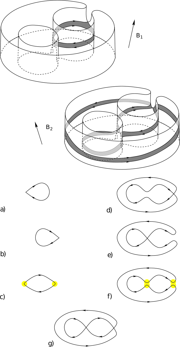
Figure 19: Reconstruction of the structure of (I.1) without central symmetry. Extreme-area trajectories on low-height cylinders are present both before the reconstruction (the trajectory of the minimum area) and after the reconstruction (the trajectory of the minimum area). The extreme trajectories on opposite sides of the reconstruction are of different types (electronic, on the one side of the reconstruction, and hole-type, on the other).

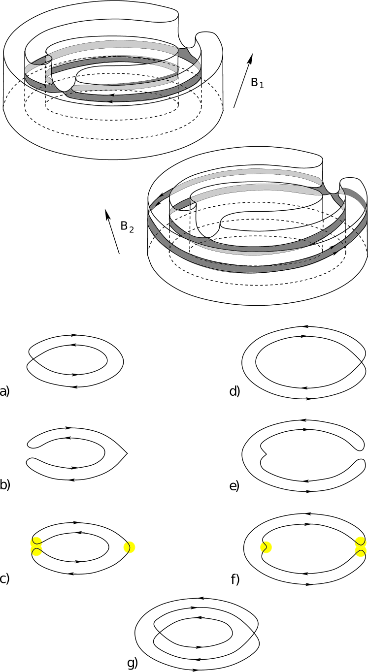
Figure 20: Reconstruction of the structure of (I.1) without central symmetry. Extreme-area trajectories on low-height cylinders are present both before the reconstruction (the trajectory of the minimum area) and after the reconstruction (the trajectory of the minimum area). The extreme trajectories on opposite sides of the reconstruction are of different types (electronic, on the one side of the reconstruction, and hole-type, on the other).

For the reconstrictions shown in Fig. 19 - 20, extreme trajectories have a minimum area on both the disappearing and arising cylinders of closed trajectories. In both of these reconstructions, the extreme trajectories have different types (electronic and hole) on opposite sides of a reconstruction. Both these circumstances can be easily established by observing quantum oscillations of various types (the De Haas - Van Alphen effect, the Shubnikov - De Haas effect) and distinguish the reconstructions in Fig. 19 - 20 from all other reconstructions. The difference between the reconstructions shown in Fig. 19 and Fig. 20, consists, for example, in the number of deceleration sections on the corresponding trajectories before and after the reconstruction. As we have already seen above, this difference can also be easily established by observing both classical and quantum oscillations.

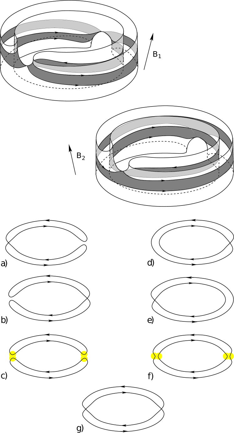
Figure 21: Reconstruction of the structure of (I.1), which can have central symmetry. Extreme area trajectories on cylinders of low height are present both before the reconstruction (a pair of trajectories of the minimum area) and after the reconstruction (one trajectory of the minimum area and one trajectory of the maximum area). A pair of extreme trajectories on one side of the reconstruction are of the same type. After the reconstruction, a pair of extreme trajectories of opposite types appear, and the type of the trajectory of a larger area coincides with the type of extreme trajectories before the reconstruction.

The reconstruction shown in Fig. 21, as it is easy to see, differs in many aspects from all the reconstructions we have considered earlier. In this reconstruction, a pair of extreme trajectories disappear and appear at once. On the one side of the reconstruction, both trajectories are of the same type (electronic or hole), while on the other side, a pair of trajectories of different types appears. This circumstance can be determined, in particular, by observing quantum oscillations of conductivity, which allows one to immediately identify this reconstruction experimentally. We also note here that the reconstruction shown in Fig. 21 may have central symmetry, which, in fact, almost always implies such symmetry in real situations.

All our considerations above was carried out without taking into account the electron spin. It is easy to see that taking into account the spin states leads to the splitting of each of the oscillatory terms into two, in accordance with the direction of the spin along or against the direction of $\,{\bf B}$. In addition, in our consideration, we also did not take into account the effect of the Berry phase, which can manifest itself in materials with no inversion center or symmetry with respect to time reversal. The appearance of nonzero Berry curvature in such materials can also lead to a number of interesting effects in the situation under consideration.

In conclusion, we would like to mention here also the phenomenon of magnetic breakdown, which can be observed in our situation. As is well known, the phenomenon of (intraband) magnetic breakdown is observed in many substances in sufficiently strong magnetic fields and, in particular, can lead to many interesting effects, arising on trajectories of system (I.1) of different geometry (see, for example etm ; Zilberman1 ; Zilberman2 ; Zilberman3 ; Azbel ; Slutskin1967 ; AlexsandradinGlazman ). Thus, it can be expected that the occurrence of a magnetic breakdown on the special extreme trajectories described above should also lead to interesting phenomena, in particular, to significantly affect the quantization of electronic levels for trajectories of the extreme area. It must be said, however, that the magnetic breakdown on the described trajectories can occur only at rather large values of $\,B\,$ and only when the direction of the magnetic field approaches the boundary of a reconstruction of the topological structure of system (I.1) very closely (see OsobCycle ). As a consequence of this, a clear picture of the corresponding effects should be observed only in very precise experiments, which make it possible to specify the directions of the magnetic field with a very high accuracy (and can be noted only as a certain blurring of the sharp changes in the oscillation picture described above in a very narrow region near the reconstruction boundary at a lower resolution). In this situation, certainly, the dependence of the picture (especially of quantum) of oscillations on the topological type of a reconstruction under conditions of developed magnetic breakdown is also of great interest.

III Conclusion

The paper considers the features of oscillatory phenomena in metals near the boundaries of reconstruction of the topological structure of the system describing the adiabatic dynamics of quasiparticles on complex Fermi surfaces. Each elementary reconstruction of such a structure is associated with a change in the picture of closed trajectories on the Fermi surface, which consists in the disappearance of some of the cylinders of closed trajectories and the appearance of new ones. Each of these reconstructions has its own topological structure, and there are a finite number of topological types of such reconstructions. The most important circumstance in each of the reconstructions is the disappearance of a part of closed trajectories with extreme values of the area or the orbital period, which leads to sharp observable changes in the picture of oscillatory phenomena during the reconstruction. The features of such changes are directly related to the geometry of disappearing and arising extreme trajectories, which is determined by the topological type of a reconstruction. The paper presents a detailed comparison of the features of the change in the picture of classical and quantum oscillations at the moment of a reconstruction with its topological type and proposes methods for identifying topological types based on these features. The proposed methods, in our opinion, can be rather useful in studying the geometry of complex Fermi surfaces using classical or quantum oscillations in strong magnetic fields.

This work is supported by the Russian Science Foundation under grant 21-11-00331.

References

- (1) I.M.Lifshitz, M.Ya.Azbel, M.I.Kaganov. The Theory of Galvanomagnetic Effects in Metals., Sov. Phys. JETP 4:1, 41-53 (1957).
- (2) I.M. Lifshitz, V.G. Peschansky., Galvanomagnetic characteristics of metals with open Fermi surfaces., Sov. Phys. JETP 8:5, 875-883 (1959).
- (3) I.M. Lifshitz, V.G. Peschansky., Galvanomagnetic characteristics of metals with open Fermi surfaces. II., Sov. Phys. JETP 11:1, 131-141 (1960).
- (4) I.M. Lifshitz, M.I. Kaganov., Some problems of the electron theory of metals I. Classical and quantum mechanics of electrons in metals., Sov. Phys. Usp. 2:6 (1960), 831-835.
- (5) I.M. Lifshitz, M.I. Kaganov., Some problems of the electron theory of metals II. Statistical mechanics and thermodynamics of electrons in metals., Sov. Phys. Usp. 5:6 (1963), 878-907.
- (6) I.M. Lifshitz, M.I. Kaganov., Some problems of the electron theory of metals III. Kinetic properties of electrons in metals., Sov. Phys. Usp. 8:6 (1966), 805-851.
- (7) I.M. Lifshitz, M.Ya. Azbel, M.I. Kaganov., Electron Theory of Metals. Moscow, Nauka, 1971. Translated: New York: Consultants Bureau, 1973.
- (8) M.I. Kaganov, V.G. Peschansky., Galvano-magnetic phenomena today and forty years ago., Physics Reports 372 (2002), 445-487.
- (9) S.P. Novikov., The Hamiltonian formalism and a many-valued analogue of Morse theory., Russian Math. Surveys 37 (5) (1982), 1-56.
- (10) A.V. Zorich., A problem of Novikov on the semiclassical motion of an electron in a uniform almost rational magnetic field., Russian Math. Surveys 39 (5) (1984), 287-288.
- (11) I.A. Dynnikov., Proof of S.P. Novikov’s conjecture for the case of small perturbations of rational magnetic fields., Russian Math. Surveys 47 (3) (1992), 172-173.
- (12) I.A. Dynnikov., Proof of S.P. Novikov’s conjecture on the semiclassical motion of an electron., Math. Notes 53:5 (1993), 495-501.
- (13) A.V. Zorich., Proc. ‘‘Geometric Study of Foliations’’., (Tokyo, November 1993) / ed. T.Mizutani et al. Singapore: World Scientific, 479-498 (1994).
- (14) I.A. Dynnikov., Surfaces in 3-torus: geometry of plane sections., Proc. of ECM2, BuDA, 1996.
- (15) I.A. Dynnikov., Semiclassical motion of the electron. A proof of the Novikov conjecture in general position and counterexamples., Solitons, geometry, and topology: on the crossroad, Amer. Math. Soc. Transl. Ser. 2, 179, Amer. Math. Soc., Providence, RI, 1997, 45-73.
- (16) I.A. Dynnikov., The geometry of stability regions in Novikov’s problem on the semiclassical motion of an electron., Russian Math. Surveys 54:1 (1999), 21-59.
- (17) S.P. Novikov, A.Y. Maltsev., Topological quantum characteristics observed in the investigation of the conductivity in normal metals., JETP Letters 63 (10) (1996), 855-860.
- (18) S.P. Novikov, A.Y. Maltsev., Topological phenomena in normal metals., Physics-Uspekhi 41:3 (1998), 231-239.
- (19) S.P. Tsarev. Private communication. (1992-93).
- (20) A.Y. Maltsev., Anomalous behavior of the electrical conductivity tensor in strong magnetic fields., J. Exp. Theor. Phys. 85 (5) (1997), 934-942.
- (21) A.Ya. Maltsev, S.P. Novikov., The theory of closed 1-forms, levels of quasiperiodic functions and transport phenomena in electron systems., Proceedings of the Steklov Institute of Mathematics, 2018, Vol. 302, pp. 279–297
- (22) A.Ya. Maltsev, S.P. Novikov., Quasiperiodic functions and Dynamical Systems in Quantum Solid State Physics., Bulletin of Braz. Math. Society, New Series 34:1 (2003), 171-210.
- (23) A.Ya. Maltsev, S.P. Novikov., Dynamical Systems, Topology and Conductivity in Normal Metals in strong magnetic fields., Journal of Statistical Physics 115:(1-2) (2004), 31-46.
- (24) A.Ya. Maltsev, S.P. Novikov., Topological integrability, classical and quantum chaos, and the theory of dynamical systems in the physics of condensed matter., Russian Mathematical Surveys 74(1) (2019), 141-173
- (25) S.P. Novikov, R. De Leo, I.A. Dynnikov, A.Ya. Maltsev., Theory of Dynamical Systems and Transport Phenomena in Normal Metals., J. Exp. Theor. Phys. 129:4 (2019), 710-721
- (26) A.Ya. Maltsev., Reconstructions of the Electron Dynamics in Magnetic Field and the Geometry of Complex Fermi Surfaces., J. Exp. Theor. Phys. 131:6 (2020), 988-1020
- (27) C. Kittel., Quantum Theory of Solids., Wiley, 1963.
- (28) A.A. Abrikosov., Fundamentals of the Theory of Metals., Elsevier Science & Technology, Oxford, United Kingdom, 1988.
- (29) I. Lifshitz and A. Kosevich, Dokl. Akad. Nauk SSSR 96 (1954), 963-966
- (30) G.E. Zil’berman, Behavior of an Electron in a Periodic Electric and a Uniform Magnetic Field, Soviet Physics JETP 5:2 (1957), 208-215
- (31) G.E. Zil’berman, Electron in a Periodic Electric and Homogenous Magnetic Field, II., Soviet Physics JETP 6:2 (1958), 299-306
- (32) G.E. Zil’berman, Motion of Electron along Self-Intersecting Trajectories., Soviet Physics JETP 7:3 (1958), 513-514
- (33) M.Ia. Azbel, Quasiclassical Quantization in the Neighborhood of Singular Classical Trajectories., Soviet Physics JETP 12:5 (1961), 891-897
- (34) A.A. Slutskin, Dynamics of Conduction Electrons under Magnetic Breakdown Conditions, Soviet Physics JETP 26:2 (1968), 474-482
- (35) A. Alexandradinata and Leonid Glazman., Semiclassical theory of Landau levels and magnetic breakdown in topological metals., Phys. Rev. B 97 (2018), 144422