Collectively pair-driven-dissipative bosonic arrays:
exotic and self-oscillatory condensates

Abstract

Modern quantum platforms such as superconducting circuits provide exciting opportunities for the experimental exploration of driven-dissipative many-body systems in unconventional regimes. One of such regimes occurs in bosonic systems, where nowadays one can induce driving and dissipation through pairs of excitations, rather than the conventional single-excitation or linear processes. Moreover, modern platforms can be driven in a way in which the modes of the bosonic array decay collectively rather than locally, such that the pairs of excitations recorded by the environment do not come from a specific lattice site, but by a coherent superposition of all sites. In this work we analyze the superfluid phases accessible to bosonic arrays subject to these novel mechanisms more characteristic of quantum optics, which we prove to lead to remarkable spatiotemporal properties beyond the traditional scope of pattern formation in condensed-matter systems or nonlinear optics alone. In particular, we show that, even in the presence of residual local loss, the system is stabilized into an exotic state with bosons condensed along the modes of a closed manifold in Fourier space, with a distribution of the population among these Fourier modes that can be controlled via a weak bias (linear) drive. This gives access to a plethora of different patterns, ranging from periodic and quasi-periodic ones with tunable spatial wavelength, to homogeneously-populated closed-Fourier-manifold condensates that are thought to play an important role in some open problems of condensed-matter physics. Moreover, we show that when any residual local linear dissipation is balanced with pumping, new constants of motion emerge that can force the superfluid to oscillate in time, similarly to the mechanism behind the recently discovered superfluid time crystals. We propose specific experimental implementations with which this rich and unusual spatiotemporal superfluid behavior can be explored.

I Introduction

In the last couple of decades we have been able to explore quantum many-body phenomena with a level of control never thought accessible before. This has been possible thanks to the development of many clean and controllable experimental platforms that act as so-called quantum simulators (Cirac and Zoller, 2012; Bloch et al., 2012; Blatt and Roos, 2012; Aspuru-Guzik and Walther, 2012; Houck et al., 2012; Altman et al., 2021), such as trapped ultracold atoms (Bloch et al., 2008; Jaksch and Zoller, 2005; Dutta et al., 2015). These are well isolated devices that essentially behave as closed quantum systems where a variety of many-body bosonic (Schweizer et al., 2019; Wintersperger et al., 2020), fermionic (M. et al., 2021; Koepsell et al., 2020; Sompet et al., 2021; Boll et al., 2016; Hilker et al., 2017; Hachmann et al., 2021; Greif et al., 2015), or spin Hamiltonians (Zeiher et al., 2017; Fukuhara et al., 2013a, b; Ebadi et al., 2021; Jepsen et al., 2020) can be engineered. In combination with very flexible measurement techniques giving access to a wide range of observables, these systems have allowed the observation of many physical phenomena ranging from the already classic insulator-superfluid phase transition of the Bose-Hubbard model (Greiner et al., 2002), to supersolidity (Léonard et al., 2017a; Li et al., 2017; Léonard et al., 2017b), topological effects (Hilker et al., 2017; Sompet et al., 2021; Lohse et al., 2016; Kennedy et al., 2015; Semeghini et al., 2021), or many-body localization (Schreiber et al., 2015; yoon Choi et al., 2016; Lüschen et al., 2017; Abanin et al., 2019; Kohlert et al., 2019) and other routes to the breaking of thermalization (Kohlert et al., 2021). By coupling these systems to the optical modes of a laser-driven lossy cavity (Black et al., 2003; Ritsch et al., 2013; Brennecke et al., 2013; Klinder et al., 2015a, b; Zupancic et al., 2019; Ferri et al., 2021; Li et al., 2021), we have even been able to access the domain of driven-dissipative many-body physics (Sieberer et al., 2016). These scenarios are intrinsically out of thermodynamic equilibrium, and the competition between driving, dissipation, and interactions can stabilize the system into asymptotic states that can be inaccessible to closed systems, for example time crystals (Keßler et al., 2020, 2021). This so-called dissipative-state preparation (Verstraete et al., 2009) has provided further motivation for the development of controlled driven-dissipative experimental platforms. In the bosonic realm which occupies our current work, perhaps the best explored platforms are exciton polaritons in semicondutor microcavities (Carusotto and Ciuti, 2013; Boulier et al., 2020; Solnyshkov et al., 2020), among other photonic platforms (Bloch et al., 2021; Ozawa et al., 2019), where spontaneous spatial coherence in the form of a wide variety of patterns, as well topological phenomena has been reported by now.

In recent years, another experimental platform is taking over as a leading candidate for the implementation of driven-dissipative bosonic many-body scenarios (Ma et al., 2019; Schmidt and Koch, 2013; Houck et al., 2012), the so-called superconducting circuits (Blais et al., 2021; Krantz et al., 2019; Gu et al., 2017). These solid-state systems are extremely flexible not only in terms of geometric design, but also in terms of the type of processes that one can engineer on them. Currently, 2D arrays with up to 66 bosonic modes have been developed and used to explore quantum advantage (F. Arute et al., 2019; Wu et al., 2021; Q. Zhu et al., ), discrete time crystals (X. Mi et al., ; X. Zhang et al., ), localization and thermalization (Chen et al., 2021; Gong et al., 2021; Ye et al., 2019; Xu et al., 2018), as well as quantum walks and topological phenomena (K. J. Satzinger et al., ; M. Gong et al., 2021; Owens et al., 2018; Flurin et al., 2017). Here, the intrinsic energies of the bosonic modes are on the microwave domain, where we are able to synthesize coherent drives with arbitrary spectral profiles. In addition, the tunneling rates between the modes can be controlled in real time and can be made complex (artificial gauge fields). Moreover, interactions between the bosonic modes can be engineered via the four-wave mixing occurring at the Josephson junctions that are naturally integrated in these platforms, which also allow for the implementation of pair driving and dissipation (Leghtas et al., 2015; Touzard et al., 2018; Lescanne et al., 2020; Ma et al., 2021). There are well-known processes in quantum optics, but very unconventional in the many-body models derived from condensed-matter physics.

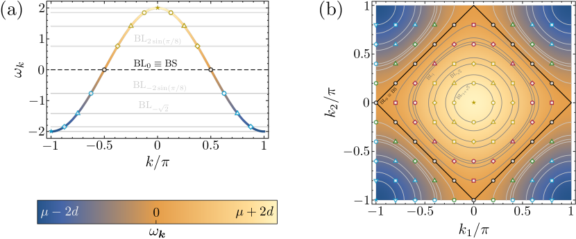
Figure 1: Dispersion relation $\omega_{\bm{k}}$ in 1D (a) and 2D (b), that is, $d=1$ and $2$, respectively. We have chosen $\mu=0$ with $L=16$ for the 1D case (a) and $L=10$ for 2D (b). We denote by $k$ and $\bm{k}=(k_{1},k_{2})$ the wave vectors in 1D and 2D, respectively. We also show the legend for the color scale denoting the values of $\omega_{\bm{k}}$, which range between $\mu-2d$ (darkest blue) and $\mu+2d$ (lighter yellow). Markers of the same type and color correspond to wave vectors $\bm{k}$ lying at the same ‘Bose level’ $\mathrm{BL}_{\beta}$, that is, $\omega_{\bm{k}}=\beta$. The Bose level $\mathrm{BL}_{0}$ plays a central role in our work, since it contains the most divergent modes, which eventually form the bulk of the asymptotic state; we dub it the ‘Bose surface’ or $\mathrm{BS}$ (Wang et al., 2020), and highlight it thick black. Note that the Bose levels $\mathrm{BL}_{\mu\pm 2d}$ contain a single wave vector in all dimensions, for which we have used a star marker. The rest of Bose levels contain multiple wave vectors, only two in 1D, but many in 2D, eventually forming a closed curve with an infinite number points in the thermodynamic limit $L\rightarrow\infty$, represented by the contours in (b) for the specific values of $\beta$ appearing for $L=10$.

This toolbox makes superconducting-circuit arrays a theoretician’s dream for the implementation of interesting and unconventional models beyond traditional condensed-matter systems. With this motivation, in this work we study the superfluid phases that emerge in a bosonic array in the presence of pair driving and the corresponding pair loss, showing that these lead to incredibly rich spatiotemporal phenomena. In particular, we consider (and propose a generic implementation for) the case in which pair loss occurs through a collective channel, i.e., the information about which array site the pair came from is washed off before decaying into the environment. In such case, even in the presence of additional linear local loss, we show that it is possible to stabilize the superfluid into an exotic one with bosons condensed on the modes of a closed manifold in Fourier space (which we also recently predicted to appear with local pair loss (Wang et al., 2020), but only when the chemical potential and the linear decay are fine-tuned to zero exactly, which is too demanding under realistic experimental conditions). Moreover, at difference with (Wang et al., 2020), the distribution of population along the ring can be controlled by biasing the system via the initial conditions or a weak external drive. This opens the possibility of stabilizing a plethora of patterns, from periodic and quasi-periodic ones with tunable spatial wavelength, to homogeneously-populated closed Fourier manifolds. The latter have been conjectured to play a fundamental role in several open problems in condensed-matter physics such as high-$T_{\text{c}}$ superconductivity (Jiang et al., 2019), frustrated magnetism (Sedrakyan et al., 2015), and interacting problems with spin-orbit coupling (Wu et al., 2011; Gopalakrishnan et al., 2011). Our proposal then opens the way to the systematic study of such broad type of patterns under controlled experimental conditions.

In addition, when the local linear loss is balanced by incoherent pumping (Navarrete-Benlloch et al., 2014; Marthaler et al., 2011; Grajcar et al., 2008; Astafiev et al., 2007), we show that new constants of motion emerge in the system, which lead to asymptotic self-oscillatory states. This behavior is reminiscent of superfluid time crystals (Autti et al., 2018, 2021, ), where the conservation of the particle number, together with a non-zero chemical potential induce robust temporal oscillations in the macroscopic wave function of the condensed fraction.

Our results indicate that the combination of quantum-optical processes and condensed-matter models allows one to go beyond the paradigm accessible to these disciplines separately.

The paper is organized as follows. In the next two sections we introduce the model, equations, and main concepts that we use to unravel the behavior of the system. In Section IV we present the results found in the absence of local linear loss, whose effect we analyze in Section V. Finally, in Section VI we explain how to implement our model with state-of-the-art superconducting-circuit devices.

II Model

We consider $N$ bosonic modes with annihilation operators $\hat{a}_{\bm{j}}$ arranged in the nodes of a $d$-dimensional square array, so that the mode indices are parametrized as $\bm{j}=(j_{1},...,j_{d})$, with $j_{n}\in\{1,2,...,L\}$ and $N=L^{d}$. The operators satisfy canonical commutation relations, $[\hat{a}_{\bm{j}},\hat{a}_{\bm{l}}]=0$ and $[\hat{a}_{\bm{j}},\hat{a}_{\bm{l}}^{\dagger}]=\delta_{\bm{jl}}$. Apart from the standard chemical potential and nearest-neighbor hopping terms of the Bose-Hubbard model, we consider pair-driving in the Hamiltonian that breaks particle-number conservation, but still keeping a $Z_{2}$ symmetry $\hat{a}_{\bm{j}}\rightarrow-\hat{a}_{\bm{j}}\,\forall\bm{j}$, see Eq. (2a). Such driving must be necessarily accompanied by pair dissipation. Here we study the case in which the environment used for driving is common to all modes, such that a single collective jump operator $\sum_{\bm{j}}\hat{a}_{\bm{j}}^{2}$ effects the decay process. In contrast to local decay, we will show that such type of decay allows for a much richer, flexible, and controllable spatiotemporal phenomena. In addition, we consider the possibility of having local decay, typically unavoidable in real setups, as well as incoherent pumping to compensate it. We will discuss later plausible implementations of this model in the context of superconducting-circuit arrays. The master equation describing the evolution of the state of the system $\hat{\rho}$ reads

$$\partial_{t}\hat{\rho}=-\mathrm{i}\biggl{[}\frac{\hat{H}}{\hbar},\hat{\rho}\biggr{]} +\frac{\gamma}{2N}\mathcal{D}_{\sum_{\bm{j}}\hat{a}_{\bm{j}}^{2}}\left[\hat{\rho}\right]$$ (1)

$$+\sum_{\bm{j}}\left(\gamma_{0}\mathcal{D}_{\hat{a}_{\bm{j}}}\left[\hat{\rho}\right]+\Gamma\mathcal{D}_{\hat{a}_{\bm{j}}^{\dagger}}\left[\hat{\rho}\right]\right),$$

where

$$\frac{\hat{H}}{\hbar}=\sum_{\bm{j}}\left[-\mu\hat{a}_{\bm{j}}^{\dagger}\hat{a}_{\bm{j}}+\frac{\varepsilon}{2}\left(\hat{a}_{\bm{j}}^{2}+\hat{a}_{\bm{j}}^{\dagger}{}^{2}\right)\right]-J\sum_{\langle\bm{jl}\rangle}\hat{a}_{\bm{j}}\hat{a}_{\bm{l}}^{\dagger},$$ (2a)

$$\mathcal{D}_{A}[\hat{\rho}]=2\hat{A}\hat{\rho}\hat{A}^{\dagger}-\hat{A}^{\dagger}\hat{A}\hat{\rho}-\hat{\rho}\hat{A}^{\dagger}\hat{A}.$$ (2b)

Here $\mu$ plays the role of a chemical potential (corresponding in the implementation to the detuning of a driving field, which is fully tunable, as we will see later), $\varepsilon$ is the pair-injection rate, and $J$ is the hopping rate, the $\langle\bm{jl}\rangle$ symbol denoting that the sum runs only over nearest neighbors. As for the parameters in the incoherent terms, all assumed of the Lindblad form (2b) under the standard Born-Markov conditions satisfied by most quantum-optical systems, $\gamma_{0}$ is the local linear decay rate, $\Gamma$ is the pumping rate, and $\gamma/2N$ is the collective nonlinear decay rate, which is normalized by $N$ in order to make all terms in the master equation extensive. All the parameters are taken positive except for $\mu$, which we allow to take on negative values, as this is naturally the case in experiments (the driving can be red-detuned or blue-detuned with respect to resonance).

We assume to be deep in the superfluid phase, where the $Z_{2}$ symmetry is spontaneously broken and the system is well described by a coherent-state ansatz with amplitudes $\langle\hat{a}_{\bm{j}}\rangle=\psi_{\bm{j}}\in\mathbb{C}$ (Svistunov et al., 2015). Let us remark that, while one might argue that driving and dissipation would prevent the system to reach true superfluidity, it is by now well established that this is not the case. In particular, both theory/simulations (Kinsler and Drummond, 1991; Navarrete-Benlloch et al., 2017; Iemini et al., 2018) and experiments (Carusotto and Ciuti, 2013; Boulier et al., 2020; Solnyshkov et al., 2020) show that it takes an infinite time to tunnel in between the symmetry-breaking coherent states in the thermodynamic limit for sufficiently weak interactions or nonlinearity, and hence such superfluid states are true robust asymptotic states accessible to the system. As shown in Appendix A, in this regime the master equation (1) is then translated into a set of nonlinear differential equations for the coherent amplitudes (generalized Gross-Pitaevskii or GP equations). Furthermore, we can set two parameters to one, say $J=1$ and $\gamma/N=1$, which is equivalent to normalizing all rates to $J$, time to $J^{-1}$, and the amplitudes $\psi_{\bm{j}}$ to $\sqrt{NJ/\gamma}$, as detailed in Appendix A. The resulting equations read

$$\dot{\psi}_{\bm{j}}=\left(\mathrm{i}\mu-\kappa\right)\psi_{\bm{j}}-\left(\mathrm{i}\varepsilon+\sum_{\bm{l}}\psi_{\bm{l}}^{2}\right)\psi_{\bm{j}}^{*}+\mathrm{i}\sum_{\left<\bm{l}\right>_{\bm{j}}}\psi_{\bm{l}},$$ (3)

where $\left<\bm{l}\right>_{\bm{j}}$ denotes that the sum extends only over nearest neighbors of $\bm{j}$, and we have defined the linear decay rate $\kappa=\gamma_{0}-\Gamma$, which combines the local damping and pumping, and is assumed to be positive or zero in the following (that is to say, pumping can only compensate damping, but not go above it).

Owed to the translational invariance of the problem (we assume periodic boundary conditions for simplicity), it is more convenient to work in the Fourier basis $\alpha_{\bm{k}}=\frac{1}{\sqrt{N}}\sum_{\bm{j}}e^{\mathrm{i}\bm{k}\cdot\bm{j}}\psi_{\bm{j}}$, with $\bm{k}=(k_{1},...,k_{d})$ the Fourier wave vector, whose components take on values

$$\frac{k_{n}L}{2\pi}\in\left\{-\left\lfloor\frac{L}{2}\right\rfloor,-\left\lfloor\frac{L}{2}\right\rfloor+1,...,-\left\lfloor\frac{L}{2}\right\rfloor+L-1\right\},$$ (4)

working in the first Brillouin zone, meaning that the Fourier indices become continuous $k_{n}\in[-\pi,\pi[$ in the thermodynamic limit $L\rightarrow\infty$. Transforming the GP equations (3) to Fourier space, we obtain

$$\dot{\alpha}_{\bm{k}}=\left(\mathrm{i}\omega_{\bm{k}}-\kappa\right)\alpha_{\bm{k}}-\left(\mathrm{\mathrm{i}}\varepsilon+\sum_{\bm{q}}\alpha_{\bm{q}}\alpha_{-\bm{q}}\right)\alpha_{-\bm{k}}^{*},$$ (5)

where

$$\omega_{\bm{k}}=\mu+2\sum_{n=1}^{d}\cos k_{n},$$ (6)

is the (negative of the) dispersion relation, which we represent Fig. 1 for dimensions $d=1$ and $2$. Interestingly, these GP equations are invariant under several transformations, most notably continuous shifts of the relative phase between each $\pm\bm{k}$ pair, continuous time translations, and the exchange of any pairs $\pm\bm{k}$ with the same value of the dispersion relation (which is also a continuous symmetry in the thermodynamic limit for $d>1$). This implies that any symmetry-breaking solution will be accompanied by the corresponding Goldstone modes whose fluctuations can make the solutions change without opposition, as we will see later.

This is the set of equations that we focus on in this work. Let us remark that, while we have performed extensive numerical simulations of the equations, most of the results are understood from analytical or semi-analytical arguments, as we explain below. Before proceeding, though, let us introduce a few concepts that will turn out to be very useful for the analysis of the asymptotic states.

III Bose levels and
collective equations

Consider the dissipativeless limit of the model ($\kappa=0=\gamma$), where the GP equations simply read $\dot{\alpha}_{\bm{k}}=\mathrm{i}\omega_{\bm{k}}\alpha_{\bm{k}}-\mathrm{i}\varepsilon\alpha_{-\bm{k}}^{*}$. When $\varepsilon<|\omega_{\bm{k}}|$, the amplitudes $\alpha_{\bm{k}}(t)$ remain bounded and oscillate in time at frequency $\sqrt{\omega_{\bm{k}}^{2}-\varepsilon^{2}}$. In contrast, when $\varepsilon>|\omega_{\bm{k}}|$ these frequencies become imaginary, meaning that the amplitudes diverge exponentially with time at rate $\sqrt{\varepsilon^{2}-\omega_{\bm{k}}^{2}}$. One then expects that the modes with largest divergence rate will dominate the long-term dynamics of the full problem, including dissipation. When the chemical potential satisfies $|\mu|<2d$ (which we assume in the following), the most divergent modes are characterized by $\omega_{\bm{k}}=0$, and define the bosonic analog of the Fermi surface, which we dubbed the ‘Bose surface’ in (Wang et al., 2020) (highlighted thick black in Fig. 1). In general, since Fourier modes with the same value of $\omega_{\bm{k}}$ have the same divergence rate or oscillation frequency, it is convenient to group them into what we will call ‘Bose levels’ (see Fig. 1). Let us denote by $\{\beta\}$ the collection of distinct values that $\omega_{\bm{k}}$ can take, which take continuously over the whole interval $[\mu-2d,\mu+2d]$ in the thermodynamic limit, but otherwise form a discrete set within that interval. We define Bose level $\beta$, and abbreviate it by $\mathrm{BL}_{\beta}$, as the set of Fourier modes $\bm{k}$ for which $\omega_{\bm{k}}=\beta$. The particular Bose level with $\beta=0$, $\mathrm{BL}_{0}$, is then the Bose surface (abbreviated $\mathrm{BS}$), containing the most divergent modes. Note that the Bose levels with $\beta=\mu\pm 2d$ lying at the center and the edge of the Brillouin zone contain a single mode, respectively, $\bm{k}=(0,...,0)$ or $(\pi,...,\pi)$; none of these two Bose levels are the Bose surface, because of our previous $|\mu|<2d$ assumption. All other Bose levels form a closed curve ($d=2$) or surface ($d=3$) in Fourier space, and are constituted by multiple $\pm\bm{k}$ pairs with opposite wave vector, see Fig. 1(b). This does not hold in one dimension ($d=1$), for which Bose levels are formed by a single pair of opposite wave-vector modes, see Fig. 1(a).

It is interesting to define the collective Bose-level variables

$$\sum_{\bm{k}\in\mathrm{BL}_{\beta}}\alpha_{\bm{k}}\alpha_{\bm{-k}} \equiv s_{\beta},$$ (7a)

$$\sum_{\bm{k}\in\mathrm{BL}_{\beta}}\left|\alpha_{\bm{k}}\right|^{2} \equiv n_{\beta},$$ (7b)

which wash off the details about each specific mode of $\mathrm{BL}_{\beta}$, but describe the excitation of the level as a whole. In particular, note that $n_{\beta}$ provides the total population at $\mathrm{BL}_{\beta}$. It is simple using the GP equation (5) to show that the collection of these Bose-level variables evolve according to a closed set of equations that reads

$$\dot{s}_{\beta} =2(\mathrm{i}\beta-\kappa)s_{\beta}-2n_{\beta}\Bigl{(}\mathrm{i}\varepsilon+\sum_{\beta^{\prime}}s_{\beta^{\prime}}\Bigr{)},$$ (8a)

$$\dot{n}_{\beta} =-2\kappa n_{\beta}-\Bigl{[}s_{\beta}^{*}\Bigl{(}\mathrm{i}\varepsilon+\sum_{\beta^{\prime}}s_{\beta^{\prime}}\Bigr{)}+\mathrm{c.c.}\Bigr{]},$$ (8b)

where the sums extend over all Bose levels. We dub these the Bose-level equations of motion. They will be very useful when studying the types of asymptotic states that the system can reach, which we pass now to discuss first for $\kappa=0$ in the next section, and then considering the effect of linear dissipation $\kappa\neq 0$ one section later.

IV Purely nonlinear dissipation:
constants of motion
and oscillatory states

In this section we analyze the stationary solutions ($\dot{\alpha}_{\bm{k}}=0$) of the GP equations in the absence of linear dissipation ($\kappa=0$). First, note that the trivial state $\alpha_{\bm{k}}=0$ exists but it’s unstable by assumption: since we assume that the $\omega_{\bm{k}}=0$ Bose surface exists, even an infinitesimal driving rate $\varepsilon$ will make fluctuations increase exponentially towards a nontrivial solution (see Appendix E.1). On the other hand, we prove in Appendix B that stationary solutions can populate only modes with the same $|\omega_{\bm{k}}|$. Hence, stationary solutions only populate at most two Bose levels, those with opposite value of the dispersion, say, $\omega_{\bm{k}}=\pm\Omega$.

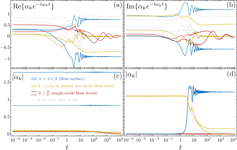
Figure 2: Numerical simulation of the time evolution of $\alpha_{k}(t)$ from the Gross-Pitaevskii equations (5) in 1D ($d=1$) for size $L=12$. Here we consider no local damping ($\kappa=0$), taking $\varepsilon=3$ and $\mu=0$, but the same behavior is found for other parameters, sizes, and dimensions. We highlight the modes $k=\pm\pi/2$ at the Bose surface $\omega_{\pi/2}=0$ (blue), the modes $k=0$ and $\pi$ at the edge of the dispersion relation $\omega_{0,\pi}=\mu\pm 2$ (red), and the modes $k=\pm 5\pi/6$ at the lowest nontrivial Bose level (yellow). The thinner grey lines correspond to the rest of the modes. (a) and (b) show the real and imaginary parts of $\alpha_{k}e^{-\mathrm{i}\omega_{k}t}$ starting from random initial conditions. Note that the lines converge to steady values, showing that the $k$ modes oscillate as $e^{\mathrm{i}\omega_{k}t}$ in the asymptotic state. Most population flows into the modes at the Bose surface, but one mode of each $\pm k$ pair at other Bose levels remains populated, as required by the existence of the constants of motion that we discuss in the main text. The population of modes $k=0$ and $\pi$ vanishes asymptotically, but note that their equilibration rate can be much slower than that of the other Bose levels. (c) shows the populations $|\alpha_{k}|$ starting from a fully random perturbation ($\leq$5%) around the stationary solution (9) with only the Bose-surface modes excited, specifically the imbalanced configuration $\alpha_{\pi/2}=\sqrt{\varepsilon}e^{\mathrm{i}\pi/4}=2\alpha_{-\pi/2}$. The simulations agree with these stationary solutions being (marginally) stable. In contrast, (d) starts from a random perturbation ($\leq$1%) around a stationary solution (10) with only the $k=\pm 5\pi/6$ modes excited, and shows that such stationary solutions are very unstable. All these numerical simulations (and the many more we have conducted, including 2D and 3D situations) agree with the analytical results that we work out in the main text.

When the populated level is the Bose surface, that is, when all $\alpha_{\bm{k}\notin\mathrm{BS}}=0$, we can set $\omega_{\bm{k}}=0$ in the GP equation (5) and obtain a set of stationary solutions constrained only by the condition

$$\sum_{\bm{k}\in\mathrm{BS}}\alpha_{\bm{k}}\alpha_{\bm{-k}}=-\mathrm{i}\varepsilon.$$ (9)

Any configuration of amplitudes $\alpha_{\bm{k}\in\mathrm{BS}}$ satisfying this condition is a valid stationary solution. We comment on the stability of these configurations shortly, but let us anticipate that they are marginally stable, meaning that fluctuations around them do not grow, but might not be damped either, see Fig. 2(c). This is owed to Goldstone’s theorem applied to the continuous symmetries of the GP equations that are spontaneously broken by the stationary solution, as well as to the existence of extra constants of motion that we introduce below.

Let us consider now stationary configurations populating an arbitrary pair of Bose levels with $\omega_{\bm{k}}=\pm\Omega$, which we denote here by $\mathrm{BL}_{\pm}\neq\mathrm{BS}$, so that $\alpha_{\bm{k}\notin\mathrm{BL_{\pm}}}=0$. In contrast to the Bose-surface solutions, we will prove later and show in Fig. 2(d) that these ones are unstable. Nevertheless, it is still instructive to consider and understand them, as they will allow us to introduce some useful concepts, as well as provide insight into the privileged role of the Bose surface. In Appendix B we discuss this type of stationary configurations in detail. They are constrained by two conditions

$$|n_{+}-n_{-}| =\sqrt{\varepsilon^{2}-\Omega^{2}},$$ (10a)

$$\alpha_{\bm{-k}\in\mathrm{BL}_{\pm}} =-\mathrm{i}e^{\mathrm{i}\varphi_{\pm}}\alpha_{\bm{k}}^{*},$$ (10b)

where $\varphi_{\pm}=\arg\left\{\pm(n_{+}-n_{-}+\mathrm{i}\Omega)\right\}$ is a phase common to all $\bm{k}$ modes within the same Bose level. The first thing to note is that only Bose levels for which $\varepsilon>|\Omega|$ can be excited as stationary solutions. Remarkably, only the difference in populations $|n_{+}-n_{-}|$ is fixed, but the total population $n_{+}+n_{-}$ is arbitrary, except for the algebraic constraint $n_{+}+n_{-}\geq|n_{+}-n_{-}|$. Moreover, expressing the amplitudes in magnitude and phase as $\alpha_{\bm{k}}=\rho_{\bm{k}}e^{\mathrm{i}\phi_{\bm{k}}}$, the second condition (10b) means that modes with opposite wave vector must be equally populated, $\rho_{\bm{k}}=\rho_{-\bm{k}}$, with their phase sum fixed to a value common to all $\pm\bm{k}$ pairs of the same level, $\phi_{\bm{k}}+\phi_{-\bm{k}}=\varphi_{\beta}-\pi/2$ in this case; we will denote this by ‘balanced’ solutions.

Before discussing the stability of these solutions, we need to talk about constants of motion. Setting $\kappa=0$ in (8), it is easy to see that the combination

$$C_{\beta}=\sqrt{n_{\beta}^{2}-|s_{\beta}|^{2}},$$ (11)

of Bose-level variables are constants of motion, $\dot{C}_{\beta}=0$; we dub them ‘level constants’. In order to understand the physical meaning of these constants, let us first consider the $d=1$ case (one-dimensional system), for which there are only two modes $\pm k$ at a generic $\mathrm{BL}_{\beta}$, so that it is straightforward to see that $C_{\beta}=\bigl{|}|\alpha_{k}|^{2}-|\alpha_{-k}|^{2}\bigr{|}$. Hence, these level constants are a measure of the imbalance between opposite-momenta modes present in the solution. As we show in Appendix D, the same conclusion holds in higher dimensions $d>1$: $C_{\beta}=0$ if and only if the configuration of the amplitudes $\alpha_{\bm{k}}$ at that Bose level $\mathrm{BL}_{\beta}$ is balanced in the sense explained in the previous paragraph. The existence of these level constants is crucial in order to understand the stability analysis of the aforementioned stationary solutions, as well as the existence of oscillatory asymptotic states.

In order to see how the constants of motion imply the existence of non-stationary solutions, we simply remind that stationary solutions cannot have Bose levels with different $|\beta|$ excited simultaneously, and moreover, stationary solutions at Bose levels other than the Bose surface are balanced, meaning that $C_{\beta\neq 0}=0$ for such stationary configurations. On the other hand, we have just seen that the level constants $C_{\beta}$ are conserved and are a measure for how imbalanced the configuration of amplitudes $\alpha_{\bm{k}}$ is. Hence, starting with $C_{\beta\neq 0}\neq 0$, it is not possible that all the $\alpha_{\bm{k}}$ of $\mathrm{BL}_{\beta}$ are zero simultaneously, which implies that the asymptotic amplitudes $\lim_{t\rightarrow\infty}\alpha_{\bm{k}}(t)$ cannot be stationary for all $\bm{k}\in\mathrm{BL}_{\beta}$, and in particular oscillate in time at frequency $\omega_{\bm{k}}$ as shown in Fig. 2(a,b) and discussed below. This is similar to what happens in superfluid time crystals (Autti et al., 2018, 2021, ), for which particle-number conservation forces the superfluid wave function to oscillate with a frequency equal to the chemical potential (Prokof’ev and Svistunov, 2018; Svistunov et al., 2015). Interestingly, even if the individual amplitudes $\alpha_{\bm{k}}(t)$ can oscillate, our extensive simulations show that the Bose-level variables, ruled by Eqs. (8), reach the fixed point

$$\left\{\begin{array}[]{cc}n_{\beta}=C_{\beta},\,s_{\beta}=0,&\text{if }\mathrm{BL}_{\beta}\neq\mathrm{BS}\\ n_{\beta}=\sqrt{C_{\beta}^{2}+\varepsilon^{2}},\,s_{\beta}=-\mathrm{i}\varepsilon,&\text{if }\mathrm{BL}_{\beta}=\mathrm{BS}\end{array}\right.,$$ (14)

from any initial condition, as shown in Fig. 3(a). Incidentally, this shows that the population induced by the driving $\varepsilon$ concentrates at the Bose surface, while the rest of Bose levels only keep the minimum amount of population required to satisfy the conservation of the level constant $C_{\beta}$. It is interesting to analyze the configuration of the amplitudes $\alpha_{\bm{k}}$ in this oscillatory regime. As proven analytically in Appendix C, at a given $\mathrm{BL}_{\beta}\neq\mathrm{BS}$ all modes oscillate at frequency $\beta$, but, remarkably, at least one amplitude of each $\pm\bm{k}$ pair must vanish, see also Fig. 2. The Bose-surface modes have $\beta=0$, so they can remain stationary, and are only constrained by (14).

Once we understand that there is a part of the population of the Bose levels (associated with $C_{\beta}\neq 0$ ) that the dynamics cannot get rid of, we can discuss the stability of the stationary solutions. Let’s start with the stationary solution (9), corresponding to a stationary configuration of the amplitudes at the Bose surface. From the previous discussion, it is clear that any perturbation that increases $C_{\beta}$ at other Bose levels will leave a remanent of population in those levels that will make the state start oscillating. We show this analytically in Appendix E.2 by studying the stability from the GP equations (8). However, it is crucial to understand that if the perturbation is small, it will remain small (will not grow exponentially), and hence the oscillations will just be a small perturbation on top of the stationary solution, as shown in Fig. 2(c). In addition, note that (9) only fixes the sum $\sum_{\bm{k}\in\mathrm{BS}}\alpha_{\bm{k}}\alpha_{-\bm{k}}$, which means that the part of the fluctuations that changes the phase difference between each $\pm\bm{k}$ pair, the ratio between their magnitudes, or even the distribution of population among the modes of the Bose surface, will not damp back to the original configuration, but will also not move away exponentially. This is an effect derived from the Goldstone theorem applied to the continuous symmetries present in the GP equations (5), as we anticipated when we introduced the equations. This implies that the linear stability matrix associated to this solution is plagued with eigenvalues with zero real part, but none with positive real part. In this sense, this stationary solution is only marginally stable, but still, it is not unstable.

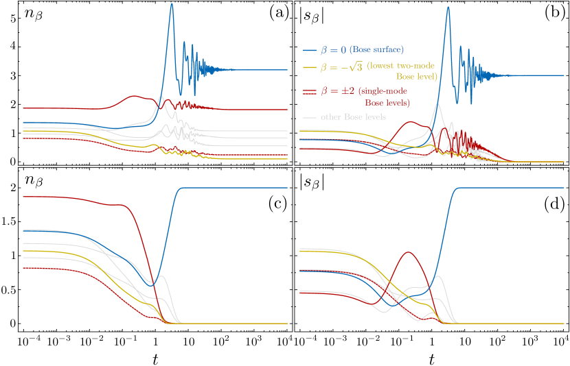
Figure 3: Numerical time-evolution of the Bose-level variables $n_{\beta}=\sum_{\bm{k}\in\mathrm{BL}_{\beta}}|\alpha_{\bm{k}}|^{2}$ and $s_{\beta}=\sum_{\bm{k}\in\mathrm{BL}_{\beta}}\alpha_{\bm{k}}\alpha_{-\bm{k}}$, which form a closed system ruled by Eqs. (8). As in Fig. 2, we consider a 1D situation with $L=12$, $\mu=0$, and $\varepsilon=3$, but the plots are qualitatively the same for any other choice of dimension, size, or parameters. We consider in (a) and (b) the $\kappa=0$ case, and in (c) and (d) the $\kappa=1$ case, starting from a random initial state. Again as in Fig. 2, we highlight the evolution of the Bose-surface (blue), the lowest nontrivial Bose level $\mathrm{BL}_{-\sqrt{3}}$ containing modes $k=\pm 5\pi/2$ (yellow), and the Bose levels $\mathrm{BL}_{\pm 2}$ with the largest and smallest values of the dispersion relation, which contain the single modes $k=0$ (solid red) and $\pi$ (dashed red), respectively. The simulations are consistent with the analytics discussed in the main text, showing that all population moves towards the Bose surface, except when $\kappa=0$, for which a population $\lim_{t\rightarrow\infty}n_{\beta\neq 0}(t)=C_{\beta}$ persists, associated with the oscillatory configurations discussed in Fig. 2 induced by the existence of the $C_{\beta}=\sqrt{n_{\beta}^{2}-|s_{\beta}|^{2}}$ constants of motion.

The story is completely different for the stationary solutions at other Bose levels. As we prove in Appendix E.3 and show in Fig. 2(d), for the stationary solution (10) at a given Bose-level even an infinitesimal fluctuation at Bose levels with smaller $|\beta|$ will precipitate a cascade of the population towards the lowest-$|\beta|$ level, that is, towards the Bose surface. The cascade proceeds until just the small population $n_{\beta}=\delta C_{\beta}$ related to the level constant induced by the initial fluctuations, $\delta C_{\beta}^{2}=n_{\beta}^{2}(0)-|s_{\beta}(0)|^{2}$, remains in Bose levels other than the Bose surface. Hence, these stationary solutions are very unstable, and moreover reinforce the idea that the Bose-surface solution is (marginally) stable.

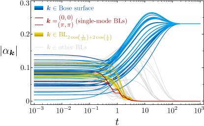
Figure 4: Numerical simulation of the time evolution of $\alpha_{\bm{k}}(t)$ from the Gross-Pitaevskii equations (5) in 2D ($d=2$) for a lattice of size $L\times L=20\times 20$. We have included a weak driving term $\sum_{\bm{k}\in\mathrm{BS}}\mathrm{i}F(\hat{b}_{\bm{k}}^{\dagger}-\hat{b}_{\bm{k}})$ with $F=0.01$, where $\hat{b}_{\bm{k}}=\sum_{\bm{j}}e^{\mathrm{i}\bm{k}\cdot\bm{j}}\hat{a}_{\bm{j}}/L$ are the annihilation operators for the Fourier modes. The rest of parameters are $\kappa=1$, $\mu=0$, and $\varepsilon=3$, leading to a Bose surface with 38 modes (blue). We also show the single-mode Bose levels at the edge and center of the Brillouin zone (red), the 8 modes of the Bose level with $\beta=2\cos(1/10)+2\cos(1/2)$ (yellow), and the modes of 10 other random Bose surfaces (grey). Starting from random initial conditions, we find that a weak driving is enough to bias a final state with all modes of the Bose surface equally populated, while all other Bose levels remain unpopulated. Moreover, we have found that driving differently each $\pm\bm{k}$ pair, one can distribute the total density in any desired way within the Bose surface modes. Hence, this simulations show that a weak driving can be used to “write” any unconventional superfluid state with all population distributed at will along a closed manifold in Fourier space.

In summary, in the absence of linear local dissipation ($\kappa=0$), the asymptotic configuration of the system corresponds to one in which the population is concentrated at the Bose surface in the form of a stationary solution with $n_{0}=\sqrt{C_{0}^{2}+\varepsilon^{2}}$, except for some leftover population $n_{\beta\neq 0}=C_{\beta}=\sqrt{n_{\beta}^{2}(0)-|s_{\beta}(0)|^{2}}$ at other Bose levels, for which the amplitudes $\alpha_{\bm{k}\in\mathrm{BL}_{\beta}}$ oscillate in time at frequency $\beta$. The specific way in which the population is distributed over the $\bm{k}$ modes of a given Bose level is only constrained by $s_{0}=-\mathrm{i}\varepsilon$ at the Bose surface and $\alpha_{\bm{k}}\alpha_{-\bm{k}}=0$ at other Bose levels.

Figure 5: Sketch of our implementation proposal with superconducting circuits. The main system consists of an array of LC oscillators (yellow) with distinct frequencies $\omega_{j}$, which exchange excitations at rates that can be tuned through local magnetic fluxes, represented by $B_{j}(t)$ in the figure. The array couples through a Josephson junction (white) to a coherent microwave generator (red) and an additional lossy LC circuit (blue) driven by a resonant generator, which induces a coherent state of amplitude $\alpha_{\mathrm{p}}e^{-\mathrm{i}\Omega_{\mathrm{p}}t}$ in the circuit. When the decay rate $\kappa_{\mathrm{p}}$ of the pump circuit is the dominant rate, and the microwave tones $\nu_{m}$, circuit frequencies, and magnetic fluxes are chosen appropriately (see the main text), the array evolves according to our model’s master equation.

V Effect of local linear dissipation

With the previous results in mind, it is easy to understand what happens when introducing linear local dissipation $\kappa\neq 0$. As we argue next, the main effect of $\kappa$ is making the stationary configurations at the Bose surface even more robust, that is, to remove any trace of population in other Bose levels. But, remarkably, even under these conditions the way in which the population is distributed along the Bose surface remains arbitrary, and it can be biased with a judicious initial condition or with a weak drive, as we show below. In particular, this allows for configurations in which all the $\bm{k}$ modes of the closed manifold are populated. This is an exotic state of outmost importance in condensed-matter physics for its connection with high-$T_{\text{c}}$ superconductivity (Jiang et al., 2019), frustrated magnetism (Sedrakyan et al., 2015), and interacting problems with spin-orbit coupling (Wu et al., 2011; Gopalakrishnan et al., 2011).

Let us start by noting that, using Eqs. (8), the level constants are easily shown to satisfy

$$\dot{C}_{\beta}=-2\kappa C_{\beta}\Longrightarrow\lim_{t\rightarrow\infty}C_{\beta}(t)=0\,\forall\beta.$$ (15)

The level constants are not conserved anymore; instead, they are forced to vanish asymptotically by the local dissipation. This is accompanied by two effects. First, now that the level constants are zero, there is no reason for any population to remain at Bose levels other than the Bose surface. Indeed, our exhaustive simulations show that all population flows towards the Bose surface asymptotically, irrespective of the initial state, as shown in Fig. 3(b). In particular, the system reaches a fixed point of the Bose-level equations (8) with

$$\left\{\begin{array}[]{cc}n_{\beta}=s_{\beta}=0,&\text{if }\mathrm{BL}_{\beta}\neq\mathrm{BS}\\ n_{\beta}=\varepsilon-\kappa=\mathrm{i}s_{\beta},&\text{if }\mathrm{BL}_{\beta}=\mathrm{BS}\end{array}\right..$$ (16)

Note that now it is necessary that $\varepsilon>\kappa$ for this solution to exist, also required in order to destabilize the trivial solution $\alpha_{\bm{k}}=0\,\forall\bm{k}$, whose fluctuations will only grow once driving provides enough energy to balance dissipation, as explicitly shown in Appendix E.1. The flow of the population towards the Bose surface is further supported by the stability analysis of the stationary solutions at Bose levels different than the Bose surface, which we detail in Appendices B and E.3, and proves that these solutions become more unstable the larger $\kappa$ is. In contrast, the stationary solution at the Bose surface becomes more stable by increasing $\kappa$, as we show next.

The second effect connected to Eq. (15) that we want to discuss relates to the solution at the Bose surface. As we discussed in the previous section, a zero level constant implies that the configuration of the amplitudes $\alpha_{\bm{k}}=\rho_{\bm{k}}e^{\mathrm{i}\phi_{\bm{k}}}$ needs to be of the balanced type. Indeed, solving for the steady state of the GP equation (5) with $\alpha_{\bm{k}\notin\mathrm{BS}}=0$, one easily finds for $\bm{k}\in\mathrm{BS}$ that

$$\phi_{\bm{k}} +\phi_{-\bm{k}}=-\pi/2,$$ (17a)

$$\rho_{\bm{k}} =\rho_{-\bm{k}},\quad\sum_{\bm{k}\in\mathrm{BS}}\rho_{\bm{k}}^{2}=\varepsilon-\kappa.$$ (17b)

Any configuration satisfying these conditions is a robust one that can be biased by, e.g., tuning the initial condition or adding a weak linear driving with the desired spatial profile (see Fig. 4). We say that these configurations are robust because we show in Appendix E.2 that they are stable against any type of perturbation, except of course perturbations compatible with (17), which are not damped but also not amplified (making this solution marginally stable as expected). Hence, in this system we can write many interesting patterns, including periodic and quasi-periodic ones with an arbitrary number of opposite-Fourier modes $\pm\bm{k}$, as well as the exotic one presented in Fig. 4 where all the modes of the Bose surface are populated.

VI Implementation with superconducting circuit arrays

Superconducting circuits (Blais et al., 2021; Krantz et al., 2019; Gu et al., 2017) provide a very flexible platform where our ideas can be potentially explored. Arrays with up to $N=66$ quantum oscillators with tunable frequency, anharmonicity, and tunnelings have been already built (F. Arute et al., 2019; X. Mi et al., ; K. J. Satzinger et al., ; Wu et al., 2021; M. Gong et al., 2021; Q. Zhu et al., ; X. Zhang et al., ), and the number keeps growing strong in seek of the promised practical quantum computer. In addition, the pair driving and dissipation considered in our model has been implemented in single circuits by exploiting four-wave mixing at driven Josephson junctions (Leghtas et al., 2015; Touzard et al., 2018; Lescanne et al., 2020), also motivated by the quantum-computing goal of encoding noise-resilient qubits in the infinite-dimensional Hilbert space of a harmonic oscillator. Here we show that these experimental quantum computing breakthroughs can be combined and adapted to implement our pair-driven-dissipative many-body model, as schematically shown in Fig. 5.

We consider an array of LC circuits with different frequencies $\{\omega_{j}\}_{j=1,2,...,N}$ (take for notational simplicity a one-dimensional system). These LC circuits are linearly coupled through an intermediary circuit that is sensitive to an external magnetic field. This allows for real-time control of the hopping rates (F. Arute et al., 2019), which we set to $J\exp[-\mathrm{i}(\omega_{j}-\omega_{j-1})t]$ between circuits $j-1$ and $j$. Through a Josephson junction driven by a microwave generator that feeds coherent tones at frequencies $\{\nu_{m}\}_{m=1,2,...,N}$, all circuits of the array are connected to an additional driven and lossy LC circuit, dubbed ‘pump’ resonator, with frequency $\Omega_{\mathrm{p}}$. The four-wave-mixing frequency-conversion process $\Omega_{\mathrm{p}}+\nu_{n}\rightleftharpoons\omega_{j}+\omega_{l}$ occurs at the junction (Leghtas et al., 2015; Touzard et al., 2018; Lescanne et al., 2020), so that the evolution of the system’s state $\hat{\rho}_{0}$ is described by the master equation

$$\partial_{t}\hat{\rho}_{0}=-\mathrm{i}\left[\frac{\hat{H}_{0}(t)}{\hbar},\hat{\rho}_{0}\right]+\kappa_{\mathrm{p}}\mathcal{D}_{p}\left[\hat{\rho}_{0}\right],$$ (18)

with (periodic boundaries are assumed, so $j=0$ is understood to be equivalent to $j=N$)

$$\frac{\hat{H}_{0}}{\hbar}= \sum_{j=1}^{N}\left[\omega_{j}\hat{a}_{j}^{\dagger}\hat{a}_{j}-\left(Je^{-\mathrm{i}(\omega_{j}-\omega_{j-1})t}\hat{a}_{j-1}\hat{a}_{j}^{\dagger}+\mathrm{H.c.}\right)\right]$$

$$+ \sum_{mjl=1}^{N}g\left[e^{-\mathrm{i}\nu_{m}t}\left(\hat{p}+\alpha_{\mathrm{p}}e^{-\mathrm{i}\Omega_{\mathrm{p}}t}\right)\hat{a}_{j}^{\dagger}\hat{a}_{l}^{\dagger}+\mathrm{H.c.}\right],$$ (19)

where $\alpha_{\mathrm{p}}$ (assumed real and positive without loss of generalization) is the amplitude of the coherent state induced by the driving on the pump resonator, so that the operator $\hat{p}$ annihilates excitations around such coherent state. $g$ is the four-wave-mixing rate, controllable through the amplitude of the microwave tones, which we assume the same for all tones. In order to obtain the type of collective dissipation that we seek, the key idea consists in taking far-off resonant circuits with $|\omega_{j}-\omega_{l}|\gg g$ and tones $\nu_{j}=2\omega_{j}-\Omega_{\mathrm{p}}+2\mu$, where $\mu$ is a small frequency mismatch (detuning) that will play the role of the chemical potential in the model.

That these choices lead to the desired model is best seen by moving to a picture rotating at frequency $\Omega_{\mathrm{p}}$ for the pump and $\omega_{j}+\mu$ for circuit $j$, effected by discounting the unitary evolution

$$\hat{U}(t)=\exp\biggl{[}-\mathrm{i}\Omega_{\mathrm{p}}t\hat{p}^{\dagger}\hat{p}-\mathrm{i}\sum_{j=1}^{N}(\omega_{j}+\mu)t\hat{a}_{j}^{\dagger}\hat{a}_{j}\biggr{]}.$$ (20)

The master equation of the transformed state $\hat{\rho}_{1}=\hat{U}^{\dagger}\hat{\rho}_{0}\hat{U}$ keeps the same form as (5), but with a modified Hamiltonian

$$\frac{\hat{H}_{1}}{\hbar} =-\sum_{j=1}^{N}\left[\mu\hat{a}_{j}^{\dagger}\hat{a}_{j}+J\left(\hat{a}_{j-1}\hat{a}_{j}^{\dagger}+\mathrm{H.c.}\right)\right]$$ (21)

$$+\sum_{mjl=1}^{N}g\left[e^{\mathrm{i}\Omega_{mjl}t}\left(\hat{p}+\alpha_{\mathrm{p}}\right)\hat{a}_{j}^{\dagger}\hat{a}_{l}^{\dagger}+\mathrm{H.c.}\right],$$

with $\Omega_{mjl}=2\omega_{m}-\omega_{j}-\omega_{l}$. It is clear that $\Omega_{jjj}=0\,\forall j$, and we assume that the frequencies are chosen in such a way that $|\Omega_{mjl}|\gg g\alpha_{\mathrm{p}}$ for any other value of the indices $(m,j,l)$. Then, the rotating-wave approximation allows us to neglect all time-dependent terms in the Hamiltonian, which then takes the form

$$\frac{\hat{H}_{1}}{\hbar}=\frac{\hat{H}}{\hbar}+g\biggl{(}\hat{p}\sum_{j=1}^{N}\hat{a}_{j}^{\dagger 2}+\mathrm{H.c.}\biggr{)},$$ (22)

where $\hat{H}$ is the Hamiltonian (2a) of our model (with $\varepsilon=2g\alpha_{\mathrm{p}}$). We see that the pump mode couples to the collective jump operator of our model, $\sum_{j=1}^{N}\hat{a}_{j}^{\dagger 2}$. Hence, adiabatically eliminating the pump under the assumption that its damping rate $\kappa_{\mathrm{p}}$ is much larger than any other rate ($\mu$, $J$, $\varepsilon$, $g$, and $\kappa$), it is straightforward to show (Benito et al., 2016) that the reduced state $\hat{\rho}=\mathrm{tr}_{\mathrm{p}}\{\hat{\rho}_{1}\}$ of the array evolves according to the master equation (1) of our model with $\gamma/N=2g^{2}/\kappa_{\mathrm{p}}$.

As for $\kappa$, we note that local decay is always present to a certain extent in the circuits, while incoherent pumping can be implemented in several known ways (Navarrete-Benlloch et al., 2014; Marthaler et al., 2011; Grajcar et al., 2008; Astafiev et al., 2007).

VII Conclusions

In this work we have shown that including quantum-optical processes such as pair driving and dissipation on many-body models characteristic of condensed-matter physics, one gets access to physics beyond the paradigm accessible to these disciplines on their own. As a means of example, we have considered a bosonic array in which all bosonic nodes are pair-driven through the same source, leading to collective pair-dissipation rather than local one. The resulting model, including experimentally unavoidable local linear dissipation, has been shown to lead to incredibly rich and controllable spatiotemporal phenomena within the superfluid phase. In particular, we have proven that the condensates are stabilized into an exotic configuration where only the modes of a closed manifold in Fourier space are populated, with a distribution of the population along the manifold that we can bias through the initial conditions or through a weak external drive. This allows to stabilize, for example, a condensate populating a finite number of $\pm\bm{k}$ pairs of Fourier wave vectors that can be controlled by judiciously choosing a target Bose surface (experimentally tunable via the detuning $\mu$), leading to periodic and quasi-periodic patterns with a tunable spatial (quasi-)period and orientation. We have also shown explicitly how to stabilize a pattern where all the modes of the closed manifold are equally populated, which is a state conjectured to play an important role in some open condensed-matter problems such as high-$T_{\text{c}}$ superconductivity. In addition, by balancing any residual local linear decay through an incoherent pumping mechanism, we have shown that new constants of motion emerge, that force the condensate to get nontrivial temporal order in the form of robust oscillations at different frequency for each Bose level. This behavior generalizes the one found in superfluid time-crystals, where particle-number conservation leads to robust oscillations of the macroscopic wave function at a frequency set by the chemical potential. Finally, we have put forward a generic way in which our model can be implemented by exploiting four-wave mixing in superconducting circuits. This opens the way to the experimental exploration of the condensates with nontrivial spatiotemporal order present in our unconventional driven-dissipative model.

Appendix A From the master equation
to the GP equations

In order to derive the GP equations (3) from the master equation, we start by noting that the equation of motion of the expectation value of any operator $\hat{A}$ can be found as

$$\partial_{t}\langle\hat{A}\rangle= \mathrm{tr}\{\hat{A}\partial_{t}\hat{\rho}\}=-\frac{\mathrm{i}}{\hbar}\langle[\hat{A},\hat{H}]\rangle$$ (23)

$$+\frac{\gamma}{2N}\left(\langle[\hat{J}^{\dagger},\hat{A}]\hat{J}\rangle+\langle\hat{J}^{\dagger}[\hat{A},\hat{J}]\rangle\right)$$

$$+\sum_{\bm{j}}\gamma_{0}\left(\langle[\hat{a}_{\bm{j}}^{\dagger},\hat{A}]\hat{a}_{\bm{j}}\rangle+\langle\hat{a}_{\bm{j}}^{\dagger}[\hat{A},\hat{a}_{\bm{j}}]\rangle\right)$$

$$+\sum_{\bm{j}}\Gamma\left(\langle[\hat{a}_{\bm{j}},\hat{A}]\hat{a}_{\bm{j}}^{\dagger}\rangle+\langle\hat{a}_{\bm{j}}[\hat{A},\hat{a}_{\bm{j}}^{\dagger}]\rangle\right),$$

where we have used the master equation (1) and defined $\hat{J}=\sum_{\bm{j}}\hat{a}_{\bm{j}}^{\dagger 2}$. Applied to the $\hat{a}_{\bm{j}}$ operators, we obtain

$$\partial_{t}\langle\hat{a}_{\bm{j}}\rangle= \mathrm{tr}\{\hat{A}\partial_{t}\hat{\rho}\}=(\mathrm{i}\mu-\gamma_{0}+\Gamma)\langle\hat{a}_{\bm{j}}\rangle-\mathrm{i}\varepsilon\langle\hat{a}_{\bm{j}}^{\dagger}\rangle$$ (24)

$$+\mathrm{i}J\sum_{\langle\bm{l}\rangle_{\bm{j}}}\langle\hat{a}_{\bm{l}}\rangle-\frac{\gamma}{N}\langle\hat{a}_{\bm{j}}^{\dagger}\sum_{\bm{l}}\hat{a}_{\bm{l}}^{\dagger 2}\rangle.$$

Assume now that the state of the system is coherent at all times, that is, $\bigotimes_{\bm{j}}|\psi_{\bm{j}}(t)\rangle$ with $\hat{a}_{\bm{j}}|\psi_{\bm{j}}\rangle=\psi_{\bm{j}}|\psi_{\bm{j}}\rangle$ and $\psi_{\bm{j}}\in\mathbb{C}$. Applying then $\langle\hat{a}_{\bm{l}_{1}}^{\dagger}...\hat{a}_{\bm{l}_{m}}^{\dagger}\hat{a}_{\bm{j}_{1}}...\hat{a}_{\bm{j}_{n}}\rangle=\psi_{\bm{l}_{1}}^{*}...\psi_{\bm{l}_{m}}^{*}\psi_{\bm{j}_{1}}...\psi_{\bm{j}_{n}}$ on (24), we obtain

$$\dot{\psi}_{\bm{j}}=\left(\mathrm{i}\mu-\kappa\right)\psi_{\bm{j}}-\Bigl{(}\mathrm{i}\varepsilon+\frac{\gamma}{N}\sum_{\bm{l}}\psi_{\bm{l}}^{2}\Bigr{)}\psi_{\bm{j}}^{*}+\mathrm{i}J\sum_{\left<\bm{l}\right>_{\bm{j}}}\psi_{\bm{j}}.$$ (25)

Finally, by defining normalized variables and parameters $\tilde{t}=Jt$, $\tilde{\psi}_{\bm{j}}=\sqrt{\gamma/JN}\psi_{\bm{j}}$, $\tilde{\mu}=\mu/J$, $\tilde{\varepsilon}=\varepsilon/J$, and $\tilde{\kappa}=\kappa/J$, we obtain the GP equation as presented in (3). Note however that we removed there the tildes to ease the notation, and also because the normalization is equivalent to setting $J$ and $\gamma/N$ to one in (25).

Appendix B Stationary solutions

Here we discuss in detail the stationary solutions present in the GP equations (5). We start by considering the stationary equations ($\dot{\alpha}_{\bm{k}}=0$) for an arbitrary pair $\pm\bm{k}$,

$$\left(\mathrm{i}\omega_{\bm{k}}-\kappa\right)\alpha_{\bm{k}} =\Bigl{(}\mathrm{\mathrm{i}}\varepsilon+\sum_{\bm{q}}\alpha_{\bm{q}}\alpha_{-\bm{q}}\Bigr{)}\alpha_{-\bm{k}}^{*},$$ (26a)

$$\left(\mathrm{i}\omega_{\bm{k}}+\kappa\right)\alpha_{-\bm{k}}^{*} =\Bigl{(}\mathrm{\mathrm{i}}\varepsilon-\sum_{\bm{q}}\alpha_{\bm{q}}^{*}\alpha_{-\bm{q}}^{*}\Bigr{)}\alpha_{\bm{k}}.$$ (26b)

Taking their product, we obtain

$$\Bigl{|}\mathrm{i}\varepsilon+\sum_{\bm{q}}\alpha_{\bm{q}}\alpha_{-\bm{q}}\Bigr{|}^{2}=\omega_{\bm{k}}^{2}+\kappa^{2}-\varepsilon^{2}.$$ (27)

Now, the left-hand-side of this expression is independent of $\bm{k}$, while the right-hand-side depends on it through $\omega_{\bm{k}}^{2}$. Therefore, the excitation of two modes with different absolute value of the dispersion $|\omega_{\bm{k}}|$ is incompatible, and thus, stationary solutions can only populate the modes of Bose levels with opposite dispersion. Note that the Bose surface, being defined by $\omega_{\bm{k}}=0$, admits stationary solutions where it is populated by itself. This stationary solutions are easily found directly from the GP equation as explained in the main text.

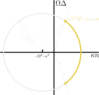
Figure 6: The stationary configurations outside of the Bose surface can populate simultaneously two Bose levels $\omega_{\bm{k}}=\pm\Omega$ with opposite dispersion. $n$ is the total population and $\Delta$ the difference of population between the levels. These stationary configurations lie on a segment (thick yellow curve) of the circle shown in the figure in the $(\kappa n,\Omega\Delta)$ space.

We consider then a stationary solution that populates only two Bose levels defined by $\omega_{\bm{k}}=\pm\Omega$, with $\Omega>0$, which we denote by $\mathrm{BL}_{\pm}$ (the analysis will naturally accommodate also situations in which one of the $\mathrm{BL}_{\pm}$ do not exist, equivalent to leaving it unpopulated in the upcoming analysis). In terms of the Bose-level variables (7), we then have $\sum_{\bm{q}}\alpha_{\bm{q}}\alpha_{-\bm{q}}=s_{+}+s_{-}$. On the other hand, multiplying Eq. (26a) by $\alpha_{-\bm{k}}$ and summing over all the modes of $\mathrm{BL}_{\pm}$, we obtain the equations

$$(\mathrm{i}\Omega-\kappa)s_{+} =(\mathrm{i}\varepsilon+s_{+}+s_{-})n_{+},$$ (28a)

$$-(\mathrm{i}\Omega+\kappa)s_{-} =(\mathrm{i}\varepsilon+s_{+}+s_{-})n_{-}.$$ (28b)

Similarly, multiplying Eq. (26a) by $\alpha_{\bm{k}}^{*}$ and summing over all modes at $\mathrm{BL}_{\pm}$, we get

$$(\mathrm{i}\Omega-\kappa)n_{+} =(\mathrm{i}\varepsilon+s_{+}+s_{-})s_{+}^{*},$$ (29a)

$$-(\mathrm{i}\Omega+\kappa)n_{-} =(\mathrm{i}\varepsilon+s_{+}+s_{-})s_{-}^{*}.$$ (29b)

The first thing to note is that $|s_{\pm}|=n_{\pm}$ as follows from (28a)/(29a) and (28b)/(29b). As shown in Appendix D and mentioned in the text, this implies that the configurations $\alpha_{\bm{k}}$ at both Bose levels are of the balanced type, which we will also show here explicitly shortly. Let us now define the total population $n=n_{+}+n_{-}$ and the difference of populations $\Delta=n_{+}-n_{-}$. Operating on the previous equations as $(\mathrm{i}\Omega-\kappa)($28b$)-(\mathrm{i}\Omega+\kappa)($28a$)$, it is easy to get

$$\mathrm{i}\varepsilon+s_{+}+s_{-}=\frac{\varepsilon(\Omega^{2}+\kappa^{2})}{\Omega\Delta-\mathrm{i}(\Omega^{2}+\kappa^{2}+\kappa n)}.$$ (30)

But, at the same time, from the balance condition $|s_{\pm}|=n_{\pm}$ and the absolute value of either (28) or (29), we know that $|\mathrm{i}\varepsilon+s_{+}+s_{-}|^{2}=\Omega^{2}+\kappa^{2}$, so equating this to the absolute value of (30) we obtain

$$\Omega^{2}\Delta^{2}+(\Omega^{2}+\kappa^{2}+\kappa n)^{2}=\varepsilon^{2}(\Omega^{2}+\kappa^{2}).$$ (31)

We then see that, on the $(\kappa n,\Omega\Delta)$ space, the accessible configurations lie on a circle of radius $\varepsilon\sqrt{\Omega^{2}+\kappa^{2}}$, centered at point $-(\Omega^{2}+\kappa^{2},0)$, see Fig. 6. Hence, if we want at least part of the circle to lie on the physical space $n>0$, the condition $\varepsilon>\sqrt{\Omega^{2}+\kappa^{2}}$ must be satisfied, meaning that the radius is larger than the distance between the center and the origin of the reference axes. In addition, the $|\Delta|\leq n$ constraint restricts further the physical region of the circle (31), so that only its segment between points $(\sqrt{\varepsilon^{2}-\Omega^{2}}-\kappa)\times(\kappa,\pm\Omega)$ is available. Note that these points correspond to configurations where only one Bose level is populated, $\mathrm{BL}_{\pm}$, respectively. We summarize all these features in Fig. 6. Note also that when $\kappa=0$, the ellipse degenerates into the lines $|\Delta|=\sqrt{\varepsilon^{2}-\Omega^{2}}$ with $n$ bounded only $n>|\Delta|$, which is the case we discussed explicitly in the main text, see Eq. (10).

Now that we know that $\mathrm{i}\varepsilon+s_{+}+s_{-}=\sqrt{\Omega^{2}+\kappa^{2}}e^{\mathrm{i}\theta}$, with $\theta=\arg\{\Omega\Delta+\mathrm{i}(\Omega^{2}+\kappa^{2}+\kappa n)\}$, we can insert it into Eq. (26a), which then tells us that the configuration of the amplitudes at the Bose levels must satisfy

$$\alpha_{\bm{-k}\in\mathrm{BL}_{\pm}}=-\mathrm{i}e^{\mathrm{i}\varphi_{\pm}}\alpha_{\bm{k}}^{*},$$ (32)

with $\varphi_{\pm}=\arg\left\{(\pm\Omega+\mathrm{i}\kappa)[\Omega\Delta n+\mathrm{i}(\Omega^{2}+\kappa^{2}+\kappa n)]\right\}$. Setting $\kappa=0$ we recover the phases $\varphi_{\pm}$ presented in the main text, Eq. (10), but now we see that even when for $\kappa\neq 0$, the configurations must be of the balanced type. Any configuration that satisfies Eqs. (31) and (32) is allowed as a stationary solution of the system, but we show in Appendix E.3 that they are unstable configurations.

Appendix C Oscillatory solutions

Our numerics suggest that the oscillatory solutions found for $\kappa=0$ are of the harmonic form $\alpha_{\bm{k}}(t)=\bar{\alpha}_{\bm{k}}e^{\mathrm{i}\nu_{\bm{k}}t}$, with $\bar{\alpha}_{\bm{k}}$ independent of time. Inserting this ansatz into the GP equation (5), we obtain

$$(\omega_{\bm{k}}\negthinspace-\negthinspace\nu_{\bm{k}})\bar{\alpha}_{\bm{k}}e^{\mathrm{i}(\nu_{\bm{k}}+\nu_{-\bm{k}})t}\negthinspace=\negthinspace\Bigl{(}\varepsilon-\mathrm{\mathrm{i}}\negthinspace\sum_{\forall\bm{q}}\bar{\alpha}_{\bm{q}}\bar{\alpha}_{-\bm{q}}e^{\mathrm{i}(\nu_{\bm{q}}+\nu_{-\bm{q}})t}\Bigr{)}\bar{\alpha}_{-\bm{k}}^{*}.$$ (33)

In addition, from our exhaustive numerical simulations, we know that the Bose-level equations always reach asymptotically the fixed point (14), which means that

$$\sum_{\forall\bm{k}}\alpha_{\bm{k}}\alpha_{-\bm{k}}=\sum_{\beta}s_{\beta}=-\mathrm{i}\varepsilon.$$ (34)

This is only compatible with the oscillatory solution if $\nu_{-\bm{k}}=-\nu_{\bm{k}}$. The right-hand-side of Eq. (33) then vanishes, while particularizing the left-hand-side to a given $\pm\bm{k}$ pair we obtain

$$(\beta-\nu_{\bm{k}})\bar{\alpha}_{\bm{k}}=0=(\beta+\nu_{\bm{k}})\bar{\alpha}_{-\bm{k}}.$$ (35)

For a generic Bose level different than the Bose surface, these conditions can be satisfied only if one of the amplitudes $\bar{\alpha}_{\pm\bm{k}}$ vanishes, and the other oscillates with $\nu_{\pm\bm{k}}=\beta$. For the Bose surface $\beta=0$, so that these conditions imply $\nu_{\bm{k}}=0$, meaning that the asymptotic amplitudes $\alpha_{\bm{k}}$ are stationary and only constrained by (14).

Appendix D Interpretation of the level constants

The level constants (11) can be written as

$$C_{\beta}^{2}=\sum_{\bm{k}\bm{k}^{\prime}\in\mathrm{BL}_{\beta}}\left(|\alpha_{\bm{k}}|^{2}|\alpha_{\bm{k}^{\prime}}|^{2}-\alpha_{\bm{k}}\alpha_{-\bm{k}}\alpha_{\bm{k}^{\prime}}^{*}\alpha_{-\bm{k}^{\prime}}^{*}\right).$$ (36)

In the following we show that this constants are positive or zero, vanishing only when the configuration $\alpha_{\bm{k}}=\rho_{\bm{k}}e^{\mathrm{i}\phi_{\bm{k}}}$ of the system is of the balanced type, that is, $\rho_{\bm{k}}=\rho_{-\bm{k}}$ with $\phi_{\bm{k}}+\phi_{-\bm{k}}$ fixed to a value that depends only on the Bose level where $\bm{k}$ lies in. In order to see this, we consider two types of terms in the sum (36), and bound them separately. First we consider the terms with $\bm{k}^{\prime}=\pm\bm{k}$, and write explicitly the $\pm\bm{k}$ contributions to the sum,

$$A_{\bm{k}}\equiv |\alpha_{\bm{k}}|^{4}+|\alpha_{-\bm{k}}|^{4}+2|\alpha_{\bm{k}}|^{2}|\alpha_{-\bm{k}}|^{2}-4\alpha_{\bm{k}}\alpha_{-\bm{k}}\alpha_{\bm{k}}^{*}\alpha_{-\bm{k}}^{*}.$$ (37)

Next, we consider the terms with $\bm{k}\neq\bm{k}^{\prime}$, and again write down explicitly the $\pm\bm{k}$ and $\pm\bm{k}^{\prime}$ contributions,

$$B_{\bm{k}\bm{k}^{\prime}}\equiv (|\alpha_{\bm{k}}|^{2}+|\alpha_{-\bm{k}}|^{2})(|\alpha_{\bm{k}^{\prime}}|^{2}+|\alpha_{-\bm{k}^{\prime}}|^{2})$$ (38)

$$-2\alpha_{\bm{k}}\alpha_{-\bm{k}}\alpha_{\bm{k}^{\prime}}^{*}\alpha_{-\bm{k}^{\prime}}^{*}-2\alpha_{\bm{k}^{\prime}}\alpha_{-\bm{k}^{\prime}}\alpha_{\bm{k}}^{*}\alpha_{-\bm{k}}^{*}.$$

In terms of these objects, the level constants can be written as

$$C_{\beta}^{2}=\frac{1}{4}\sum_{\bm{k}\in\mathrm{BL}_{\beta}}\Bigl{(}2A_{\bm{k}}+\underset{\bm{k}^{\prime}\neq\pm\bm{k}}{\sum_{\bm{k}^{\prime}\in\mathrm{BL}_{\beta}}}B_{\bm{k}\bm{k}^{\prime}}\Bigr{)}.$$ (39)

Now we proceed to bound the first type of terms, which is quite trivial since

$$A_{\bm{k}}=\rho_{\bm{k}}^{4}+\rho_{-\bm{k}}^{4}-2\rho_{\bm{k}}^{2}\rho_{-\bm{k}}^{2}=(\rho_{\bm{k}}^{2}-\rho_{-\bm{k}}^{2})^{2}\geq 0,$$ (40)

with the equality achieved only if $\rho_{\bm{k}}=\rho_{-\bm{k}}$. The second type of terms requires a bit more work

$$B_{\bm{k}\bm{k}^{\prime}}= \rho_{\bm{k}}^{2}\rho_{\bm{k}^{\prime}}^{2}+\rho_{\bm{k}}^{2}\rho_{-\bm{k}^{\prime}}^{2}+\rho_{-\bm{k}}^{2}\rho_{\bm{k}^{\prime}}^{2}+\rho_{-\bm{k}}^{2}\rho_{-\bm{k}^{\prime}}^{2}$$ (41)

$$-2\rho_{\bm{k}}\rho_{-\bm{k}}\rho_{\bm{k}^{\prime}}\rho_{-\bm{k}^{\prime}}\cos(\phi_{\bm{k}}+\phi_{-\bm{k}}-\phi_{\bm{k}^{\prime}}-\phi_{-\bm{k}^{\prime}})$$

$$\geq (\rho_{\bm{k}}\rho_{\bm{k}^{\prime}}-\rho_{-\bm{k}}\rho_{-\bm{k}^{\prime}})^{2}+(\rho_{\bm{k}}\rho_{-\bm{k}^{\prime}}-\rho_{-\bm{k}}\rho_{\bm{k}^{\prime}})^{2}\geq 0,$$

where in the last line we have upper-bounded the cosine by 1, and combined the resulting terms into a sum of squares. Note that the final equality is achieved in this case only when the amplitudes satisfy the balanced conditions $\phi_{\bm{k}}+\phi_{-\bm{k}}=\phi_{\bm{k}^{\prime}}+\phi_{-\bm{k}^{\prime}}$, $\rho_{\bm{k}}=\rho_{-\bm{k}}$, and $\rho_{\bm{k}^{\prime}}=\rho_{-\bm{k}^{\prime}}$. This concludes the proof and shows that $C_{\beta}=0$ if and only if the configuration of amplitudes $\alpha_{\bm{k}\in\mathrm{BL}_{\beta}}$ is balanced, otherwise $C_{\beta}>0$.

As a small detail, note that we have considered a nontrivial Bose level with more than 4 distinct wave vectors. In the one-dimensional case $d=1$ (where there are at most two wave vectors at a given Bose level) it’s trivial to see that the the level constants vanish when the amplitudes $\alpha_{\pm k}$ have have equal magnitude, as we saw in the text, while for single-wave-vector levels with $\bm{k}=(0,...,0)$ or $-(\pi,...,\pi)$ the level constants are zero by construction.

Appendix E Stability analysis

E.1 Trivial solution

The trivial stationary solution reads $\alpha_{\bm{k}}=0\,\forall\bm{k}$. Considering fluctuations $d_{\bm{k}}$ around it, and expanding the GP equations (5) to first order in these, we obtain the linear set

$$\left(\begin{array}[]{c}\dot{d}_{\bm{k}}\\ \dot{d}_{-\bm{k}}^{*}\end{array}\right)=\left(\begin{array}[]{cc}\mathrm{i}\omega_{\bm{k}}-\kappa&-\mathrm{\mathrm{i}}\varepsilon\\ \mathrm{\mathrm{i}}\varepsilon&-\mathrm{i}\omega_{\bm{k}}-\kappa\end{array}\right)\left(\begin{array}[]{c}d_{\bm{k}}\\ d_{-\bm{k}}^{*}\end{array}\right).$$ (42)

The eigenvalues of the linear stability matrix read in this case as $-\kappa\pm\sqrt{\varepsilon^{2}-\omega_{\bm{k}}^{2}}$. We then see that the fluctuations associated to modes $\pm\bm{k}$ will grow only if the driving satisfies $\varepsilon>\sqrt{\kappa^{2}+\omega_{\bm{k}}^{2}}$. Since the Bose-surface modes have $\omega_{\bm{k}\in\mathrm{BS}}=0$, these are the modes whose fluctuations get the largest divergence rate, as long as $\varepsilon>\kappa$. In the $\kappa=0$ case, this happens for any infinitesimal value of $\varepsilon$.

E.2 $\mathrm{BS}$ solution

Consider now the stationary solution (9) with only the Bose-surface modes excited, that is, $\lim_{t\rightarrow\infty}\alpha_{\bm{k}}(t)=\bar{\alpha}_{\bm{k}}$, with $\bar{\alpha}_{\bm{k}\notin\mathrm{BS}}=0$ and $\bar{\alpha}_{\bm{k}\in\mathrm{BS}}$ constrained by the condition $\sum_{\bm{k}\in\mathrm{BS}}\bar{\alpha}_{\bm{k}}\bar{\alpha}_{-\bm{k}}=\mathrm{i}(\kappa-\varepsilon)$. Considering now fluctuations around this solution, that is, $\alpha_{\bm{k}}(t)=\bar{\alpha}_{\bm{k}}+d_{\bm{k}}(t)$, the GP equations (5) are written to first order in the fluctuations as

$$\dot{d}_{\bm{k}}=(\mathrm{i}\omega_{\bm{k}}-\kappa)d_{\bm{k}}-\mathrm{i}\kappa d_{-\bm{k}}^{*}-2\bar{\alpha}_{-\bm{k}}^{*}\sum_{\mathbf{q}\in\mathrm{BS}}\bar{\alpha}_{-\bm{q}}d_{\bm{q}}.$$ (43)

Let us remark that this equation is valid both for $\kappa$ equal or different than zero.

Consider first fluctuations off the Bose surface, that is, $\bm{k}\notin\mathrm{BS}$. The equations can be recasted as the linear system

$$\left(\begin{array}[]{c}\dot{d}_{\bm{k}}\\ \dot{d}_{-\bm{k}}^{*}\end{array}\right)=\left(\begin{array}[]{cc}\mathrm{i}\omega_{\bm{k}}-\kappa&-\mathrm{\mathrm{i}}\kappa\\ \mathrm{\mathrm{i}}\kappa&-\mathrm{i}\omega_{\bm{k}}-\kappa\end{array}\right)\left(\begin{array}[]{c}d_{\bm{k}}\\ d_{-\bm{k}}^{*}\end{array}\right),$$ (44)

leading to a linear stability matrix with eigenvalues $-\kappa\pm\sqrt{\kappa^{2}-\omega_{\bm{k}}^{2}}$. For $\kappa\neq 0$, the real part of these eigenvalues is always negative, and hence, fluctuations damp back to the stationary solution. In contrast, when $\kappa=0$ the eigenvalues become $\pm\mathrm{i}\omega_{\bm{k}}$, showing that the fluctuations $d_{\pm\bm{k}}$ remain oscillating at frequency $\omega_{\bm{k}}$ around the stationary solution, without damping or amplification.

The situation is more subtle when the fluctuations lie on the Bose surface, that is, $\bm{k}\in\mathrm{BS}$ so that $\omega_{\bm{k}}=0$. In this case it is best to consider the evolution equation of the total fluctuation population, which from (43) is easily found to be

$$\frac{d}{dt}\left(\sum_{\bm{k}\in\mathrm{BS}}|d_{\bm{k}}|^{2}\right)= -4\left|\sum_{\bm{k}\in\mathrm{BS}}\bar{\alpha}_{-\bm{k}}d_{\bm{k}}\right|^{2}$$ (45)

$$-2\kappa\sum_{\bm{k}\in\mathrm{BS}}\left(|d_{\bm{k}}|^{2}+\mathrm{Im}\{d_{\bm{k}}d_{-\bm{k}}\}\right).$$

The first term is obviously negative or zero. It’s easy to show that the second term is also negative or zero, since expressing the fluctuations in magnitude and phase as $d_{\bm{k}}=r_{\bm{k}}e^{\mathrm{i}\varphi_{\bm{k}}}$, we have

$$\sum_{\bm{k}\in\mathrm{BS}}\mathrm{Im}\{d_{\bm{k}}d_{-\bm{k}}\} =\sum_{\bm{k}\in\mathrm{BS}}r_{\bm{k}}r_{-\bm{k}}\sin(\varphi_{\bm{k}}+\varphi_{-\bm{k}})$$ (46)

$$\geq-\sum_{\bm{k}\in\mathrm{BS}}r_{\bm{k}}r_{-\bm{k}} \geq-\sum_{\bm{k}\in\mathrm{BS}}r_{\bm{k}}^{2}=-\sum_{\bm{k}\in\mathrm{BS}}|d_{\bm{k}}|^{2}.$$

Note that the equality is obtained when $r_{\bm{k}}=r_{-\bm{k}}$ and $\varphi_{\bm{k}}+\varphi_{-\bm{k}}=-\pi/2\,\forall\bm{k}$, which means that the fluctuations perturb the solution in a way compatible with keeping it balanced, which is a condition that stationary configurations must satisfy when $\kappa\neq 0$, see Eq. (17). Note also that when $\kappa=0$ this contribution is directly zero.

This shows that the fate of the fluctuations is either to damp back to the stationary solution, or remain where they are when all terms in the right-hand-side of Eq. (45) are equal to zero. We have seen that, at least for the second term, this happens when the fluctuations connect with a new valid stationary solution. In order to prove that this is the same for the first term, just note that to first order in the fluctuations

$$\sum_{\bm{k}\in\mathrm{BS}}\alpha_{\bm{k}}\alpha_{\bm{-k}}\approx\sum_{\bm{k}\in\mathrm{BS}}\bar{\alpha}_{\bm{k}}\bar{\alpha}_{\bm{-k}}+2\sum_{\bm{k}\in\mathrm{BS}}\bar{\alpha}_{-\bm{k}}d_{\bm{k}},$$ (47)

so that fluctuations satisfying $\sum_{\bm{k}\in\mathrm{BS}}\bar{\alpha}_{-\bm{k}}d_{\bm{k}}=0$ lead to configurations that keep the constraint (9) invariant.

E.3 $\mathrm{BL}_{\beta}\neq\mathrm{BS}$ solutions

The easiest way to show that the stationary solutions at Bose levels other than the Bose surface are unstable is by performing the linear stability analysis from the Bose-level equations (8). We studied the form of these stationary solutions in Appendix B, in particular showing that they satisfy $\mathrm{i}\varepsilon+\sum_{\beta}s_{\beta}=\sqrt{\Omega^{2}+\kappa^{2}}e^{\mathrm{i}\theta}$, where $\omega_{\bm{k}}=\pm\Omega$ defines the two Bose levels that are populated. Remarkably, this is all we need to know in order to understand the stability of these stationary configurations (and we don’t even need the specific dependence of $\theta$ on the system parameters). For this, we consider the Bose-level equations (8) for an unpopulated Bose level $\beta\neq\pm\Omega$, and linearize them with respect to fluctuations $\delta s_{\beta}(t)$ and $\delta n_{\beta}(t)$ around the stationary solution $s_{\beta}=0=n_{\beta}$. Defining the vector $\delta\bm{r}_{\beta}=(\delta s_{\beta},\delta s_{\beta}^{*},\delta n_{\beta})^{T}$, we obtain a linear system $\delta\dot{\bm{r}}_{\beta}=\mathcal{L}_{\beta}\delta\bm{r}_{\beta}$, with a linear stability matrix (we further define $\sigma=\sqrt{\Omega^{2}+\kappa^{2}}$)

$$\mathcal{L}_{\beta}=-2\left(\begin{array}[]{ccc}\kappa-\mathrm{i}\beta&0&\sigma e^{\mathrm{i}\theta}\\ 0&\kappa+\mathrm{i}\beta&\sigma e^{-\mathrm{i}\theta}\\ \sigma e^{-\mathrm{i}\theta}/2&\sigma e^{\mathrm{i}\theta}/2&\kappa\end{array}\right),$$ (48)

which has eigenvalues $-2\kappa$ and $-2\Bigl{(}\kappa\pm\sqrt{\kappa^{2}+\Omega^{2}-\beta^{2}}\Bigr{)}$. The fluctuations $\delta\bm{r}_{\beta}$ of Bose levels with $|\beta|<|\Omega|$ will then grow away from the stationary solution, since one of the eigenvalues is positive for them. This shows that the stationary solutions at any Bose level other than the Bose surface (which has the minimum $\beta=0$) are unstable.

References

- Cirac and Zoller (2012) J. I. Cirac and P. Zoller, Nat. Phys. 8, 264 (2012).
- Bloch et al. (2012) I. Bloch, J. Dalibard, and S. Nascimbène, Nat. Phys. 8, 267 (2012).
- Blatt and Roos (2012) R. Blatt and C. F. Roos, Nat. Phys. 8, 277 (2012).
- Aspuru-Guzik and Walther (2012) A. Aspuru-Guzik and P. Walther, Nat. Phys. 8, 285 (2012).
- Houck et al. (2012) A. A. Houck, H. E. Türeci, and J. Koch, Nat. Phys. 8, 292 (2012).
- Altman et al. (2021) E. Altman, K. R. Brown, G. Carleo, L. D. Carr, E. Demler, C. Chin, B. DeMarco, S. E. Economou, M. A. Eriksson, K.-M. C. Fu, M. Greiner, K. R. Hazzard, R. G. Hulet, A. J. Kollár, B. L. Lev, M. D. Lukin, R. Ma, X. Mi, S. Misra, C. Monroe, K. Murch, Z. Nazario, K.-K. Ni, A. C. Potter, P. Roushan, M. Saffman, M. Schleier-Smith, I. Siddiqi, R. Simmonds, M. Singh, I. Spielman, K. Temme, D. S. Weiss, J. Vučković, V. Vuletić, J. Ye, and M. Zwierlein, PRX Quantum 2, 017003 (2021).
- Bloch et al. (2008) I. Bloch, J. Dalibard, and W. Zwerger, Rev. Mod. Phys. 80, 885 (2008).
- Jaksch and Zoller (2005) D. Jaksch and P. Zoller, Annals of Physics 315, 52 (2005).
- Dutta et al. (2015) O. Dutta, M. Gajda, P. Hauke, M. Lewenstein, D.-S. Lühmann, B. A. Malomed, T. Sowiński, and J. Zakrzewski, Rep. Prog. Phys. 78, 066001 (2015).
- Schweizer et al. (2019) C. Schweizer, F. Grusdt, M. Berngruber, L. Barbiero, E. Demler, N. Goldman, I. Bloch, and M. Aidelsburger, Nature Phys. 15, 1168 (2019).
- Wintersperger et al. (2020) K. Wintersperger, M. Bukov, J. Näger, S. Lellouch, E. Demler, U. Schneider, I. Bloch, N. Goldman, and M. Aidelsburger, Phys. Rev. X 10, 011030 (2020).
- M. et al. (2021) B. H. M., S. Scherg, T. Kohlert, I. Bloch, and M. Aidelsburger, “Benchmarking a novel efficient numerical method for localized 1d fermi-hubbard systems on a quantum simulator,” (2021), arXiv:2105.06372 [quant-ph] .
- Koepsell et al. (2020) J. Koepsell, D. Bourgund, P. Sompet, S. Hirthe, A. Bohrdt, Y. Wang, F. Grusdt, E. Demler, G. Salomon, C. Gross, and I. Bloch, “Microscopic evolution of doped mott insulators from polaronic metal to fermi liquid,” (2020), arXiv:2009.04440 [cond-mat.quant-gas] .
- Sompet et al. (2021) P. Sompet, S. Hirthe, D. Bourgund, T. Chalopin, J. Bibo, J. Koepsell, P. Bojović, R. Verresen, F. Pollmann, G. Salomon, C. Gross, T. A. Hilker, and I. Bloch, “Realising the symmetry-protected haldane phase in fermi-hubbard ladders,” (2021), arXiv:2103.10421 [cond-mat.quant-gas] .
- Boll et al. (2016) M. Boll, T. A. Hilker, G. Salomon, A. Omran, J. Nespolo, L. Pollet, I. Bloch, and C. Gross, Science 353, 1257 (2016).
- Hilker et al. (2017) T. A. Hilker, G. Salomon, F. Grusdt, A. Omran, M. Boll, E. Demler, I. Bloch, and C. Gross, Science 357, 484 (2017).
- Hachmann et al. (2021) M. Hachmann, Y. Kiefer, J. Riebesehl, R. Eichberger, and A. Hemmerich, Phys. Rev. Lett. 127, 033201 (2021).
- Greif et al. (2015) D. Greif, G. Jotzu, M. Messer, R. Desbuquois, and T. Esslinger, Phys. Rev. Lett. 115, 260401 (2015).
- Zeiher et al. (2017) J. Zeiher, J.-y. Choi, A. Rubio-Abadal, T. Pohl, R. van Bijnen, I. Bloch, and C. Gross, Phys. Rev. X 7, 041063 (2017).
- Fukuhara et al. (2013a) T. Fukuhara, P. Schauß, M. Endres, S. Hild, M. Cheneau, I. Bloch, and C. Gross, Nature 502, 76 (2013a).
- Fukuhara et al. (2013b) T. Fukuhara, A. Kantian, M. Endres, M. Cheneau, P. Schauß, S. Hild, D. Bellem, U. Schollwöck, T. Giamarchi, C. Gross, I. Bloch, and S. Kuhr, Nature Phys. 9, 235 (2013b).
- Ebadi et al. (2021) S. Ebadi, T. T. Wang, H. Levine, A. Keesling, G. Semeghini, A. Omran, D. Bluvstein, R. Samajdar, H. Pichler, W. W. Ho, S. Choi, S. Sachdev, M. Greiner, V. Vuletić, and M. D. Lukin, Nature 595, 227 (2021).
- Jepsen et al. (2020) P. N. Jepsen, J. Amato-Grill, I. Dimitrova, W. W. Ho, E. Demler, and W. Ketterle, Nature 588, 403 (2020).
- Greiner et al. (2002) M. Greiner, O. Mandel, T. Esslinger, T. W. Hänsch, and I. Bloch, Nature 415, 39 (2002).
- Léonard et al. (2017a) J. Léonard, A. Morales, P. Zupancic, T. Esslinger, and T. Donner, Nature 543, 87 (2017a).
- Li et al. (2017) J.-R. Li, J. Lee, W. Huang, S. Burchesky, B. Shteynas, F.-C. Top, A. O. Jamison, and W. Ketterle, Nature 543, 91 (2017).
- Léonard et al. (2017b) J. Léonard, A. Morales, P. Zupancic, T. Donner, and T. Esslinger, Science 358, 1415 (2017b).
- Lohse et al. (2016) M. Lohse, C. Schweizer, O. Zilberberg, M. Aidelsburger, and I. Bloch, Nature Phys. 12, 350 (2016).
- Kennedy et al. (2015) C. J. Kennedy, W. C. Burton, W. C. Chung, and W. Ketterle, Nature Phys. 11, 859 (2015).
- Semeghini et al. (2021) G. Semeghini, H. Levine, A. Keesling, S. Ebadi, T. T. Wang, D. Bluvstein, R. Verresen, H. Pichler, M. Kalinowski, R. Samajdar, A. Omran, S. Sachdev, A. Vishwanath, M. Greiner, V. Vuletic, and M. D. Lukin, “Probing topological spin liquids on a programmable quantum simulator,” (2021), arXiv:2104.04119 [quant-ph] .
- Schreiber et al. (2015) M. Schreiber, S. S. Hodgman, P. Bordia, H. P. Lüschen, M. H. Fischer, R. Vosk, E. Altman, U. Schneider, and I. Bloch, Science 349, 842 (2015).
- yoon Choi et al. (2016) J. yoon Choi, S. Hild, J. Zeiher, P. Schauß, A. Rubio-Abadal, T. Yefsah, V. Khemani, D. A. Huse, I. Bloch, and C. Gross, Science 352, 1547 (2016).
- Lüschen et al. (2017) H. P. Lüschen, P. Bordia, S. S. Hodgman, M. Schreiber, S. Sarkar, A. J. Daley, M. H. Fischer, E. Altman, I. Bloch, and U. Schneider, Phys. Rev. X 7, 011034 (2017).
- Abanin et al. (2019) D. A. Abanin, E. Altman, I. Bloch, and M. Serbyn, Rev. Mod. Phys. 91, 021001 (2019).
- Kohlert et al. (2019) T. Kohlert, S. Scherg, X. Li, H. P. Lüschen, S. Das Sarma, I. Bloch, and M. Aidelsburger, Phys. Rev. Lett. 122, 170403 (2019).
- Kohlert et al. (2021) T. Kohlert, S. Scherg, P. Sala, F. Pollmann, B. H. Madhusudhana, I. Bloch, and M. Aidelsburger, “Experimental realization of fragmented models in tilted fermi-hubbard chains,” (2021), arXiv:2106.15586 [cond-mat.quant-gas] .
- Black et al. (2003) A. T. Black, H. W. Chan, and V. Vuletić, Phys. Rev. Lett. 91, 203001 (2003).
- Ritsch et al. (2013) H. Ritsch, P. Domokos, F. Brennecke, and T. Esslinger, Rev. Mod. Phys. 85, 553 (2013).
- Brennecke et al. (2013) F. Brennecke, R. Mottl, K. Baumann, R. Landig, T. Donner, and T. Esslinger, Proceedings of the National Academy of Sciences 110, 11763 (2013).
- Klinder et al. (2015a) J. Klinder, H. Keßler, M. Wolke, L. Mathey, and A. Hemmerich, Proceedings of the National Academy of Sciences 112, 3290 (2015a).
- Klinder et al. (2015b) J. Klinder, H. Keßler, M. R. Bakhtiari, M. Thorwart, and A. Hemmerich, Phys. Rev. Lett. 115, 230403 (2015b).
- Zupancic et al. (2019) P. Zupancic, D. Dreon, X. Li, A. Baumgärtner, A. Morales, W. Zheng, N. R. Cooper, T. Esslinger, and T. Donner, Phys. Rev. Lett. 123, 233601 (2019).
- Ferri et al. (2021) F. Ferri, R. Rosa-Medina, F. Finger, N. Dogra, M. Soriente, O. Zilberberg, T. Donner, and T. Esslinger, “Emerging dissipative phases in a superradiant quantum gas with tunable decay,” (2021), arXiv:2104.12782 [cond-mat.quant-gas] .
- Li et al. (2021) X. Li, D. Dreon, P. Zupancic, A. Baumgärtner, A. Morales, W. Zheng, N. R. Cooper, T. Donner, and T. Esslinger, Phys. Rev. Research 3, L012024 (2021).
- Sieberer et al. (2016) L. M. Sieberer, M. Buchhold, and S. Diehl, 79, 096001 (2016).
- Keßler et al. (2020) H. Keßler, J. G. Cosme, C. Georges, L. Mathey, and A. Hemmerich, 22, 085002 (2020).
- Keßler et al. (2021) H. Keßler, P. Kongkhambut, C. Georges, L. Mathey, J. G. Cosme, and A. Hemmerich, Phys. Rev. Lett. 127, 043602 (2021).
- Verstraete et al. (2009) F. Verstraete, M. M. Wolf, and J. I. Cirac, Nature Phys. 5, 633 (2009).
- Carusotto and Ciuti (2013) I. Carusotto and C. Ciuti, Rev. Mod. Phys. 85, 299 (2013).
- Boulier et al. (2020) T. Boulier, M. J. Jacquet, A. Maître, G. Lerario, F. Claude, S. Pigeon, Q. Glorieux, A. Bramati, E. Giacobino, A. Amo, and J. Bloch, “Microcavity polaritons for quantum simulation,” (2020), arXiv:2005.12569 [cond-mat.quant-gas] .
- Solnyshkov et al. (2020) D. D. Solnyshkov, G. Malpuech, P. St-Jean, S. Ravets, J. Bloch, and A. Amo, “Microcavity polaritons for topological photonics,” (2020), arXiv:2011.03012 [cond-mat.mes-hall] .
- Bloch et al. (2021) J. Bloch, I. Carusotto, and M. Wouters, “Spontaneous coherence in spatially extended photonic systems: Non-equilibrium bose-einstein condensation,” (2021), arXiv:2106.11137 [physics.optics] .
- Ozawa et al. (2019) T. Ozawa, H. M. Price, A. Amo, N. Goldman, M. Hafezi, L. Lu, M. C. Rechtsman, D. Schuster, J. Simon, O. Zilberberg, and I. Carusotto, Rev. Mod. Phys. 91, 015006 (2019).
- Ma et al. (2019) R. Ma, B. Saxberg, C. Owens, N. Leung, Y. Lu, J. Simon, and D. I. Schuster, Nature 566, 51 (2019).
- Schmidt and Koch (2013) S. Schmidt and J. Koch, Annalen der Physik 525, 395 (2013).
- Blais et al. (2021) A. Blais, A. L. Grimsmo, S. M. Girvin, and A. Wallraff, Rev. Mod. Phys. 93, 025005 (2021).
- Krantz et al. (2019) P. Krantz, M. Kjaergaard, F. Yan, T. P. Orlando, S. Gustavsson, and W. D. Oliver, Applied Physics Reviews 6, 021318 (2019).
- Gu et al. (2017) X. Gu, A. F. Kockum, A. Miranowicz, Y. xi Liu, and F. Nori, Physics Reports 718-719, 1 (2017), microwave photonics with superconducting quantum circuits.
- F. Arute et al. (2019) F. Arute et al., Nature 574, 505 (2019).
- Wu et al. (2021) Y. Wu, W.-S. Bao, S. Cao, F. Chen, M.-C. Chen, X. Chen, T.-H. Chung, H. Deng, Y. Du, D. Fan, M. Gong, C. Guo, C. Guo, S. Guo, L. Han, L. Hong, H.-L. Huang, Y.-H. Huo, L. Li, N. Li, S. Li, Y. Li, F. Liang, C. Lin, J. Lin, H. Qian, D. Qiao, H. Rong, H. Su, L. Sun, L. Wang, S. Wang, D. Wu, Y. Xu, K. Yan, W. Yang, Y. Yang, Y. Ye, J. Yin, C. Ying, J. Yu, C. Zha, C. Zhang, H. Zhang, K. Zhang, Y. Zhang, H. Zhao, Y. Zhao, L. Zhou, Q. Zhu, C.-Y. Lu, C.-Z. Peng, X. Zhu, and J.-W. Pan, Phys. Rev. Lett. 127, 180501 (2021).
- (61) Q. Zhu et al., “Quantum computational advantage via 60-qubit 24-cycle random circuit sampling,” arXiv:2109.03494 .
- (62) X. Mi et al., “Observation of time-crystalline eigenstate order on a quantum processor,” arXiv:2107.13571 .
- (63) X. Zhang et al., “Observation of a symmetry-protected topological time crystal with superconducting qubits,” arXiv:2109.05577 .
- Chen et al. (2021) F. Chen, Z.-H. Sun, M. Gong, Q. Zhu, Y.-R. Zhang, Y. Wu, Y. Ye, C. Zha, S. Li, S. Guo, H. Qian, H.-L. Huang, J. Yu, H. Deng, H. Rong, J. Lin, Y. Xu, L. Sun, C. Guo, N. Li, F. Liang, C.-Z. Peng, H. Fan, X. Zhu, and J.-W. Pan, Phys. Rev. Lett. 127, 020602 (2021).
- Gong et al. (2021) M. Gong, G. D. de Moraes Neto, C. Zha, Y. Wu, H. Rong, Y. Ye, S. Li, Q. Zhu, S. Wang, Y. Zhao, F. Liang, J. Lin, Y. Xu, C.-Z. Peng, H. Deng, A. Bayat, X. Zhu, and J.-W. Pan, Phys. Rev. Research 3, 033043 (2021).
- Ye et al. (2019) Y. Ye, Z.-Y. Ge, Y. Wu, S. Wang, M. Gong, Y.-R. Zhang, Q. Zhu, R. Yang, S. Li, F. Liang, J. Lin, Y. Xu, C. Guo, L. Sun, C. Cheng, N. Ma, Z. Y. Meng, H. Deng, H. Rong, C.-Y. Lu, C.-Z. Peng, H. Fan, X. Zhu, and J.-W. Pan, Phys. Rev. Lett. 123, 050502 (2019).
- Xu et al. (2018) K. Xu, J.-J. Chen, Y. Zeng, Y.-R. Zhang, C. Song, W. Liu, Q. Guo, P. Zhang, D. Xu, H. Deng, K. Huang, H. Wang, X. Zhu, D. Zheng, and H. Fan, Phys. Rev. Lett. 120, 050507 (2018).
- (68) K. J. Satzinger et al., “Realizing topologically ordered states on a quantum processor,” arXiv:2104.01180 .
- M. Gong et al. (2021) M. Gong et al., Science 372, 948 (2021).
- Owens et al. (2018) C. Owens, A. LaChapelle, B. Saxberg, B. M. Anderson, R. Ma, J. Simon, and D. I. Schuster, Phys. Rev. A 97, 013818 (2018).
- Flurin et al. (2017) E. Flurin, V. V. Ramasesh, S. Hacohen-Gourgy, L. S. Martin, N. Y. Yao, and I. Siddiqi, Phys. Rev. X 7, 031023 (2017).
- Leghtas et al. (2015) Z. Leghtas, S. Touzard, I. M. Pop, A. Kou, B. Vlastakis, A. Petrenko, K. M. Sliwa, A. Narla, S. Shankar, M. J. Hatridge, M. Reagor, L. Frunzio, R. J. Schoelkopf, M. Mirrahimi, and M. H. Devoret, Science 347, 853 (2015).
- Touzard et al. (2018) S. Touzard, A. Grimm, Z. Leghtas, S. O. Mundhada, P. Reinhold, C. Axline, M. Reagor, K. Chou, J. Blumoff, K. M. Sliwa, S. Shankar, L. Frunzio, R. J. Schoelkopf, M. Mirrahimi, and M. H. Devoret, Phys. Rev. X 8, 021005 (2018).
- Lescanne et al. (2020) R. Lescanne, M. Villiers, T. Peronnin, A. Sarlette, M. Delbecq, B. Huard, T. Kontos, M. Mirrahimi, and Z. Leghtas, Nature Physics 16, 509 (2020).
- Ma et al. (2021) W.-L. Ma, S. Puri, R. J. Schoelkopf, M. H. Devoret, S. Girvin, and L. Jiang, Science Bulletin 66, 1789 (2021).
- Wang et al. (2020) Z. Wang, C. Navarrete-Benlloch, and Z. Cai, Phys. Rev. Lett. 125, 115301 (2020).
- Jiang et al. (2019) S. Jiang, L. Zou, and W. Ku, Phys. Rev. B 99, 104507 (2019).
- Sedrakyan et al. (2015) T. A. Sedrakyan, L. I. Glazman, and A. Kamenev, Phys. Rev. Lett. 114, 037203 (2015).
- Wu et al. (2011) C.-J. Wu, I. Mondragon-Shem, and X.-F. Zhou, Chinese Physics Letters 28, 097102 (2011).
- Gopalakrishnan et al. (2011) S. Gopalakrishnan, A. Lamacraft, and P. M. Goldbart, Phys. Rev. A 84, 061604 (2011).
- Navarrete-Benlloch et al. (2014) C. Navarrete-Benlloch, J. J. García-Ripoll, and D. Porras, Phys. Rev. Lett. 113, 193601 (2014).
- Marthaler et al. (2011) M. Marthaler, Y. Utsumi, D. S. Golubev, A. Shnirman, and G. Schön, Physical Review Letters 107, 093901 (2011).
- Grajcar et al. (2008) M. Grajcar, S. H. W. van der Ploeg, A. Izmalkov, E. Ilíchev, H.-G. Meyer, A. Fedorov, A. Shnirman, and G. Schön, Nat. Phys. 4, 612 (2008).
- Astafiev et al. (2007) O. Astafiev, K. Inomata, A. O. Niskanen, T. Yamamoto, Y. A. Pashkin, Y. Nakamura, and J. S. Tsai, Nature 449, 588 (2007).
- Autti et al. (2018) S. Autti, V. B. Eltsov, and G. E. Volovik, Phys. Rev. Lett. 120, 215301 (2018).
- Autti et al. (2021) S. Autti, P. J. Heikkinen, J. T. Mäkinen, G. E. Volovik, V. V. Zavjalov, and V. B. Eltsov, Nature Materials 20, 171 (2021).
- (87) S. Autti, P. J. Heikkinen, J. Nissinen, J. T. Mäkinen, G. E. Volovik, V. V. Zavjalov, and V. B. Eltsov, arXiv:2107.05236 .
- Svistunov et al. (2015) B. V. Svistunov, E. S. Babaev, and N. V. Prokof’ev, Superfluid States of Matter (CRC Press, Boca Raton, 2015).
- Kinsler and Drummond (1991) P. Kinsler and P. D. Drummond, Phys. Rev. A 43, 6194 (1991).
- Navarrete-Benlloch et al. (2017) C. Navarrete-Benlloch, T. Weiss, S. Walter, and G. J. de Valcárcel, Phys. Rev. Lett. 119, 133601 (2017).
- Iemini et al. (2018) F. Iemini, A. Russomanno, J. Keeling, M. Schirò, M. Dalmonte, and R. Fazio, Phys. Rev. Lett. 121, 035301 (2018).
- Prokof’ev and Svistunov (2018) N. V. Prokof’ev and B. V. Svistunov, J. Exp. Theor. Phys. 127, 860 (2018).
- Benito et al. (2016) M. Benito, C. Sánchez Muñoz, and C. Navarrete-Benlloch, Phys. Rev. A 93, 023846 (2016).