Deep Joint Demosaicing and High Dynamic Range Imaging within a Single Shot

Abstract

Spatially varying exposure (SVE) is a promising choice for high-dynamic-range (HDR) imaging (HDRI). The SVE-based HDRI, which is called single-shot HDRI, is an efficient solution to avoid ghosting artifacts. However, it is very challenging to restore a full-resolution HDR image from a real-world image with SVE because: a) only one-third of pixels with varying exposures are captured by camera in a Bayer pattern, b) some of the captured pixels are over- and under-exposed. For the former challenge, a spatially varying convolution (SVC) is designed to process the Bayer images carried with varying exposures. For the latter one, an exposure-guidance method is proposed against the interference from over- and under-exposed pixels. Finally, a joint demosaicing and HDRI deep learning framework is formalized to include the two novel components and to realize an end-to-end single-shot HDRI. Experiments indicate that the proposed end-to-end framework avoids the problem of cumulative errors and surpasses the related state-of-the-art methods.

I Introduction

The dynamic range of a natural scene is usually much higher than that of a low-dynamic-range (LDR) image captured using a smartphone or a digital camera via a single shot. Considerable information from the real scene is lost in the LDR image. HDRI technology was introduced to address such a problem [1, 2, 3, 4]. HDRI has become one of the hottest topics in the fields of image processing and computer vision.

A popular method for HDRI is to sequentially capture multiple LDR images with varying exposures sequentially and then merge them into an HDR image [5, 6, 7, 8]. This method is called exposure stacking, which is widely adopted in smartphones and digital cameras. Exposure stacking performs well in static scenes. However, moving objects could exist in the shooting scenes. which lead to unavoidable ghosting artifacts in the HDR image [9, 10, 11, 12].

Many methods were proposed to eliminate ghosting artifacts in the HDR image, but a large amount of computation is often required and these methods may fail in scenes with very complex motion and extreme dynamic range.

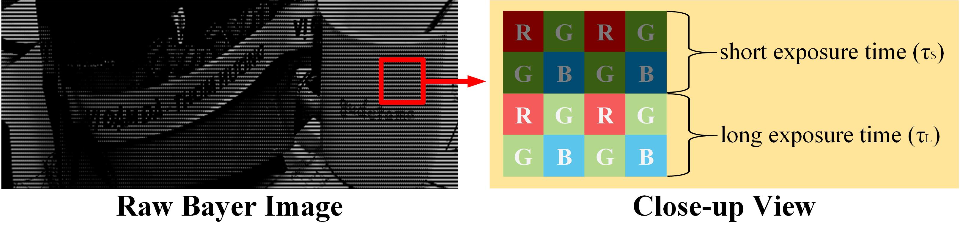
Figure 1: Raw Bayer image with row-wise varying exposure times [13].

Due to the challenge of ghosting removal [10, 11], ghosting artifacts are believed to be the Achilles’ heel for the exposure stacking-based HDRI. As such, exposure stacking is unsuitable for capturing HDR videos [14, 15, 16]. The single-shot HDRI was proposed to capture ghost-free HDR images with varying exposures in a single image [17, 13, 18, 19]. In the single-shot HDRI, the exposure of pixels varies along with different spatial locations.

In general, the raw data obtained by the camera is in a Bayer image. One typical example is given in Fig. 1, where the raw Bayer image is sensed by alternating the exposure time every other rows. This shooting method [20, 21, 13] is referred to as dual-time in this paper. In addition, the single-shot HDRI is also a good candidate to capture HDR videos [22].

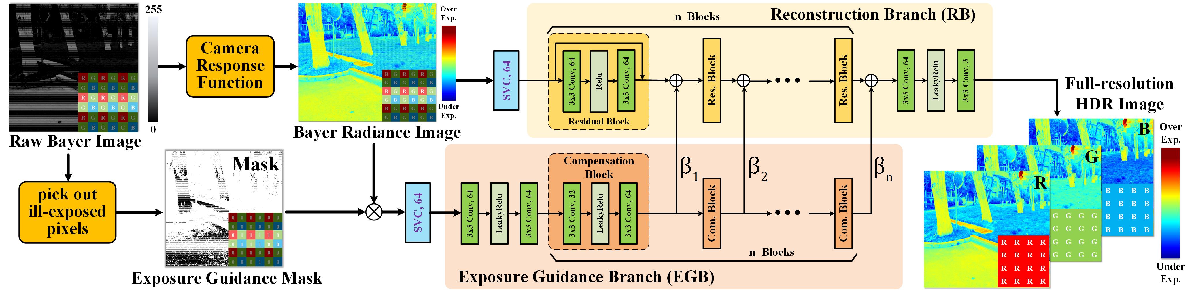
Figure 2: Overall framework of the proposed algorithm. The proposed CNN includes a reconstruction branch (RB), and two distinctive components: spatially varying convolution (SVC) and exposure-guidance branch (EGB).

Among the single-shot dual-time HDRI algorithms [20, 21, 13], the stages of demosaicing and HDR reconstruction are separated. Thus, the error generated in the previous stage will affect the posterior one, resulting in error accumulation and drift. Recently, the idea of joint demosaicing with other low-level image processing tasks [23, 24, 25, 26, 27] has appeared in some studies to avoid the cumulative error. However, the existing joint demosaicing algorithm’s convolution methods have not been adjusted accordingly to the spatial change of the data pattern. Moreover, when the captured Bayer image with varying exposure times is converted into a Bayer radiance image [21, 13] by using camera response functions (CRFs) [28], the brightness difference caused by different exposure time can not be completely eliminated. The ill-exposed pixels in the Bayer radiance image will also interfere the convolutional neural network (CNN) [13].

In this paper, a one-stage CNN is proposed for the single-shot dual-time HDRI. As shown in Fig 2.This novel CNN can restore high-quality HDR image at the full resolution from a single Bayer radiance image with varying exposures, by which the problem of cumulative errors in [13, 21, 20] can be avoided. Two distinctive components are introduced into the CNN to handle the challenges in single-shot HDRI. For the challenges of processing image pixels with varying colors (caused by the Bayer pattern) and varying exposures (caused by the dual-time), a novel spatially varying convolution (SVC) is designed and introduced as the first layer of CNN. The proposed SVC is adaptive to both varying colors and varying exposures, and can extract information from the dual-time Bayer image efficiently. The SVC can be easily inserted into other networks to process the Bayer image with or without SVE, and can be redesigned into other flexible variants when the data pattern or SVE changes. For the challenge of processing ill-exposed pixels, a novel exposure-guidance method is proposed, and the method is inspired by the dual-branch network [29, 30]. By exposure-guidance method, the prior knowledge of ill-exposed pixels is exploited, and an exposure-guidance branch (EGB) is proposed to assist the CNN by incorporating this prior.

Clearly, both the SVC and the exposure-guidance method can improve the explain-ability of the proposed one-stage CNN. Moreover, a new HDR dataset is proposed in this paper. The proposed dataset consists of 500 pairs of images with short and long exposures, respectively. The varying exposures are achieved by changing the exposure time. Images with camera shaking or object movement are filtered out artificially. Finally, extensive experimental results demonstrate the effectiveness of the proposed algorithm.

Overall, the four major contributions of this paper are as follows:

• A one-stage CNN with an improved explain-ability is proposed to address the problems of demosaicking and single-shot dual-time HDRI end-to-end..

• A novel SVC is introduced to process the Bayer image with or without SVE appropriately.

• An exposure-guidance method is proposed to reduce the interference of ill-exposed pixels.

• A new HDR dataset is proposed in this paper. Camera parameters for shooting are provided in detail for other related HDR researchers to use.

The rest of this paper is organized as follows. Relevant works are reviewed in Section II. Details of the proposed algorithm are presented in Section III. Extensive experimental results are provided in Section IV. Lastly, concluding remarks are listed in Section V.

II Literature Review

In this section, the relevant works on HDRI and demosaicing are reviewed.

II-A HDRI

II-A1 stack-based HDRI

The most popular method for generating an HDR image is to capture multiple differently exposed LDR images and merge all the LDR images into one HDR image. Such a method is called stack-based HDRI [31, 32, 33, 34]. All the captured LDR images are firstly mapped into the corresponding radiance maps through the CRFs [28], and multiple radiance maps are then fused into an HDR image via a weighted average manner.

Exposure stacking-based methods often perform well in static scenes. Nevertheless, in dynamic scenes, the positions of moving objects in the exposure stack are different, resulting in ghost artifacts in HDR images. To remove the ghosting artifacts, one of the input images is selected as the reference image. All moving objects in other images are synchronized with those objects in the reference images. Ghost removal was widely studied, and many interesting algorithms were introduced [35, 36, 37, 9, 12, 4]. However, when complex motion or extreme dynamic range occurs in the scene, all these algorithms could fail. As indicated in [10, 11], no universal deghosting algorithm is available. Ghosting artifacts are thus believed to the Achilles’ heel for the exposure stacking-based HDRI.

II-A2 Single-Shot HDRI

An alternative solution is to obtain multiple exposure information of a scene via a single shot, and this solution is attractive for HDR videos [22] and full light field reconstruction [38]. Nayar and Suda proposed the concept of spatially varying exposure (SVE) in [17, 19], such that diverse pixel values of a single image are differently exposed. Two types of typical methods can be adopted to achieve SVE.

One type is to change the ISO value at different positions of the sensor. Given an ISO-based SVE image, a few methods were proposed to restore the final HDR image, including the adaptive kernel regression-based method [39], inpainting-based deinterlacing method [40], joint learning-based method [41], dictionary-based method [42], adaptive filter-based method [43], and deep learning-based method [18]. Nevertheless, the increase in ISO for a high exposure will amplify the camera noise, especially in low-lighting conditions.

The other way to achieve SVE is to change exposure times [44, 13, 21, 20], in which higher-quality images than the ISO-based approach can be obtained, as indicated in [28]. For example, an image can be shot with the exposure times varying every other lines, as shown in Fig. 1. Gu et al. proposed to adopt the structure of a coded rolling shutter as the readout structure of a CMOS image sensor [20] and introduced several coding schemes and corresponding applications. Cho et al. designed a multistage processing flow to restore dual-time SVE Bayer images to HDR images gradually [21]. An and Lee introduced an CNN-based technology to correct Bayer images, and then adopted demosaicing to obtain HDR images [13].

The stages of HDR reconstruction and demosaicing are separated. Thus, the error generated in the previous stage will affect the posterior one, resulting in error accumulation and drift. In addition, to deal with the ill-exposed pixels in the Bayer radiance image, Cho et al. [21] completes the image by deleting ill-exposed pixels and then interpolating from neighbors. An et al. [13] takes the complete image as input and use CNN to correct ill-exposed pixels. Compared with [21], the CNN is allowed to make full use of the information in the Bayer radiance image [13, 44], but ill-exposed areas will also interfere with the imaging results of well-exposed areas during the calculation process.

II-B Image Demosaicing

A color filter array (CFA) is put in front of a CMOS sensor to use a sensor designed for grayscale images and capture color images [45]. Each pixel on a Bayer image taken in this way has only one of red, green, and blue. The image is subjected to a postprocessing algorithm called demosaicing, which is to complete the missing information in the Bayer image. In images without SVE, no brightness difference caused by the different exposures occurs. Existing demosaicing algorithms are divided into two categories: model-based [46, 47, 48, 49] and learning-based [23, 24, 23, 25, 26, 27].

To complete the missing two-thirds of pixels in the Bayer image, conventional model-based demosaicing algorithms [46, 47, 48, 49, 50] usually adopt different interpolation schemes for different data patterns. In learning-based demosaicing [23, 24, 25, 26, 27, 51] the missing pixels are interpolated by CNN. However, existing deep learning-based algorithms share a contrary interpolation philosophy with conventional demosaicing algorithms. As indicated by [52], the interpolators should be adaptive to the changing of data pattern. It is unreasonable to adopt a single same interpolation scheme for all data patterns, because missing colors that need to be interpolated vary with different data patterns. Thus, it is the same for deep learning, where different data patterns should be convolved by different convolution kernels, and same patterns by same convolution kernels. But their convolution method [23, 24, 25, 26, 27] has not been adjusted accordingly due to the spatial change of the data pattern.

Moreover, in the Bayer image with SVE, the CRFs cannot completely eliminate the brightness difference caused by different exposures times. Restoring an HDR image from a dual-time SVE Bayer image brings more challenges to demosaicing.

III Proposed Algorithm

Given a raw Bayer image captured within a single shot, the CRFs are firstly applied to generate the Bayer radiance image, and then the exposure-guidance mask is generated from a raw Bayer image. The Bayer radiance image is restored into an HDR radiance map via a novel CNN end-to-end, and the prior information in the exposure-guidance mask can assist the CNN. Then the CNN includes a reconstruction branch (RB), and two distinctive components: spatial varying convolution (SVC) and exposure-guidance method. Both the proposed SVC and exposure-guidance method make the CNN more explainable. The overall joint learning framework is shown in Fig. 2. It should be pointed out that the proposed algorithm is on top of our previous work [53].

III-A Generation of Bayer Radiance Image

The raw input image $Z$ captured within a single shot is a N-bit (N can be 8, 10, 12, etc.) Bayer image with row-wise varying exposure times [13, 21, 20], as shown in Fig. 1. Let $\Delta t_{ij}$ be the exposure time of the pixel in the $i$th row, $j$th column of $Z$, then it is given as:

$$\Delta t_{ij}=\begin{cases}{\tau_{S},}&{i\bmod 4=1\;{\rm or}\;2}\\ {\tau_{L},}&{i\bmod 4=3\;{\rm or}\;0}\end{cases},$$ (1)

where $\tau_{S}$ and $\tau_{L}$ are the short and long exposure times, respectively.

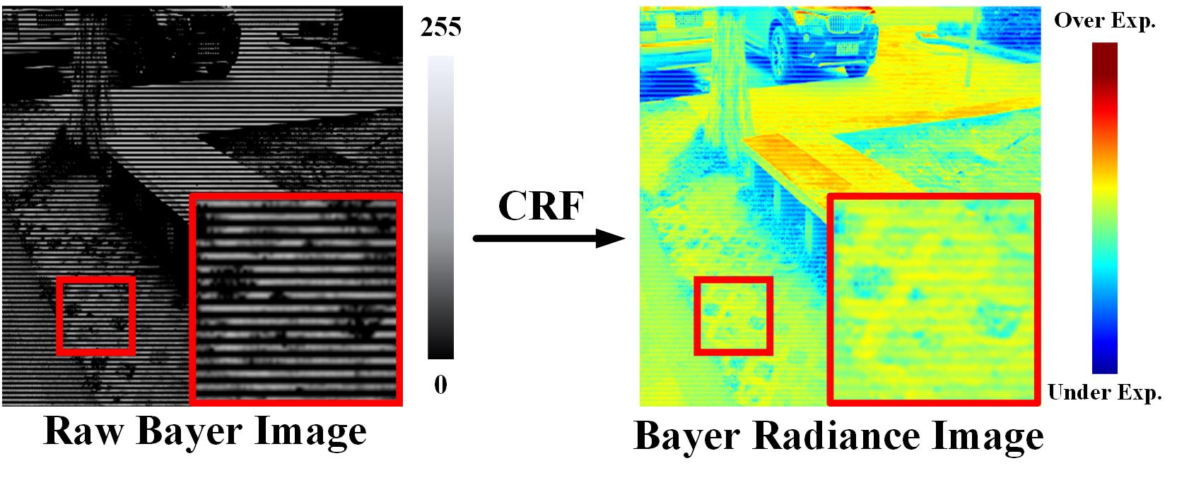
Figure 3: Brightness differences are partly reduced using CRF. The slight horizontal stripes represent that the brightness differences cannot be completely eliminated.

To restore the corresponding HDR image, the Bayer image $Z$ is firstly converted into a Bayer radiance image $E$ [13]. The pixel $z_{ij}$ of $Z$ is normalized according to its exposure time.

$$\ln(e_{ij})=\ln(f_{c_{ij}}^{-1}(z_{ij}))-\ln(\Delta t_{ij}),$$ (2)

where $c_{ij}\in\{R,G,B\}$ is the color channel of $z_{ij}$. The CRF $f_{c_{ij}}(\cdot)$ can be estimated via the method in [28]. $f_{c_{ij}}^{-1}(\cdot)$ is the inverse function of $f_{c_{ij}}(\cdot)$. $e_{ij}$ represents the converted irradiance pixel. Note that CRFs are assumed to be available, because they can be easily estimated for any digital cameras and smartphones. As shown in Fig. 3, the brightness differences caused by the dual-time are partially reduced.

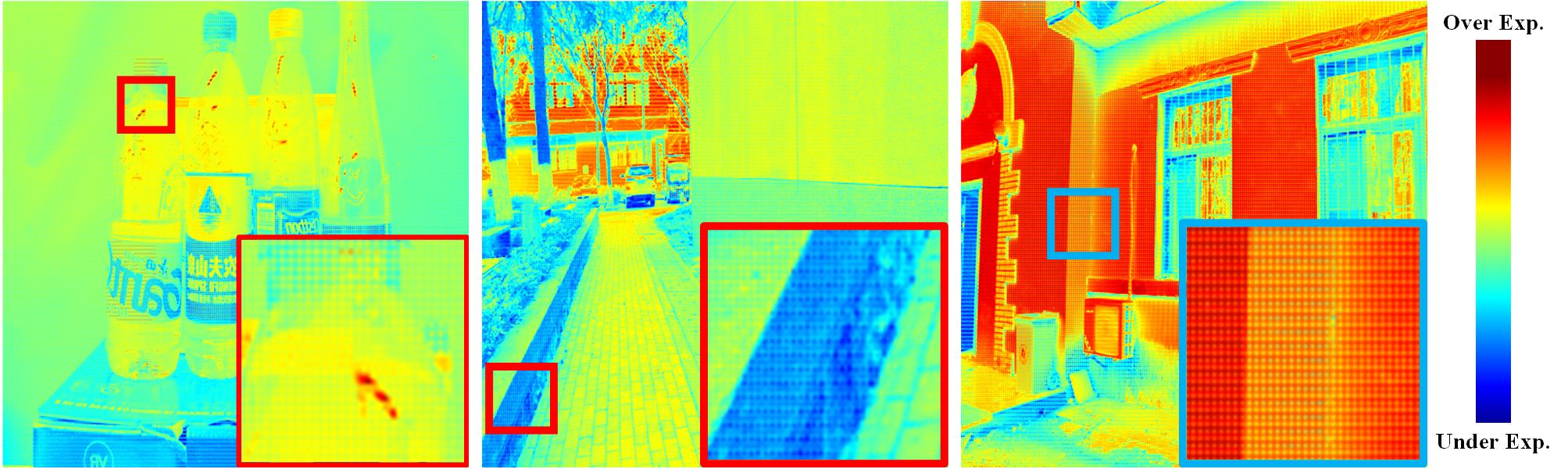
Figure 4: Since only a single color (R, G, or B) is recorded at each pixel position, the visible grids appear in the Bayer radiance image.

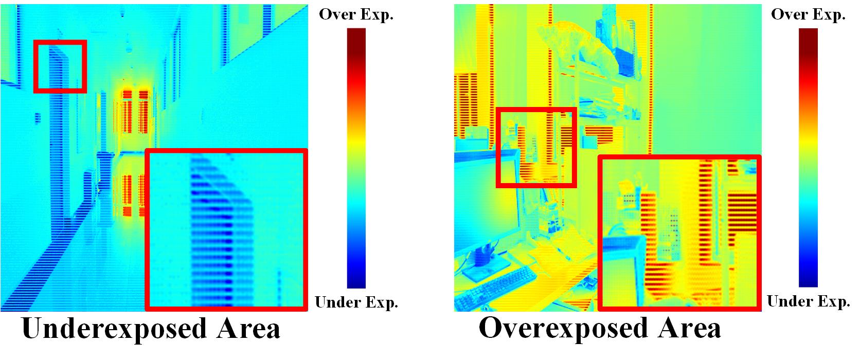
Figure 5: Horizontal stripes indicating poor information, which is caused by over- and under-exposure.

As indicated above, there are three main challenges in restoring a full-resolution HDR image from a dual-time Bayer radiance image. First, two-thirds of color pixels are missed, resulting in visible grids, as shown in Fig. 4. Second, the remaining pixels are carried with varying exposures and the brightness differences cannot be completely eliminated via CRFs, like the horizontal stripes shown in Fig. 3. Moreover, some of the captured pixels are ill-exposed, which makes the HDR restoration more difficult, as shown in Fig. 5.

III-B Spatially Varying Convolution

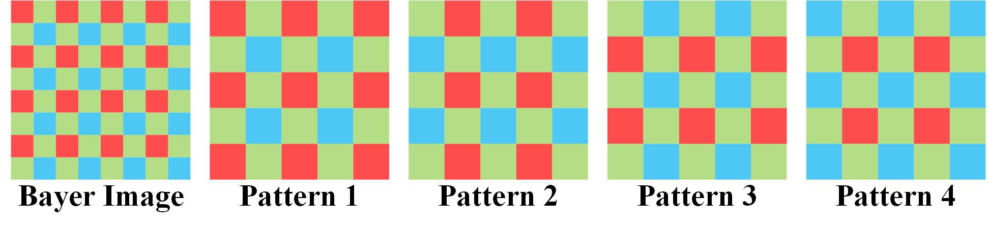
Figure 6: Illustration of four different patterns in a $5\times 5$ receptive field

There are four color patterns in the Bayer image, as shown in Fig. 6. Conventional demosaicing methods complete pixels via color pattern-oriented interpolation schemes [46, 54, 55], which means that there exist different interpolators corresponding to the four different color patterns. However, demosaicing has not been adjusted accordingly across various color patterns in existing deep learning-based methods [24, 25, 26, 27]. All color patterns in an image are interpolated by a same kernel slidingly. It is difficult to realize adaptive interpolation due to weights sharing in the convolution.

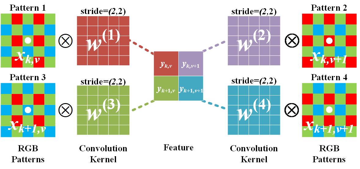
Figure 7: Illustration of four different RGB patterns in a $5\times 5$ receptive field, and the corresponding degraded version of spatially varying convolution (SVC-D).

We proposed a novel convolution method to use incomplete weight sharing for sliding kernels, which is called spatial varying convolution (SVC) [53]. In the SVC, the kernel weights are shared across the same patterns but different across different patterns. Considering the four color patterns in Fig. 6, at least four different kernels need to be included in the SVC, as shown in Fig. 7.

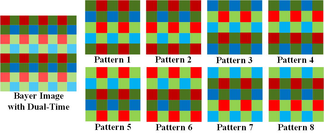
Figure 8: Illustration of eight different patterns in a $5\times 5$ receptive field, where the darker and lighter colors represent the short and long exposed radiation pixels, respectively.

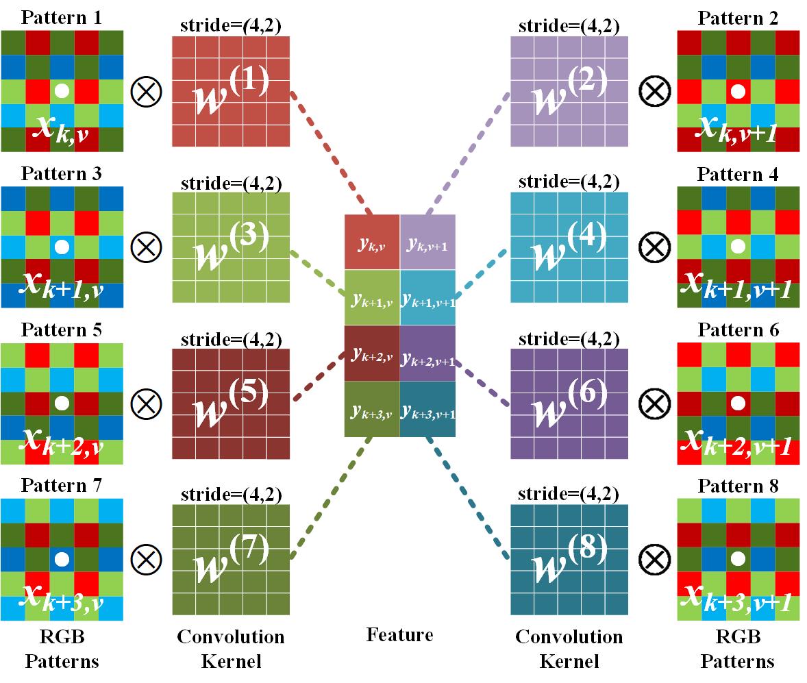
Figure 9: Illustration of spatially varying convolution (SVC) based on 8 patterns.

Our proposed SVC [53] is extended to a more complicated scenario. In a Bayer image captured by the dual-time shooting, the exposure time also varies along with image pixels. As shown in Fig. 3, the brightness differences, caused by the varying exposure times, cannot be eliminated by converting a Bayer image into a Bayer radiance image via the CRFs. Considering both varying colors and varying brightness, there are totally eight patterns in a $5\times 5$ receptive field, as shown in Fig. 8. The darker and lighter colors represent the short and long exposed radiation values, respectively. Therefore, to adapt better to more kinds of patterns, the SVC is modified into a more complicated version, which includes eight interpolation kernels overall, as shown in Fig. 9. The improved SVC is more robust to the varying patterns in a dual-time Bayer image. The details of the improved SVC are given in the following text.

Let $x_{k,v}$ and $y_{k,v}$ be the pixels at position $(k,v)$ in the input and output of SVC, respectively. $w^{(1)}$, $w^{(2)}$, $w^{(3)}$, $w^{(4)}$, $w^{(5)}$, $w^{(6)}$, $w^{(7)}$, and $w^{(8)}$ represent different convolution kernels. The proposed SVC is then defined as follows:

$$\small{\begin{cases}{y_{k,v}}&=\sum\limits_{i=-2}^{2}{\sum\limits_{j=-2}^{2}{(w^{(1)}_{i,j}\times x_{k+i,v+j})}}\\ {y_{k,v+1}}&=\sum\limits_{i=-2}^{2}{\sum\limits_{j=-2}^{2}{(w^{(2)}_{i,j}\times x_{k+i,v+1+j})}}\\ {y_{k+1,v}}&=\sum\limits_{i=-2}^{2}{\sum\limits_{j=-2}^{2}{(w^{(3)}_{i,j}\times x_{k+1+i,v+j})}}\\ {y_{k+1,v+1}}&=\sum\limits_{i=-2}^{2}{\sum\limits_{j=-2}^{2}{(w^{(4)}_{i,j}\times x_{k+1+i,v+1+j})}}\\ {y_{k+2,v}}&=\sum\limits_{i=-2}^{2}{\sum\limits_{j=-2}^{2}{(w^{(5)}_{i,j}\times x_{k+2+i,v+j})}}\\ {y_{k+2,v+1}}&=\sum\limits_{i=-2}^{2}{\sum\limits_{j=-2}^{2}{(w^{(6)}_{i,j}\times x_{k+2+i,v+1+j})}}\\ {y_{k+3,v}}&=\sum\limits_{i=-2}^{2}{\sum\limits_{j=-2}^{2}{(w^{(7)}_{i,j}\times x_{k+3+i,v+j})}}\\ {y_{k+3,v+1}}&=\sum\limits_{i=-2}^{2}{\sum\limits_{j=-2}^{2}{(w^{(8)}_{i,j}\times x_{k+3+i,v+1+j})}}\\ \end{cases},}$$ (3)

where $k=0,4,8,...,4n_{1}\leq H$, and $v=0,2,4,...,2n_{2}\leq W$. $H$ and $W$ are the height and width of input or output, respectively. Benefiting from the SVC, the data pattern is the same for each convolution kernel, which can reduce the burden of network learning. The proposed SVC is one distinctive component of the proposed CNN.

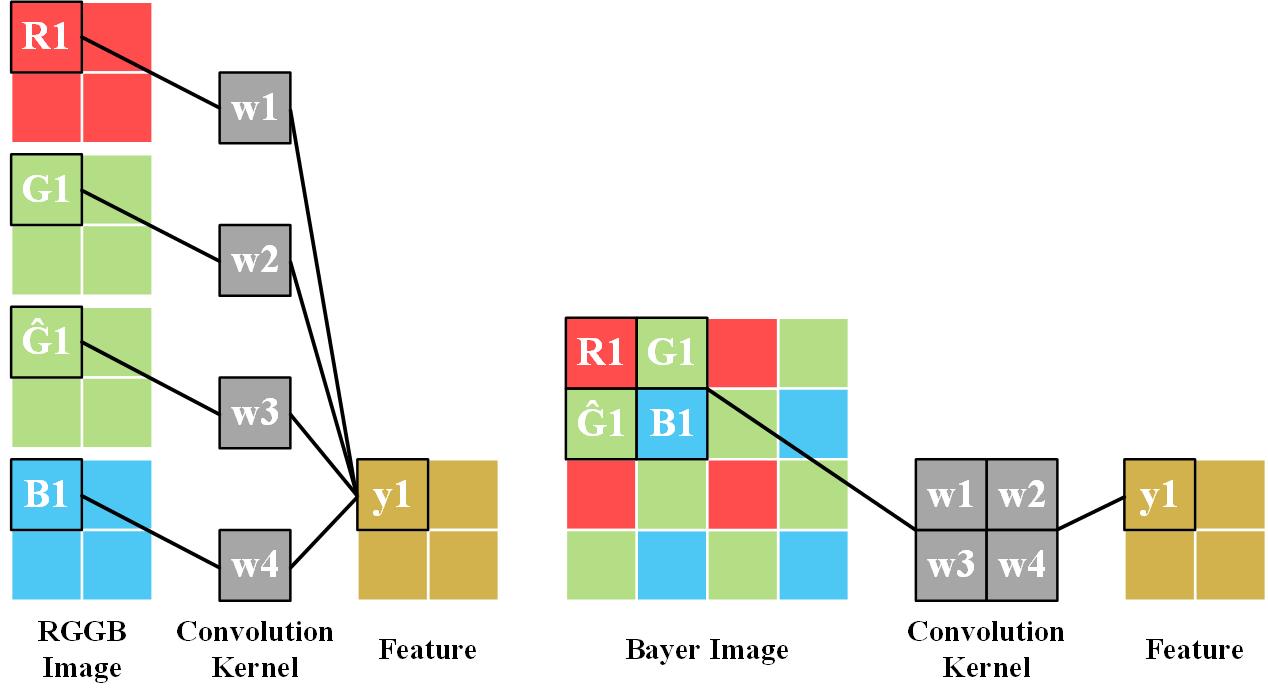
Figure 10: Illustration of convolving an RGGB image which uses $1\times 1$ convolution kernels at stride 1, and convolving a Bayer image which uses $2\times 2$ convolution kernels at stride 2. The two operations are equivalent.

Note that the difference between the SVC and existing methods is whether it is the convolution with complete weight sharing. Specifically, considering the algorithm in [24], the Bayer image is convolved at stride 1. The convolutional kernel receives four kinds of patterns during sliding, as shown in Figure 6. According to the principle of convolution, kernel weights are shared, by which different data patterns are convolved by the same convolutional kernels. Existing CNN-based demosaicing algorithms adopt two methods. One method is to set the stride as 2 or 4 [25], by which the kernel receives only one kind of data pattern. Another method is to rearrange the single-channel Bayer image into a four-channel RGGB image, whose length and width are reduced by half. Then the rearranged image is convolved with a stride of 1 [26, 27]. The above two methods are actually equivalent. For example, convolving an RGGB image with a $1\times 1$ kernel at stride 1 is equivalent to convolving a Bayer image with a $2\times 2$ kernel at stride 2, as shown in Fig. 10. Both methods focus on interpolating only one kind of data pattern, where the other three kinds of patterns are not considered. While, the SVC can be adjusted accordingly to the spatial change of the data pattern.

Moreover the SVC can have flexible variants when the data pattern and SVE changes. The SVC is only used in the first layer of CNN, as shown in Fig. 2. Thus, compared to the weight-sharing convolution method, the SVC improves the imaging ability of CNN via minimal additional parameters.

III-C Reconstruction Branch

The reconstruction branch (RB) shares a similar philosophy to the networks utilized in image-to-image translation tasks, such as image demosaicing [56], super-resolution imaging [57], and image denoising [58]. The RB is composed of several residual blocks, as shown in Fig. 2. Each block is realized by an operation of convolution–ReLu–convolution and an identical mapping. Specifically, the kernel size in each convolutional layer is set to $3\times 3$. The stride and padding are both set to 1 to maintain the feature resolution during propagation. The structure of RB is shown in Fig. 2.

III-D Exposure-Guidance Method

Over- and under-exposed areas exist in the rows with long- and short-exposure times, respectively. These ill-exposed areas are usually dominated by saturation noise. These areas lead to unreliable and poor information in the radiance map $E$, which turns into visible boundaries at the corresponding pixel positions, as shown in Fig. 5. These ill-exposed areas can interfere with the CNN and are thus desired to be detected. To overcome this, an exposure-guidance method is proposed, which consists of exposure guidance mask and exposure guidance branch (EGB). The exposure-guidance method is the other distinctive component of the proposed CNN.

III-D1 Exposure-Guidance Mask

In conventional HDRI algorithms [9, 12, 5, 13] , a threshold value is usually predefined on a N-bit image to identify the ill-exposed pixels. To simulate this artificial selection in a CNN-based algorithm, a exposure-guidance mask $M$ is computed using the following equation:

where the $m_{ij}$ is the value at position $(i,j)$ in $M$. N is the number of bits for the input image and $\alpha$ is a percentage constant. Note that $M$ has the same size as $Z$ and $E$. Then, $M$ can be easily fed into the network along with the radiance map $E$, which can be considered as a prior of knowledge to help the network know which area is ill-exposed. Based on the rule of thumb in [13] and the sensitivity analysis of $\alpha$ in Section IV-C, threshold value $\alpha$ is empirically selected as $3.92\%$.

III-D2 Exposure-Guidance Branch

The mask can be concatenated or element-wise multiplied with a Bayer radiance image as the network input, providing auxiliary prior information. However, the features of the radiance map are not guided by the mask in a deep-level manner because of this early fusion. Inspired by [29, 30], an EGB is proposed to guide the HDR reconstruction as an auxiliary branch, as shown in Fig. 2. Prior information can be extracted by this branch, which makes the CNN explainable.

During propagation, the exposure-guidance mask is first multiplied with the Bayer radiance image $E$. Thus, the poor information from the ill-exposed area will be filtered out, such that the EGB will tend to utilize the features extracted from the well-exposed area. Then, the features of the EGB are embedded into the RB in a multilevel manner to realize compensation, in which information is fused in a deeper level. Finally, the network can pay considerable attention to the well-exposed areas, which provide accurate HDR information.

The proposed EGB consists of $n$ blocks, and each block includes two convolutional layers and an activation layer. To reduce the computational cost, the output channels of the first convolutional layer are compressed in each block.

$E$ can be simply multiplied by $M$ as the input of RB to make the network focus on the well-exposed areas only. The experimental results in Section IV-C show that this method does not work as expected. The possible reason is that the raw Bayer pattern is destroyed, and the irregular data makes the network difficult to deal with.

III-E Loss Function

The $L_{1}$ loss function is widely used in deep learning-based low-level image processing [59], and it is formalized as

$$\mathcal{L}_{l1}=\frac{1}{3\times H\times W}\sum\limits_{i=1}^{H}{\sum\limits_{j=1}^{W}{|\boldsymbol{r}_{ij}-\tilde{\boldsymbol{r}}_{ij}|}},$$ (5)

where $\boldsymbol{r}_{ij}$ and $\tilde{\boldsymbol{r}}_{ij}$ represent two 3D $(R,G,B)$ vectors at position $(i,j)$ in the image. The resolution of the ground truth $R$ and generated HDR image $\widetilde{R}$ is $H\times W$.

To reduce the color deviation between $R$ and $\widetilde{R}$, the color loss $\mathcal{L}_{c}$ is introduced as follows [60]:

$$\mathcal{L}_{c}=\frac{1}{H\times W}\sum\limits_{i=1}^{H}{\sum\limits_{j=1}^{W}{(1-cos(\boldsymbol{r}_{ij},\tilde{\boldsymbol{r}}_{ij}))}},$$ (6)

where $cos(\boldsymbol{r}_{ij},\tilde{\boldsymbol{r}}_{ij})$ represents the cosine similarity of $\boldsymbol{r}_{ij}$ and $\tilde{\boldsymbol{r}}_{ij}$. $\mathcal{L}_{c}$ is sensitive to color difference. The overall loss function is given as

$$\mathcal{L}_{total}=\mathcal{L}_{l1}+\lambda\mathcal{L}_{c},$$ (7)

where $\lambda$ is a constant, and its value is selected as 0.1.

IV Experimental Results

IV-A Implementation Details

IV-A1 Datasets Description

Experiments are conducted on two datasets, VETHDR-Nikon dataset and VETHDR-Canon dataset, where the different exposures are achieved by varying the exposure times (VET) instead of changing the ISO. 500 pairs of images are included in each dataset. Each pair consists of two full-resolution images $I_{L}$ and $I_{S}$, with long and short exposure times, respectively. The exposure time ratio and ISO are fixed as 16 and 800, during shooting respectively. All the images are resized to $480\times 480$. Among each of the dataset, 300 pairs are used for training, 100 pairs for validation and 100 pairs for test. To simulate the input dual-time Bayer image $Z$, the pixels on every two rows are alternatively sampled from $I_{S}$ and $I_{L}$. The ground-truth HDR image $Y$ is obtained by merging the full-resolution images $I_{S}$ and $I_{L}$ via the method of [28].

The VETHDR-Nikon dataset is from [61, 62], collected by a Nikon 7200 camera. It consists of original images in 8-bit color JPEG files format. The corresponding CRF [28] is recorded in the dataset. The Bayer Radiance Image can be calculated from the raw input image $Z$ through the nonlinear CRF.

The VETHDR-Canon dataset is collected by a Canon 5D4 camera in this paper. It contains 16-bit color images with the original digital counts for each of the RGB channels, which are generated from the 16-bit RAW image files by the method in [63]. Since the RAW files typically have a nearly linear CRF, the Bayer Radiance Image can be calculated from the raw input image $Z$ through a simple linear transformation.

IV-A2 Comparison Description

In terms of qualitative comparison, the results are visualized by sequentially executing the tone mapping algorithm [64] and the white balance algorithm [65] on the radiance map. In terms of quantitative comparison, we choose HDR-MAE, HDR-MSE, HDR-VDP, HDR-PSNR-RGB, HDR-SSIM-RGB, HDR-PSNR-Y, and HDR-SSIM-Y as the evaluation metrics. These metrics are measured on the radiance maps. For the HDR-MAE and HDR-MSE, lower is better. For the HDR-VDP, HDR-PSNR-RGB, HDR-SSIM-RGB, HDR-PSNR-Y, and HDR-SSIM-Y, higher is better. Among them, a perceptually uniform (PU) encoding [66] is utilzed to enable PSNR and SSIM to be used to evaluate the quality of HDR images. In addition, the model parameters (P) and the floating-point operations (FLOPs) are provided as reference. All evaluation metrics are calculated on the HDR radiance image, and which are explained as follows:

• HDR-MAE: The average absolute value based on the PU encoding, which calculates the difference between the test image and the reference image.

• HDR-MSE: The average square value based on the PU encoding, which calculates the difference between the test image and the reference image.

• HDR-VDP: A high dynamic range visible difference predictor in version 2.2.2. Its quality correlate score can be used to evaluate image differences [67].

• HDR-PSNR-RGB: Peak signal-to-noise ratio based on the PU encoding, which calculates the difference of the image in the R, G, and B channels.

• HDR-SSIM-RGB: Structural similarity [68] based on the PU encoding, which calculates the difference of the image in the R, G, and B channels.

• HDR-PSNR-Y: Peak signal-to-noise ratio based on the PU encoding, which calculates the difference of the image in the Y channel.

• HDR-SSIM-Y: Structural similarity [68] based on the PU encoding, which calculates the difference of the image in the Y channel.

• P: Number of parameters in CNN.

• FLOPs: The number of floating-point operations required for network to generate an image.

IV-A3 Training Details

The RB and EGB are realized using 16 blocks. We randomly sample $128\times 128$ patch from each input during training. We set the batch size and the number of iterations to 16 and $2\times 10^{5}$, respectively. We set $\lambda$ in Equation (7) to 0.1. The Adam optimizer with $\beta_{1}=0.9$ and $\beta_{2}=0.99$ is used for optimization. The learning rate is initially set as $2\times 10^{-4}$ and finally decreased to $1\times 10^{-7}$ through a cosine annealing schedule. Each model is trained on an NVIDIA GTX 1080Ti GPU for approximately two days. All the experiments are implemented using PyTorch.

IV-B Analysis of SVC

To demonstrate the effectiveness of the SVC, we compare the SVC with many other alternative methods qualitatively and quantitatively. We also perform a quantitative comparison of SVCs with different convolution kernel sizes.

IV-B1 Alternative Methods

TABLE I: Summary of various convolutional layers for Bayer images in existing algorithms.

Method	Opt-base	Opt-2-2 [24]	Opt-4-2 [25]	Opt-4-4 [25]	Opt-RGGB [26, 27]
Input Shape	$h\times w\times 1$	$h\times w\times 1$	$h\times w\times 1$	$h\times w\times 1$	$\frac{h}{2}\times\frac{w}{2}\times 4$
Kernel Size	$3\times 3$	$2\times 2$	$4\times 4$	$4\times 4$	$3\times 3$
Stride	(1,1)	(2,2)	(2,2)	(4,4)	(1,1)
Upsampling Layer	Unused	2	2	4	2
Output Shape	$h\times w\times 64$	$h\times w\times 64$	$h\times w\times 64$	$h\times w\times 64$	$h\times w\times 64$

The SVC is a flexible solution for processing a dual-time Bayer image, which ensures that pixels of different color patterns are convolved using different kernels. When the varying exposures caused by the dual-time are not considered, the SVC can be degraded to SVC-D [53]. We further increase the kernel size of SVC-D to $5\times 5$, as shown in Fig. 7. The SVC-D is equivalent to adding the following conditions to Equation (3).

$$\begin{cases}w^{(1)}_{i,j}=w^{(5)}_{i,j}&w^{(2)}_{i,j}=w^{(6)}_{i,j}\vspace{1ex}\\ w^{(3)}_{i,j}=w^{(7)}_{i,j}&w^{(4)}_{i,j}=w^{(8)}_{i,j}\\ \end{cases},$$ (8)

In addition to the proposed SVC and SVC-D in this paper, a few special convolutional layers in deep learning have been utilized to process a special Bayer image in advance [24, 25, 26, 27]. All these layers/methods are summarized in Table I. The first column indicates the method characteristics, which are explained as follows:

• Input Shape: The shape of the input Bayer image, including the height, width, and number of channels.

• Kernel Size: The size of kernel in the first convolutional layer.

• Stride: The stride during kernel sliding in the first convolutional layer, including the vertical and horizontal strides.

• Upsampling Layer: The upsampling layer is realized by the sub-pixel convolution [69]. 2 and 4 indicate the scaling factor.

• Output Shape: The shape of the output produced by the first convolutional layer, including the height, width and number of channels.

Table I presents that two types of convolutional layers can be used for processing a Bayer image. One type is that a convolution kernel of even size extracts the color information with a stride of even. Then, the downsampled output is resized to the original resolution by using the upsampling layer, such as Opt-2-2 [24], Opt-4-2 [25], Opt-4-4 [25], and Opt-RGGB [26, 27]. Overall, all these convolutional layers are designed toward the same goal, i.e., to make the color pattern convolved using the kernel be the same. Opt-base represents the general convolutional layer with a kernel size of $3\times 3$.

TABLE II: Quantitative comparison among the baseline, existing operations, and our SVC. The best results are shown in bold, and the second-best results are shown in blue. The results come from the VETHDR-Nikon test set.

Method	HDR-MAE	HDR-MSE	HDR-VDP	HDR-PSNR-RGB	HDR-SSIM-RGB	HDR-PSNR-Y	HDR-SSIM-Y	P [$10^{6}$]	FLOPs [$10^{11}$]
Opt-base	2.982	53.874	65.59	41.38	0.9786	43.99	0.9860	1.221	2.813
Opt-2-2	2.911	41.480	65.72	41.72	0.9787	44.12	0.9859	1.222	2.813
Opt-4-2	2.962	42.596	65.55	41.61	0.9782	44.02	0.9856	1.225	2.814
Opt-4-4	2.983	41.916	65.57	41.62	0.9783	44.00	0.9856	1.238	2.814
Opt-RGGB	2.903	41.159	65.68	41.79	0.9788	44.20	0.9859	1.230	2.817
SVC-D	2.889	40.744	65.74	41.84	0.9790	44.21	0.9860	1.227	2.816
SVC	2.881	40.052	65.69	41.91	0.9791	44.33	0.9861	1.234	2.816

The convolutional layers in Table I are combined with the RB to compare their performance. The results of 7 evaluation metrics on the radiance map are reported in Table II. The number of parameters is also provided as reference. The SVC and SVC-D surpass other convolutional layers, which demonstrates that the network learning can be affected by the varying color patterns and the SVC is a more robust solution. Moreover, the leading performance of SVC over SVC-D can prove the necessity of further consideration of brightness difference in a dual-time Bayer image.

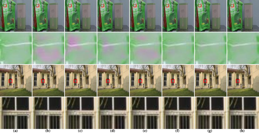
Figure 11: Qualitative comparison among the baseline, existing convolutional layers, and our SVC. (a) Ground truth, (b) Opt-base, (c) Opt-2-2, (d) Opt-4-2, (e) Opt-4-4, (f) Opt-RGGB, (g) SVC-D, (h) SVC. The results come from the VETHDR-Nikon test set.

The qualitative results are shown in Fig. 11. In the first row, (b), (c), (d), (e), and (f) fail in estimating correct colors. In the second row, clearer edges are recovered using (h), whereas other results have different degrees of blurring on edges. The SVC can make the network restore correct colors and textures.

IV-B2 Kernel Size

TABLE III: Quantitative comparison among SVC-3, SVC-5, and SVC-7. The best results are shown in bold, and the second-best results are shown in blue. The results come from the VETHDR-Nikon test set.

Method	HDR-MAE	HDR-MSE	HDR-VDP	HDR-PSNR-RGB	HDR-SSIM-RGB	HDR-PSNR-Y	HDR-SSIM-Y	P [$10^{6}$]	FLOPs [$10^{11}$]
Baseline	2.982	53.874	65.59	41.38	0.9786	43.99	0.9860	1.221	2.813
SVC-3	2.941	40.809	65.70	41.80	0.9788	44.19	0.9859	1.225	2.813
SVC-5	2.881	40.052	65.69	41.91	0.9791	44.33	0.9861	1.234	2.816
SVC-7	2.902	40.548	65.68	41.87	0.9790	44.28	0.9860	1.246	2.819

The SVCs with different kernel sizes are also experimented. In Table III, SVC-3, SVC-5, and SVC-7 indicate a kernel size of $3\times 3$, $5\times 5$, and $7\times 7$, respectively. All the SVCs outperform the original convolution (Opt-base). It can be seen that simply increasing the kernel size of SVC brings little gains on performance. Thus, the power of SVC lies in the design philosophy, not the increasing parameters.

IV-C Analysis of Exposure Guidance

To demonstrate the effectiveness of the exposure-guidance method, we compare the exposure-guidance method with many other alternative methods qualitatively and quantitatively. We also perform a quantitative comparison of EGBs with different threshold values $\alpha$. Moreover, we analyze the working mechanism of EGB through feature map and $\beta_{i}$.

IV-C1 Alternative Methods

The exposure-guidance mask is necessary to incorporate into the main network RB by adopting the EGB. Besides the EGB, there are three other ways in incorporating the exposure-guidance mask. The first method is to multiply the exposure-guidance mask and the Bayer radiance image to obtain an input matrix with a size of $h\times w\times 1$, in which the value of ill-exposed pixels becomes 0. This matrix is directly fed into the main network RB. The second method is to concatenate the exposure-guidance mask with the Bayer radiance image to generate a $h\times w\times 2$ matrix, which is then fed into the RB. The third method is to use the exposedness-aware compensation branch (EACB) to achieve deep-level fusion of masks and features [53]. To make a fair comparison, for the first two method, we set the number of residual blocks in the RB as 25. For the third method and the EGB, we set both the number of blocks in RB and EGB as 16.

TABLE IV: Quantitative comparison between the baseline and four different methods of using exposure-guidance masks. The best results are shown in bold, and the second-best results are shown in blue. The results come from the VETHDR-Nikon test set.

Method	HDR-MAE	HDR-MSE	HDR-VDP	HDR-PSNR-RGB	HDR-SSIM-RGB	HDR-PSNR-Y	HDR-SSIM-Y	P [$10^{6}$]	FLOPs [$10^{11}$]
Baseline	2.982	53.874	65.59	41.38	0.9786	43.99	0.9860	1.221	2.813
Multiplication	3.314	87.445	64.74	40.42	0.9757	43.24	0.9843	1.886	4.345
Concatenation	2.904	50.018	65.75	41.50	0.9790	44.11	0.9862	1.886	4.346
RB+EACB [53]	2.900	48.224	65.68	41.54	0.9790	44.12	0.9862	2.072	4.773
RB+EGB	2.861	47.835	65.83	41.72	0.9794	44.32	0.9865	1.850	4.263

The 7 evaluation metrics on the test set are reported in Table IV. Among them, the result of the multiplication-based method is worst. This implies that the information is not utilized after resetting the ill-exposed pixels to 0. The raw RGB pattern in the Bayer image is destroyed, and the irregular data make the network difficult to learn. The concatenation-based method is improved compared with the baseline on the 7 evaluation metrics, indicating that the awareness of ill-exposed pixels can improve the performance. However, the prior of the exposure-guidance mask is not incorporated into the network in a deep-level way, in which the performance improvements are limited. The EACB [53] is able to incorporate the prior knowledge of ill-exposed pixels in the feature level. The proposed EGB is a modification of EACB and compensates the RB in a both multi-level and feature-level way. Since the EACB-based method [53] only compensates RB once at the deepest level, the lack of compensation times make the performance improvement less obvious than the concatenation-based method. The method of using the EGB achieves the best results on all four indicators, which strongly proves the effectiveness of fusing the prior in a deep- and multi-level way. The EGB can focus only on the well-exposed area, and can exploit accurate information for HDR reconstruction. This network structure design is also more explainable. Moreover, the original information of the dual-time Bayer image is preserved. The EGB also has the highest computational efficiency.

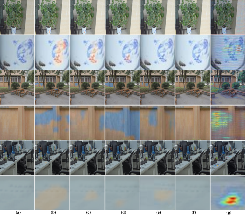
Figure 12: Qualitative comparison between the baseline and three different methods of using exposure-guidance masks. (a) Ground truth, (b) baseline, (c) the method of using multiplication, (d) the method of using concatenation, (e) RB+EACB [53], (f) RB+EGB, (g) overlay of EGB’s feature output and tone-mapped ground truth. The results come from the VETHDR-Nikon dataset.

The qualitative results are shown in Fig. 12. The EGB-based method performs evidently better on the four sets of images, whereas the other methods cause different degrees of unnatural color distortions.

TABLE V: $\beta$ in the trained RB+EGB.

$\beta_{1}$	$\beta_{2}$	$\beta_{3}$	$\beta_{4}$	$\beta_{5}$	$\beta_{6}$	$\beta_{7}$	$\beta_{8}$
0.6463	0.3757	0.6446	0.8103	0.7389	0.6234	0.4541	0.6906
$\beta_{9}$	$\beta_{10}$	$\beta_{11}$	$\beta_{12}$	$\beta_{13}$	$\beta_{14}$	$\beta_{15}$	$\beta_{16}$
0.5762	0.6027	0.6895	0.7473	0.8965	0.9381	0.9597	0.9734

IV-C2 Threshold Selection

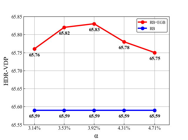
Figure 13: The HDR-VDP score of the models under different $\alpha$. The results come from the VETHDR-Nikon test set.

In order to observe the effect of different $\alpha$ on the EGB, we chose 5 values for testing. The selected values are all around the empirical value $3.92\%$ given in [13]. The HDR-VDP scores of RB+EGB and RB under different $\alpha$ are shown in Figure 13. It can be observed from the figure that the performance of EGB is less affected by the changing of $\alpha$, and all the scores of RB+EGB significantly surpass the baseline RB. This proves the robustness of the exposure-guidance method. Since the HDR-VDP score of RB+EGB is the highest when $\alpha=3.92\%$, $3.92\%$ is selected as the threshold.

IV-C3 Choice of Weight Function

TABLE VI: Quantitative comparison baseline and RB+EGB with three different weights. The best results are shown in bold, and the second-best results are shown in blue. The results come from the VETHDR-Nikon test set.

Method	HDR-MAE	HDR-MSE	HDR-VDP	HDR-PSNR-RGB	HDR-SSIM-RGB	HDR-PSNR-Y	HDR-SSIM-Y	P [$10^{6}$]	FLOPs [$10^{11}$]
Baseline	2.982	53.874	65.59	41.38	0.9786	43.99	0.9860	1.221	2.813
Robertson’s function [70]	2.926	42.686	65.86	41.66	0.9791	44.26	0.9863	1.850	4.263
Debevec’s function [28]	2.879	45.644	65.85	41.67	0.9790	44.35	0.9863	1.850	4.263
Our function	2.861	47.835	65.83	41.72	0.9794	44.32	0.9865	1.850	4.263

Equation (4) is compared with two commonly used weight functions, Debevec’s function [28] and Robertson’s function [70]. The results of the baseline and RB+EGB with three different weight functions are shown in Table VI. The RB+EGB improves significantly from the baseline no matter what weight functions are adopted. This demonstrates that the gains are mainly coming from the design of EGB. Compared with the weight functions in [28, 70], the Equation (4) achieves comparable performances. The simple and concise Equation (4) is selected as the final weight function.

IV-C4 Working Mechanism

The learned parameter $\beta$ in Fig. 2 is reported in Table V. All values are between 0.3757 and 0.9734, which means that the EGB provides useful information for the restoration of full-resolution HDR images. The $\beta$ tends to increase as the network deepens, indicating that the compensated information from the EGB is important in a deep level.

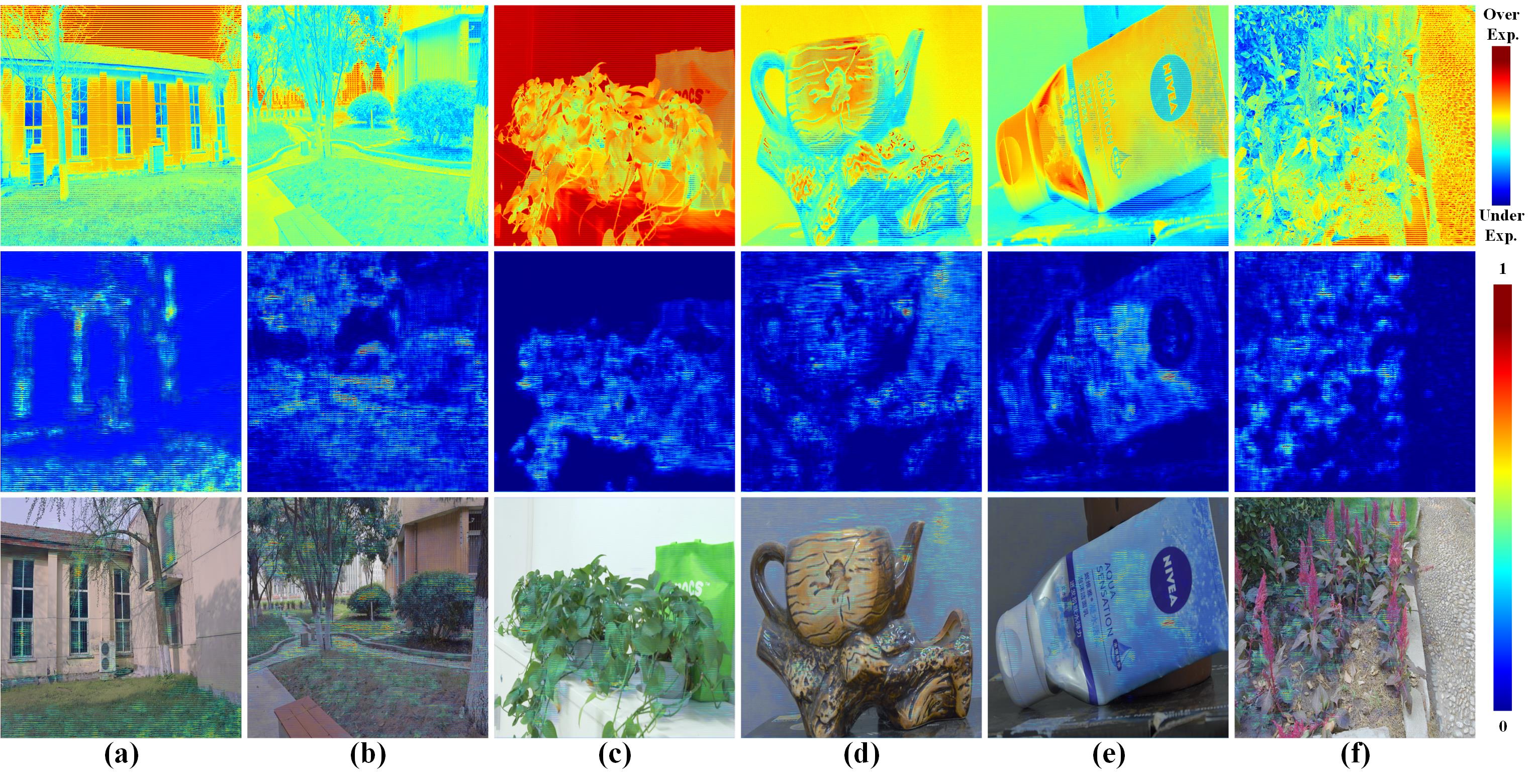
Figure 14: Jet color map. The first row shows the input dual-time Bayer radiance image. The second row shows the the output feature from the last layer of EGB. The third row shows the overlay of the EGB’s feature output and tone-mapped ground truth. The results come from the VETHDR-Nikon test set.

The EGB’s output is also visualized. Sixty-four output feature maps are clustered into one feature map through principal component analysis (PCA). Then, the clustered feature map is normalized into 0 to 1 and visulized using a jet color map. as shown in the second row of Fig. 14.

The first row shows the input dual-time Bayer radiance image, where the horizontal stripes are caused by ill exposing. The third row demonstrates the overlay of the EGB’s output and tone-mapped ground truth. The EGB’s features are concentrated on the well-exposed areas. For the ill-exposed areas, e.g., the sky in column (a) and the building in the distance in colomn (b), few activations occur. Therefore, the EGB can focus on extracting features from the well-exposed areas to compensate for the main branch, which avoids the effect of saturation noise caused by ill exposing.

More visualization examples are shown in the last column of Fig. 12. All the other methods lead to unnatural color distortions. On the contrary, the compensation information from the EGB enables accurate HDR restoration. This result proves that the compensation information can effectively improve the imaging quality of the RB.

IV-D Ablation Study

Experiments on different models are conducted to validate the necessity of each part in our proposed framework. We use an RB with 16 blocks as the baseline and compare 3 models with it. When the SVC is not used, it is replaced with Opt-base. The first one has SVC in the network without EGB. The second one has EGB in the network without SVC. The third one is our proposed complete model, which has two SVCs and one EGB, the SVC is in front of the RB and EGB respectively.

TABLE VII: Quantitative comparison of models with different components. The best results are shown in bold, and the second-best results are shown in blue. The results come from the VETHDR-Nikon test set.

Method	HDR-MAE	HDR-MSE	HDR-VDP	HDR-PSNR-RGB	HDR-SSIM-RGB	HDR-PSNR-Y	HDR-SSIM-Y	P [$10^{6}$]	FLOPs [$10^{11}$]
RB	2.982	53.874	65.59	41.38	0.9786	43.99	0.9860	1.221	2.813
RB+SVC	2.881	40.052	65.69	41.91	0.9791	44.33	0.9861	1.234	2.816
RB+EGB	2.861	47.835	65.83	41.72	0.9794	44.32	0.9865	1.850	4.263
RB+2xSVC+EGB	2.777	38.713	66.02	42.15	0.9797	44.56	0.9865	1.912	4.352

TABLE VIII: Quantitative comparison of models with different components. The best results are shown in bold, and the second-best results are shown in blue. The results come from the VETHDR-Canon test set.

Method	HDR-MAE	HDR-MSE	HDR-VDP	HDR-PSNR-RGB	HDR-SSIM-RGB	HDR-PSNR-Y	HDR-SSIM-Y	P [$10^{6}$]	FLOPs [$10^{11}$]
RB	2.290	26.957	70.41	42.01	0.9889	43.70	0.9922	1.221	2.813
RB+SVC	2.280	25.408	70.43	42.20	0.9890	43.75	0.9921	1.234	2.816
RB+EGB	2.151	24.382	70.67	42.47	0.9895	44.06	0.9925	1.850	4.263
RB+2xSVC+EGB	2.146	23.572	70.64	42.57	0.9897	44.12	0.9926	1.912	4.352

The test results are shown in Table VII and Table VIII. They present that RB+SVC and RB+EGB have significant improvements concerning the RB from the 7 evaluation metrics points of view, which demonstrates the effectiveness of the proposed SVC and EGB. In terms of the complete model, RB+2xSVC+EGB surpasses others in image quality.

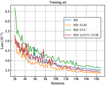
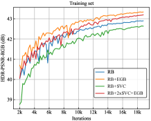
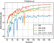
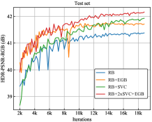
Figure 15: The training plot on the training set, validation set, and test set. The results come from the VETHDR-Nikon test set.

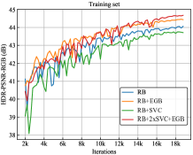
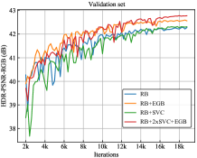
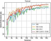
Figure 16: The training plot on the training set, validation set, and test set. The results come from the VETHDR-Canon dataset.

In order to verify the effectiveness of SVC and EGB more comprehensively, the training plots of RB, RB+SVC, RB+EGB, and RB+2xSVC+EGB are shown in Fig. 15 and Fig. 16. We can see that though RB has better convergence on training sets, it is not as robust as RB+SVC and RB+EGB on validation and test sets. Thus, both SVC and EGB improve the generalization ability of CNN. In addition, RB+2xSVC+EGB performs the best across both validation and test sets.

IV-E Speed Evaluation

TABLE IX: The FLOPs and running time required to process images at different resolutions with RB+2xSVC+EGB.

Input Resolution	FLOPs [$10^{11}$]	Time(ms)
$120\times 120$	0.272	17.943
$240\times 240$	1.088	71.772
$360\times 360$	2.448	161.486
$480\times 480$	4.352	287.086
$600\times 600$	6.800	448.573
$720\times 720$	9.793	645.945
$840\times 840$	13.329	879.202
$960\times 960$	17.409	1148.346

In order to evaluate the running speed of our complete model RB+2xSVC+EGB when dealing with different resolutions, Table IX lists the test results of the RB+2xSVC+EGB on GTX 1080Ti. Note that the running time of this model are proportional to the FLOPs and image resolution.

IV-F Comparison with Existing Algorithms

TABLE X: Quantitative comparison between existing methods and our complete model. The best results are shown in bold, and the second-best results are shown in blue. The results come from the VETHDR-Nikon test set.

Method	HDR-MAE	HDR-MSE	HDR-VDP	HDR-PSNR-RGB	HDR-SSIM-RGB	HDR-PSNR-Y	HDR-SSIM-Y	P [$10^{6}$]	FLOPs [$10^{11}$]
Gharbi et al. [24]	3.699	56.522	64.47	39.79	0.9703	42.06	0.9794	0.561	0.330
Xu et al. [26]	3.191	48.28	65.31	40.89	0.9759	43.31	0.9841	1.021	0.467
An et al. [13]	4.167	71.635	61.64	38.95	0.9659	41.43	0.9776	9.480	4.616
An et al. [44]	6.050	92.197	63.84	37.20	0.9676	38.95	0.9781	53.631	13.196
Akyuz et al. [18]	3.414	61.856	61.90	39.79	0.9692	42.46	0.9803	1.553	3.579
Suda et al. [19]	6.707	334.793	56.60	34.83	0.9428	37.84	0.9596	—-	—-
Hajisharif et al. [43]	23.745	1446.367	56.58	25.93	0.8305	27.24	0.8584	—-	—-
Serrano et al. [42]	49.531	4041.573	56.70	22.99	0.9239	23.59	0.9326	—-	—-
Xu et al. [53]	2.855	40.88	65.81	41.89	0.9790	44.32	0.9861	2.073	4.773
Ours	2.777	38.713	66.02	42.15	0.9797	44.56	0.9865	1.912	4.352

TABLE XI: Quantitative comparison between existing methods and our complete model. The best results are shown in bold, and the second-best results are shown in blue. The results come from the VETHDR-Canon test set.

Method	HDR-MAE	HDR-MSE	HDR-VDP	HDR-PSNR-RGB	HDR-SSIM-RGB	HDR-PSNR-Y	HDR-SSIM-Y	P [$10^{6}$]	FLOPs [$10^{11}$]
Gharbi et al. [24]	2.529	36.102	69.77	40.81	0.9864	42.04	0.9899	0.561	0.330
Xu et al. [26]	2.310	28.142	70.37	41.83	0.9886	43.31	0.9918	1.021	0.467
An et al. [13]	3.774	60.669	57.79	38.10	0.9744	39.80	0.9813	9.480	4.616
An et al. [44]	5.547	59.729	69.31	37.76	0.9856	38.30	0.9893	53.631	13.196
Akyuz et al. [18]	3.353	58.502	57.78	38.35	0.9754	40.27	0.9823	1.553	3.579
Suda et al. [19]	9.732	269.536	57.27	31.85	0.9392	34.23	0.9481	—-	—-
Hajisharif et al. [43]	10.982	416.847	61.07	29.72	0.8542	31.32	0.8980	—-	—-
Serrano et al. [42]	69.954	7468.299	52.54	19.06	0.8725	19.44	0.8841	—-	—-
Xu et al. [53]	2.366	25.157	70.59	42.23	0.9895	43.78	0.9925	2.073	4.773
Ours	2.146	23.572	70.64	42.57	0.9897	44.12	0.9926	1.912	4.352

The proposed algorithm is compared with seven single-shot HDRI algorithm [13, 44, 18, 19, 43, 42, 53] and two one-stage joint demosaicing algorithms [24, 26] qualitatively and quantitatively on the two datasets. The denoising and super-resolution in [24, 26] are disabled because they are not required by the single-shot dual-time HDRI.

The results about 7 evaluation metrics are reported in Table X and Table XI. With the fouth least number of parameters (P), our method achieves the best performance in HDR-MAE, HDR-MSE, HDR-VDP, HDR-PSNR-RGB, HDR-SSIM-RGB, HDR-PSNR-Y, and HDR-SSIM-Y on the test set. This superiority is mainly benefited from the proposed SVC and EGB for the single-shot HDRI.

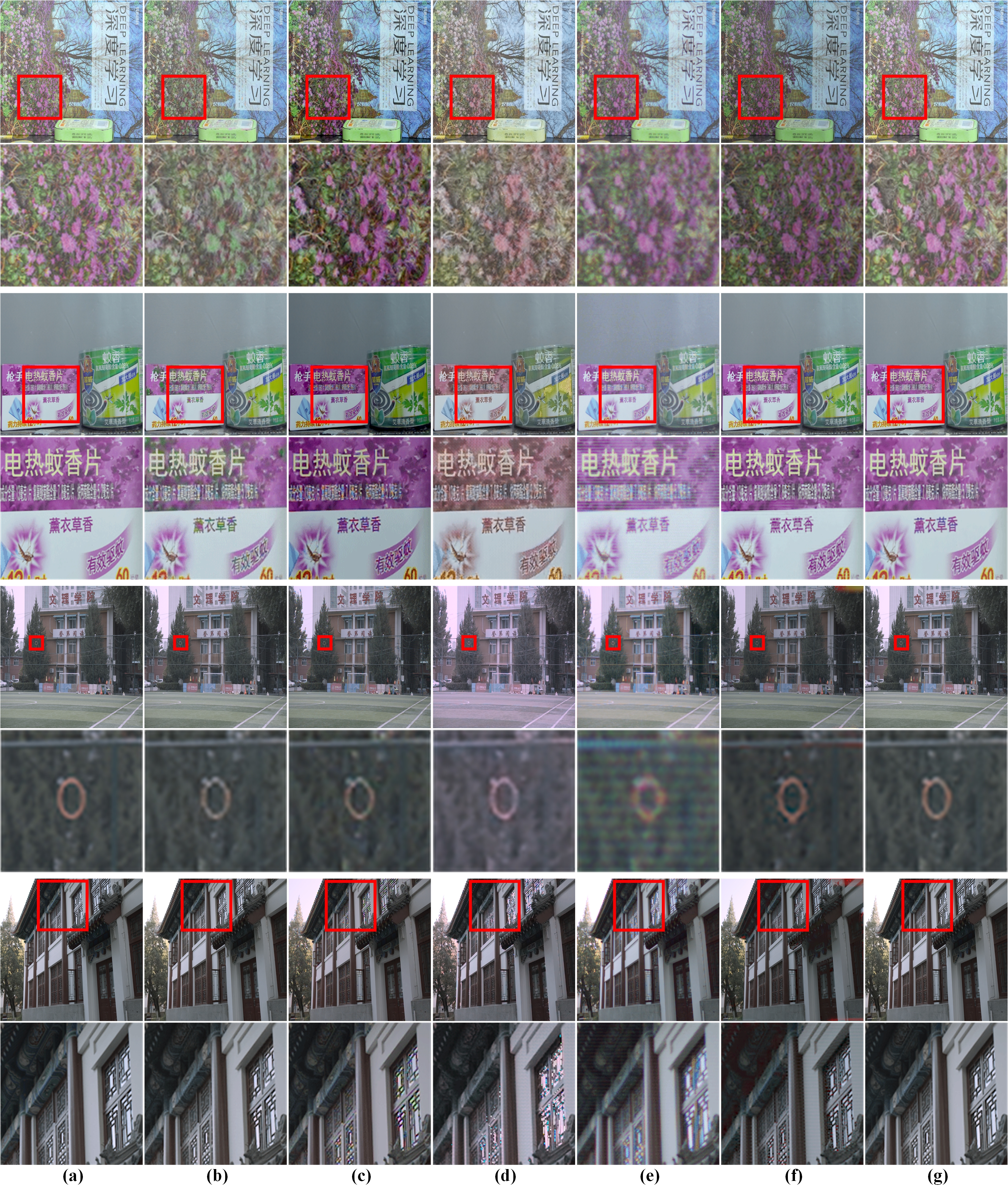
Figure 17: Qualitative comparison between existing methods and our complete model. (a) Ground truth, (b) An et al. [44], (c) Akyuz et al. [18], (d) Suda et al. [19], (e) Hajisharif et al. [43], (f) Serrano et al. [42], (g) Ours. The results come from the VETHDR-Nikon test set and VETHDR-Canon test set.

For a qualitative comparison, the tone-mapping algorithm [64] is applied to compress the generated radiance maps for display. The synthesized results and their detailed parts are shown in Fig. 17. In the first row, the color of flowers is synthesized incorrectly in (b) and (d). The texture of the flower is blurred in (e). The images in (c) and (f) are generally slightly darker than the ground truth. In the second row, the luminance of images in (c) and (e) is different from the ground-truth, and the color of images in (b) and (d) is abnormal. Evident horizontal stripes can also be observed from the results in (e) and (f).

In a nutshell, the results in (e) and (f) are likely to have horizontal stripes, which are caused by the brightness differences in the dual-time Bayer image. The results in (c) tend to have an inappropriate luminance, whereas the results in (b) and (d) have unnatural color. Different from these methods, the proposed algorithm is robust to most scenes, providing accurate HDR restoration. The overall comparison demonstrates the effectiveness of the proposed EGB and SVC.

V Conclusion Remarks and Discussion

In this paper, a novel CNN-based method is proposed to restore high-quality HDR images at full resolution for single-shot HDRI. The proposed CNN includes two distinctive components, the SVC and the exposure-guidance method by which the CNN is more explainable. Experimental results demonstrate that the proposed algorithm outperforms a few existing algorithms. The proposed algorithm focuses on HDR images. The idea of joint demosaicing and HDRI within a single shot can avoid cumulative errors. Since single-shot HDRI has the advantage of not having to take multiple shots, the proposed algorithm can also be extended for HDR videos [22].

Note that the two distinctive components can be extended to other low-level image processing tasks. The SVC can be easily inserted into other networks to process Bayer image with or without SVE, and can be redesigned into flexible variants when the data pattern or SVE changes. The exposure-guidance method can be used to study other HDRI problems, such as [61, 62], allowing CNN to reduce the interference of ill-exposed pixels. It is worth noting that the proposed algorithm can be further improved through the related technologies of augmentation and transfer learning. All these problems will be studied in our future research.

References

- [1] F. Banterle, A. Artusi, K. Debattista, and A. Chalmers, Advanced High Dynamic Range Imaging: Theory and Practice (2nd Edition). Natick, MA, USA: AK Peters (CRC Press), July 2017.
- [2] J. Han, C. Zhou, P. Duan, Y. Tang, C. Xu, C. Xu, T. Huang, and B. Shi, “Neuromorphic camera guided high dynamic range imaging,” in Proceedings of the IEEE/CVF Conference on Computer Vision and Pattern Recognition, 2020, pp. 1730–1739.
- [3] C. LeGendre, W.-C. Ma, R. Pandey, S. Fanello, C. Rhemann, J. Dourgarian, J. Busch, and P. Debevec, “Learning illumination from diverse portraits,” in SIGGRAPH Asia 2020 Technical Communications, 2020, pp. 1–4.
- [4] K. R. Prabhakar, S. Agrawal, D. K. Singh, B. Ashwath, and R. V. Babu, “Towards practical and efficient high-resolution hdr deghosting with cnn,” in Computer Vision–ECCV 2020: 16th European Conference, Glasgow, UK, August 23–28, 2020, Proceedings, Part XXI 16. Springer, 2020, pp. 497–513.
- [5] Q. Wang, W. Chen, X. Wu, and Z. Li, “Detail-enhanced multi-scale exposure fusion in yuv color space,” IEEE Transactions on Circuits and Systems for Video Technology, vol. 30, no. 8, pp. 2418–2429, 2019.
- [6] F. Kou, Z. Li, C. Wen, and W. Chen, “Multi-scale exposure fusion via gradient domain guided image filtering,” in IEEE International Conference on Multimedia and Expo, 2017, pp. 1105–1110.
- [7] Q. T. Wang, W. H. Chen, X. M. Wu, and Z. G. Li, “Detail-enhanced multi-scale exposure fusion in yuv color space,” IEEE Trans. on Circuits and System for Video Technology, vol. 30, no. 8, pp. 2418–2429, 2020.
- [8] J. Cai, S. Gu, and L. Zhang, “Learning a deep single image contrast enhancer from multi-exposure images,” IEEE Transactions on Image Processing, vol. 27, no. 4, pp. 2049–2062, 2018.
- [9] Z. Li, J. Zheng, Z. Zhu, and S. Wu, “Selectively detail-enhanced fusion of differently exposed images with moving objects,” IEEE Trans. on Image Processing, vol. 23, no. 10, pp. 4372–4382, 2014.
- [10] A. Srikantha and D. Sidibé, “Ghost detection and removal for high dynamic range images: Recent advances,” Signal Processing: Image Communication, vol. 27, no. 6, pp. 650–662, 2012.
- [11] O. T. Tursun, A. O. Akyüz, A. Erdem, and E. Erdem, “The state of the art in hdr deghosting: A survey and evaluation,” in Computer Graphics Forum, vol. 34, no. 2. Wiley Online Library, 2015, pp. 683–707.
- [12] J. Zheng, Z. Li, Z. Zhu, S. Wu, and S. Rahardja, “Hybrid patching for a sequence of differently exposed images with moving objects,” IEEE Trans. on Image Processing, vol. 22, no. 12, pp. 5190–5201, 2013.
- [13] V. G. An and C. Lee, “Single-shot high dynamic range imaging via deep convolutional neural network,” in APSIPA ASC, 2017, pp. 1768–1772.
- [14] E. Francois, Y. He, X. Li, A. Luthra, and C. A. Segall, “High dynamic range and wide color gamut video coding in hevc: status and potential future enhancements,” IEEE Trans. on Circuits and System for Video Technology, vol. 26, no. 1, pp. 63–75, 2016.
- [15] Y. Zhang, M. Naccari, D. Agrafiotis, M. Mrak, and R. Bull, “High dynamic range video compression exploiting luminance masking,” IEEE Trans. on Circuits and System for Video Technology, vol. 26, no. 5, pp. 950–964, 2016.
- [16] Z. Wei, C. Y. Wen, and Z. G. Li, “Local inverse tone mapping for scalable high dynamic range image coding,” IEEE Trans. on Circuits and System for Video Technology, vol. 28, no. 2, pp. 550–555, 2018.
- [17] S. K. Nayar and T. Mitsunaga, “High dynamic range imaging: Spatially varying pixel exposures,” in Proceedings IEEE Conference on Computer Vision and Pattern Recognition, vol. 1, 2000, pp. 472–479.
- [18] A. O. Akyüz et al., “Deep joint deinterlacing and denoising for single shot dual-iso hdr reconstruction,” IEEE Transactions on Image Processing, vol. 29, pp. 7511–7524, 2020.
- [19] T. Suda, M. Tanaka, Y. Monno, and M. Okutomi, “Deep snapshot hdr imaging using multi-exposure color filter array,” in Proceedings of the Asian Conference on Computer Vision, 2020.
- [20] J. Gu, Y. Hitomi, T. Mitsunaga, and S. Nayar, “Coded rolling shutter photography: Flexible space-time sampling,” in IEEE International Conference on Computational Photography, 2010, pp. 1–8.
- [21] H. Cho, S. J. Kim, and S. Lee, “Single-shot high dynamic range imaging using coded electronic shutter,” in Computer Graphics Forum, vol. 33, no. 7. Wiley Online Library, 2014, pp. 329–338.
- [22] N. K. Kalantari and R. Ramamoorthi, “Deep hdr video from sequences with alternating exposures,” in Computer Graphics Forum, vol. 38, no. 2. Wiley Online Library, 2019, pp. 193–205.
- [23] Y. Lee, K. Hirakawa, and T. Q. Nguyen, “Joint defogging and demosaicking,” IEEE Trans. on Image Processing, vol. 26, no. 6, pp. 3051–3063, 2016.
- [24] M. Gharbi, G. Chaurasia, S. Paris, and F. Durand, “Deep joint demosaicking and denoising,” ACM Trans. on Graphics, vol. 35, no. 6, pp. 1–12, 2016.
- [25] X. Xu, Y. Ye, and X. Li, “Joint demosaicing and super-resolution (jdsr): Network design and perceptual optimization,” IEEE Trans. on Computational Imaging, 2020.
- [26] X. Xu, Y. Ma, and W. Sun, “Towards real scene super-resolution with raw images,” in Proceedings of the IEEE Conference on Computer Vision and Pattern Recognition, 2019, pp. 1723–1731.
- [27] G. Qian, J. Gu, J. S. Ren, C. Dong, F. Zhao, and J. Lin, “Trinity of pixel enhancement: a joint solution for demosaicking, denoising and super-resolution,” arXiv preprint arXiv:1905.02538, 2019.
- [28] P. E. Debevec and J. Malik, “Recovering high dynamic range radiance maps from photographs,” in Conferenceon Computer Graphics & Interactive Techniques, 1997, pp. 369–378.
- [29] X. Wang, K. Yu, C. Dong, and C. C. Loy, “Recovering realistic texture in image super-resolution by deep spatial feature transform,” in Proceedings of the IEEE conference on computer vision and pattern recognition, 2018, pp. 606–615.
- [30] C. Ma, Y. Rao, Y. Cheng, C. Chen, J. Lu, and J. Zhou, “Structure-preserving super resolution with gradient guidance,” in Proceedings of the IEEE/CVF Conference on Computer Vision and Pattern Recognition, 2020, pp. 7769–7778.
- [31] P. Sen, N. K. Kalantari, M. Yaesoubi, S. Darabi, D. B. Goldman, and E. Shechtman, “Robust patch-based hdr reconstruction of dynamic scenes.” ACM Trans. Graph., vol. 31, no. 6, pp. 203–1, 2012.
- [32] N. D. Bruce, “Expoblend: Information preserving exposure blending based on normalized log-domain entropy,” Computers & Graphics, vol. 39, pp. 12–23, 2014.
- [33] T.-H. Oh, J.-Y. Lee, Y.-W. Tai, and I. S. Kweon, “Robust high dynamic range imaging by rank minimization,” IEEE transactions on pattern analysis and machine intelligence, vol. 37, no. 6, pp. 1219–1232, 2014.
- [34] Y. Niu, J. Wu, W. Liu, W. Guo, and R. W. Lau, “Hdr-gan: Hdr image reconstruction from multi-exposed ldr images with large motions,” IEEE Transactions on Image Processing, vol. 30, pp. 3885–3896, 2021.
- [35] T. Grosch et al., “Fast and robust high dynamic range image generation with camera and object movement,” Vision, Modeling and Visualization, RWTH Aachen, vol. 277284, 2006.
- [36] O. Gallo, A. Troccoli, J. Hu, K. Pulli, and J. Kautz, “Locally non-rigid registration for mobile hdr photography,” in Proceedings of the IEEE Conference on Computer Vision and Pattern Recognition Workshops, 2015, pp. 49–56.
- [37] J. Hu, O. Gallo, K. Pulli, and X. Sun, “Hdr deghosting: How to deal with saturation?” in Proceedings of the IEEE Conference on Computer Vision and Pattern Recognition, 2013, pp. 1163–1170.
- [38] E. Miandji, J. Unger, and C. Guillemot, “Multi-shot single sensor light field camera using a color coded mask,” in 2018 26th European Signal Processing Conference (EUSIPCO). IEEE, 2018, pp. 226–230.
- [39] H. Takeda, S. Farsiu, and P. Milanfar, “Kernel regression for image processing and reconstruction,” IEEE Trans. on Image Processing, vol. 16, no. 2, pp. 349–366, 2007.
- [40] R. Gil Rodríguez and M. Bertalmío, “High quality video in high dynamic range scenes from interlaced dual-iso footage,” in IS&T International Symposium on Electronic Imaging Science and Technology; 2016 Febr. 14-18; San Francisco (CA, USA). Springfield: IS&T; 2016. Digital Photography and Mobile Imaging XII, p. DPMI-245.1 [7 p.]. The Society for Imaging Science and Technology (IS&T), 2016.
- [41] I. Choi, S.-H. Baek, and M. H. Kim, “Reconstructing interlaced high-dynamic-range video using joint learning,” IEEE Trans. on Image Processing, vol. 26, no. 11, pp. 5353–5366, 2017.
- [42] A. Serrano, F. Heide, D. Gutierrez, G. Wetzstein, and B. Masia, “Convolutional sparse coding for high dynamic range imaging,” in Computer Graphics Forum, vol. 35, no. 2. Wiley Online Library, 2016, pp. 153–163.
- [43] S. Hajisharif, J. Kronander, and J. Unger, “Adaptive dualiso hdr reconstruction,” EURASIP Journal on Image and Video Processing, vol. 2015, no. 1, p. 41, 2015.
- [44] A. G. Vien and C. Lee, “Single-shot high dynamic range imaging via multiscale convolutional neural network,” IEEE Access, vol. 9, pp. 70 369–70 381, 2021.
- [45] S. Farsiu, M. Elad, and P. Milanfar, “Multiframe demosaicing and super-resolution of color images,” IEEE Trans. on Image Processing, vol. 15, no. 1, pp. 141–159, 2005.
- [46] R. Ramanath, W. E. Snyder, G. L. Bilbro, and W. A. Sander, “Demosaicking methods for bayer color arrays,” Journal of Electronic imaging, vol. 11, no. 3, pp. 306–315, 2002.
- [47] R. Lukac, K. Martin, and K. N. Plataniotis, “Demosaicked image postprocessing using local color ratios,” IEEE Transactions on Circuits and Systems for Video Technology, vol. 14, no. 6, pp. 914–920, 2004.
- [48] S.-C. Pei and I.-K. Tam, “Effective color interpolation in ccd color filter arrays using signal correlation,” IEEE Transactions on Circuits and Systems for video technology, vol. 13, no. 6, pp. 503–513, 2003.
- [49] X. Chen, L. He, G. Jeon, and J. Jeong, “Multidirectional weighted interpolation and refinement method for bayer pattern cfa demosaicking,” IEEE Transactions on Circuits and Systems for Video Technology, vol. 25, no. 8, pp. 1271–1282, 2014.
- [50] K. Hirakawa and T. W. Parks, “Adaptive homogeneity-directed demosaicing algorithm,” IEEE Trans. on Image Processing, vol. 14, no. 3, pp. 360–369, 2005.
- [51] O. Kapah and H. Z. Hel-Or, “Demosaicking using artificial neural networks,” in Applications of Artificial Neural Networks in Image Processing V, vol. 3962. International Society for Optics and Photonics, 2000, pp. 112–120.
- [52] R. Lukac, K. N. Plataniotis, and D. Hatzinakos, “Color image zooming on the bayer pattern,” IEEE Transactions on Circuits and Systems for Video Technology, vol. 15, no. 11, pp. 1475–1492, 2005.
- [53] Y. Xu, Z. Liu, X. Wu, W. Chen, and Z. Li, “Restoration of hdr images for sve-based hdri via a novel dcnn,” in 2021 IEEE International Conference on Multimedia and Expo (ICME). IEEE, 2021, pp. 1–6.
- [54] R. Lukac, K. N. Plataniotis, D. Hatzinakos, and M. Aleksic, “A novel cost effective demosaicing approach,” IEEE Transactions on Consumer Electronics, vol. 50, no. 1, pp. 256–261, 2004.
- [55] W. Lu and Y.-P. Tan, “Color filter array demosaicking: new method and performance measures,” IEEE transactions on image processing, vol. 12, no. 10, pp. 1194–1210, 2003.
- [56] D. Verma, M. Kumar, and S. Eregala, “Deep demosaicing using resnet-bottleneck architecture,” in International Conference on Computer Vision and Image Processing. Springer, 2019, pp. 170–179.
- [57] C. Ledig, L. Theis, F. Huszár, J. Caballero, A. Cunningham, A. Acosta, A. Aitken, A. Tejani, J. Totz, Z. Wang et al., “Photo-realistic single image super-resolution using a generative adversarial network,” in Proceedings of the IEEE conference on computer vision and pattern recognition, 2017, pp. 4681–4690.
- [58] H. Ren, M. El-Khamy, and J. Lee, “Dn-resnet: Efficient deep residual network for image denoising,” in Asian Conference on Computer Vision. Springer, 2018, pp. 215–230.
- [59] H. Zhao, O. Gallo, I. Frosio, and J. Kautz, “Loss functions for image restoration with neural networks,” IEEE Trans. on Computational Imaging, vol. 3, no. 1, pp. 47–57, 2016.
- [60] D. Marnerides, T. Bashford-Rogers, J. Hatchett, and K. Debattista, “Expandnet: A deep convolutional neural network for high dynamic range expansion from low dynamic range content,” in Computer Graphics Forum, vol. 37, no. 2. Wiley Online Library, 2018, pp. 37–49.
- [61] C. Zheng, Z. Li, Y. Yang, and S. Wu, “Exposure interpolation via hybrid learning,” in IEEE International Conference on Acoustics, Speech and Signal Processing, 2020, pp. 2098–2102.
- [62] C. B. Zheng, Z. G. Li, Y. Yang, and S. Q. Wu, “Single image brightening via multi-scale exposure fusion with hybrid learning,” IEEE Transactions on Circuits and Systems for Video Technology, vol. 31, no. 8, pp. 1–10, 2021.
- [63] B. Funt and L. Shi, “The effect of exposure on maxrgb color constancy,” in Human Vision and Electronic Imaging XV, vol. 7527. International Society for Optics and Photonics, 2010, p. 75270Y.
- [64] E. Reinhard, M. Stark, P. Shirley, and J. Ferwerda, “Photographic tone reproduction for digital images,” in Proceedings of the 29th annual conference on Computer graphics and interactive techniques, 2002, pp. 267–276.
- [65] C.-C. Weng, H. Chen, and C.-S. Fuh, “A novel automatic white balance method for digital still cameras,” in 2005 IEEE International Symposium on Circuits and Systems (ISCAS). IEEE, 2005, pp. 3801–3804.
- [66] T. O. Aydın, R. Mantiuk, and H.-P. Seidel, “Extending quality metrics to full luminance range images,” in Human vision and electronic imaging xiii, vol. 6806. International Society for Optics and Photonics, 2008, p. 68060B.
- [67] R. Mantiuk, K. J. Kim, A. G. Rempel, and W. Heidrich, “Hdr-vdp-2: A calibrated visual metric for visibility and quality predictions in all luminance conditions,” ACM Transactions on graphics (TOG), vol. 30, no. 4, pp. 1–14, 2011.
- [68] Z. Wang, A. C. Bovik, H. R. Sheikh, and E. P. Simoncelli, “Image quality assessment: from error visibility to structural similarity,” IEEE Trans. on Image Processing, vol. 13, no. 4, pp. 600–612, 2004.
- [69] W. Shi, J. Caballero, F. Huszár, J. Totz, A. P. Aitken, R. Bishop, D. Rueckert, and Z. Wang, “Real-time single image and video super-resolution using an efficient sub-pixel convolutional neural network,” in Proceedings of the IEEE conference on computer vision and pattern recognition, 2016, pp. 1874–1883.
- [70] M. A. Robertson, S. Borman, and R. L. Stevenson, “Estimation-theoretic approach to dynamic range enhancement using multiple exposures,” Journal of Electronic Imaging, vol. 12, no. 2, pp. 219–228, 2003.