Auxiliary Loss Reweighting for Image Inpainting

Abstract

Image Inpainting is a task that aims to fill in missing regions of corrupted images with plausible contents. Recent inpainting methods have introduced perceptual and style losses as auxiliary losses to guide the learning of inpainting generators. Perceptual and style losses help improve the perceptual quality of inpainted results by supervising deep features of generated regions. However, two challenges have emerged with the usage of auxiliary losses: (i) the time-consuming grid search is required to decide weights for perceptual and style losses to properly perform, and (ii) loss terms with different auxiliary abilities are equally weighted by perceptual and style losses. To meet these two challenges, we propose a novel framework that independently weights auxiliary loss terms and adaptively adjusts their weights within a single training process, without a time-consuming grid search. Specifically, to release the auxiliary potential of perceptual and style losses, we propose two auxiliary losses, Tunable Perceptual Loss (TPL) and Tunable Style Loss (TSL) by using different tunable weights to consider the contributions of different loss terms. TPL and TSL are supersets of perceptual and style losses and release the auxiliary potential of standard perceptual and style losses. We further propose the Auxiliary Weights Adaptation (AWA) algorithm, which efficiently reweights TPL and TSL in a single training process. AWA is based on the principle that the best auxiliary weights would lead to the most improvement in inpainting performance. We conduct experiments on publically available datasets and find that our framework helps current SOTA methods achieve better results.

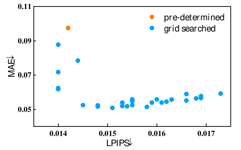
(a)

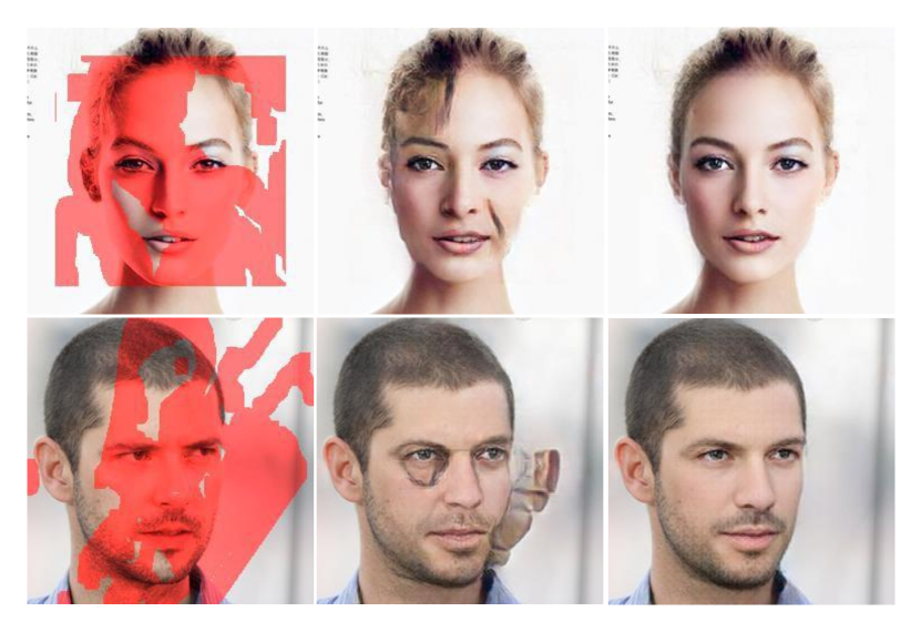
(b)

Figure 1: (a) Inpainting performances of RFR [1] model trained with differently weighted perceptual and style losses on CelebA-HQ [2] dataset, and inpainting performance is sensitive to auxiliary weights. Blue dots represent models trained with grid searched auxiliary weights, and the orange dot is the model trained following default settings. ^↓ means lower is better. (b) Visual results of default model and grid searched model. From left to right: masked images, default results and grid searched results. Better results can be found through grid search.

I Introduction

Image inpainting is an image restoration task that aims to fill in corrupted image regions with visually-plausible contents coherent with untainted regions. Image inpainting is widely adopted in real-world applications, such as face editing [3] , object removal [4], photo restoration etc. The challenge of the inpainting task is to generate patches with limited information from known regions.

Early image inpainting methods [5, 6, 7] restore missing regions by searching best patches based on hand-crafted features or propagation, which perform well when dealing with images with modest corruptions. Benefit from the development of deep neural networks, recent learning-based image inpainting methods [8, 9, 10, 1, 11] employed deep Convolutional Neural Networks (CNNs) to build generators that model distant relationships and generate high-quality patches for images with large holes, and the generators are guided by per-pixel reconstruction loss and adversarial loss [12]. Many current image inpainting methods [13, 14, 11] also introduced perceptual loss [15] and style loss [16] as auxiliary losses to further improve the perceptual quality of inpainting results. Standard perceptual or style loss is defined as the summation of several loss terms. Loss terms are based on different deep features of generated and ground truth images, where the deep features are extracted by pre-trained VGG network [17]. Different from reconstruction or adversarial loss which directly supervise the generated images, the auxiliary losses supervise deep features of generated images which indirectly improves the inpainting performance.

Though perceptual and style losses improve inpainting performance, they face several practical challenges. Firstly, extensive hyperparameter tuning and time-consuming cross-validation are required to determine proper weights for auxiliary weights losses to be properly performed, and the training cost grows exponentially with the number of auxiliary weights (see figure 1). Secondly, their functional form restricts auxiliary potentials of deep features: They simply sum several loss terms up and output one coherent loss which equally treats different loss terms, while more useful terms should be emphasized. These challenges motivate us to study the auxiliary loss reweighting algorithm which and release the full potential of feature-based auxiliary losses.

In this paper, we propose a novel framework to release the auxiliary potential of perceptual loss and style loss and eliminate hyperparameter tuning. We first propose TPL and TSL to enable an independent weighting paradigm. TPL and TSL use a group of trainable weights to consider contributions of different loss terms of perceptual and style losses, viewing each loss term as a separate auxiliary loss. They model a family of auxiliary losses for image inpainting which provides a large search space for the grid search. Then, to efficiently determine the proper weights for TPL and TSL, we propose AWA algorithm which dynamically adjusts weights of TPL and TSL and achieves competitive inpainting results in a single training process. AWA achieves this by providing an explicit optimization goal for auxiliary weights: maximizing the inpainting performance after several iterations of training steps. The optimization goal is based on the principle that the best weighted auxiliary losses would lead to the most pleasing inpainting performance.

Experiments on four publicly available datasets demonstrate that best image inpainting performance can be achieved by our framework compared with other image inpainting methods. We further show that AWA algorithm is compatible with current inpainting methods and is better than other loss reweighting competitors. Our paper has the following three contributions:

• We propose AWA algorithm which automatically adjusts auxiliary weights. As far as we know, it is the first time that hyperparameter learning mechanism is introduced to image inpainting.

• We also propose TPL and TSL which model a large family of auxiliary losses and increase the effectiveness of standard perceptual loss and style loss.

• Experiments on four publicly available datasets demonstrate the superiority and universality of our framework.

The rest of the paper is organized as follows. Section II summarizes the related works on image inpainting and loss weights adaptation methods. Section III illustrates our framework, including the form of TPL and TSL losses and the AWA algorithm. In section IV, we discuss the experimental settings. Section V shows the experimental results. In the last section, we conclude the paper and propose future work.

II Related Work

II-A Image Inpainting

The image inpainting approaches are mainly branched into the following groups: patch-based image inpainting [5, 18, 6], diffusion-based image inpainting [19, 20, 21, 22, 23, 7], and learning-based image inpainting [8, 10, 9, 24, 25, 26, 27, 28, 1, 29, 30, 13, 31, 32, 33, 34, 35, 36, 14].

Patch-based methods synthesize the unknown regions by the most identical matched patches in a known area. An influential patch-based inpainting approach was developed by Barnes et al. [5]. Diffusion-based methods fill in tiny missing regions by propagation to diffuse information from the outside to the inside of the hole region. Some other methods [37, 38] combine diffusion-based and patch-based techniques to generate better results. However, these methods have limited performance when dealing with large holes, as they only consider low-level features of the background.

Learning-based methods could generate deterministic high-quality results with low distortion. They use CNN to extract high-level features and model long-distance relationships between the missing and known region. Some methods [24, 9, 13, 39, 33] design specific convolution layers for image inpainting . Some try to use structure information (contour [34], canny edge [25], gradient map [40], segmentation map [31, 32, 28]) to assist inpainting process. Some other methods [27, 41, 8, 42, 30, 29] introduce adversarial loss to increase and diversity of generated results.

Auxiliary losses (e.g. perceptual loss [15] and style losses [24]) are further introduced to increase perceptual quality. Based on deep features, the perceptual loss is used in style transfer learning [15] and was firstly introduced by [24] to handle image inpainting. Style loss is used to ameliorate the periodic unreal patterns brought by perceptual loss. Perceptual and style losses are different from MAE or adversarial losses, as they measure the difference between deep features of generated and ground truth images. Though the perceptual and style losses improve inpainting performance, their functional form restricts auxiliary abilities of deep features, as loss terms are equally treated by simply summing several loss terms up. In this paper, we attempt to independently weight loss terms and dynamically adjust their weights.

II-B Loss Reweighting Algorithms

The correlated work to ours are loss reweighting algorithms that adjust loss weights to achieve balance among multiple loss functions.

In the context of Multi-task learning (MTL), models are trained to give high performance on several different tasks [43, 44, 45]. If several related tasks could assist each other by sharing certain parameters [46, 47], better generalization can be achieved [48, 49]. To achieve better generalization, MTL methods employ loss reweighting algorithms to balance multiple losses. Sener et al.  [47] adjusts the combination among tasks by minimizing the upper bound of the multiple-gradient descent algorithm (MGDA-UB). Chen et al.  [50] adapts task weights by manually restricting gradient norms of different tasks on a common scale to learn tasks at the same pace. At the same time, Kendall et al.  [51] proposed a principled approach that adjusts weights according to uncertainty of tasks. To achieve a better trade-off between accuracy and computational cost of anytime neural networks (ANN) [52], Hu et al.  [53] makes the weights are inversely proportional to the average of each loss.

Closely related to MTL, a good balance between main and auxiliary losses need to be achieved in auxiliary learning (AL) where main and auxiliary losses are jointly optimized, but only the main task’s performance is important. To better use auxiliary losses, in [54] an auxiliary loss is filtered out when it has an opposite gradient direction to the main loss. Some other algorithms have been designed to adjust auxiliary weights by estimating noisy gradient similarity (e.g. inner product [55] and the l2 distance [56]) between main and auxiliary losses. Different from these works, we provide the stable and explicit optimization goal for auxiliary weights.

It is noteworthy that, the proposed AWA is different from current adaptive auxiliary loss techniques [53, 54, 50] which implicitly adjust auxiliary weights by considering loss magnitudes or noisy gradient similarities among main loss and auxiliary losses. The AWA provides an explicit optimization goal for auxiliary weights and increases the inpainting performance.

III Approach

In this section, we first define the notation and the inpainting problem and describe details of TPL and TSL, then we propose our AWA algorithm to dynamically reweight them by setting an explicit optimization goal for weights of TPL and TSL.

III-A Notations and Definitions

Let $\{(\mathbf{x}_{i},\mathbf{y}_{i})\}_{i}$ be the training dataset for image inpainting, where $\mathbf{x}_{i}$ and $\mathbf{y}_{i}$ are the corrupted image and ground truth image, respectively. Current inpainting methods try to learn parameterized generators $g(\cdot;\theta)$ to approximate the function which maps destroyed images to corresponding ground truth. Specifically, after receiving a corrupted image $\mathbf{x}_{i}$, the generator predicts the corresponding ground truth $\tilde{\mathbf{y}}_{i}=g(\mathbf{x}_{i};\theta)$.

The inpainting loss can be defined as the summation of a coherent main loss and an auxiliary loss:

$$\mathcal{L}_{t}(\theta,\phi)=\lambda_{m}\cdot L_{m}(\theta)+\lambda_{a}\cdot L_{a}(\theta),$$ (1)

$$L_{m}(\theta)=(\mathcal{L}_{l1}(\theta),\mathcal{L}_{adv}(\theta),\mathcal{L}_{tv}(\theta))^{T},$$

$$L_{a}(\theta)=(\mathcal{L}_{perc}(\theta),\mathcal{L}_{styl}(\theta))^{T},$$

where the main loss is the dot product of loss vector $L_{m}$ and weight vector $\lambda_{m}$. $L_{m}$ is comprised of the $l_{1}$, adversarial and total variance losses. The coherent auxiliary loss is comprised of perceptual and style losses and weight vector $\lambda_{a}$. The forms of perceptual loss $\mathcal{L}_{perc}$ and style loss $\mathcal{L}_{styl}$ are as follows:

$$\mathcal{L}_{perc}(\theta)=\sum_{n}\mathcal{L}_{perc}^{n}(\theta),\qquad\qquad$$ (2)

$$\mathcal{L}_{perc}^{n}(\theta)=\sum_{i}||\bm{\psi}_{n}(\tilde{\mathbf{y}}_{i})-\bm{\psi}_{n}(\mathbf{y}_{i})||_{1},$$

$$\mathcal{L}_{styl}(\theta)=\sum_{n}\mathcal{L}_{styl}^{n}(\theta),$$ (3)

$$\mathcal{L}_{styl}^{n}(\theta)=\sum_{i}||G(\bm{\psi}_{n}(\tilde{\mathbf{y}}_{i}))-G(\bm{\psi}_{n}(\mathbf{y}_{i}))||_{1},$$

where $\bm{\psi}$ denotes pretrained VGG parameters, and $\bm{\psi}_{n}(.)$ outputs the feature map of the $n$-th chosen layer of the VGG network. As shown in Eq. 2, perceptual loss measures the difference between deep features of generated and ground truth images. Style loss has a similar form, except that it measures the Gram matrices. In Eq. 3 $G(.)$ outputs the Gram matrix of the input deep feature.

III-B Tunable Perceptual and Style Losses

Perceptual and style losses have been introduced by current image inpainting methods [24, 25, 26, 13, 1, 11] to improve the perceptual quality. As mentioned above, they add several loss terms up and use the same weight considering the contribution of different loss terms. However, it restricts the auxiliary potential of deep features, as more useful terms should be emphasized.

To release the potential of deep feature based auxiliary losses, we propose tunable perceptual and style losses (TPL & TSL) which use a group of continuous-valued weights to independently consider contributions of loss terms of perceptual and style losses. In effect, the TPL takes the following form:

$$\mathcal{L}_{tperc}(\theta)=\omega_{p}(\phi_{p})\cdot L_{p}(\theta),$$ (4)

$$L_{p}(\theta)=(\mathcal{L}_{perc}^{1}(\theta),...,\mathcal{L}_{perc}^{N}(\theta))^{T},$$

$$\omega_{p}(\phi_{p})=\lambda_{p}\odot\delta(\phi_{p}).$$

As shown in Eq. LABEL:eq:tunable_perceptual_loss, TPL is the weighted sum of N perceptual loss terms $L_{p}$. The weight vector $\omega_{p}(\phi_{p})$ is the function of continuous-valued parameters $\phi_{p}$. $\psi_{p}$ is activated by sigmoid $\delta(.)$ and element-wise rescaled by $\lambda_{p}$ such that the value range of weights of TPL is from 0 to $\lambda_{p}$, where $\odot$ represents the Hadamard product. Note that TPL is a superset of perceptual loss, and in experiments, all elements of $\psi_{p}$ are equally initialized such that TPL equals perceptual loss to make fair comparisons. Following TPL, we propose TSL to model a family of style loss by adding $\phi_{s}$ to standard style loss, and TSL is defined as follows:

$$\mathcal{L}_{tstyl}(\theta)=\omega_{s}(\phi_{p})\cdot L_{s}(\theta),$$ (5)

$$L_{s}(\theta)=(\mathcal{L}_{styl}^{1}(\theta),...,\mathcal{L}_{styl}^{N}(\theta))^{T},$$

$$\omega_{s}(\phi_{p})=\lambda_{s}\odot\delta(\phi_{s}).$$

where the sigmoid is also applied on $\phi_{s}$, and $\lambda_{s}$ denotes the maximum value of weights of TSL. To simplify notations, we use $\omega_{p}$ and $\omega_{s}$ to represent $\omega_{p}(\phi_{p})$ and $\omega_{s}(\phi_{s})$ respectively. Then the perceptual and style losses can be replaced with TPL and TSL, and the new inpainting loss is defined as follows:

$$\mathcal{L}_{t}(\theta)= \lambda_{m}\cdot L_{m}(\theta)+\omega_{p}\cdot L_{p}(\theta)+\omega_{s}\cdot L_{s}(\theta).$$ (6)

III-C Auxiliary Weights Adaptation

As mentioned above, the TPL and TSL model a larger family of auxiliary loss for image inpainting. However, it is impractical to use grid search to determine proper weights for TPL and TSL, as it takes days to train a single inpainting model with one combination of auxiliary weights. To properly reweight auxiliary losses, we propose AWA algorithm which alters between optimizing model parameters ($\theta$) and adaptively adjusting auxiliary parameters ($\phi_{p}$ and $\phi_{s}$) in a single training process.

Auxiliary parameters are learned by optimizing the optimizing goal: maximizing the inpainting performance measured by some metric (e.g. LPIPS) after the model trained by the TPL and TSL for $K$ steps. Formally, objective of auxiliary parameters $\phi_{p}$ and $\phi_{s}$ is as follows:

$$\phi_{p}^{*},\phi_{s}^{*}= \mathop{argmin}_{\phi_{p},\phi_{s}}\mathcal{L}_{c}(\theta^{K}),$$ (7)

$$s.t.\ \theta^{K}= \theta-\alpha\sum_{j=1}^{K}(\lambda_{m}^{T}J_{m}(\theta^{j})+\omega_{p}^{T}J_{p}(\theta^{j})$$

$$+\omega_{s}^{T}J_{s}(\theta^{j})),$$

where the metric is defined as $\mathcal{L}_{c}(\theta^{K})=\sum_{i}l_{c}(\mathbf{x}_{i},\mathbf{y}_{i},\theta^{K})$. $\theta^{K}$ denotes the model parameter updated $K$ steps from $\theta$, and $\alpha$ is the model learning rate. $J_{m}(\theta^{j})$, $J_{p}(\theta^{j})$ and $J_{s}(\theta^{j})$ are Jacobian matrices of vector loss $L_{m}$, $L_{p}$ and $L_{s}$ with respect to generator parameter at $j$-th step (In Adam [57] these matrices are also rescaled element-wise).

Though we can directly optimize auxiliary parameters on $\mathcal{L}_{c}$ through a gradient-based process, it requires to save $K$ steps of computational graph and differentiating through the optimization process over $\theta$. In practice, we solve this by proposing the surrogate loss function $\mathcal{L}_{sg}(\phi_{p},\phi_{s})$, which takes the following form:

$$\mathcal{L}_{sg}(\phi_{p},\phi_{s})= -\nabla_{\theta}^{T}\mathcal{L}_{c}(\theta^{K})\sum_{j}(J_{p}^{T}(\theta^{j})\omega_{p}$$ (8)

$$+J_{s}^{T}(\theta^{j})\omega_{s}).$$

The surrogate loss is comprised of Jacobian matrices of auxiliary losses and the gradient of $\mathcal{L}_{c}$ at point $\theta^{K}$ without differentiating through K step updates of model parameters. Please refer to the Appendix for the derivation of Eq. 8.

After the update of auxiliary parameters, model parameters $\theta$ could be learned by newly weighted auxiliary losses using the loss function in Eq. 6. Our algorithm is summarized in Algorithm.1. We show a gradient descent version of AWA for simplicity, and parameters can also be optimized by other optimizers such as Adam. In practice, we use LPIPS as the guiding metrics, as the ablative studies show that LPIPS is more fit for AWA, please refer to section V-B for more details.

Algorithm 1 Adaptive Auxiliary Loss.

Pre-determined hyperparameter $K$, $\lambda_{p}$ and $\lambda_{s}$. Randomly initialized auxiliary parameters $\phi_{p}$ and $\phi_{s}$ and the learning rate $\beta$. Randomly initialized model parameters $\theta$ and the corresponding learning rate $\alpha$.

while $\theta\ not\ converged$ do

     Compute $\theta^{K}$: $\theta^{K}=\theta-\alpha\sum_{j=1}^{K}(\lambda_{m}^{T}J_{m}(\theta^{j})+\omega_{p}^{T}J_{p}(\theta^{j})$

                            $+\omega_{s}^{T}J_{s}(\theta^{j}))$

     Save Jacobian matrices:

     $\{J_{p}(\theta^{1}),...,J_{p}(\theta^{K}),J_{s}(\theta^{1}),...,J_{s}(\theta^{K})\}$

     Train auxiliary parameters with loss function Eq. 8:

     $\phi_{p}\leftarrow\phi_{p}-\beta\nabla_{\phi_{p}}\mathcal{L}_{sg}(\phi_{p},\phi_{s})$

     $\phi_{s}\leftarrow\phi_{s}-\beta\nabla_{\phi_{s}}\mathcal{L}_{sg}(\phi_{p},\phi_{s})$

     Train $\theta$ with reweighted TPL and TSL with Eq. 6:

     $\theta\leftarrow\theta-\alpha(J_{m}(\theta^{j})\lambda_{m}+J_{p}(\theta^{j})\omega_{p}+J_{s}(\theta^{j})\omega_{s}))$

end while

IV Experimental Settings

IV-A Dataset

We conduct experiments on four commonly used datasets in experiments, namely CelebA [2], CelebA-HQ, Paris-StreetView [58] and Places2 [59]. Besides, an external mask dataset from [24] is also used to produce corrupted images.

• CelebA: Celeba contains more than 200,000 face images, include 162770 training images, 19867 validation images and 19962 testing images, we randomly select 10,000 images from test dataset for testing.

• CelebA-HQ: CelebA-HQ is a dataset that has 30,000 high-resolution face images selected from the CelebA dataset, include 28000 training images and 2000 testing images. All images are resized to $256\times 256$ in our experiments.

• Paris StreetView: Paris StreetView contains 15,000 outdoor building images, with 14900 images for training and 100 images for testing.

• Places2: Places2 is a collection 365 categories scene images which contains 1803640 training images, and we randomly select 10000 images in the test dataset for testing.

• Masks: We use irregular mask dataset provided by [24], in which masks are split into groups according to the relative masked ratio: (0.01,0.1], (0.1,0.2], (0.3,0.4], (0.4,0.5], (0.5,0.6]. Each group has 2000 images.

The size of the training image is 256 × 256. For CelebA, the raw images have a size of 178 × 218, and we crop the 178 x 178 region at the center and resize it to 256 x 256 as the input image. For Paris StreetView and Places2, resizing operation is only needed, as images are squre.

IV-B Inpainting Methods

Our framework is compatible with current CNN based inpainting methods, and in this paper, we apply our framework to train the following inpainting models.

• EG[25] EG uses a two-stage model where the first generator completes edge maps and image generator uses these maps as structure priors to generate images.

• PRVS[26] PRVS devises a network which progressively reconstructs strucure maps as well as visual features.

• CTSDG[11] CTSDG designs a two-stream network which utilizes texture and structure reconstruction to guide the training of encoder and decoder respectively.

IV-C Implementation Details

Our framework are applied to train various SOTA methods [11, 25, 26]. All experiments are implemented by Python on Ubuntu 20.04 system with 2 GeForce RTX 3090 GPUs. With AWA, models are trained following the settings of the SOTA methods. The auxiliary parameters are updated by the AdamW optimizer with $\beta_{1}=0.5$ and $\beta_{2}=0.999$, and the learning rate $\beta$ is $1e^{-3}$. The hyperparameter $K$ is set to 1. For TPL and TSL, $\lambda_{p}$ and $\lambda_{s}$ are set to 2 and 750 respectively. Analogous to [11], the deep features of TPL and TSL are extracted by deep features are from the first three max-pooling layers of the pre-trained VGG-16 network. Our source code is available at https://github.com/HuiSiqi/Auxiliary-Loss-Reweighting-for-Image-Inpainting.

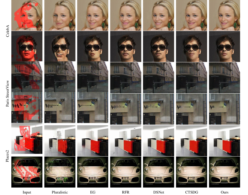
Figure 2: Qualitative comparisons of our results and other image inpainting methods on CelebA, Paris StreetView and Places2. Here, we apply our framework to train CTSDG and generate our results.

TABLE I: Quantitative Comparisons of Our Results and Other Inpainting Methods. The Best Results Are Boldfaced. ^↑ Means Higher Is Better. ^↓ Means Lower Is Better.

DataSet	Metrics	Mask	PIC	EG	PRVS	RFR	DSNet	CTSDG	Ours
CelebA	PSNR ↑	(0.2,0.3]	25.764	27.691	28.633	29.013	28.778	28.521	29.610
		(0.3,0.4]	23.528	26.368	26.373	26.687	26.439	26.200	27.202
		(0.4,0.5]	21.562	24.402	24.525	24.856	24.565	24.356	25.261
		(0.5,0.6]	18.457	21.398	21.750	22.057	21.776	21.610	22.294
	SSIM ↑	(0.2,0.3]	0.8984	0.9328	0.9417	0.9456	0.9433	0.9414	0.9518
		(0.3,0.4]	0.8568	0.9126	0.9113	0.9159	0.9124	0.9090	0.9240
		(0.4,0.5]	0.8078	0.8760	0.8767	0.8825	0.8772	0.8728	0.8921
		(0.5,0.6]	0.7198	0.8072	0.8148	0.8213	0.8137	0.8093	0.8329
	MAE ↓	(0.2,0.3]	0.0252	0.0136	0.0120	0.0111	0.0114	0.0115	0.0100
		(0.3,0.4]	0.0330	0.0175	0.0179	0.0168	0.0174	0.0177	0.0155
		(0.4,0.5]	0.0431	0.0249	0.0249	0.0234	0.0243	0.0248	0.0220
		(0.5,0.6]	0.0657	0.0404	0.0388	0.0366	0.0381	0.0391	0.0354
	LPIPS ↓	(0.2,0.3]	0.0948	0.0637	0.0678	0.0465	0.0472	0.0659	0.0521
		(0.3,0.4]	0.1326	0.0822	0.1034	0.0710	0.0712	0.1005	0.0799
		(0.4,0.5]	0.1765	0.1156	0.1435	0.0987	0.0987	0.1389	0.1112
		(0.5,0.6]	0.2492	0.1766	0.2138	0.1474	0.1458	0.2044	0.1675
	FID ↓	(0.2,0.3]	5.2152	3.2487	4.4684	3.3639	2.9046	4.7415	2.7465
		(0.3,0.4]	7.5484	5.2663	8.7892	6.4810	5.4184	9.3803	4.6354
		(0.4,0.5]	10.832	8.8076	15.3408	11.038	9.0213	15.638	7.3770
		(0.5,0.6]	17.175	16.396	27.478	19.878	15.877	25.199	13.087
Paris StreetView	PSNR ↑	(0.2,0.3]	25.677	27.929	28.354	28.391	28.256	29.276	29.942
		(0.3,0.4]	23.698	25.817	26.241	26.310	26.158	26.888	27.664
		(0.4,0.5]	21.804	24.149	24.126	24.393	24.300	24.969	25.554
		(0.5,0.6]	18.942	21.747	21.419	21.867	21.763	22.263	22.502
	SSIM ↑	(0.2,0.3]	0.8698	0.9167	0.9233	0.9240	0.9210	0.9346	0.9418
		(0.3,0.4]	0.8180	0.8763	0.8835	0.8852	0.8802	0.8945	0.9059
		(0.4,0.5]	0.7519	0.8271	0.8315	0.8356	0.8302	0.8472	0.8609
		(0.5,0.6]	0.6475	0.7545	0.7446	0.7548	0.7488	0.7648	0.7807
	MAE ↓	(0.2,0.3]	0.0281	0.0155	0.0173	0.0171	0.0174	0.0125	0.0115
		(0.3,0.4]	0.0363	0.0222	0.0235	0.0232	0.0237	0.0189	0.0173
		(0.4,0.5]	0.0481	0.0307	0.0320	0.0312	0.0315	0.0266	0.0248
		(0.5,0.6]	0.0707	0.0444	0.0477	0.0454	0.0455	0.0409	0.0398
	LPIPS ↓	(0.2,0.3]	0.1386	0.0778	0.1133	0.0696	0.0785	0.0697	0.0645
		(0.3,0.4]	0.1855	0.1129	0.1455	0.1006	0.1103	0.1109	0.1036
		(0.4,0.5]	0.2528	0.1608	0.1931	0.1413	0.1528	0.1636	0.1532
		(0.5,0.6]	0.3441	0.2298	0.2750	0.2065	0.2204	0.2471	0.2440
	FID ↓	(0.2,0.3]	71.772	41.273	35.892	31.319	35.758	39.695	30.985
		(0.3,0.4]	86.397	53.215	48.371	40.609	46.183	52.841	39.842
		(0.4,0.5]	101.88	70.144	68.103	55.892	61.823	75.214	53.016
		(0.5,0.6]	117.73	89.791	99.863	73.472	83.765	99.140	76.936
Places2	PSNR ↑	(0.2,0.3]	22.070	24.251	25.526	25.026	25.278	25.550	26.407
		(0.3,0.4]	20.066	22.249	23.347	23.166	23.076	23.271	24.007
		(0.4,0.5]	18.393	20.628	21.607	21.525	21.337	21.506	22.159
		(0.5,0.6]	16.139	18.550	19.270	19.278	19.009	19.127	19.622
	SSIM ↑	(0.2,0.3]	0.8388	0.8866	0.9076	0.8995	0.9033	0.9091	0.9225
		(0.3,0.4]	0.7701	0.8343	0.8602	0.8562	0.8536	0.8593	0.8776
		(0.4,0.5]	0.6940	0.7766	0.8072	0.8041	0.7982	0.8041	0.8266
		(0.5,0.6]	0.5936	0.6945	0.7247	0.7220	0.7096	0.7148	0.7398
	MAE ↓	(0.2,0.3]	0.0325	0.0216	0.0183	0.0185	0.0185	0.0185	0.0154
		(0.3,0.4]	0.0465	0.0315	0.0272	0.0269	0.0277	0.0277	0.0238
		(0.4,0.5]	0.0629	0.0429	0.0375	0.0369	0.0383	0.0383	0.0335
		(0.5,0.6]	0.0903	0.0617	0.0556	0.0546	0.0571	0.0572	0.0519
	LPIPS ↓	(0.2,0.3]	0.1625	0.0941	0.0891	0.0982	0.0804	0.0922	0.0670
		(0.3,0.4]	0.2279	0.1369	0.1369	0.1269	0.1174	0.1443	0.1064
		(0.4,0.5]	0.3001	0.1850	0.1918	0.1665	0.1599	0.2022	0.1532
		(0.5,0.6]	0.3911	0.2601	0.2861	0.2336	0.2362	0.2974	0.2472
	FID ↓	(0.2,0.3]	13.477	5.0693	4.3334	4.2622	3.7142	5.2107	2.6902
		(0.3,0.4]	21.831	8.3719	7.9738	6.0240	5.8944	9.7656	4.7671
		(0.4,0.5]	33.158	13.247	13.580	9.0021	9.0499	16.902	7.9979
		(0.5,0.6]	47.170	21.758	26.355	15.400	15.764	31.865	19.181

V Experiments

In this section, we compare our results with several SOTA inpainting methods, both quantitatively and qualitatively. Then, we conduct ablative experiments to study the effects of TPL and TSL, as well as the guidance metric and the hyperparameter K. In analysis, we study the superiority and the universality of our framework, and we show the weight adaptation processes.

V-A Comparisons with State-of-the-art Methods

To demonstrate the effectiveness of our framework, we train CTSDG [11] with our framework, and compare our results with several state-of-the-art image inpainting methods. The models are: PIC [60](CVPR2019), EG [25] (ICCV2019), RFR [1] (CVPR2020), DSNet [13] (TIP2021) and CTSDG [11] (ICCV2021).

Qualitative Comparisons. Fig. 2 presents our results and results of existing image inpainting methods on CelebA, Paris StreetView and Places2. Pluralistic generates results with distorted structures. EG is limited in inferring object contours such as the jaw or the hood. RFR tends to produce artefacts like ink marks. The DSNet is also limited in producing determined structures, and CTSDG generates over blurred contents. Compared with these methods, our results obtain less structure ambiguity and texture inconsistency in the destroyed regions.

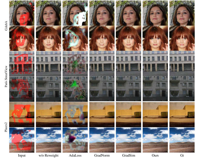
Figure 3: Qualitative comparisons of our algorithm and other three loss reweighting algorithms. w/o Reweight denotes CTSDG trained with fixed auxiliary weights. The middle three lines are results of CTSDG trained with TPL and TSL reweighted by AdaLoss, GradNorm and GradSim respectively. Ours is CTSDG trained with our framework.

Quantitative Comparisons. We also compare their results quantitatively. In this part, we evaluate image inpainting performances in terms of five commonly used metrics: PSNR, SSIM, MAE, LPIPS [61] and FID [62]. Following [61, 13], these metrics can be grouped into two classes of distortion metrics (PSNR, SSIM and MAE) and perception metrics (FID and LPIPS). Distortion metrics are used to quantify the distance between the ground truth image and generated image at the pixel level, while the perception metrics are introduced to measure the high level deep features of generated images. As we find the distortion metrics often contradict human judgements [61], we also use perception metrics to evaluate image qualities from a perspective close to humans.

In TABLE I, we summarize the performance of CTSDG trained by our framework and SOTA methods on datasets of Paris StreetView, CelebA and Places2. What stands out is that our results achieve the best distortion scores, compared with SOTA methods. In particular our framework consistently improves the performance of CTSDG by a large margin across all datasets. As for perception scores, we are better than other SOTA methods except RFR. Though our LPIPS scores are slightly weaker than RFR on CelebA and Paris StreetView, our results have better FID scores. These demonstrates that our framework can efficiently improve performance of current image inpainting method.

TABLE II: Ablative experiments. The best results are $BoldFaced$. ^↑ Means Higher Is Better. ^↓ Means Lower Is better.

Experiment	PSNR ↑	SSIM ↑	MAE ↓	LPIPS ↓	FID ↓
1	32.084	0.9481	0.0128	0.0500	4.9752
2	32.712	0.9535	0.0119	0.0435	5.1987
3	32.909	0.9541	0.0110	0.0403	4.0748
4	32.799	0.9545	0.0111	0.0425	4.5517
5	32.905	0.9535	0.0110	0.0402	4.1045
6	32.880	0.9541	0.0110	0.0404	4.1787

V-B Ablation Study

In this section, we conduct ablative studies of TPL and TSL losses, as well as the guidance metric and the hyperparameter K of AWA. We choose CTSDG as the base model and train generators on CelebA-HQ dataset. Specific settings of the six experiments are as follows:

• Experiment 1: We train CTSDG with standard perceptual and style losses with static auxiliary weights.

• Experiment 2 : We train CTSDG with perceptual and style losses and apply AWA to adapt auxiliary weights. The guidance metric is LPIPS and K is set to 1.

• Experiment 3: We train CTSDG with TPL and TSL and apply AWA to adapt auxiliary weights. The guidance metric is LPIPS and K is set to 1.

• Experiment 4: We replace the guidance metric in Experiment 3 with MAE.

• Experiment 5: We set K in Experiment 3 to 5.

• Experiment 6: We set K in Experiment 3 to 10.

TABLE III: Quantitative Comparisons of Our Algorithm and Other Three Loss Reweighting Algorithms. The Best Results Are Boldfaced. AL, GN and GS denote AdaLoss, GradNorm and GradSim respectively. ^↑ Means Higher Is Better. ^↓ Means Lower Is Better.

Metrics	Mask	Paris StreetView				CelebA				Places2
		AL	GN	GS	Ours	AL	GN	GS	Ours	AL	GN	GS	Ours
PSNR ↑	(0.1,0.2]	23.132	33.730	33.146	33.520	19.695	32.988	32.809	33.073	23.208	30.229	29.685	29.971
	(0.2,0.3]	20.352	30.272	29.639	29.942	15.925	29.458	29.346	29.610	20.432	26.731	26.154	26.407
	(0.3,0.4]	18.707	27.855	27.258	27.664	12.373	26.970	26.937	27.202	18.448	24.349	23.772	24.007
	(0.4,0.5]	16.593	25.792	25.196	25.554	9.417	24.982	24.997	25.261	16.734	22.498	21.935	22.159
	(0.5,0.6]	12.538	22.687	22.339	22.502	7.025	21.898	22.057	22.294	13.874	19.903	19.422	19.622
SSIM ↑	(0.1,0.2]	0.8665	0.9710	0.9678	0.9695	0.8431	0.9749	0.9739	0.9752	0.8869	0.9616	0.9584	0.9605
	(0.2,0.3]	0.7879	0.9452	0.9391	0.9418	0.7534	0.9507	0.9492	0.9518	0.8166	0.9252	0.9187	0.9225
	(0.3,0.4]	0.7242	0.9108	0.9014	0.9059	0.6664	0.9217	0.9200	0.9240	0.7497	0.8823	0.8720	0.8776
	(0.4,0.5]	0.6475	0.8690	0.8549	0.8609	0.5747	0.8885	0.8865	0.8921	0.6793	0.8337	0.8190	0.8266
	(0.5,0.6]	0.5616	0.7941	0.7723	0.7807	0.5150	0.8260	0.8251	0.8329	0.5870	0.7526	0.7296	0.7398
MAE ↓	(0.1,0.2]	0.0244	0.0065	0.0069	0.0067	0.0362	0.0054	0.0055	0.0053	0.0223	0.0079	0.0084	0.0081
	(0.2,0.3]	0.0417	0.0111	0.0118	0.0115	0.0724	0.0103	0.0104	0.0100	0.0391	0.0149	0.0159	0.0154
	(0.3,0.4]	0.0578	0.0168	0.0179	0.0173	0.1277	0.0160	0.0161	0.0155	0.0572	0.0231	0.0246	0.0238
	(0.4,0.5]	0.0817	0.0240	0.0256	0.0248	0.2037	0.0228	0.0227	0.0220	0.0784	0.0326	0.0346	0.0335
	(0.5,0.6]	0.1439	0.0388	0.0403	0.0398	0.3013	0.0375	0.0366	0.0354	0.1216	0.0509	0.0534	0.0519
LPIPS ↓	(0.1,0.2]	0.2167	0.0384	0.0344	0.0338	0.2332	0.0351	0.0270	0.0275	0.1655	0.0440	0.0388	0.0345
	(0.2,0.3]	0.3134	0.0717	0.0645	0.0630	0.3355	0.0686	0.0513	0.0521	0.2567	0.0854	0.0753	0.0670
	(0.3,0.4]	0.3894	0.1176	0.1036	0.1014	0.4299	0.1081	0.0794	0.0800	0.3407	0.1360	0.1195	0.1064
	(0.4,0.5]	0.4760	0.1744	0.1532	0.1529	0.5286	0.1526	0.1116	0.1112	0.4238	0.1941	0.1711	0.1532
	(0.5,0.6]	0.6018	0.2845	0.2440	0.2408	0.6160	0.2364	0.1721	0.1675	0.5288	0.3081	0.2677	0.2472
FID ↓	(0.1,0.2]	188.12	25.518	23.160	20.545	89.539	1.3182	1.2559	1.1591	33.072	1.9996	1.4938	1.2899
	(0.2,0.3]	239.00	39.069	35.356	30.985	131.42	3.4296	3.0543	2.7465	61.879	5.0628	3.2156	2.6902
	(0.3,0.4]	244.91	56.512	46.829	39.842	169.32	7.1881	5.9509	5.2663	86.089	10.659	5.9366	4.7671
	(0.4,0.5]	265.12	80.858	65.225	53.016	206.56	13.096	10.068	8.8076	107.32	19.789	10.360	7.9979
	(0.5,0.6]	286.96	121.88	92.273	76.936	223.02	25.623	18.147	16.396	128.04	42.606	21.450	19.181

TABLE II shows the results of these experiments. Comparing Experiment 1 with others, it is obvious that the image inpainting performance is improved by a large margin by our framework. Compared with Experiment 2, the inpainting performance of Experiment 3 is consistently increased, which demonstrates the superiority of the proposed TPL and TSL. Though the distortion scores of Experiment 3 are close to Experiment 4, it has better perceptual scores, which reveals that LPIPS is more fit for guiding auxiliary weights in the AWA algorithm. Comparing the results of Experiments 3, 5 and 6, we conclude that the AWA algorithm is not sensitive to the hyperparameter K, as they have similar image inpainting performance.

V-C Analysis

Superiority of AWA. We select CTSDG as the base model, and apply other three loss reweighting algorithms to adjust weights of TPL and TSL.

• GradSim[54]: GradSim reweights auxiliary losses based on the similarity between auxiliary losses and main loss. In effect, an auxiliary loss is manually filtered out when it has an opposite gradient direction to the main loss.

• GradNorm[50]: GradNorm is a algorithm that automatically reweights loses using trainable parameters. In GradNorm, weights are tuned to balance the gradient norms among losses.

• AdaLoss[63]: AdaLoss is a principled algorithm that makes each weight inversely proportional to the empirical mean of the corresponding loss on the training set.

As Fig. 3 shows, reweighted by AdaLoss, generators fail to converge. Generators tend to produce blurry contents when using GradNorm. GradSim still struggles to guide models generating determined contents such as noses and windows. In contrast, with AWA, auxiliary weights help generate contents with consistent textures and determined structures.

We also compare their results quantitatively. In in TABLE III, AL, GN and GS denote AdaLoss, GradNorm and GradSim respectively. As TABLE III shows, our results achieve the best performances in terms of perception metrics across all datasets which is consistent with qualitative results. As for distortion metrics, our algorithm achieves the best on CelebA, but achieves near best on the other datasets. We conjecture the reason is that the GradNorm (GN) achieves the lowest distortion scores by averaging possible patterns and generating blurry contents (see Fig. 3).

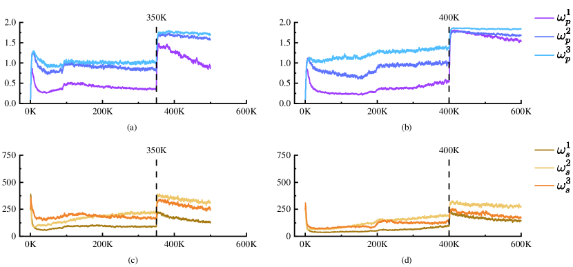
Figure 4: Adaptation processes of TPL and TSL. (a) and (c) are weight adaptations of TPL and TSL on the CelebA dataset, where $\omega_{p}^{1}$, $\omega_{p}^{2}$ and $\omega_{p}^{3}$ are weights of TPL corresponding to the first, second and third max-pooling layers of the VGG-16 network respectively. (b) and (d) show how weights of TPL and TSL adapt on Paris StreetView dataset. $\omega_{s}^{1}$, $\omega_{s}^{2}$ and $\omega_{s}^{3}$ denote the weights of TSL, and they also correspond to the first three max-pooling layers of the VGG-16 network, in shallow to deep manner.

TABLE IV: Quantitative Results Of two base models trained by customary settings and our framework on CelebA dataset. The Best Results Are Boldfaced. ^↑ Means Higher Is Better. Ours means the model is trained by our framework. ^↓ Means Lower Is Better.

Metric	Mask	PRVS	Ours	EG2	Ours
PSNR ↑	(0.1,0.2]	31.860	32.191	33.747	34.072
	(0.2,0.3]	28.633	28.989	31.164	31.477
	(0.3,0.4]	26.373	26.737	29.352	29.669
	(0.4,0.5]	24.525	24.886	27.860	28.186
	(0.5,0.6]	21.750	22.045	25.611	25.879
SSIM ↑	(0.1,0.2]	0.9684	0.9694	0.9758	0.9775
	(0.2,0.3]	0.9417	0.9435	0.9587	0.9616
	(0.3,0.4]	0.9113	0.9141	0.9405	0.9449
	(0.4,0.5]	0.8767	0.8807	0.9207	0.9271
	(0.5,0.6]	0.8148	0.8210	0.8890	0.8985
MAE ↓	(0.1,0.2]	0.0066	0.0065	0.0059	0.0057
	(0.2,0.3]	0.0120	0.0118	0.0100	0.0096
	(0.3,0.4]	0.0179	0.0178	0.0142	0.0137
	(0.4,0.5]	0.0249	0.0249	0.0189	0.0183
	(0.5,0.6]	0.0394	0.0388	0.0273	0.0266
LPIPS ↓	(0.1,0.2]	0.0362	0.0305	0.0231	0.0231
	(0.2,0.3]	0.0678	0.0558	0.0401	0.0397
	(0.3,0.4]	0.1034	0.0842	0.0585	0.0575
	(0.4,0.5]	0.1435	0.1164	0.0787	0.0771
	(0.5,0.6]	0.2138	0.1720	0.1092	0.1070
FID ↓	(0.1,0.2]	1.7208	1.4015	1.0978	1.0225
	(0.2,0.3]	4.4684	3.4639	2.3558	2.2207
	(0.3,0.4]	8.7892	6.7080	4.0951	3.8143
	(0.4,0.5]	15.341	11.692	6.5822	6.1479
	(0.5,0.6]	27.478	23.910	10.725	10.017

TABLE V: Quantitative Results Of two base models trained by customary settings and our framework on Paris StreetView dataset. Ours means the model is trained with our framework. The Best Results Are Boldfaced. ^↑ Means Higher Is Better. ^↓ Means Lower Is Better.

Metric	Mask	PRVS	Ours	EG2	Ours
PSNR ↑	(0.1,0.2]	31.380	31.391	33.282	33.417
	(0.2,0.3]	28.354	28.451	30.895	30.992
	(0.3,0.4]	26.241	26.488	29.151	29.271
	(0.4,0.5]	24.126	24.690	27.547	27.692
	(0.5,0.6]	21.419	22.214	25.159	25.201
SSIM ↑	(0.1,0.2]	0.9565	0.9565	0.9694	0.9701
	(0.2,0.3]	0.9233	0.9242	0.9489	0.9504
	(0.3,0.4]	0.8835	0.8867	0.9260	0.9285
	(0.4,0.5]	0.8315	0.8395	0.8990	0.9028
	(0.5,0.6]	0.7446	0.7647	0.8517	0.8556
MAE ↓	(0.1,0.2]	0.0120	0.0120	0.0106	0.0105
	(0.2,0.3]	0.0173	0.0171	0.0144	0.0143
	(0.3,0.4]	0.0235	0.0229	0.0184	0.0182
	(0.4,0.5]	0.0320	0.0304	0.0236	0.0232
	(0.5,0.6]	0.0477	0.0432	0.0328	0.0326
LPIPS ↓	(0.1,0.2]	0.0881	0.0490	0.0367	0.0364
	(0.2,0.3]	0.1133	0.0804	0.0545	0.0539
	(0.3,0.4]	0.1455	0.1173	0.0749	0.0732
	(0.4,0.5]	0.1931	0.1666	0.1006	0.0988
	(0.5,0.6]	0.2750	0.2445	0.1396	0.1373
FID ↓	(0.1,0.2]	22.778	23.682	18.941	18.528
	(0.2,0.3]	35.892	36.941	27.415	27.301
	(0.3,0.4]	48.371	47.383	36.976	35.401
	(0.4,0.5]	68.103	65.068	45.613	45.466
	(0.5,0.6]	99.863	87.485	58.323	58.767

Universality of AWA. We also apply our framework to train various SOTA methods [25, 26] on Paris StreetView and CelebA datasets. As EG has two generators and only the image generator (EG2) is trained by perceptual and style losses, we choose EG2 for experiments. As presented in TABLE IV and TABLE V, AWA can consistently improve the inpainting performance of SOTA methods. This indicates that AWA is not limited to one specific inpainting architecture but can be easily generalized to help improve the ability of auxiliary losses for image inpainting.

Weight Adaptation Processes. It is also insightful to observe how auxiliary weights adapt during training processes. Models here are CTSDG trained by our framework. Fig. 4 show the adaption processes of TPL and TSL on CelebA and Paris StreetView datasets. It is obvious that all weights increase at the start of fine-tune stage (350,000 for CelebA and 400,000 for Paris StreetView), which reveals that deep feature based auxiliary losses are more useful in the fine-tune stage. As Fig. 4(a) and Fig. 4 (b) show, $\omega_{p}^{1}$ is the smallest while $\omega_{p}^{3}$ is the largest. This indicates that loss terms of shallower features are paid less attention. The similar phenomena can also be found in the adaptation processes of TSL (Fig. 4(c) and Fig. 4(d)). We conjecture that deeper features are more useful for TPL and TSL to train inpainting generators.

VI Discussions and Future Work

In this paper, we propose an auxiliary loss reweighting framework for image inpainting, which train inpainting generators with better auxiliary losses and efficiently reweight auxiliary losses without time-consuming grid search. Specifically, we propose TPL and TSL to increase the effectiveness of standard perceptual loss and style loss by independently weighting different loss terms of different deep features. We further design the AWA algorithm to dynamically adjusts the parameters of TPL and TSL in a single training process. Our framework is effective and generalizes well for the existing image inpainting models.

Though the proposed framework is efficient in image inpainting, the magnitude of auxiliary parameters is restricted by the requirement of computing Jacobian matrices in the auxiliary update process. In effect, the computational cost linearly increases as the number of auxiliary parameters grows.

We believe that our approach is one step toward a simple and general auxiliary loss adaptation framework that could dynamically reweight auxiliary losses for inpainting models with better performance and less computational cost. Extending such capacity to other tasks and increasing the flexibility of our method is ongoing.

Here we prove that the surrogate loss function equals $\mathcal{L}_{c}$ by verifying that they share the same gradient directions with respect to auxiliary parameters of TPL and TSL. Recall that the original objective for auxiliary parameters is shown in Eq. 7. We first compute the gradient of $\mathcal{L}_{c}$ in Eq. 7 with respect to auxiliary paramters. More formally, compute $\nabla_{\phi_{p}}\mathcal{L}_{c}(\theta^{K})$ and $\nabla_{\phi_{s}}\mathcal{L}_{c}(\theta^{K})$. Based on chain rules:

$$\nabla_{\phi_{p}}\mathcal{L}_{c}(\theta^{K})=\mathop{\underbrace{\nabla_{\theta^{K}}\mathcal{L}_{c}(\theta^{K})}}_{1\times|\theta|}\mathop{\underbrace{J_{\theta^{K}}(\omega_{p})}}_{|\theta|\times|\omega_{p}|}\mathop{\underbrace{J_{\omega_{p}}(\phi_{p})}}_{|\omega_{p}|\times|\phi_{p}|},$$ (A1)

$$\nabla_{\phi_{s}}\mathcal{L}_{c}(\theta^{K})=\mathop{\underbrace{\nabla_{\theta^{K}}\mathcal{L}_{c}(\theta^{K})}}_{1\times|\theta|}\mathop{\underbrace{J_{\theta^{K}}(\omega_{s})}}_{|\theta|\times|\omega_{s}|}\mathop{\underbrace{J_{\omega_{s}}(\phi_{s})}}_{|\omega_{s}|\times|\phi_{s}|}.$$ (A2)

Next, we compute Jacobian matrices of $\theta^{K}$ with respect to auxiliary weights $\omega_{p}$ and $\omega_{s}$. Following the definition of the Jacobian matrix, the element at location $(a,b)$ of $J_{\theta^{K}}(\omega_{p})$ denoted as $J_{\theta^{K}}(\omega_{p})_{(a,b)}$, which can be computed as follows:

$$J_{\theta^{K}}(\omega_{p})_{(a,b)}=\frac{\partial(\theta^{K})_{a}}{\partial(\omega_{p})_{b}}$$ (A3)

$$=\frac{\partial\left(\theta-\alpha\sum_{j=1}^{K}{\left(\lambda_{m}^{T}J_{m}\left(\theta^{j}\right)+\omega_{p}^{T}J_{p}\left(\theta^{j}\right)+\omega_{s}^{T}J_{s}\left(\theta^{j}\right)\right)}\right)_{a}}{\partial\left(\omega_{p}\right)_{b}}$$

$$=-\alpha\sum_{j=1}^{K}\frac{\partial\left({\omega_{p}^{T}J_{p}\left(\theta^{j}\right)}\right)_{a}}{\partial\left(\omega_{p}\right)_{b}}$$

$$=-\alpha\sum_{j=1}^{K}J_{p}(\theta^{j})_{(b,a)}.$$

The elements of $J_{\theta^{K}}(\omega_{p})$ shares the same computational process:

$$J_{\theta^{K}}(\omega_{s})_{(a,b)}=\frac{\partial(\theta^{K})_{a}}{\partial(\omega_{s})_{b}}$$ (A4)

$$=\frac{\partial\left(\theta-\alpha\sum_{j=1}^{K}{\left(\lambda_{m}^{T}J_{m}\left(\theta^{j}\right)+\omega_{p}^{T}J_{p}\left(\theta^{j}\right)+\omega_{s}^{T}J_{s}\left(\theta^{j}\right)\right)}\right)_{a}}{\partial\left(\omega_{s}\right)_{b}}$$

$$=-\alpha\sum_{j=1}^{K}\frac{\partial\left({\omega_{s}^{T}J_{s}\left(\theta^{j}\right)}\right)_{a}}{\partial\left(\omega_{s}\right)_{b}}$$

$$=-\alpha\sum_{j=1}^{K}J_{s}(\theta^{j})_{(b,a)}.$$

Such that these Jacobian matrices are:

$$J_{\theta^{K}}(\omega_{p})=-\alpha\sum_{j=1}^{K}J_{p}^{T}(\theta^{j}),$$ (A5)

$$J_{\theta^{K}}(\omega_{s})=-\alpha\sum_{j=1}^{K}J_{s}^{T}(\theta^{j}).$$ (A6)

Then, combining Eq. A1, Eq. A5, we get the explicit gradient of $\mathcal{L}_{c}$ with respect to auxiliary parameters of TPL.

$$\nabla_{\phi_{p}}\mathcal{L}_{c}(\theta^{K})= \nabla_{\theta^{K}}\mathcal{L}_{c}(\theta^{K})J_{\theta^{K}}(\omega_{p})J_{\omega_{p}}(\phi_{p})$$ (A7)

$$=-\alpha\nabla_{\theta^{K}}\mathcal{L}_{c}(\theta^{K})\sum_{j=1}^{K}J_{p}^{T}(\theta^{j})J_{\omega_{p}}(\phi_{p}),$$

$$\nabla_{\phi_{s}}\mathcal{L}_{c}(\theta^{K})= \nabla_{\theta^{K}}\mathcal{L}_{c}(\theta^{K})J_{\theta^{K}}(\omega_{s})J_{\omega_{s}}(\phi_{s})$$ (A8)

$$=-\alpha\nabla_{\theta^{K}}\mathcal{L}_{c}(\theta^{K})\sum_{j=1}^{K}J_{s}^{T}(\theta^{j})J_{\omega_{s}}(\phi_{s}).$$

Finally, let’s verify that the gradients of the surrogate loss in Eq. 8 share the same directions of the gradients of $\mathcal{L}_{c}$.

$$\nabla_{\phi_{p}}\mathcal{L}_{c}(\theta^{K}) \propto{\nabla_{\phi_{p}}}\mathcal{L}_{sg}(\phi_{p},\phi_{s})$$ (A9)

$$=-\nabla_{\theta}\mathcal{L}_{c}(\theta^{K})\sum_{j}J_{p}(\theta^{j})J_{\omega_{p}}(\phi_{p}),$$

$$\nabla_{\phi_{s}}\mathcal{L}_{c}(\theta^{K}) \propto{\nabla_{\phi_{p}}}\mathcal{L}_{sg}(\phi_{s},\phi_{s})$$ (A10)

$$=-\nabla_{\theta}\mathcal{L}_{c}(\theta^{K})\sum_{j}J_{s}(\theta^{j})J_{\omega_{s}}(\phi_{s}),$$

References

- [1] J. Li, N. Wang, L. Zhang, B. Du, and D. Tao, “Recurrent feature reasoning for image inpainting,” in Proceedings of the IEEE/CVF Conference on Computer Vision and Pattern Recognition, 2020, pp. 7760–7768.
- [2] Z. Liu, P. Luo, X. Wang, and X. Tang, “Large-scale celebfaces attributes (celeba) dataset,” Retrieved August, vol. 15, p. 2018, 2018.
- [3] Y. Jo and J. Park, “Sc-fegan: Face editing generative adversarial network with user’s sketch and color,” in Proceedings of the IEEE/CVF international conference on computer vision, 2019, pp. 1745–1753.
- [4] R. Uittenbogaard, C. Sebastian, J. Vijverberg, B. Boom, D. M. Gavrila et al., “Privacy protection in street-view panoramas using depth and multi-view imagery,” in Proceedings of the IEEE/CVF Conference on Computer Vision and Pattern Recognition, 2019, pp. 10 581–10 590.
- [5] C. Barnes, E. Shechtman, A. Finkelstein, and D. B. Goldman, “Patchmatch: A randomized correspondence algorithm for structural image editing,” ACM Trans. Graph., vol. 28, no. 3, p. 24, 2009.
- [6] I. Drori, D. Cohen-Or, and H. Yeshurun, “Fragment-based image completion,” in ACM SIGGRAPH 2003 Papers, 2003, pp. 303–312.
- [7] C. Ballester, M. Bertalmio, V. Caselles, G. Sapiro, and J. Verdera, “Filling-in by joint interpolation of vector fields and gray levels,” 2001.
- [8] D. Pathak, P. Krahenbuhl, J. Donahue, T. Darrell, and A. A. Efros, “Context encoders: Feature learning by inpainting,” in Proceedings of the IEEE conference on computer vision and pattern recognition, 2016, pp. 2536–2544.
- [9] J. Yu, Z. Lin, J. Yang, X. Shen, X. Lu, and T. S. Huang, “Free-form image inpainting with gated convolution,” in Proceedings of the IEEE International Conference on Computer Vision, 2019, pp. 4471–4480.
- [10] ——, “Generative image inpainting with contextual attention,” in Proceedings of the IEEE Conference on Computer Vision and Pattern Recognition, 2018, pp. 5505–5514.
- [11] X. Guo, H. Yang, and D. Huang, “Image inpainting via conditional texture and structure dual generation,” in Proceedings of the IEEE/CVF International Conference on Computer Vision, 2021, pp. 14 134–14 143.
- [12] M. Heusel, H. Ramsauer, T. Unterthiner, B. Nessler, and S. Hochreiter, “Gans trained by a two time-scale update rule converge to a local nash equilibrium,” in Neural Information Processing Systems (NIPS), 2017.
- [13] N. Wang, Y. Zhang, and L. Zhang, “Dynamic selection network for image inpainting,” IEEE Transactions on Image Processing, vol. 30, pp. 1784–1798, 2021.
- [14] M. Zhu, D. He, X. Li, C. Li, F. Li, X. Liu, E. Ding, and Z. Zhang, “Image inpainting by end-to-end cascaded refinement with mask awareness,” IEEE Transactions on Image Processing, vol. 30, pp. 4855–4866, 2021.
- [15] L. A. Gatys, A. S. Ecker, and M. Bethge, “A neural algorithm of artistic style,” arXiv preprint arXiv:1508.06576, 2015.
- [16] O. Russakovsky, J. Deng, H. Su, J. Krause, S. Satheesh, S. Ma, Z. Huang, A. Karpathy, A. Khosla, M. Bernstein et al., “Imagenet large scale visual recognition challenge,” International journal of computer vision, vol. 115, no. 3, pp. 211–252, 2015.
- [17] K. Simonyan and A. Zisserman, “Very deep convolutional networks for large-scale image recognition,” arXiv preprint arXiv:1409.1556, 2014.
- [18] V. Kwatra, I. Essa, A. Bobick, and N. Kwatra, “Texture optimization for example-based synthesis,” in ACM SIGGRAPH 2005 Papers, 2005, pp. 795–802.
- [19] T. Barbu, “Variational image inpainting technique based on nonlinear second-order diffusions,” Computers & Electrical Engineering, vol. 54, pp. 345–353, 2016.
- [20] A. Bertozzi and C.-B. Schönlieb, “Unconditionally stable schemes for higher order inpainting,” Communications in Mathematical Sciences, vol. 9, no. 2, pp. 413–457, 2011.
- [21] T. F. Chan and J. Shen, “Nontexture inpainting by curvature-driven diffusions,” Journal of visual communication and image representation, vol. 12, no. 4, pp. 436–449, 2001.
- [22] J. Shen, S. H. Kang, and T. F. Chan, “Euler’s elastica and curvature-based inpainting,” SIAM journal on Applied Mathematics, vol. 63, no. 2, pp. 564–592, 2003.
- [23] G. Sridevi and S. Srinivas Kumar, “Image inpainting based on fractional-order nonlinear diffusion for image reconstruction,” Circuits, Systems, and Signal Processing, vol. 38, no. 8, pp. 3802–3817, 2019.
- [24] G. Liu, F. A. Reda, K. J. Shih, T.-C. Wang, A. Tao, and B. Catanzaro, “Image inpainting for irregular holes using partial convolutions,” in Proceedings of the European Conference on Computer Vision (ECCV), 2018, pp. 85–100.
- [25] K. Nazeri, E. Ng, T. Joseph, F. Z. Qureshi, and M. Ebrahimi, “Edgeconnect: Generative image inpainting with adversarial edge learning,” arXiv preprint arXiv:1901.00212, 2019.
- [26] J. Li, F. He, L. Zhang, B. Du, and D. Tao, “Progressive reconstruction of visual structure for image inpainting,” in Proceedings of the IEEE/CVF International Conference on Computer Vision, 2019, pp. 5962–5971.
- [27] R. A. Yeh, C. Chen, T. Yian Lim, A. G. Schwing, M. Hasegawa-Johnson, and M. N. Do, “Semantic image inpainting with deep generative models,” in Proceedings of the IEEE conference on computer vision and pattern recognition, 2017, pp. 5485–5493.
- [28] A. Lahiri, A. K. Jain, S. Agrawal, P. Mitra, and P. K. Biswas, “Prior guided gan based semantic inpainting,” in Proceedings of the IEEE/CVF Conference on Computer Vision and Pattern Recognition, 2020, pp. 13 696–13 705.
- [29] H. Liu, Z. Wan, W. Huang, Y. Song, X. Han, and J. Liao, “Pd-gan: Probabilistic diverse gan for image inpainting,” in Proceedings of the IEEE/CVF Conference on Computer Vision and Pattern Recognition, 2021, pp. 9371–9381.
- [30] Z. Yi, Q. Tang, S. Azizi, D. Jang, and Z. Xu, “Contextual residual aggregation for ultra high-resolution image inpainting,” in Proceedings of the IEEE/CVF Conference on Computer Vision and Pattern Recognition, 2020, pp. 7508–7517.
- [31] Y. Song, C. Yang, Y. Shen, P. Wang, Q. Huang, and C.-C. J. Kuo, “Spg-net: Segmentation prediction and guidance network for image inpainting,” arXiv preprint arXiv:1805.03356, 2018.
- [32] H. Liu, B. Jiang, Y. Xiao, and C. Yang, “Coherent semantic attention for image inpainting,” in Proceedings of the IEEE/CVF International Conference on Computer Vision, 2019, pp. 4170–4179.
- [33] M. Suin, K. Purohit, and A. Rajagopalan, “Distillation-guided image inpainting,” in Proceedings of the IEEE/CVF International Conference on Computer Vision, 2021, pp. 2481–2490.
- [34] W. Xiong, J. Yu, Z. Lin, J. Yang, X. Lu, C. Barnes, and J. Luo, “Foreground-aware image inpainting,” in Proceedings of the IEEE conference on computer vision and pattern recognition, 2019, pp. 5840–5848.
- [35] Y. Yu, F. Zhan, S. Lu, J. Pan, F. Ma, X. Xie, and C. Miao, “Wavefill: A wavelet-based generation network for image inpainting,” in Proceedings of the IEEE/CVF International Conference on Computer Vision, 2021, pp. 14 114–14 123.
- [36] C. Cao and Y. Fu, “Learning a sketch tensor space for image inpainting of man-made scenes,” in Proceedings of the IEEE/CVF International Conference on Computer Vision, 2021, pp. 14 509–14 518.
- [37] D. Ding, S. Ram, and J. J. Rodríguez, “Image inpainting using nonlocal texture matching and nonlinear filtering,” IEEE Transactions on Image Processing, vol. 28, no. 4, pp. 1705–1719, 2018.
- [38] D. Ding, S. Ram, and J. J. Rodriguez, “Perceptually aware image inpainting,” Pattern Recognition, vol. 83, pp. 174–184, 2018.
- [39] H. Su, V. Jampani, D. Sun, O. Gallo, E. Learned-Miller, and J. Kautz, “Pixel-adaptive convolutional neural networks,” in Proceedings of the IEEE/CVF Conference on Computer Vision and Pattern Recognition, 2019, pp. 11 166–11 175.
- [40] J. Yang, Z. Qi, and Y. Shi, “Learning to incorporate structure knowledge for image inpainting,” in Proceedings of the AAAI Conference on Artificial Intelligence, vol. 34, no. 07, 2020, pp. 12 605–12 612.
- [41] S. Iizuka, E. Simo-Serra, and H. Ishikawa, “Globally and locally consistent image completion,” ACM Transactions on Graphics (ToG), vol. 36, no. 4, pp. 1–14, 2017.
- [42] T. Yu, Z. Guo, X. Jin, S. Wu, Z. Chen, W. Li, Z. Zhang, and S. Liu, “Region normalization for image inpainting.” in AAAI, 2020, pp. 12 733–12 740.
- [43] R. Caruana, “Multitask learning,” Machine learning, vol. 28, no. 1, pp. 41–75, 1997.
- [44] S. Thrun and L. Pratt, Learning to learn. Springer Science & Business Media, 2012.
- [45] S. Ruder, “An overview of multi-task learning in deep neural networks,” arXiv preprint arXiv:1706.05098, 2017.
- [46] R. K. Ando, T. Zhang, and P. Bartlett, “A framework for learning predictive structures from multiple tasks and unlabeled data.” Journal of Machine Learning Research, vol. 6, no. 11, 2005.
- [47] O. Sener and V. Koltun, “Multi-task learning as multi-objective optimization,” Advances in neural information processing systems, vol. 31, 2018.
- [48] R. Girshick, “Fast r-cnn,” in Proceedings of the IEEE international conference on computer vision, 2015, pp. 1440–1448.
- [49] S. Sharma and B. Ravindran, “Online multi-task learning using active sampling,” 2017.
- [50] Z. Chen, V. Badrinarayanan, C.-Y. Lee, and A. Rabinovich, “Gradnorm: Gradient normalization for adaptive loss balancing in deep multitask networks,” in International Conference on Machine Learning. PMLR, 2018, pp. 794–803.
- [51] A. Kendall, Y. Gal, and R. Cipolla, “Multi-task learning using uncertainty to weigh losses for scene geometry and semantics,” in Proceedings of the IEEE conference on computer vision and pattern recognition, 2018, pp. 7482–7491.
- [52] G. Huang, D. Chen, T. Li, F. Wu, L. Van Der Maaten, and K. Q. Weinberger, “Multi-scale dense convolutional networks for efficient prediction,” arXiv preprint arXiv:1703.09844, vol. 2, 2017.
- [53] H. Hu, D. Dey, M. Hebert, and J. A. Bagnell, “Learning anytime predictions in neural networks via adaptive loss balancing,” in Proceedings of the AAAI Conference on Artificial Intelligence, vol. 33, no. 01, 2019, pp. 3812–3821.
- [54] Y. Du, W. M. Czarnecki, S. M. Jayakumar, M. Farajtabar, R. Pascanu, and B. Lakshminarayanan, “Adapting auxiliary losses using gradient similarity,” arXiv preprint arXiv:1812.02224, 2018.
- [55] X. Lin, H. S. Baweja, G. Kantor, and D. Held, “Adaptive auxiliary task weighting for reinforcement learning,” Advances in neural information processing systems, vol. 32, 2019.
- [56] B. Shi, J. Hoffman, K. Saenko, T. Darrell, and H. Xu, “Auxiliary task reweighting for minimum-data learning,” Advances in Neural Information Processing Systems, vol. 33, pp. 7148–7160, 2020.
- [57] D. P. Kingma and J. Ba, “Adam: A method for stochastic optimization,” arXiv preprint arXiv:1412.6980, 2014.
- [58] C. Doersch, S. Singh, A. Gupta, J. Sivic, and A. Efros, “What makes paris look like paris?” ACM Transactions on Graphics, vol. 31, no. 4, 2012.
- [59] B. Zhou, A. Lapedriza, A. Khosla, A. Oliva, and A. Torralba, “Places: A 10 million image database for scene recognition,” IEEE transactions on pattern analysis and machine intelligence, vol. 40, no. 6, pp. 1452–1464, 2017.
- [60] C. Zheng, T.-J. Cham, and J. Cai, “Pluralistic image completion,” in Proceedings of the IEEE Conference on Computer Vision and Pattern Recognition, 2019, pp. 1438–1447.
- [61] R. Zhang, P. Isola, A. A. Efros, E. Shechtman, and O. Wang, “The unreasonable effectiveness of deep features as a perceptual metric,” in Proceedings of the IEEE conference on computer vision and pattern recognition, 2018, pp. 586–595.
- [62] M. Heusel, H. Ramsauer, T. Unterthiner, B. Nessler, and S. Hochreiter, “Gans trained by a two time-scale update rule converge to a local nash equilibrium,” arXiv preprint arXiv:1706.08500, 2017.
- [63] H. Hu, D. Dey, M. Hebert, and J. A. Bagnell, “Learning anytime predictions in neural networks via adaptive loss balancing,” in Proceedings of the AAAI Conference on Artificial Intelligence, vol. 33, no. 01, 2019, pp. 3812–3821.