Linear, or Non-Linear, That is the Question!

Abstract.

There were fierce debates on whether the non-linear embedding propagation of GCNs is appropriate to GCN-based recommender systems. It was recently found that the linear embedding propagation shows better accuracy than the non-linear embedding propagation. Since this phenomenon was discovered especially in recommender systems, it is required that we carefully analyze the linearity and non-linearity issue. In this work, therefore, we revisit the issues of i) which of the linear or non-linear propagation is better and ii) which factors of users/items decide the linearity/non-linearity of the embedding propagation. We propose a novel Hybrid Method of Linear and non-linEar collaborative filTering method (, pronounced as Hamlet). In our design, there exist both linear and non-linear propagation steps, when processing each user or item node, and our gating module chooses one of them, which results in a hybrid model of the linear and non-linear GCN-based collaborative filtering (CF). The proposed model yields the best accuracy in three public benchmark datasets. Moreover, we classify users/items into the following three classes depending on our gating modules’ selections: Full-Non-Linearity (FNL), Partial-Non-Linearity (PNL), and Full-Linearity (FL). We found that there exist strong correlations between nodes’ centrality and their class membership,  important user/item nodes exhibit more preferences towards the non-linearity during the propagation steps. To our knowledge, we are the first who design a hybrid method and report the correlation between the graph centrality and the linearity/non-linearity of nodes. All codes and datasets are available at: https://github.com/qbxlvnf11/HMLET.

1. Introduction

Recommender systems, personalized information filtering (IF) technologies, can be applied to many services, ranging from E-commerce, advertising, and social media to many other online and offline service platforms (Ying et al., 2018). One of the most popular recommender systems, collaborative filtering (CF), provides personalized preferred items to users by learning user and item embeddings from their historical user-item interactions (Ebesu et al., 2018; He et al., 2017; Hu et al., 2008; Koren et al., 2009; Rendle et al., 2009; Wang et al., 2014; Chae et al., 2018; Lee et al., 2018; Chae et al., 2020; Choi et al., 2021).

One of the mainstream research directions in recommender systems is how to learn high-order connectivity of user-item interactions while filtering out noises. Recently, GCN-based CF methods became popular in recommender systems because they show strong points to capture such latent high-order connectivity. Since existing GCNs are originally designed for graph or node classification tasks on attributed graphs, however, two limitations had been raised out when it comes to GCN-based CF methods: training difficulty (Wu et al., 2019b; Chen et al., 2020b; He et al., 2020a) and over-smoothing (Chen et al., 2020a, b; He et al., 2020a). Over-smoothing degrades the recommendation accuracy by considering the connectivity information too much (Chen et al., 2020b). To overcome these problems, a couple of linear GCNs (linear embedding propagation-based GCNs) were proposed (Chen et al., 2020b; He et al., 2020a). These methods effectively alleviate the aforementioned two limitations and show superior performance over non-linear GCNs (non-linear embedding propagation-based GCNs). Even though linear GCNs show the state-of-the-art performance in many benchmark CF datasets, it is questionable in our opinion whether they can properly handle users and items with various characteristics and whether linear GCNs are consistently superior to non-linear GCNs in all cases. In addition, we are curious about, if one outperforms the other, which factors of graphs decide it.

To this end, we propose a Hybrid Method of Linear and non-linEar collaborative filTering (, pronounced as Hamlet), a GCN-based CF method. has the following key design points: i) We adopt a gating concept to decide between the linear and non-linear propagation for each node in a layer. ii) We perform residual prediction, where the embeddings from all layers are aggregated and used collectively for final predictions. Therefore, we let our gating modules decide which of the linear or non-linear propagation is used for a certain node at a certain layer instead of relying on manually designed architectures. This gating mechanism’s key point is how to generate appropriate one-hot vectors. For this purpose, we adopt the Gumbel-softmax (Gumbel, 1954; Maddison et al., 2014).

To our knowledge, we are the first who combines the linear and non-linear embedding propagation in a systematic way,  via the gating in our paper. Our gating mechanism can be considered as a sort of neural architecture search (NAS) for the GCN-based CF method. However, our proposed mechanism is more sophisticated because it provides the switching function for each user/item and the overall GCN architecture can be varied from a node’s perspective to another.

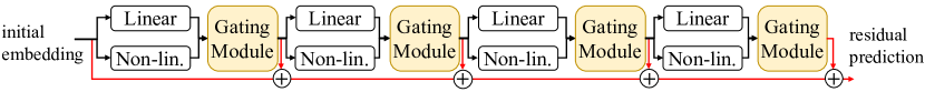
(a) HMLET(All)

(b) HMLET(Front)

(c) HMLET(Middle)

(d) HMLET(End)

Figure 1. Four variants of in terms of the location of the non-linear propagation. HMLET(End) shows the best accuracy in our experiments. It was known that the problem of over-smoothing happens with more than 2 non-linear propagation layers, and we use up to 2 non-linear layers.

We conduct experiments with three benchmark CF datasets and compare our with various state-of-the-art CF methods in terms of the normalized discounted cumulative gain (NDCG), recall, and precision. We also define several variations of in terms of the locations of the non-linear propagation layers (see Fig. 1). Among all of them, HMLET(End) shows the best performance in all datasets. Furthermore, we define three classes of nodes,  users and items, depending on their preferences on the linear or non-linear propagation: Full-Non-Linearity (FNL), Partial-Non-Linearity (PNL), and Full-Linearity (FL). An FNL (resp. FL) node means that our gating module chooses the non-linear (resp. linear) propagation every time for the node and a PNL node has a mixed characteristic. At the end, we analyze the class-specific characteristics in terms of various graph centrality metrics and reveal that there exist strong correlations between the graph centrality,   the role of a node in a graph, and the linear/non-linear gating outcomes (see Table 1). Our discovery shows that recommendation datasets are complicated because the linearity and non-linearity are mixed.

Contributions of our paper can be summarized as follows:

• We propose , which dynamically selects the best propagation method for each node in a layer.

• We reveal that the role of a node in a graph is closely related to its linearity/non-linearity, e.g.,  our gating module prefers the non-linear embedding propagation for the nodes with strong connections to other nodes.

• Our experiments on three benchmark datasets show that outperforms baselines in yielding better performance.

Table 1. The characteristics of node classes in terms of various metrics. FNL (resp. FL) means a class of nodes for which our gating modules select only the non-linear (resp. linear) propagation in all layers. For PNL, our gating modules choose different propagation methods in different layers.

Class	Degree	PageRank	Betweenness	Closeness
FNL	High	High	High	High
PNL	Moderate	Moderate	Moderate	Moderate
FL	Low	Low	Low	Low

2. Related Works

In this section, we review recommender systems and the Gumbel-softmax used in our proposed gating module.

2.1. Recommender Systems

Traditional recommender systems have focused on matrix factorization (MF) techniques (Koren et al., 2009; Hwang et al., 2016). Typical MF-based methods include BPR (Rendle et al., 2009) and WRMF (Hu et al., 2008). These MF-based methods simply learn relationships between users and items via dot products. Therefore, they have limitations in considering potentially complex relationships between users and items inherent in user-item interactions (He et al., 2017). To overcome these limitations, deep learning-based recommender systems, e.g., Autoencoders (Kingma and Welling, 2013; Vincent et al., 2008) and GCNs (Bruna et al., 2014; Kipf and Welling, 2017; Wu et al., 2019b; Hamilton et al., 2017), have been proposed to effectively learn more complicated relationships between users and items (Wang et al., 2019; Ying et al., 2018; Zhang et al., 2020; van den Berg et al., 2018).

Recently, recommender systems using GCNs (Wang et al., 2019; Ying et al., 2018; van den Berg et al., 2018) are gathering much attention. GCN-based methods can effectively learn the behavioral patterns between users and items by directly capturing the collaborative signals inherent in the user-item interactions (Wang et al., 2019). Typical GCN-based methods include GC-MC (van den Berg et al., 2018), PinSage (Ying et al., 2018), and NGCF (Wang et al., 2019). In general, GCN-based methods model a set of user-item interactions as a user-item bipartite graph and then perform the following three steps:

(Step 1) Initialization Step: They randomly set the initial $D$-dimensional embedding $\bm{e}^{0}$ of all user $u$ and item $v$,  $\bm{e}_{u}^{0},\bm{e}_{v}^{0}\in\mathbb{R}^{D}$.

(Step 2) Propagation Step: First of all, this propagation step is iterated $K$ times,   $K$ layers of embedding propagation. Given the $K$ layers, the embedding of a user node $u$ (resp. an item node $v$) in $i$-th layer is updated based on the embeddings of $u$’s (resp. $v$’s) neighbors $N_{u}$ (resp. $N_{v}$) in ($i-1$)-th layer as follows:

(1) $$\begin{split}\bm{e}_{u}^{i}=\sigma(\Sigma_{v\in N_{u}}\bm{e}_{v}^{i-1}\bm{W}_{i}),\;\;\;\bm{e}_{v}^{i}=\sigma(\Sigma_{u\in N_{v}}\bm{e}_{u}^{i-1}\bm{W}_{i}),\end{split}$$

where $\sigma$ denotes a non-linear activation function, e.g., ReLU, and $\bm{W}_{i}\in\mathbb{R}^{D\times D}$ is a trainable transformation matrix. There exist some other variations: i) including the self-embeddings,  $N_{u}=N_{u}\cup\{u\}$ and $N_{v}=N_{v}\cup\{v\}$, ii) removing the transformation matrix, and iii) removing the non-linear activation function, which is in particular called as linear propagation (Chen et al., 2020b; He et al., 2020a).

(Step 3) Prediction Step: The preference of user $u$ to item $v$ is typically predicted using the dot product between the user $u$’s and item $v$’s embeddings in the last layer $K$,  $\hat{r}_{u,v}=\bm{e}_{u}^{K}\odot\bm{e}_{v}^{K}$.

However, these GCN-based methods have two limitations: i) training difficulty  (Wu et al., 2019b; Chen et al., 2020b; He et al., 2020a) and ii) over-smoothing,  too similar embeddings of nodes (Chen et al., 2020a, b; He et al., 2020a). First, the training difficulty is caused by their use of a non-linear activation function in the propagation step (Wu et al., 2019b; Chen et al., 2020b; He et al., 2020a). Specifically, the non-linear activation function complicates the propagation step, and even worse, this operation is repeatedly performed whenever a new layer is created. Thus, they suffer from the training difficulty of the non-linear activation functions for large-scale user-item bipartite graphs  (Wu et al., 2019b; Chen et al., 2020b).

Next, the over-smoothing is caused as they use only the embeddings updated through the last layer in the prediction layer (Chen et al., 2020b). Specifically, as the number of layers increases, the embedding of a node will be influenced more from its neighbors’ embeddings. As a result, the embedding of a node in the last layer becomes similar to the embeddings of many directly/indirectly connected nodes (Chen et al., 2020b, a). This phenomenon prevents most of the existing GCN-based methods from effectively utilizing the information of high-order neighborhood. Empirically, this is also shown by the fact that most of non-linear GCN-based methods show better performance when using only a few layers instead of deep networks.

Recently, LR-GCCF (Chen et al., 2020b) and LightGCN (He et al., 2020a), which are GCN-based recommender systems to alleviate the problems, have been proposed. First, to alleviate the former problem, they perform a linear embedding propagation without using a non-linear activation function in the propagation step. In order to mitigate the latter problem, they utilize the embeddings from all layers for prediction. After that, they perform residual prediction (Chen et al., 2020b; He et al., 2020a), which predict each user’s preference to each item with the multiple embeddings from the multiple layers. In (Chen et al., 2020b; He et al., 2020a), the authors demonstrated that a GCN architecture with the linear embedding propagation and the residual prediction can significantly improve the recommendation accuracy by successfully addressing the two problems.

Table 2. GCN-based recommender systems. In each layer, the gating module in chooses either of the linear or the non-linear propagation for each node.

	GC-MC	PinSage	NGCF	LR-GCCF	LightGCN
Non-Linear Propagation	O	O	O	X	X	O
Linear Propagation	X	X	X	O	O	O
Residual Prediction	X	X	O	O	O	O

In summary, GCN-based recommender systems can be characterized by, as shown in Table 2, the propagation and prediction types. We note that all existing methods consider only one of the linear or non-linear propagation,   they assume only one type of user-item interactions. However, we conjecture that user-item interactions are neither only linear nor only non-linear, for which we will conduct in-depth analyses in Section 4.3. In this paper, therefore, we propose a Hybrid Method of Linear and non-linEar collaborative filTering method (), which considers both the two disparate propagation steps and selects an appropriate embedding propagation for each node in a layer.

2.2. Gumbel-softmax

The Gumbel-max trick (Gumbel, 1954; Maddison et al., 2014) provides a way to sample a one-hot vector from a categorical distribution with class probabilities $\bm{\pi}$:

(2) $$\bm{z}=one\_hot(\arg\max\limits_{\begin{subarray}{c}i\end{subarray}}[g_{i}+\log\pi_{i}]),$$

where $g_{1}...g_{k}$ are drawn from the unit Gumbel distribution. The $\arg\max$ operator does not allow the gradient flow via the Gumbel-max, because it gives zero gradients irrespective of how $\bm{\pi}$ was created. To this end, the Gumbel-softmax (Jang et al., 2016) generates $\bm{y}$ that approximates $\bm{z}$ via the reparameterization trick defined as follows:

(3) $$y_{i}=\frac{\exp\left(\left(\log\left(\pi_{i}\right)+g_{i}\right)/\tau\right)}{\sum_{j=1}^{k}\exp\left(\left(\log\left(\pi_{j}\right)+g_{j}\right)/\tau\right)}\;,$$

where $y_{i}$ is $i$-th component of the vector $\bm{y}$, and $\tau$ is a temperature that determines how closely the function approximates $\bm{\pi}$. However, the Gumbel-softmax is challenging to use if it needs to sample discrete values because, when the temperature is high, its output is not categorical. To solve this problem, the straight-through Gumbel-softmax (STGS) (Jang et al., 2016) can be used. STGS always generates discrete values for its forward pass,   $\bm{y}$ is a one-hot vector, while letting the gradients flow through $\bm{y}$ for its backward pass, even when the temperature is high. This makes neural networks with the Gumbel-softmax trainable.

This Gumbel-softmax has been widely used to learn optimal categorical distributions. One such example is network architecture search (NAS) (Wu et al., 2019a; He et al., 2020b; Li et al., 2020; Hu et al., 2020). In NAS, we let an algorithm find optimal operators (among many pre-determined candidates prepared by users) and their connections. All these processes can be modeled by generating optimal one-hot (or multi-hot) vectors via the Gumbel-softmax (Jang et al., 2016). Another example is multi-generator-based generative adversarial networks (GANs) (Goodfellow et al., 2014). Park et al. showed that data is typically multi-modal, and it is necessary to separate modes and assign a generator to each mode of data, e.g.,  one generator for long-hair females, another generator for short-hair males, and so on for a GAN generating facial images (Park et al., 2018). In our case, we try to separate the two modes,   the linear and non-linear characteristics of nodes.

3. Proposed Approach

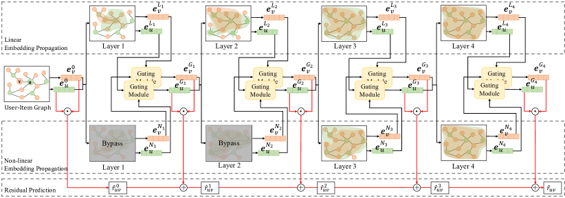
Figure 2. The detailed workflow of HMLET(End). One can consider our gating module as a relay switch between the linear and non-linear propagation. While calculating an embedding for a user or an item in the third and fourth layer, therefore, our gating module learns the optimal selection between them for each node. For instance, it can select a sequence of linear $\rightarrow$ linear $\rightarrow$ linear $\rightarrow$ non-linear for some nodes while it can select a totally different sequence for other nodes.

We first formulate our problem of top-$N$ recommendation as follows: Let $u\in U$ and $v\in I$ denote a user and an item, respectively, where $U$ and $I$ denote the sets of all users and all items, respectively; $N_{u}$ denotes a set of items rated by user $u$. For each user $u$, the goal is to recommend the top-$N$ items that are most likely to be preferred by $u$ among her unrated items,  $I\setminus N_{u}$.

In this section, among several variations of , we mainly describe HMLET(End) for ease of writing because it shows the best accuracy — other variations can be easily modified from HMLET(End) and we omit their descriptions. Its key concept is to adopt the gating between the linear and non-linear propagation in a layer. In other words, we prepare both the linear and non-linear propagation steps in a layer and let our gating module with STGS decide which one to use for each node. Table 3 summarizes a list of notations used in this paper.

Figure 2 illustrates the overall workflow of HMLET(End). After constructing the user-item interaction as a user-item bipartite graph,  initializes the user and item embeddings in the initialization step. After that, each embedding is propagated to its neighbors through $K$ propagation layers. The gating module in  selects either of the linear or the non-linear propagation in a layer for each node (Section 3.1). To this end, we use the gating module with STGS. In order to predict each user’s preference on each item, the dot product of the user embedding and the item embedding in each layer is aggregated and we use their sum for prediction (Section 3.2).

Table 3. Notations used in this paper

Notation	Description
$K$	The number of total layers
$\bm{e}_{u}^{L_{i}}$, $\bm{e}_{v}^{L_{i}}$	$u$’s and $v$’s embeddings at $i$-th linear layer
$\bm{e}_{u}^{N_{i}}$, $\bm{e}_{v}^{N_{i}}$	$u$’s and $v$’s embeddings at $i$-th non-linear layer
$\bm{e}_{u}^{G_{i}}$, $\bm{e}_{v}^{G_{i}}$	$u$’s and $v$’s embeddings selected by the gating module at $i$-th layer
$D$	The size (dimension) of embedding
$|U|$, $|I|$	The number of users and items
$\hat{r}_{uv}$	The user $u$’s final preference on item $v$
$\mathcal{N}_{u}$, $\mathcal{N}_{v}$	The set of items rated to user $u$ and the set of users who rated item $v$

3.1. Propagation Layer

We omit the description of the initialization step due to its obviousness.  propagates the embedding $\bm{e}_{u}$ (resp. $\bm{e}_{v}$) of each user $u$ (resp. each item $v$) through the propagation layers. In this subsection, we describe the propagation process. We first formally define the linear and the non-linear propagation steps used in this paper. Then, we present our gating module.

3.1.1. Propagation

Recently, the authors of LightGCN (He et al., 2020a) found that the feature transformation and the non-linear activation do not have a positive effect on the effectiveness of CF. So, LightGCN removed the feature transformation and the non-linear activation from Eq. (1), and it shows better performance than existing non-linear GCNs for recommendation. In , we adopt the linear layer definition of LightGCN. Therefore, our linear embedding propagation is performed as follows:

(4) $$\begin{split}\bm{e}_{u}^{L_{i+1}}=\mathop{{\sum}}_{v\in\mathcal{N}_{u}}\frac{1}{\sqrt{|\mathcal{N}_{u}\|\mathcal{N}_{v}|}}\bm{e}_{v}^{G_{i}},\;\;\;\bm{e}_{v}^{L_{i+1}}=\mathop{{\sum}}_{u\in\mathcal{N}_{v}}\frac{1}{\sqrt{|\mathcal{N}_{u}\|\mathcal{N}_{v}|}}\bm{e}_{u}^{G_{i}},\end{split}$$

where $\bm{e}_{u}^{L_{i+1}}$ and $\bm{e}_{v}^{L_{i+1}}$ are the linear embeddings for user $u$ and item $v$. Since our gating module, which will be described shortly, selects between the linear and the non-linear embeddings, $\bm{e}_{u}^{G_{i}}$ and $\bm{e}_{v}^{G_{i}}$ means the embeddings selected by our gating module in the previous $i$-th layer. If $i=0$, $\bm{e}_{u}^{G_{i}}=\bm{e}_{u}^{0}$ and $\bm{e}_{v}^{G_{i}}=\bm{e}_{v}^{0}$,   initial embeddings. $\frac{1}{\sqrt{|\mathcal{N}_{u}\|\mathcal{N}_{v}|}}$ is a symmetric normalization term to restrict the scale of embeddings into a reasonable boundary.

For the non-linear embedding propagation, we design a variant of the linear embedding propagation by adding non-linear activation functions. Its propagation is preformed as follows:

(5) $$\begin{split}\bm{e}_{u}^{N_{i+1}}=\left\{\begin{array}[]{ll}\bm{e}_{u}^{N_{i}},&\text{if~{}}bypass\\ \phi\Big{(}\mathop{{\sum}}_{v\in\mathcal{N}_{u}}\frac{1}{\sqrt{|\mathcal{N}_{u}\|\mathcal{N}_{v}|}}\bm{e}_{v}^{G_{i}}\Big{)},&\text{if~{}}propagate,\end{array}\right.\\ \bm{e}_{v}^{N_{i+1}}=\left\{\begin{array}[]{ll}\bm{e}_{v}^{N_{i}},&\text{if~{}}bypass\\ \phi\Big{(}\mathop{{\sum}}_{u\in\mathcal{N}_{v}}\frac{1}{\sqrt{|\mathcal{N}_{u}\|\mathcal{N}_{v}|}}\bm{e}_{u}^{G_{i}}\Big{)},&\text{if~{}}propagate,\end{array}\right.\\ \end{split}$$

where $\phi$ is a non-linear activation function, e.g., ELU, Leaky ReLU. For instance, as shown in Figure 2, HMLET(End) bypasses the non-linearity propagation on the first and second layers to address the over-smoothing problem and then propagates the non-linear embedding in the third and fourth layers.

3.1.2. Gating Module

Now, we have the two types of the embeddings for each node, created by the linear and non-linear propagation in Eqs. (4) and (5), respectively, in the previous $i\text{-th}$ layer. Therefore, we should select one of the linear and non-linear embeddings for the propagation in the next $(i+1)\text{-th}$ layer.

Toward this end, we add a gating module, which dynamically selects either of the linear or non-linear embedding after understanding the inherent characteristics of nodes. A separate gating module should be added whenever the linear and the non-linear propagation co-exist in a layer. The intuition behind this technique is that i) the embeddings of nodes may exhibit both the linearity and the non-linearity in their characteristics and ii) the linearity and the non-linearity of nodes may vary from one layer to another.

The process of the gating module with STGS is shown in Algorithm  1. For simplicity but without loss of generality, we use the symbol $\bm{e}^{L}$ and $\bm{e}^{N}$ to denote the linear and non-linear embeddings, respectively, after omitting other subscripts and superscripts. We support three gating types: i) choose the linear embedding (bypassing the non-linear propagation), ii) choose the non-linear embedding (bypassing the linear propagation), and iii) let the gating module choose one of them. The variable $\xi$ notates the gating type. If $\xi$ is the first or second type, a designated embedding type is selected. If $\xi$ is the third type, the input embeddings,  the linear and non-linear embedding, are concatenated and then passed to an MLP (multi-layer perceptron) (Lines 7 and 8 in Algorithm 1). The result of the MLP is a logit vector $\bm{l}$, an input for STGS (Line 9). The logit vector $\bm{l}$ corresponds to $\log\bm{\pi}$ explained in Section 2.2. $\bm{g}$ represents a linear or non-linear selection by the gating module,   $\bm{g}$ is a two-dimensional one-hot vector. Therefore, $\bm{e}^{G}$ is the same as either of $\bm{e}^{L}$ or $\bm{e}^{N}$ (Line 10).

Input: Linear embedding $\bm{e}^{L}$, Non-linear embedding $\bm{e}^{N}$, Temperature $\tau$, Gating type $\xi$

1 Function Gating_Module($\bm{e}^{L},\bm{e}^{N},\tau$, $\xi$):

2       if $\xi$ = linear then

3             $\bm{e}^{G}\leftarrow\bm{e}^{L}$

4            

5       else if $\xi$ = non-linear then

6             $\bm{e}^{G}\leftarrow\bm{e}^{N}$

7            

8       else

9             $\bm{e}_{\text{concat}}\leftarrow\bm{e}^{L}||\bm{e}^{N}$

10             $\bm{l}\leftarrow\text{MLP}(\bm{e}_{\text{concat}})$

11             $\bm{g}\leftarrow\text{STGS}(\bm{l},\tau)$

12             $\bm{e}^{G}\leftarrow\bm{g}\cdot[\bm{e}^{L},\bm{e}^{N}]$

13            

14      return $\bm{e}^{G}$

15      

Algorithm 1 Gating Module

3.1.3. Variants of HMLET

As shown in Figure 1 and Table 4, there can be four variants of , denoted as HMLET(All), HMLET(Front), HMLET(Middle), and HMLET(End), depending on the locations of the non-linear layers. Each method except HMLET(All) uses up to 2 non-linear layers since it is known that more than 2 non-linear layers cause the problem of over-smoothing (Chen et al., 2020b). Moreover, we test with various options of where to put them. First, HMLET(Front) focuses on the fact that GCNs are highly influenced by close neighborhood,  in the first and second layers (Tang et al., 2015). Therefore, HMLET(Front) adopts the gating module in the front and uses only the linear propagation layers afterwards. Second, HMLET(Middle) only uses the linear propagation in the front and last and then adopts the gating module in the second and third layers. Last, as the gating module is located in the third and fourth layers, HMLET(End) focuses on gating in the third and fourth layers — our experiments and analyses show that HMLET(End) is the best among the four variations of the proposed method. We select $\bm{e}^{L_{3}}$ or $\bm{e}^{N_{3}}$ at the third layer and $\bm{e}^{L_{4}}$ or $\bm{e}^{N_{4}}$ at the fourth layer via the gating modules, respectively. If the linear embeddings are selected for a node in all layers, it is the same as using a linear GCN with $K=4$ for processing the node. If the non-linear embedding is selected for other node in all layers, it reduces to a non-linear GCN with $K=2$. Likewise, HMLET(End) can be considered as a node-wise dynamic GCN (between the linear and non-linear propagation) with varying $K\in\{2,4\}$.

Table 4. Variants of  in terms of their setting for the non-linear propagation in Eq. (5) and the gating type $\xi$

Layer	1	2	3	4
HMLET(All)	propagate/gating	propagate/gating	propagate/gating	propagate/gating
HMLET(Front)	propagate/gating	propagate/gating	bypass/linear	bypass/linear
HMLET(Middle)	bypass/linear	propagate/gating	propagate/gating	bypass/linear
HMLET(End)	bypass/linear	bypass/linear	propagate/gating	propagate/gating

Input: The number of total layers $K$, A bipartite graph $G$

1 Function ($K,G$):

2      Initialize $\bm{e}_{u}^{0},\bm{e}_{v}^{0},~{}\text{for}~{}\forall u,~{}\forall v$

3      $iter\leftarrow 0$

4      while the BPR loss is not converged do

5           $\tau\leftarrow 1.0\exp(-0.001\times iter)$

6           $\hat{r}_{u,v}\mathrel{{=}}\bm{e}_{u}^{0}\odot\ \bm{e}_{v}^{0},~{}\text{for}~{}\forall u,~{}\forall v$

7           for $i\leftarrow 1\;\text{to}\;K$ do

8                $\bm{e}_{u}^{L_{i}},\bm{e}_{v}^{L_{i}}=\text{Eq}.~{}\eqref{eq:linear},~{}\text{for}~{}\forall u,~{}\forall v$

9                $\bm{e}_{u}^{N_{i}},\bm{e}_{v}^{N_{i}}=\text{Eq}.~{}\eqref{eq:non-linear},~{}\text{for}~{}\forall u,~{}\forall v$

10                $\bm{e}_{u}^{G_{i}}=\textnormal{{Gating\_Module}}(\bm{e}_{u}^{L_{i}},\bm{e}_{u}^{N_{i}},\tau,\xi_{i}),~{}\text{for}~{}\forall u$

11                $\bm{e}_{v}^{G_{i}}=\textnormal{{Gating\_Module}}(\bm{e}_{v}^{L_{i}},\bm{e}_{v}^{N_{i}},\tau,\xi_{i}),~{}\text{for}~{}\forall v$

12                $\hat{r}_{u,v}\mathrel{{+}{=}}\bm{e}_{u}^{G_{i}}\odot\bm{e}_{v}^{G_{i}},~{}\text{for}~{}\forall u,~{}\forall v$

13               

14          Update $\bm{e}_{u}^{0},\bm{e}_{v}^{0}$ with the BPR Loss for $\forall u,\forall v$

15           Train the parameters of the gating modules with the BPR Loss

16           $iter\mathrel{{+}{=}}1$

17          

18     return $\hat{r}_{u,v}$, for $\forall u,\forall v$

19     

Algorithm 2

3.2. Prediction Layer

After propagating through all $K$ layers, we predict a user $u$’s preference for an item $v$. To this end, we create a dot product value of $\bm{e}^{G_{i}}_{u}$ and $\bm{e}^{G_{i}}_{v}$ in each layer and use the following residual prediction:

(6) $$\begin{gathered}\hat{r}^{i}_{uv}=\bm{e}_{u}^{G_{i}}\odot\bm{e}_{v}^{G_{i}},\;\;\;\hat{r}_{uv}=\;\beta\mathop{{\sum}}^{K}_{i=0}\hat{r}^{i}_{uv}.\end{gathered}$$

In some layers, a gating module can be missing. In such a case, there is only one type of embeddings, but we also use $\bm{e}_{u}^{G_{i}}$/$\bm{e}_{v}^{G_{i}}$ to denote these embeddings for ease of writing.

In most previous GCN-based recommender system research, only the embedding of the last layer was used to predict, but in , the above residual prediction $\hat{r}_{uv}$ with $\beta$ is used. Similar to LightGCN, $\beta$ is set to $1/(K+1)$. This residual prediction can produce good performance by using not only the embedding in the last layer but also the embeddings in previous layers.

3.3. Training Method

For training , we employ the Bayesian Personalized Ranking (BPR) loss (Rendle et al., 2009), denoted $\bm{L}$, which is frequently used in many CF methods. The BPR loss is written as follows:

(7) $$\begin{split}\bm{L}=-\mathop{{\sum}}^{|U|}_{u=1}\mathop{{\sum}}_{i\in N_{u}}\mathop{{\sum}}_{j\notin N_{u}}\ln(\sigma(\hat{r}_{ui}-\hat{r}_{uj}))+\lambda\lVert\bm{\Theta}\rVert^{2},\end{split}$$

where $\sigma$ is the sigmoid function. $\bf{\Theta}$ is the initial embeddings and the parameters of the gating modules, and $\lambda$ controls the $L_{2}$ regularization strength. We use each observed user-item interaction as a positive instance and employ the strategy used in (He et al., 2020a) for sampling a negative instance.

We employ STGS for a smooth optimization of the gating module. We can train the network with annealing the temperature $\tau$, and we use the temperature decay for each epoch (Line 2 in Algorithm 2). In order to calculate $\hat{r}_{uv}$ as in Eq. (6), we accumulate the dot product results (Lines 2 and 2). Then, we train the initial embeddings (Line 2) and the parameters of the gating modules (Line 2).

4. Experiments

In this section, we evaluate our proposed approach via comprehensive experiments. We design our experiments, aiming at answering the following key research questions (RQs):

• RQ1: Which variation of is the most effective in terms of recommendation accuracy?

• RQ2: Does gating between the linear and non-linear propagation provide more accurate recommendations than baseline methods?

• RQ3: What are the characteristics of the nodes that use i) only the linear propagation, ii) only the non-linear propagation, or iii) different propagation steps in different layers?

4.1. Experimental Environments

4.1.1. Datasets

For evaluation, we used the following three real-word datasets: Gowalla, Yelp2018, and Amazon-Book from various domains. They are all publicly available. Table 5 shows the detailed statistics of the three datasets.

• Gowalla is a location-based social networking website where users share their locations by checking-in (Liang et al., 2016). This dataset contains user-website interactions.

• Yelp2018 is a subset of small business and user data used in Yelp Dataset Challenge 2018. This dataset contains user-business interactions.

• Amazon-Book contains purchase records of Amazon users (He and McAuley, 2016). This dataset contains user-item interactions. Amazon-Book has the highest sparsity among these three public datasets.

Table 5. Statistics of public benchmark datasets

Dataset	# User	# Item	# Interaction	Sparsity
Gowalla	29,858	40,981	1,027,370	99.916%
Yelp2018	31,668	38,048	1,561,406	99.870%
Amazon-Book	52,643	91,599	2,984,108	99.938%

Following (Wang et al., 2019), we filtered out those users and items with less than ten interactions in all datasets,  a 10-core setting. For testing, we then split a dataset into training (80%), validation (10%), and test (10%) sets in the same way as in  (Wang et al., 2019).

4.1.2. Baseline Methods

We compare with the following five state-of-the-art methods to verify its effectiveness:

• BPR (Rendle et al., 2009) is a matrix factorization (MF) trained by the Bayesian Personalized Ranking (BPR) loss.

• WRMF (Hu et al., 2008) is an MF solved by the weight alternating least square (WALS) technique.

• NGCF (Wang et al., 2019) is a non-linear GCN-based recommender system performing residual prediction.

• LR-GCCF (Chen et al., 2020b) is a linear GCN-based recommender system which removes the non-linear activation function but still use the transformation matrix in Eq. (1). This method performs the residual prediction.

• LightGCN (He et al., 2020a) is yet another linear GCN-based recommender system performing the residual prediction. This method differs from LR-GCCF in that it does not use the transformation matrix.

For MF-based methods, we use the implementations in the popular open-source library, called NeuRec. For GCN-based methods, we use the source codes provided by the authors (He et al., 2020a; Chen et al., 2020b; Wang et al., 2019). To evaluate accuracy, we use the top-20 recommendations and measure the accuracy in terms of the normalized discounted cumulative gain (NDCG), recall, and precision, which are all frequently used in recommendation research (Wang et al., 2019; Chen et al., 2020b; He et al., 2020a).

4.1.3. Hyper-parameter Settings

We choose the best hyper-parameter set via the grid search with the validation set. The best setting found in is as follows: the number of linear layers is set to 4; the number of non-linear layers is set to 4 in HMLET(All) and 2 for HMLET(Front), HMLET(Middle), and HMLET(End); the optimizer is Adam; the learning rate is 0.001; the $L_{2}$ regularization coefficient $\lambda$ is 1E-4; the mini-batch size is 2,048; the dropout rate is 0.4. And, we use the temperature $\tau$ with an initialization to 0.7, a minimum temperature of 0.01, and a decay factor of 0.995. Also, for fair comparison, we set the embedding sizes for all methods to 512. In non-linear layers, we test two non-linear activation functions: Leaky-ReLU (negative slope = 0.01) and ELU ($\alpha$ = 1.0). For baseline models, we tuned their hyper-parameters via the grid search in the ranges suggested in their respective papers.

4.2. Experimental Results

Figure 3. The comparison of NDCG@20 with all types of in three public benchmarks.

4.2.1. Comparison among Model Variations (RQ1)

For answering RQ1, we first compare the accuracies of HMLET(All), HMLET(Front), HMLET(Middle), and HMLET(End). Figures 3 illustrates the results where X-axis represents the types of , and Y-axis represents NDCG@20.

Table 6. The comparison of overall performance with baseline models on three public benchmarks

	Amazon-Book			Yelp2018			Gowalla
Metrics	NDCG@20	Recall@20	Precision@20	NDCG@20	Recall@20	Precision@20	NDCG@20	Recall@20	Precision@20
BPR	0.0181	0.0307	0.0065	0.0289	0.0476	0.0062	0.0847	0.1341	0.0203
WRMF	0.0242	0.0405	0.0085	0.0402	0.0645	0.0145	0.1007	0.1538	0.0243
NGCF	0.0250	0.0426	0.0086	0.0371	0.0601	0.0134	0.1071	0.1661	0.0253
LR-GCCF	0.0213	0.0361	0.0077	0.0351	0.0581	0.0129	0.0989	0.1545	0.0240
LightGCN	0.0283	0.0484	0.0099	0.0420	0.0678	0.0152	0.1212	0.1870	0.0288
HMLET(End)	0.0300	0.0510	0.0103	0.0434	0.0696	0.0155	0.1231	0.1908	0.0293
%Improve	6.00%	5.37%	4.04%	3.33%	2.65%	1.97%	1.56%	2.03%	1.73%
$p$-value	1.59E-37	1.71E-34	5.16E-36	5.57E-58	2.90E-39	1.61E-44	8.51E-25	4.17E-131	3.39E-27

Table 7. The selection ratio by gating modules in Amazon-Book

	Layer 1		Layer 2		Layer 3		Layer 4
Propagation	Linear	Non-Lin.	Linear	Non-Lin.	Linear	Non-Lin.	Linear	Non-Lin.
HMLET(All)	77.05%	22.95%	60.45%	39.55%	68.01%	31.99%	40.77%	59.23%
HMLET(Front)	74.30%	25.70%	62.09%	37.91%	100%	0%	100%	0%
HMLET(Middle)	100%	0%	63.03%	36.97%	72.41%	27.59%	100%	0%
HMLET(End)	100%	0%	100%	0%	5.19%	94.81%	49.55%	50.45%

HMLET(End) is the best among all variations of . The accuracies of all variations except HMLET(End) are similar. Specifically, the difference between HMLET(End) and other variations is around 7%, 0.9%, 1% in Amazon-Book, Yelp2018, and Gowalla, respectively. However, the differences in accuracy among HMLET(All), HMLET(Front), and HMLET(Middle) are as small as 0.2%.

These results indicate that i) the effectiveness of the gating module greatly depends on the location where the gating module exists, and ii) the non-linear propagation is useful to capture distant neighborhood information — note that we added the gating modules at the last two layers in HMLET(End). As shown in Table 7, each variation has a quite different linear/non-linear embedding selection ratio. HMLET(End), the best model, uses the non-linear propagation in the layers 3 and 4, and their selection ratios are significant, e.g.,  5.19% of linear vs. 94.81% of non-linear in the third layer. This observation also applies to the second best model, HMLET(All). Similar selection ratio patterns are observed in the other two datasets.

4.2.2. Comparison with Baselines (RQ2)

Table 6 illustrates our main experimental results. In them, the values in boldface indicate the best accuracy in each column, and the values in italic mean the best baseline accuracy. Also, ‘%Improve’ indicates the degree of accuracy improvements over the best baseline by HMLET(End). Lastly, we conduct $t$-tests with a 95% confidence level to verify the statistical significance of the accuracy differences between HMLET(End) and the baselines.

We summarize the results shown in Table 6 as follows. First, among the five baseline methods, we observe that LightGCN consistently shows the best accuracy in all datasets. Second, HMLET(End) consistently provides the highest accuracy in all datasets and with all metrics. Specifically, HMLET(End) outperforms LightGCN by 6.00%, 3.33%, and 1.56% for the datasets in terms of NDCG@20, respectively. The $p$-values are below $0.05$, indicating that the differences are statistically significant. We highlight that HMLET(End) shows remarkable improvements in Amazon-Book which is the largest dataset in this paper.

4.3. Linearity or Non-Linearity

In this subsection, we define three different classes of nodes, depending on their preferences on the linear or non-linear propagation, and perform in-depth analyses on them. In order to analyze accurately, we use the embeddings learned by HMLET(End), the best performing variation of , for Amazon-Book. Due to space limitations, we omit the results for the other datasets, which show similar patterns to those in Amazon-Book.

4.3.1. Node Class and Graph Centrality

We first classify all nodes into one of the following three classes according to the embedding types selected by the gating modules:

• Full-Non-Linearity (FNL) is a class of nodes in which all embeddings selected by the gating modules are non-linear embeddings.

• Partial-Non-Linearity (PNL) is a class of nodes in which the embeddings selected by the gating modules are mixed with linear embeddings and non-linear embeddings.

• Full-Linearity (FL) is a class of nodes in which all embeddings selected by the gating modules are linear embeddings.

We next introduce three graph centrality metrics to study the characteristics of the classes:

• PageRank  (Page et al., 1999) measures the relative importance of nodes in a graph. A node is considered as important, even though its connectivity with other nodes is not that strong, if connected to other important nodes.

• Betweenness Centrality  (Brandes, 2001) measures the centrality of a node as an intermediary in a graph. The more a node appears in multiple shortest paths, the higher the betweenness centrality of the node.

• Closeness Centrality (Freeman, 1978) measures the centrality of a node by considering general connections to other nodes in a graph. The less hops it takes for a node to reach all other nodes, the higher the closeness centrality.

4.3.2. Characteristics of Node Classes (RQ3)

In this subsection, we analyze the characteristics of the nodes in each class in terms of the various centrality metrics. Table 8 shows the relative class size in our three datasets. In Amazon-Book and Yelp2018, most nodes were classified as FNL and PNL (about 47-48% and 50-52%, respectively), and a few nodes were classified as FL (about 1-2%). However, in Gowalla, the ratio of FL is about 12%, which is relatively higher compared to the other two datasets. Figure 4 shows the relative sizes of the three classes by degree, and Figure 5 shows the statistics of the centrality scores in each class. From them, it can be seen that the degree and centrality scores increase in order of FL, PNL, and FNL. Now, we deliver the meaning of the above results for each class.

Table 8. The relative class sizes in three datasets

Class	Amazon-Book	Yelp2018	Gowalla
FNL	46.78%	47.95%	27.49%
PNL	51.77%	49.59%	60.84%
FL	1.45%	2.46%	11.67%

Figure 4. The class ratio of nodes sorted by degree. $i$-th bin in X-axis means a range of [$(10*(i-1))$-th percentile, $(10*i)$-th percentile) in terms of degree. Nodes with a high degree are the most likely to be in FNL (10th), and nodes with a small degree are likely to be in FL (1st). We also find that nodes classified as PNL are more evenly distributed than other classes.

• FNL Attributes: A node in FNL is either an active user or a popular item with more direct/indirect interaction information,  a high degree and closeness centrality, and higher influence,  a high PageRank and betweenness centrality, than nodes in other classes. So, they will receive a lot of information during the propagation step. Therefore, the sophisticated non-linear propagation is required to correctly extract useful information from much potentially noisy information.

• FL Attributes: A node in FL is either a user or an item that does not have much direct/indirect interaction information,  a low degree and closeness centrality, and little influence,  a low PageRank and betweenness centrality, compared to nodes in other classes. The information they receive during the propagation step may mostly consist of useful information related to themselves with little noise. Therefore, the simple linear propagation is required to take useful information as it is, rather than refining it.

• PNL Attributes: A node in PNL, compared to nodes in other classes, is a user or an item with neither too large nor too small direct/indirect interaction information,  a moderate degree and closeness centrality, and influence,  a moderate PageRank and betweenness centrality. In other words, although they have many direct neighbors, there are few indirect neighbors connected to the direct neighbors, or even if there are few direct neighbors, their indirect neighbors can be many. Therefore, they need to perform one of the non-linear or linear operations depending on the information they receive from neighbors.

Figure 5. The statistics of PageRank, betweenness centrality, and closeness centrality.

In order to double-check our interpretations, we show the statistics of the similarity of embeddings for each class. So, we calculate the cosine similarity between a node and its direct neighbors by using the embeddings learned by HMLET(End). The results are shown in Table 9. From these results, we can confirm that the neighbors of a node in FNL consist of diversified nodes,  a low mean and high variance. Also, FL nodes’ neighbors mainly consist of similar nodes,  a high mean and low variance. Lastly, PNL nodes’ neighbors are in between the previous two cases,  a moderate mean and variance between nodes in other classes.

Table 9. The statistics of the cosine similarity between a node’s embedding and its direct neighbors’ embeddings in each node class

Similarity	FNL	PNL	FL
Mean	0.6369	0.6449	0.7157
Variance	0.0179	0.0162	0.0160

5. Conclusions and Future Work

In this paper, we presented a novel GCN-based CF method, named as , that can select the linear or non-linear propagation step in a layer for each node. We further analyzed how the linear/non-linear selection mechanism works using various graph analytics techniques. To this end, we first designed our linear and non-linear propagation steps, being inspired by various state-of-the-art linear and non-linear GCNs for CF. Then, we used STGS to learn the optimal selection between the linear and non-linear propagation steps. The intuition behind such design choice is that it is not optimal to put both the linear and the non-linear propagation in every layer. In this sense, we have defined several variations of  in terms of combining the linear and non-linear propagation steps.

Through extensive experiments using three standard benchmark datasets, we demonstrated that  shows the best accuracy in all datasets. Furthermore, we presented in-depth analyses of how the linearity and non-linearity of nodes are decided in a graph. Toward this end, we classified nodes into three classes,  Full-Non-Linearity, Partial-Non-Linearity, and Full-Linearity, depending on our gating module’s selections and studied correlations between nodes’ centrality scores and their class membership.

We conjecture that GCNs for CF should somehow consider both linear and non-linear operations. We do not say that our specific mechanism to combine the linear and the non-linear propagation steps is optimal. We hope that our discovery encourages much follow-up research work.

References

- (1)
- Brandes (2001) Ulrik Brandes. 2001. A faster algorithm for betweenness centrality. Journal of mathematical sociology 25, 2 (2001), 163–177.
- Bruna et al. (2014) Joan Bruna, Wojciech Zaremba, Arthur Szlam, and Yann LeCun. 2014. Spectral networks and deep locally connected networks on graphs. In Proc. of the Int’l Conf. on Learning Representations (ICLR).
- Chae et al. (2018) Dong-Kyu Chae, Jin-Soo Kang, Sang-Wook Kim, and Jung-Tae Lee. 2018. CFGAN: A Generic Collaborative Filtering Framework based on Generative Adversarial Networks. In Proc. of the ACM Int’l Conf. on Information and Knowledge Management (CIKM).
- Chae et al. (2020) Dong-Kyu Chae, Jihoo Kim, Duen Horng Chau, and Sang-Wook Kim. 2020. AR-CF: Augmenting Virtual Users and Items in Collaborative Filtering for Addressing Cold-Start Problems. In Proc. of the ACM Int’l Conf. on Research & Development in Information Retrieval (SIGIR).
- Chen et al. (2020a) Deli Chen, Yankai Lin, Wei Li, Peng Li, Jie Zhou, and Xu Sun. 2020a. Measuring and relieving the over-smoothing problem for graph neural networks from the topological view. In Proc. of the AAAI Conf. on Artificial Intelligence (AAAI).
- Chen et al. (2020b) Lei Chen, Le Wu, Richang Hong, Kun Zhang, and Meng Wang. 2020b. Revisiting Graph Based Collaborative Filtering: A Linear Residual Graph Convolutional Network Approach. In Proc. of the AAAI Conf. on Artificial Intelligence (AAAI).
- Choi et al. (2021) Jeongwhan Choi, Jinsung Jeon, and Noseong Park. 2021. LT-OCF: Learnable-Time ODE-based Collaborative Filtering. In Proc. of the ACM Int’l Conf. on Information and Knowledge Management (CIKM).
- Ebesu et al. (2018) Travis Ebesu, Bin Shen, and Yi Fang. 2018. Collaborative Memory Network for Recommendation Systems. In Proc. of the ACM Int’l Conf. on Research & Development in Information Retrieval (SIGIR).
- Freeman (1978) Linton C Freeman. 1978. Centrality in social networks conceptual clarification. Social networks 1, 3 (1978), 215–239.
- Goodfellow et al. (2014) Ian Goodfellow, Jean Pouget-Abadie, Mehdi Mirza, Bing Xu, David Warde-Farley, Sherjil Ozair, Aaron Courville, and Yoshua Bengio. 2014. Generative adversarial nets. In Proc. of the Annual Conf. on Neural Information Processing Systems (NeurIPS).
- Gumbel (1954) Emil Julius Gumbel. 1954. Statistical theory of extreme values and some practical applications. NBS Applied Mathematics Series 33 (1954).
- Hamilton et al. (2017) William L. Hamilton, Rex Ying, and Jure Leskovec. 2017. Inductive Representation Learning on Large Graphs. In Proc. of the Annual Conf. on Neural Information Processing Systems (NeurIPS).
- He et al. (2020b) Chaoyang He, Haishan Ye, Li Shen, and Tong Zhang. 2020b. Milenas: Efficient neural architecture search via mixed-level reformulation. In Proc. of the IEEE/CVF Conf. on Computer Vision and Pattern Recognition (CVPR).
- He and McAuley (2016) Ruining He and Julian McAuley. 2016. Ups and downs: Modeling the visual evolution of fashion trends with one-class collaborative filtering. In Proc. of The Web Conference (WWW).
- He et al. (2020a) Xiangnan He, Kuan Deng, Xiang Wang, Yan Li, YongDong Zhang, and Meng Wang. 2020a. LightGCN: Simplifying and Powering Graph Convolution Network for Recommendation. In Proc. of the ACM Int’l Conf. on Research & Development in Information Retrieval (SIGIR).
- He et al. (2017) Xiangnan He, Lizi Liao, Hanwang Zhang, Liqiang Nie, Xia Hu, and Tat-seng Chua. 2017. Neural Collaborative Filtering. In Proc. of The Web Conference (WWW).
- Hu et al. (2020) Shoukang Hu, Sirui Xie, Hehui Zheng, Chunxiao Liu, Jianping Shi, Xunying Liu, and Dahua Lin. 2020. Dsnas: Direct neural architecture search without parameter retraining. In Proc. of the IEEE/CVF Conf. on Computer Vision and Pattern Recognition (CVPR).
- Hu et al. (2008) Yifan Hu, Yehuda Koren, and Chris Volinsky. 2008. Collaborative filtering for implicit feedback datasets. In Proc. of the IEEE Int’l Conf. on Data Mining (ICDM).
- Hwang et al. (2016) Won-Seok Hwang, Juan Parc, Sang-Wook Kim, Jongwuk Lee, and Dongwon Lee. 2016. ”Told you i didn’t like it”: Exploiting uninteresting items for effective collaborative filtering. In Proc. of the IEEE Int’l Conf. on Data Engineering (ICDE).
- Jang et al. (2016) Eric Jang, Shixiang Gu, and Ben Poole. 2016. Categorical reparameterization with gumbel-softmax. In Proc. of the Int’l Conf. on Learning Representations (ICLR).
- Kingma and Welling (2013) Diederik P Kingma and Max Welling. 2013. Auto-encoding variational bayes. arXiv preprint arXiv:1312.6114 (2013).
- Kipf and Welling (2017) Thomas N. Kipf and Max Welling. 2017. Semi-Supervised Classification with Graph Convolutional Networks. In Proc. of the Int’l Conf. on Learning Representations (ICLR).
- Koren et al. (2009) Y. Koren, R. Bell, and C. Volinsky. 2009. Matrix Factorization Techniques for Recommender Systems. Computer 42, 8 (2009), 30–37.
- Lee et al. (2018) Yeon-Chang Lee, Sang-Wook Kim, and Dongwon Lee. 2018. gOCCF: Graph-Theoretic One-Class Collaborative Filtering Based on Uninteresting Items. In Proc. of the AAAI Conf. on Artificial Intelligence (AAAI).
- Li et al. (2020) Yanxi Li, Minjing Dong, Yunhe Wang, and Chang Xu. 2020. Neural architecture search in a proxy validation loss landscape. In Proc. of the Int’l Conf. on Machine Learning (ICML).
- Liang et al. (2016) Dawen Liang, Laurent Charlin, James McInerney, and David M Blei. 2016. Modeling user exposure in recommendation. In Proc. of The Web Conference (WWW).
- Maddison et al. (2014) Chris J Maddison, Daniel Tarlow, and Tom Minka. 2014. A* sampling. arXiv preprint arXiv:1411.0030 (2014).
- Page et al. (1999) Lawrence Page, Sergey Brin, Rajeev Motwani, and Terry Winograd. 1999. The PageRank citation ranking: Bringing order to the web. Technical Report. Stanford InfoLab.
- Park et al. (2018) David Keetae Park, Seungjoo Yoo, Hyojin Bahng, Jaegul Choo, and Noseong Park. 2018. MEGAN: Mixture of Experts of Generative Adversarial Networks for Multimodal Image Generation. In Proc. of the Int’l Joint Conf. on Artificial Intelligence (IJCAI).
- Rendle et al. (2009) Steffen Rendle, Christoph Freudenthaler, Zeno Gantner, and Lars Schmidt-Thieme. 2009. BPR: Bayesian Personalized Ranking from Implicit Feedback. In Proc. of the Int’l Conf. on Uncertainty in Artificial Intelligence (UAI).
- Tang et al. (2015) Jian Tang, Meng Qu, Mingzhe Wang, Ming Zhang, Jun Yan, and Qiaozhu Mei. 2015. Line: Large-scale information network embedding. In Proc. of The Web Conference (WWW).
- van den Berg et al. (2018) Rianne van den Berg, Thomas N. Kipf, and Max Welling. 2018. Graph Convolutional Matrix Completion. In Proc. of the ACM Int’l Conf. on Knowledge Discovery and Data Mining (KDD).
- Vincent et al. (2008) Pascal Vincent, Hugo Larochelle, Yoshua Bengio, and Pierre-Antoine Manzagol. 2008. Extracting and composing robust features with denoising autoencoders. In Proc. of the Int’l Conf. on Machine Learning (ICML).
- Wang et al. (2014) Hao Wang, Naiyan Wang, and Dit-Yan Yeung. 2014. Collaborative Deep Learning for Recommender Systems. In Proc. of the ACM Int’l Conf. on Knowledge Discovery and Data Mining (KDD).
- Wang et al. (2019) Xiang Wang, Xiangnan He, Meng Wang, Fuli Feng, and Tat-Seng Chua. 2019. Neural Graph Collaborative Filtering. In Proc. of the ACM Int’l Conf. on Research & Development in Information Retrieval (SIGIR).
- Wu et al. (2019a) Bichen Wu, Xiaoliang Dai, Peizhao Zhang, Yanghan Wang, Fei Sun, Yiming Wu, Yuandong Tian, Peter Vajda, Yangqing Jia, and Kurt Keutzer. 2019a. Fbnet: Hardware-aware efficient convnet design via differentiable neural architecture search. In Proc. of the IEEE/CVF Conf. on Computer Vision and Pattern Recognition (CVPR).
- Wu et al. (2019b) Felix Wu, Tianyi Zhang, Amauri Holanda de Souza, Christopher Fifty, Tao Yu, and Kilian Q. Weinberger. 2019b. Simplifying Graph Convolutional Networks. In Proc. of the Int’l Conf. on Machine Learning (ICML).
- Ying et al. (2018) Rex Ying, Ruining He, Kaifeng Chen, Pong Eksombatchai, William L. Hamilton, and Jure Leskovec. 2018. Graph Convolutional Neural Networks for Web-Scale Recommender Systems. In Proc. of the ACM Int’l Conf. on Knowledge Discovery and Data Mining (KDD).
- Zhang et al. (2020) Guijuan Zhang, Yang Liu, and Xiaoning Jin. 2020. A survey of autoencoder-based recommender systems. Frontiers of Computer Science 14, 2 (2020), 430–450.