Cosmic Shear in Harmonic Space from the Dark Energy Survey Year 1 Data: Compatibility with Configuration Space Results

Abstract

We perform a cosmic shear analysis in harmonic space using the first year of data collected by the Dark Energy Survey (DES-Y1). We measure the cosmic weak lensing shear power spectra using the metacalibration catalogue and perform a likelihood analysis within the framework of CosmoSIS. We set scale cuts based on baryonic effects contamination and model redshift and shear calibration uncertainties as well as intrinsic alignments. We adopt as fiducial covariance matrix an analytical computation accounting for the mask geometry in the Gaussian term, including non-Gaussian contributions. A suite of 1200 lognormal simulations is used to validate the harmonic space pipeline and the covariance matrix. We perform a series of stress tests to gauge the robustness of the harmonic space analysis. Finally, we use the DES-Y1 pipeline in configuration space to perform a similar likelihood analysis and compare both results. demonstrating their compatibility in estimating the cosmological parameters $S_{8}$, $\sigma_{8}$ and $\Omega_{m}$. We use the DES-Y1 metacalibration shape catalogue, with photometric redshifts estimates in the range $0.2-1.3$, divided in four tomographic bins finding $\sigma_{8}(\Omega_{m}/0.3)^{0.5}=0.766\pm 0.033$ at 68% CL. The methods implemented and validated in this paper will allow us to perform a consistent harmonic space analysis in the upcoming DES data.

1 Introduction

One of the consequences of the Theory of General Relativity is the precise prediction of the deflection of light due to the presence of matter in its path (Einstein, 1916). This prediction was confirmed for the first time with the measurements of the positions of stars during a solar eclipse in 1919 by two expeditions, sent to Brazil and to the Principe Island (Dyson et al., 1920). After roughly 100 years, and the enormous development of instrumental and theoretical methods, one is able to measure minute distortions in the shape of distant galaxies that provide information about the distribution of matter in the universe. These small distortions are called weak gravitational lensing, in opposition to strong gravitational lensing, when large distortions with multiple images of the same object are produced (for reviews see, e.g. Bartelmann & Schneider (2001); Kilbinger (2015); Dodelson (2017); Mandelbaum (2018)).

Being a small effect, weak gravitational lensing can be detected only by capturing the images of a large sample of galaxies, usually called source galaxies, and performing shape measurements that can then be analyzed statistically. One of the most common ways to analyse weak lensing signals is by studying the correlation between shapes of two galaxies. This can be done in configuration space, with measurements of the two-point correlation functions, or in harmonic space and the corresponding measurement of the power spectra. Although they are both second order statistics and can be related by a Fourier transform, they probe scales differently, and so they behave differently to systematic effects and analysis choices. In practice, there are differences in the measurements and analyses that may yield different cosmological results from the configuration and harmonic space methods (Hamana et al., 2020). In particular, the covariance matrix is known to be more diagonal (indicating less cross-correlations) in harmonic space than in configuration space due to the orthogonality of the spherical harmonics used to decompose the signal (see e.g., figure 2 in Abbott et al. (2022)). The consistency between cosmic shear analyses in configuration and harmonic space was recently investigated in Doux et al. (2021b), using DES-Y3-like Gaussian mock catalogues and paying particular attention to the methodology of determining angular and multipole scale cuts in both cases.

In the past years, several collaborations reported results from weak gravitational lensing: the Deep Lens Survey (DLS), the Canada-France-Hawaii Telescope Lensing Survey (CFHTLenS), the Hyper Suprime-Cam Subaru Strategic Program (HSC-SSP), the Kilo-Degree Survey (KiDS) and the Dark Energy Survey (DES). DLS (Jee et al., 2013, 2016) and CFHTLenS (Joudaki et al., 2017) presented results from configuration space measurements whereas HSC has performed the analysis both in harmonic space (Hikage et al., 2019) and configuration space (Hamana et al., 2020). KiDS has performed a cosmic shear analysis in configuration space for its 450 deg² survey (Hildebrandt et al., 2017) and for its fourth data release (KiDS-1000) a first comparison of configuration and harmonic space analyses was presented in (Asgari et al., 2021) using bandpowers constructed from correlation functions, and more recently in (Loureiro et al., 2021) using the angular power spectrum forward modelling survey geometry effects, both showed excellent agreement. For its first year of data (Y1), DES has presented a weak lensing analysis in configuration space only (Troxel et al., 2018).

Two re-analyses of DES-Y1 weak gravitational lensing in combination with other experiments have been performed: KiDS-450 and DES-Y1 (Joudaki et al., 2020), and DLS, CFHTLens, KiDS-450 and the DES Science Verification data (Chang et al., 2019). More recently, the DES-Y1 public data was used to perform a full 3x2pt analysis (the combination of shear, galaxy clustering and galaxy-galaxy lensing) in harmonic space with emphasis on the testing of a more sophisticated model for galaxy bias (Hadzhiyska et al., 2021).

Consistency between different summary statistics analyses is expected when applied to the same data set. As different statistics summarize information differently and could be sensitive to different systematic effects, consistency not only adds to the robustness of the different analyses and data reduction but also prevents ambiguity when comparing different data sets or analyses. Nevertheless, recent studies have presented some tension on recovered parameters at the 0.5 to 1.5$\sigma$ between configuration and harmonic space analysis on the same data set. See, e.g., cosmic shear analysis from the HSC (Hamana et al., 2020; Hikage et al., 2019; Hamana et al., 2022). These tensions, although somehow small and understood in terms of the different scales probed, deserve consideration and showcase the importance of running both analyses in parallel for forthcoming galaxy surveys to understand better the capabilities and limitations of different two-point statistics.

The purpose of this paper is to complete the Y1 weak lensing analysis by presenting harmonic space results and comparing them to the configuration space ones. We measure the cosmic weak lensing shear power spectra using the so-called metacalibration catalogs(Huff & Mandelbaum, 2017; Sheldon & Huff, 2017; Zuntz et al., 2018). We perform a likelihood analysis using the framework of CosmoSIS adopted by DES (Troxel et al., 2018) assuming a fiducial $\Lambda$CDM cosmological model with parameters given in the Table 1. We use 1200 lognormal simulations originally developed for DES-Y1 (Krause et al., 2017) to validate an analytical covariance matrix and scale cuts tested to curb the contributions from baryonic effects to the shear power spectra. To demonstrate the compatibility between our analysis in harmonic space with the DES default analysis in configuration space, we run the DES-Y1 standard configuration space pipeline with a similar likelihood analysis methodology. One of the main consequences of this work is to put forward a harmonic space analysis of galaxy shear validated with DES-Y1 data that justifies its adoption in an independent harmonic analysis with the DES-Y3 data (Doux et al., 2022) and in the current analyses of the final six-years data set.

This paper is organized as follows. Section 2 reviews the basic theoretical modelling, including systematic effects such as redshift uncertainties, shear calibration and intrinsic alignments. In Section 3 we describe the DES-Y1 data for the shear analysis presented here, Section 4 presents the 1200 flask lognormal mocks used to validate our pipeline and the analytical covariance matrix. Section 5 details our methodology including a discussion of the covariance matrix. We perform likelihood analyses both in harmonic and configuration space and present our main results in Section 6, with some robustness tests shown in Section 7. We conclude in Section 8.

Table 1: The cosmological and nuisance parameters used in Y1 analysis. The fiducial values were used in the generation of the 1200 flask mocks for DES-Y1. The priors were used for DES-Y1 real-space likelihood analysis.

Parameter	Fiducial value	Prior
$\Omega_{m}$	0.286	$U(0.1,0.9)$
$h$	0.70	$U(0.55,0.90)$
$\Omega_{b}$	0.05	$U(0.03,0.07)$
$n_{s}$	0.96	$U(0.87,1.07)$
$A_{s}\times 10^{9}$	2.232746	$U(0.5,5.0)$
$\Omega_{\nu}h^{2}$	0.0	$U(0.0,0.01)$
$A_{\rm IA}$	0	$U(-5.0,5.0)$
$\alpha_{\rm IA}$	0	$U(-5.0,5.0)$
($m^{1}$ – $m^{4}$)$\times 10^{2}$	0	$N(1.2,2.3)$
$\Delta z^{1}\times 10^{2}$	0	$N(-0.1,1.6)$
$\Delta z^{2}\times 10^{2}$	0	$N(-1.9,1.3)$
$\Delta z^{3}\times 10^{2}$	0	$N(0.9,1.1)$
$\Delta z^{4}\times 10^{2}$	0	$N(-1.8,2.2)$

2 Theoretical modelling

The distortion of the shape of an object due to the intervening matter is described by a lensing potential $\varphi(\vec{\theta})$ that is related to the projection of the gravitational potential $\Phi(\vec{r})$ along the line-of-sight from the source (S) to us (we will denote the comoving distance by $\chi$ and use units where $c=1$):

$$\varphi(\vec{\theta})=\frac{2}{\chi_{S}}\int_{0}^{\chi_{S}}d\chi\,\frac{\chi_{S}-\chi}{\chi}\Phi(\chi,\vec{\theta}).$$ (1)

The convergence ($\kappa$) and shear ($\gamma_{1}$ and $\gamma_{2}$) fields are derived from the lensing potential, $\varphi$ as :

$$\kappa(\vec{\theta}) = \frac{1}{2}\left(\frac{\partial^{2}\varphi}{\partial\theta_{1}^{2}}+\frac{\partial^{2}\varphi}{\partial\theta_{2}^{2}}\right),$$ (2)

$$\gamma_{1}(\vec{\theta}) = \frac{1}{2}\left(\frac{\partial^{2}\varphi}{\partial\theta_{1}^{2}}-\frac{\partial^{2}\varphi}{\partial\theta_{2}^{2}}\right),$$ (3)

$$\gamma_{2}(\vec{\theta}) = \frac{\partial^{2}\varphi}{\partial\theta_{1}\partial\theta_{2}};$$ (4)

where $\theta_{1,2}$ are the sky coordinates.

Using the Poisson equation one can write the convergence in terms of the density perturbation $\delta=\delta\rho/\bar{\rho}$ as:

$$\kappa(\vec{\theta})=\int_{0}^{\chi_{S}}d\chi\,W_{\kappa}(\chi)\delta(\chi,\vec{\theta}),$$ (5)

where the lensing window function $W_{\kappa}(\chi)$ can be defined by:

$$W_{\kappa}(\chi)=\frac{3H_{0}^{2}\Omega_{m}\chi}{2a(\chi)}\int_{\chi}^{\chi_{H}}d\chi_{S}\;\frac{dn}{dz}(z(\chi_{S}))\frac{dz}{d\chi_{S}}\left(1-\frac{\chi}{\chi_{S}}\right),$$ (6)

where $\chi_{H}$ is the comoving distance to the cosmic horizon, $H_{0}$ the Hubble constant, $\Omega_{m}$ the matter density parameter, $a(\chi)$ the scale factor and for multiple galaxy sources described by a redshift distribution normalised as:

$$\int_{0}^{\infty}dz\;\frac{dn}{dz}(z)=1,$$ (7)

with $\frac{dn}{dz}$ the redshift distribution of galaxies. Note here we’re assuming a flat $\Lambda$CDM cosmological model.

In harmonic space we can write the convergence and shear fields as:

$$\kappa(\vec{\ell}) = -\frac{|\ell|^{2}}{2}\varphi(\vec{\ell}),$$ (8)

$$\gamma_{1}(\vec{\ell}) = \frac{\ell_{2}^{2}-\ell_{1}^{2}}{2}\varphi(\vec{\ell}),$$ (9)

$$\gamma_{2}(\vec{\ell}) = -\ell_{1}\ell_{2}\varphi(\vec{\ell});$$ (10)

where $\ell_{1,2}$ are Fourier conjugated variables of $\theta_{1,2}$.

The convergence and shear fields are not independent since they are determined by the gravitational potential. One can find linear combinations of $\gamma_{1}$ and $\gamma_{2}$, the so-called $E$ and $B$ modes denoted by $\gamma_{E}$ and $\gamma_{B}$ such that:

$$\gamma_{E}(\vec{\ell})=\kappa(\vec{\ell});\;\;\gamma_{B}(\vec{\ell})=0.$$ (11)

Finally, we are interested in the 2-point correlations between these fields. In the Limber approximation (Limber, 1953; Kaiser, 1992; LoVerde & Afshordi, 2008; Kitching et al., 2017; Lemos et al., 2017; Kilbinger et al., 2017) the $E$-mode angular power spectrum $C^{EE}(\ell)$ (which is equal to the convergence angular power spectrum $C^{\kappa\kappa}(\ell)$) is given by:

$$C^{EE}_{(i,j)}(\ell)=\int_{0}^{\chi_{H}}d\chi\;\frac{W^{i}_{\kappa}(\chi)W^{j}_{\kappa}(\chi)}{\chi^{2}}P_{m}\left(\frac{\ell+1/2}{\chi},z(\chi)\right),$$ (12)

where we have introduced indices for the different tomographic redshift bins $(i,j)$ that will be used in the analyses and $P_{m}$ is the total matter power spectrum, modelled here to include nonlinear effects using the CAMB Boltzmann solver (Lewis et al., 2000; Howlett et al., 2012) and the HALOFIT (Smith et al., 2003) prescription with updates from Takahashi et al. (2012). The shear angular correlation functions $\xi_{\pm}(\theta)$ that are also used in the comparison performed in this paper can be computed from the angular power spectra (see, e.g. equation (9) in Friedrich et al. (2021)).

We also model three astrophysical and observational systematic effects using the DES-Y1 methodology (see details in Krause et al. (2017); Troxel et al. (2018)):

• Redshift distributions: an additive bias $\Delta z^{i}$ on the mean of the redshift distribution of source galaxies in each tomographic bin $i$ is introduced to account for uncertainties on the photometric redshift estimation;

• Shear calibration: a multiplicative bias on the shear amplitude is included in each tomographic bin $i$ to account for uncertainties on the shear calibration and included in our power spectra modelling as (Heymans et al., 2006; Huterer et al., 2006) ;

• Intrinsic alignments: we use the nonlinear alignment model (NLA) (Kirk et al., 2012; Bridle & King, 2007) for the intrinsic alignment corrections to the cosmic-shear power spectrum. Our model for the observed cosmic shear $EE$ power spectra is given by $C_{i,j}(\ell)=C_{i,j}^{\rm GG}(\ell)+C_{i,j}^{\rm GI}(\ell)+C_{i,j}^{\rm IG}(\ell)+C_{i,j}^{\rm II}(\ell)$, where ‘G and ‘I’ stands for ‘Gravitational’ and ‘Intrinsic’ shear signals, so that the ‘GG’ term refers to the pure cosmic shear signal. The remaining terms accounts for its correlations with galaxy intrinsic alignments. See (Troxel et al., 2018; Krause et al., 2017) for further details on the DES-Y1 IA modeling and (Troxel & Ishak, 2015; Joachimi et al., 2015) for general IA effect reviews. The amplitude of those terms is scaled as $C^{GI,IG}\propto A$ and $C^{II}\propto A^{2}$ by a nonlinear alignment amplitude, $A$, with a redshift dependence parametrised as $A=A_{\rm IA}\left[(1+z)/(1+z_{0})\right]^{\alpha_{\rm IA}}$, with $z_{0}=0.62$ fixed at approximately the mean redshift of source galaxies and $A_{\rm IA}$, $\alpha_{\rm IA}$ are free parameters in our model.

All the different pieces for the modelling presented above are used as modules in the, publicly available, CosmoSIS framework (Zuntz et al., 2015), in an analogous way to what was done for the configuration-space analysis presented in Troxel et al. (2018). Finally, the theoretical angular power spectrum is binned into bandpowers. This is done by filtering the predictions with a set of bandpower windows, $\mathcal{F}_{q\ell}^{ab}$, consistent with the pseudo-$C_{\ell}$ approach we follow for the data estimates (see section 5.1). Thus the final model for a bandpower, $\ell\in q$, is computed as

$$\mathbf{C}_{(i,j)}(q)=\sum_{\ell\in q}\mathcal{F}_{q\ell}^{(i,j)}\mathbf{C}_{(i,j)}(\ell)$$ (13)

where $(i,j)$ represents the tomographic redshift bin pair, and a vector notation is required, $\mathbf{C}=\left(C^{EE},C^{EB},C^{BB}\right)$, to account for the $E-B$ mode decomposition of the shear field. We refer the reader to Alonso et al. (2019) for the somehow lengthy expressions for the bandpower windows and details about the $E-B$ mode decomposition. The data, priors and redshift distributions are introduced in the following section.

Table 2: Effective angular number density and shear dispersion for each tomographic redshift bin.

redshift bin	$n_{\mathrm{eff}}$	$\sigma_{\mathrm{e}}$
$0.20<z_{\mathrm{phot}}<0.43$	1.5	0.3
$0.43<z_{\mathrm{phot}}<0.63$	1.5	0.3
$0.63<z_{\mathrm{phot}}<0.90$	1.5	0.3
$0.90<z_{\mathrm{phot}}<1.30$	1.7	0.3

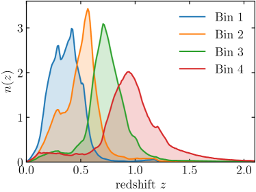
Figure 1: Redshift distributions for the four tomographic bins. See Table 2.

3 Data

The Dark Energy Survey (DES) conducted its six-year survey finalising in January 2019 using a 570-megapixel camera mounted on the 4-meter Blanco Telescope at the Cerro Tololo Inter-American Observatory (CTIO). The photometric survey used five filters and collected information of more than 300 million galaxies in an area of roughly 5000 deg², allowing for the measurement of shapes in addition to positions of galaxies.

The analysis of the first year of data , denoted by DES-Y1, used two independent pipelines (Zuntz et al., 2018) to produce shape catalogues for its shear analysis: metacalibration (Huff & Mandelbaum, 2017; Sheldon & Huff, 2017) and im3shape (Zuntz et al., 2013). Here we will focus on the metacalibration catalogue that was used in the real-space fiducial analysis, with a final contiguous area of 1321 deg² containing 26 million galaxies with a density of 5.5 galaxies arcmin^-2. A Bayesian Photometric Redshift (BPZ) (Benítez, 2000) method was used to divide these source objects into four tomographic redshift bins shown in Table 2 with redshift distributions shown in Figure 1. The priors on the redshift (Hoyle et al., 2018; Davis et al., 2017; Gatti et al., 2018) and shear calibration (Zuntz et al., 2018) parameters are shown in the Table 1.

In order to correct noise, modelling, and selection biases in the shear estimate, one uses the metacalibration method (Huff & Mandelbaum, 2017; Sheldon & Huff, 2017). It introduces a shear response correction (a $2\times 2$ matrix $R_{i}$ for each object $i$) that is obtained by artificially shearing each image in the catalogue and has two components: a response of the shape estimator and a response of the selection of the objects. The DES Y1 metacalibration catalogue does not implement any per-galaxy weight and the shear response corrections are made available in the catalogue release. The shear response is used to obtain the estimated calibrated shear $\hat{\vec{\gamma}}_{i}$ for each object from the measured ellipticities as (Zuntz et al., 2018):

$$\hat{\vec{\gamma}}_{i}=\langle R_{i}\rangle^{-1}\vec{e}_{i},$$ (14)

where we use an averaged response matrix for each tomographic redshift bin and have also subtracted a nonzero mean $\left\langle\vec{e}_{i}\right\rangle$ per tomographic bin prior to the shear estimation. The estimated shear per object is pixelated in maps using the HEALPix pixelisation scheme (Górski et al., 2005) with a resolution $N_{side}=1024$ for each redshift bin and the angular power spectrum is measured using NaMASTER (Alonso et al., 2019) as described in Section 5.

4 Lognormal mock catalogues

We use a set of 1200 lognormal realisations generated with the Full-sky Lognormal Astro-fields Simulation Kit (flask ) (Xavier et al., 2016), specially designed for DES Y1 configuration-space analysis (Krause et al., 2017; Troxel et al., 2018) in order to test our pipeline and validate the fiducial covariance presented in this analysis.

The lognormal flask realisations use as input the angular power spectrum for each pair of redshift bins $(i,j)$. Those were computed using CosmoLike (Krause & Eifler, 2017) from a $\Lambda$CDM cosmological model with parameters quoted as fiducial in Table 1 and redshift distributions for four tomographic redshift bins that were used in the paper describing the DES-Y1 methodology (Krause et al., 2017) and the paper reporting DES-Y1 cosmological results from cosmic shear (Troxel et al., 2018).

On top of the one- and two-point distributions, this suite of realisations were also designed to match the reduced skewness of projected fields predicted by perturbation theory at a fiducial scale of $10\,\mathrm{Mpc}\,h^{-1}$, see Friedrich et al. (2018); Krause et al. (2017) for details. This approach has been shown to yield accurate results for DES-Y1 (Krause et al., 2017) and DES-Y3 (Friedrich et al., 2021) two-point observables. We also note that Friedrich et al. (2021) had shown, also in the context of DES analysis, that the non-connected part of the covariance matrix does not cause significant bias in a cosmological analysis.

The flask shear maps are generated using HEALPix with resolution set by an $N_{\mathrm{side}}$ parameter of 4096. We further sample source galaxy positions and ellipticity dispersion for each tomographic bin by matching the observed number density of galaxies $n_{\rm eff}$ and the shape-noise parameter $\sigma_{\rm e}$. The numbers used for the flask mocks are given in Table 2 and are similar to the values used in Troxel et al. (2018).

5 Methods

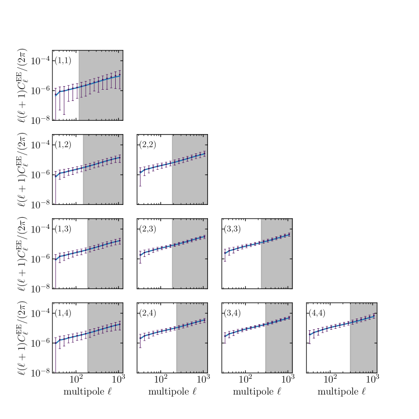
Figure 2: Measured $C_{\ell}^{EE}$ cosmic shear angular power spectra on the 1200 DESY1 flask mocks. Points and error bars show the sample mean and standard deviation for the realizations. The continuous line is obtained from CosmoSIS using the flask cosmology and the vertical shaded regions shows the scale-cuts applied.

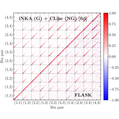
Figure 3: Comparison between our fiducial correlation matrix with the one obtained from the 1200 flask mocks. We show the first 14 bandpower windows for readability and do not apply any scale cuts.

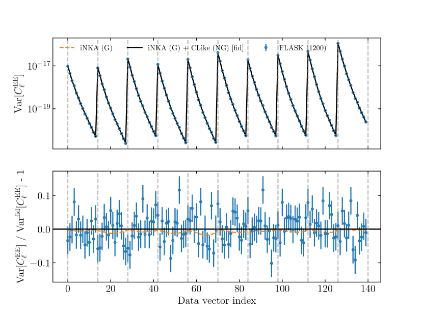
Figure 4: Diagonal elements of the different covariance matrices presented in this work. We show the first 14 bandpower windows for readability and do not apply any scale cuts. The top panel shows the absolute amplitude. Note that iNKA (G) and iNKA (G) + CLike (NG) [fid] lie almost one on top of the other. The bottom panel shows their relative difference. The vertical dashed lines represent the divisions between the different bin pairs considered, ordered as in Figure 3. The DES-Y1 flask mocks sample covariance error bars are computed using the Wishart distribution prediction  (Taylor et al., 2013).

Table 3: Scale-cuts used for the fiducial analysis. The first column shows the tomographic bin pair and the second its scale cuts. We keep the large scale cut, smallest multipole considered, $\ell_{\rm min}$ fixed to $30$ and base our small scale cuts on a conservative one, based on the contribution from baryonic effects. Following (Troxel et al., 2018), we cut bandpowers with a fractional contribution grater than $2\%$ in our fiducial model. We use OWLS AGN simulation (Van Daalen et al., 2011; Schaye et al., 2010) to estimate this contribution.

Bin pair, $(a,b)$	$[\ell_{\rm min}$, $\ell_{\rm max})$
(1, 1)	[30, 150)
(1, 2)	[30, 150)
(1, 3)	[30, 189)
(1, 4)	[30, 189)
(2, 2)	[30, 238)
(2, 3)	[30, 238)
(2, 4)	[30, 189)
(3, 3)	[30, 238)
(3, 4)	[30, 300)
(4, 4)	[30, 300)

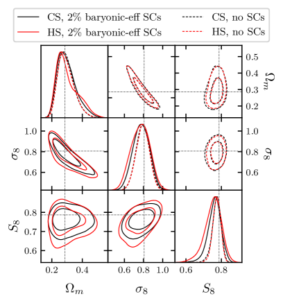
Figure 5: Marginalized posterior distributions for a subset of parameters for a noiseless data vector analyses in both configuration space (CS) and harmonic space (HS), with and without scale cuts (SC) Dashed lines are the input parameters.

In this section, we present the methodology to be used in our analysis. We begin by describing the angular power spectra estimation, followed by a discussion of the scale-cuts chosen to mitigate baryonic effects and end with a discussion of the fiducial covariance matrix used in this work.

5.1 Angular power spectrum measurements

For the angular power spectra estimation, we use the so-called pseudo-$C_{\ell}$ or MASTER method (Peebles, 1973; Brown et al., 2005; Hivon et al., 2002), as implemented in the NaMASTER code  (Alonso et al., 2019).

For the pixelized representation of cosmic shear catalogs, we construct weighted tomographic cosmic shear maps,

$$\vec{\gamma}_{p}=\sum_{i\in p}v_{i}\hat{\vec{\gamma}}_{i}/\sum_{i\in p}v_{i},$$ (15)

where $p$ runs over pixels and $i\in p$ runs over the galaxies in each pixel, $\hat{\vec{\gamma}}_{i}=(\hat{\gamma}_{1},\hat{\gamma}_{2})$ is the calibrated galaxy shear (see eq. (14)) and $v_{i}$ its associated weight. Throughout this work we use a HEALPix fiducial resolution $N_{\mathrm{side}}=1024$, which corresponds to a typical pixel size of the order of $3.4$ arcminutes.

In addition to the cosmic shear signal maps, the pseudo-$C_{\ell}$ method relies on the use of an angular window function, also known as the mask. Such a mask encodes the information of the partial-sky coverage of the observed signal and is used to deconvolve this effect on the estimated bandpowers. In this work, we use the sum of weights scheme presented in Nicola et al. (2021), and construct tomographic mask maps as

$$w_{p}=\sum_{i\in p}v_{i}\ ,$$ (16)

where the $v_{i}$ are the individual galaxy weights assigned by metacalibration. It is important to notice that in this approach there are different masks constructed for each tomographic bin, since the number of galaxies per pixel varies for each bin. In practical terms, these masks are equivalent to the pixelised weighted galaxy-count maps.

An important part of power spectra estimation is the so-called noise bias, always present on the raw signal auto-correlation measurements because of the discrete nature of the signal maps inherited from the galaxy catalogues, giving a Poissonian component. On top of that, for cosmic shear there is also a Gaussian component accounting for any systematic shape noise. For the specific case of the pseudo-$C_{\ell}$ algorithm, the noise bias must be subtracted from the auto-correlations in order to obtain an unbiased estimate of the signal power spectrum. Schematically, the true binned power spectrum estimator can be written as (Alonso et al., 2019):

$$\hat{C}^{ab}_{q}=\sum_{q^{\prime}}({\cal M}^{ab})^{-1}_{qq^{\prime}}\left(\tilde{C}^{ab}_{q^{\prime}}-\delta_{ab}\tilde{N}^{b}_{q^{\prime}}\right),$$ (17)

where $\delta_{ab}$ is the Kronecker delta, ${\cal M}^{ab}_{qq^{\prime}}=\sum_{\ell\in q,\ell^{\prime}\in q^{\prime}}\mathsf{w}_{q}^{\ell}\mathsf{M}^{ab}_{\ell\ell^{\prime}}$ is the binned version of the coupling matrix, $\mathsf{M}^{ab}_{\ell\ell^{\prime}}$, that can be calculated analytically and depends on the mask maps for the tomographic bins $a$ and $b$, $\tilde{C}^{ab}_{q}=\sum_{\ell\in q}\mathsf{w}_{q}^{\ell}\tilde{C}^{ab}_{\ell}$ is the binned version of the pseudo-$C_{\ell}$, $\tilde{C}^{ab}_{\ell}$. Here $q,q^{\prime}$ represent multipole bins or bandpowers and $\mathsf{w}_{q}^{\ell}$ are multipole weights defined for $\ell\in q$ and normalized to $\sum_{\ell\in q}\mathsf{w}_{q}^{\ell}=1$ , see (Alonso et al., 2019) for more details. Finally, $\tilde{N}_{q}=\sum_{\ell\in q}\mathsf{w}_{q}^{\ell}\tilde{N}_{\ell}$ are the binned version of the noise bias pseudo-spectra, $\tilde{N}_{\ell}$, given (in the sum of weights scheme) by (Nicola et al., 2021):

$$\tilde{N}_{\ell}=A_{\rm pix}\left\langle\sum_{i\in p}v_{i}^{2}\sigma_{\gamma,i}^{2}\right\rangle_{\rm pix},$$ (18)

where the average $\left\langle\cdot\right\rangle_{\rm pix}$ is over all the pixels, $A_{\rm pix}$ is the area of the pixels on the chosen HEALPix resolution and

$$\sigma_{\gamma,i}^{2}=\frac{1}{2}\left(\gamma_{1,i}^{2}+\gamma_{2,i}^{2}\right)$$ (19)

is the estimated shear variance of each galaxy. Notice that the noise-bias pseudo-power spectrum $\tilde{N_{\ell}}$ is independent of the $\ell$ multipole. The true noise-bias power spectrum $N_{\ell}$ is obtained using the NaMASTER method, deconvolving the mask and performing the same $\ell$ binning as the signal. This noise bias contribution, subtracted from the measurements, must be included in the covariance matrix, as we will discuss below.

Finally, it is well known that the pixelization process of the shear field can introduce biases in its estimated pseudo-spectra. We correct for the effect of pixelization by dividing the pseudo-spectra by the squared HEALPix pixel window function $F_{\ell}$, i.e, $\tilde{C}^{ab}_{\ell}\to\tilde{C}^{ab}_{\ell}/F_{\ell}^{2}$.

5.2 Binning and scale-cuts

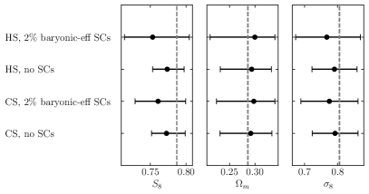
Figure 6: Marginalized constraints for the analyses from a noiseless data vector in harmonic space (HS) and configuration space (CS). We show results without scale cuts (“no SCs" in the figure) and with scale cuts motivated by baryonic effects (“$2\%$ baryonic-eff SCs" in the figure).

For all the angular power spectra measured here, we consider angular multipoles $\ell\in$ [30, 3000) divided into $20$ logarithmic-spaced bandpowers with edges similar to the binning scheme used in Andrade-Oliveira et al. (2021), where analysis of DES-Y1 galaxy clustering in harmonic space is performed.

A comparison between the measured cosmic shear angular power spectra on the mocks and the input theory prediction used for its generation is shown in Figure 2. We find very good agreement, validating the measurement pipeline (namely, the noise-subtraction method and the computation of the coupling matrix).

Scale cuts are a key factor for cosmic shear analyses (see, e.g. Doux et al. (2021b)). For the small scales, we follow the DES-Y1 configuration-space analysis and cut-out scales where baryonic effects introduce a significant bias in the angular power spectra (Troxel et al., 2018). To estimate the impact of baryon physics, the OWLS (OverWhelmingly Large Simulations project) suite of hydrodynamic simulations (Van Daalen et al., 2011; Schaye et al., 2010) is used for re-scaling the computed non-linear power spectrum in our fiducial model prediction by a factor

$$P_{\textrm{NL}}(k)\rightarrow\frac{P_{\textrm{DM}+\textrm{Baryon}}(k)}{P_{\textrm{DM}}(k)}\times P_{\textrm{NL}}(k),$$ (20)

where ‘DM’ refers to the power spectrum from the OWLS dark-matter-only simulation, while ‘DM+Baryon’ refers to the power spectrum from the OWLS AGN simulation (Van Daalen et al., 2011; Schaye et al., 2010). It is important to note that the particular use of the OWLS simulations, among others for DES-Y1 analysis, is a conservative choice, as they offer some of the most significant deviations from the DM cases in the power spectrum Troxel et al. (2018). We then compare the predictions for the cosmic-shear angular power spectra with and without the re-scaling for $P_{NL}(k)$ and impose, for our fiducial analysis, the same $2\%$ threshold imposed by the configuration space analysis (Troxel et al., 2018). Hence we remove from our data vector all bandpowers with a fractional contribution from baryonic effects greater than $2\%$ in our fiducial model for each pair of redshift bins.

We adopt a fiducial value for the lower multipole value $\ell\geq 30$ and test a different value as a robustness test. Our fiducial scale-cuts are summarized in table 3. Our final data vector ends up having a total of 85 entries. We note that an improvement should be expected by including baryonic effects in the modelling and relaxing the proposed scale cuts. As already shown in configuration space (Huang et al., 2021; Moreira et al., 2021) such improvement can be of $\sim 20\%$ on the recovered constraints.

5.3 Covariance matrix

The covariance matrix has Gaussian, non-Gaussian and noise contributions and we use two different methods to compute them. For the Gaussian contribution, we rely on the so-called improved narrow-kernel approximation (iNKA) approach within the pseudo-$C_{\ell}$ framework that takes into account the geometry of the finite survey area described by the mask maps (García-García et al., 2019; Nicola et al., 2021). We also use the full model for the noise terms in the pseudo-spectra Gaussian covariance as given by Nicola et al. (2021) (their equation (2.29)). The non-Gaussian contribution consists of the so-called super-sample covariance (SSC) and the connected part of the 4-point function. These are obtained using the halo model analytical computations with the CosmoLike code (Krause & Eifler, 2017) in harmonic space.

In order to validate our covariance model, we use measurements on the 1200 DES-Y1 flask lognormal mocks to estimate a sample covariance matrix for the angular power spectrum. In Figure 3 we show a comparison between our fiducial covariance matrix (computed at the flask cosmology) and the flask covariance. One can see a good agreement, with the flask covariance being noisier in the non-diagonal elements, as expected.

A more quantitative comparison is presented in Figure 4, where we plot the diagonal elements of the two covariance matrices with error bars obtained from a Wishart distribution. This figure shows that the contribution from the non-Gaussian part to the diagonal of the covariance matrix is negligible in our case.

6 Likelihood analysis

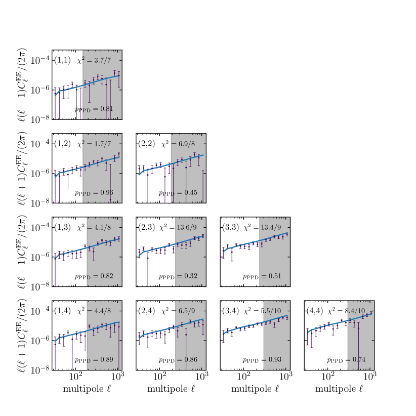
Figure 7: The cosmic shear angular power spectra for the metacalibration catalog. Error-bars are the diagonal elements of the fiducial covariance matrix. The continuous line shows the recovered best-fit model. The vertical shaded region shows the scale-cuts applied. After considering the scale-cuts, the recovered $\chi^{2}$ obtained is 65.5 for 69 degrees of freedom.

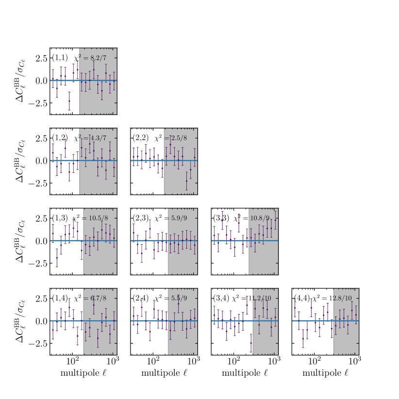
Figure 8: The cosmic-shear $B$-modes angular power spectra for the metacalibration catalog. Error bars are the diagonal elements of the fiducial covariance matrix. The reference is the null model after bandpower binning. The vertical shaded region shows the scale-cuts applied. The goodness of fit for each spectrum is shown on each panel. Combining all the spectra into a single data vector yields a $\chi^{2}=78.3$.

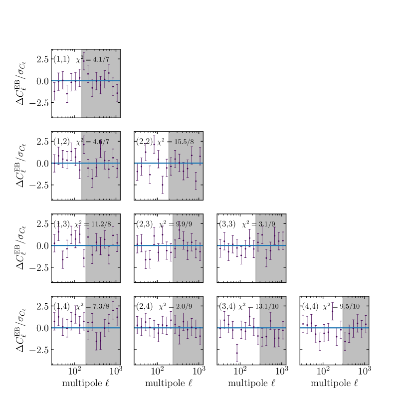
Figure 9: Same as Figure 8 but for the $EB$-modes angular power spectra measured on the metacalibration catalog. Combining all the spectra into a single data vector yields a $\chi^{2}=80.3$.

We have developed a pipeline for Bayesian parameter inference, constructed by adapting the existing DES-Y1 CosmoSIS pipeline developed for a configuration-space analysis (Krause & Eifler, 2017) to perform an analysis in harmonic space. We also use this existing pipeline for all our results quoting configuration space. We use the nested sampling technique for the sampling of Markov Chain Monte Carlo (MCMC) chains. In particular, we use the publicly available Multinest code (Feroz et al., 2009; Feroz et al., 2019). We used a Gaussian likelihood, $L$, defined as

$$-2\log L(\Theta)=\chi^{2}=\sum_{ij}(\hat{D}_{i}-D_{i}(\Theta))^{T}\mathrm{C}^{-1}_{ij}(\hat{D}_{j}-D_{j}(\Theta)),$$ (21)

where $\hat{D}_{i}$ are the entries of the data vector, constructed by stacking the measured power spectra bandpowers $C^{EE(ab)}(\ell)$ for the different combinations of tomographic bins pairs, $(a,b)$, accounting for scale-cuts, see Sections 5.1 and 5.2 and Table 3 and $D_{i}(\Theta)$ are their theoretical predictions computed according to the modelling presented in Section 2. Finally, $\Theta$ represents the set of parameters, cosmological and nuisance, used in the analysis, see Table 1, and $\mathrm{C}$ is the covariance matrix, see Section 5.3.

6.1 Validation with a noiseless data vector

The first step in the analysis is to validate our pipeline using a noiseless analytically computed data vector generated with the flask cosmology. We used our pipeline for the likelihood analyses both in configuration and harmonic space, with and without scale cuts motivated to mitigate baryonic effects and the same binning as described in Section 5.2. This data vector does not contain baryonic effects since the scale cuts were chosen in such a way that they become unimportant, see Section 5.2. Therefore we do not expect baryonic effects to be relevant in our test with the adopted scale cuts, which is why we employed a noiseless data vector. Our aim in this subsection is to test the consistency of the pipeline. For the configuration space run, we follow the DES-Y1 setup (Troxel et al., 2018) again. Figure 5 shows the 2D posterior probability distributions and constraints for a subset of the inferred parameters, namely $S_{8}$, $\Omega_{m}$ and $\sigma_{8}$. Figure 6 provides the 1D marginalized values of the parameters $S_{8}$, $\Omega_{m}$, $\sigma_{8}$, $h_{0}$, $\Omega_{b}$ and $n_{s}$. We conclude that the likelihood pipeline is working as expected in this case, with consistent values for the recovered parameters and error bars.

6.2 Cosmic shear likelihood analysis in DES-Y1

Table 4: The marginalised constraints for the fiducial analysis on configuration and harmonic space. We quote the mean value of the marginalised posterior distribution and the 68% confidence level (CL) around it, as well as the associated $\chi^{2}$. After applying scale-cuts, the data vectors have 227 and 85 elements for the configuration and harmonic space case, respectively. We have 16 model parameters for both cases, yielding 211 and 69 d.o.f. for the CS and HS cases, respectively. These constraints are also presented as error bars in Figure 12.

Case	$\chi^{2}/\mathrm{d.o.f.}$	$\Omega_{m}$	$S_{8}$
HS, Updated cov	65.5/69	$\mathbf{0.304_{-0.042}^{+0.067}}$	$\mathbf{0.766\pm 0.033}$
HS, Fiducial cov	62.8/69	$0.302^{+0.042}_{-0.073}$	$0.765_{-0.036}^{+0.032}$
CS	230.0/211	$0.295^{+0.040}_{-0.059}$	$0.778_{-0.029}^{+0.024}$
HS, Gaussian cov	65.6 / 69	$0.305_{-0.038}^{+0.077}$	$0.767\pm 0.034$
HS, FLASK cov	53 / 69	$0.300_{-0.035}^{+0.066}$	$0.765^{+0.036}_{-0.033}$
HS, $\ell_{\mathrm{min}}=38$	60.5 / 59	$0.287^{+0.035}_{-0.065}$	$0.764_{-0.038}^{+0.033}$
HS, Fixed $\Omega_{\nu}$	65.34 / 70	$0.298_{-0.038}^{+0.066}$	$0.764\pm 0.034$
HS, No IA	66.7 / 71	$0.305_{-0.038}^{+0.077}$	$0.767\pm 0.034$

We now proceed to the likelihood analysis of the DES-Y1 data. The estimated power spectra for DES-Y1 data are shown in fig. 7, along with the recovered best-fit model for our fiducial $\Lambda$CDM results. We begin with a couple of null test validations on the data. First, in the Born approximation, cosmological shear should not produce B-modes. However, in practice, they can be generated by the masking procedure. In Zuntz et al. (2018) it was already shown that the metacalibration catalogue does not contain significant contamination by $B$-modes. Here we extend this tests and verify that the procedure of recovering the true $C_{\ell}^{EE}$ does not introduce significant contributions to $C_{\ell}^{BB}$ in Figure 8 and also $C_{\ell}^{EB}$ in Figure 9. The figure presents the residuals of the measurements with respect to a null model, $\Delta C_{\ell}^{BB/EB}$ normalised by the standard deviation extracted from the fiducial covariance matrix. The measured $C_{\ell}^{BB}$ and $C_{\ell}^{EB}$ are consistent with a null angular power spectrum after the binning procedure with a reasonable $\chi^{2}$ per degree of freedom. We recall here that, to properly account for the binning of the null spectra model in the Pseudo-$C_{\ell}$ estimation context, we follow Alonso et al. (2019) and apply the bandpower window function, as in Equation (13).

Secondly, it is well known that the point spread function (PSF) distorts the images of the galaxies and if not modelled properly, it can lead to significant systematic errors. In order to check its impact on our measurements, we use PSF maps estimated for the DES-Y1 metacalibration catalogue (Zuntz et al., 2018) to estimate its correlation with the $E/B$-mode of the shear signal, $\gamma^{E/B}$. The result is presented in Figure 10, where each column presents the 4 different combinations of the PSF $E/B$ maps and shear $E/B$ maps for a tomographic bin $a\in\{0,1,2,3\}$. As for the previous null test, we summarize the results presenting the residuals with respect to a null signal model normalized by the standard deviation from the fiducial covariance. Our results suggest consistency of these cross-correlations with a null signal. Therefore, we do not apply any further systematic correction on the measured shear spectra.

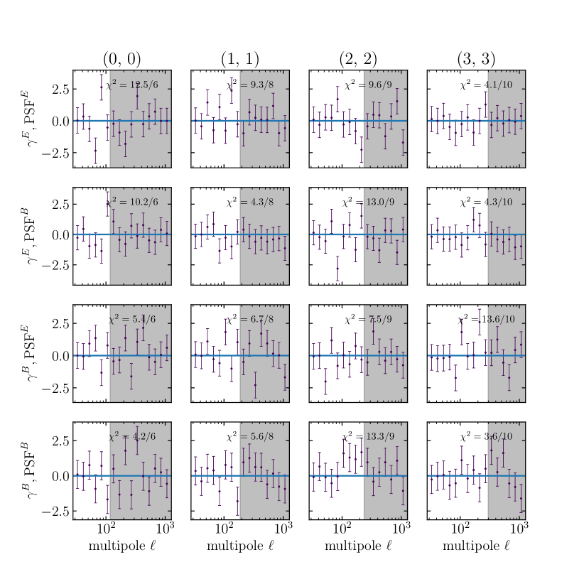
Figure 10: The cosmic-shear correlations between signal and PSF for the metacalibration catalogue. Error bars are the diagonal elements of the fiducial covariance matrix. The reference is the null model after bandpower binning. The vertical shaded region shows the scale-cuts applied. The goodness of fit for each spectrum is shown on each panel.

We then focus on the extraction of cosmological information from the measured $C_{\ell}^{EE}$ power spectra. We vary the six cosmological parameters and the ten nuisance parameters with fiducial values and priors shown in Table 1 . Neutrino masses were varied using three degenerate neutrinos, following Troxel et al. (2018). The nuisance parameters that enter the theoretical modelling of the systematic effects are marginalised to extract cosmological information. We also run the DES-Y1 shear analysis in configuration space to compare the cosmological constraining power of both analyses.

Finally, we re-run the whole harmonic space analysis with an updated covariance matrix, with the Gaussian part computed at the cosmological parameters obtained from the best fit. Our main results are shown in Figures 11, 12 and Table 4 for the 2-D and 1-D marginalized posterior probability distribution on the main cosmological parameters $\Omega_{m}$, $S_{8}$ and $\sigma_{8}$ from a likelihood analysis in both configuration and harmonic space.

We find very good agreement between the two different analyses. The errors are comparable and cosmological parameters are in agreement within less than one standard deviation for both parameter, more precisely, less than $\sim 0.2\,\sigma$ for $\Omega_{m}$ and less than $\sim 0.4\,\sigma$ for $S_{8}$. The $\chi^{2}$ per degree of freedom are consistent and demonstrate a good quality-of-fit for both analyses. The quality-of-fit for each pair of bins are also shown in Figure 7. We also present an additional test on the posterior predictive distribution (PPD), following the methodology presented in Doux et al. (2021a). Namely, the PPD goodness-of-fit test, the probability-to-exceed quantified by the $p$-value, $p_{\rm PPD}$, is also displayed for each pair of bins considered.

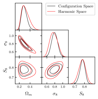
Figure 11: Marginalized posterior distributions for a subset of constrained parameters. We show the results for configuration- and harmonic-space, see Table 4.

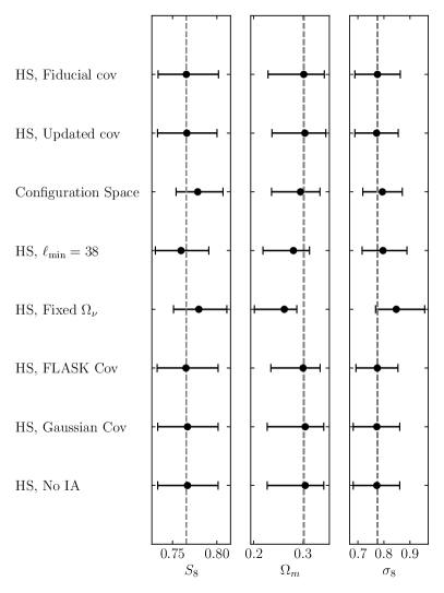
Figure 12: The summary of the one dimensional marginalised constraints on $S_{8}$, $\Omega_{m}$ and $\sigma_{8}$. The 68% CL are shown as error bars around the mean value for the recovered posterior PDF presented as the central point. A battery of robustness tests presented as variations to the fiducial analysis setup are presented. We further present a set of robustness tests representing variations to the fiducial analysis setup are presented. The associated numerical values are presented in Table 4.

On top of well consistent constraints, we found variations of $<1\%$ in the $\chi^{2}$ when consider a pure Gaussian covariance matrix, suggesting a negligible impact for the non-Gaussian corrections in our analysis. This is consistent with results in configuration space (Troxel et al., 2018) and the analysis in harmonic space presented by Nicola et al. (2021). It is important to note that the latter reports variations of $\Delta\chi^{2}\sim 1\%$ but $<10\%$. The lower differences founded here can be understood as a result of our treatment of baryonic effects and the resulting scale cuts.

7 Robustness tests

In this section, we perform a number of robustness tests of our analysis in harmonic space.

• Impact of the covariance cosmology. Our analysis was performed with a theoretical covariance matrix computed at the flask cosmology. In this subsection, we update the covariance matrix to the best-fit cosmological parameters of our analysis in harmonic space and re-run our likelihood pipeline. The results are shown in Figure 12, and there are no significant changes with respect to the original covariance matrix.

  In addition, we also studied the changes in the estimated cosmological parameters arising from using the estimated sample covariance from the suite of lognormal flask realisations. When using this sample covariance, our approach is to use a Gaussian likelihood correcting only the covariance by the Hartlap-Anderson factor (Hartlap et al., 2007). We tested the effect of changing the likelihood to a $t$-student function as motivated by Sellentin & Heavens (2016) founding no appreciable differences. As can be seen in Table 4 again no significant changes are found.

• Scale cuts. Data from large scales are affected by the geometry effects of the mask. These effects are in principle dealt with using the filtering prescription of Alonso et al. (2019) that we adopt here. In this subsection, we test the large scale cuts used in the fiducial choice by leaving out the first $\ell$ bin, using $\ell_{\mathrm{min}}=38$ instead of $\ell_{\mathrm{min}}=30$. As seen in Table 4 again no significant changes are found.

8 Conclusions

We have presented a cosmological analysis using the cosmic shear angular power spectrum obtained from measurements of the DES-Y1 metacalibration shear catalogue. We closely follow the configuration space shear 2-point analysis of Troxel et al. (2018), including the theoretical modelling of redshift uncertainties, shear calibration and intrinsic alignments.

We validated our pipeline using a suite of 1200 lognormal flask mocks. The analysis choices and scale cuts were imposed following a similar prescription for baryon contamination as the configuration space analysis. Our analytical covariance matrix was obtained from combining a Gaussian contribution that incorporates the survey geometry in the so-called improved Narrow-Kernel Approximation (iNKA) approximation with a non-Gaussian contribution from CosmoLike and validated using shear measurements of the 1200 flask mocks. The shape noise contributions to the power spectra and the covariance matrices were estimated analytically following Nicola et al. (2021) using the so-called sum of weights mask scheme, see Section 5.1. We used our pipeline to measure the angular power spectrum $C_{\ell}^{EE}$ in the DES-Y1 metacalibration catalogue and show that it does not introduce significant contributions to $C_{\ell}^{BB}$ and $C_{\ell}^{EB}$.

Finally, we performed a likelihood analysis using the CosmoSIS framework in both configuration space, reproducing the DES-Y1 results, and in harmonic space with a fiducial analysis and also study the impact of variations, such as a covariance matrix computed in a different cosmology, a scale cut on large scales, and a different treatment of neutrino masses. Although the analysis in configuration and harmonic space are independent, we find results for the cosmological parameters $S_{8}$ and $\Omega_{m}$ that are very consistent. Differences were found to be less than $\sim 0.2\,\sigma$ for $\Omega_{m}$ and less than $\sim 0.4\,\sigma$ for $S_{8}$. These results are encouraging and provide a stepping stone to the shear analysis in harmonic space using the third year of DES data (Y3). The DES-Y3 shear analysis in harmonic space will use a similar pipeline but with some improved modelling, mostly following the methodology laid out for the real-space case (Krause et al., 2021) and the real-space shear results (Secco et al., 2022; Amon et al., 2022): an inverse-variance weights determined in the Y3 metacalibration catalogue (Gatti et al., 2021), a tidal alignment and tidal torquing (TATT) model (Blazek et al., 2019) for intrinsic alignment, a determination of scale cuts using a $\chi^{2}$ criterion between noiseless data vectors with and without baryon effect contamination, the usage of a blinding strategy and more robustness tests. The results will be addressed in a forthcoming publication.

Data Availability Statement

The DES Y1 catalog is available in the Dark Energy Survey Data Management (DESDM) system at the National Center for Supercomputing Applications (NCSA) at the University of Illinois. It can be accessed at https://des.ncsa.illinois.edu/releases/y1a1/key-catalogs. The pipeline used for the measurement is publicly available at https://github.com/hocamachoc/3x2hs_measurements. Synthetic data produced by the analysis presented here can be shared on request to the corresponding author.

Author Affiliations

¹ Instituto de Física Teórica, Universidade Estadual Paulista, São Paulo, Brazil
² Laboratório Interinstitucional de e-Astronomia - LIneA, Rua Gal. José Cristino 77, Rio de Janeiro, RJ - 20921-400, Brazil
³ ICTP South American Institute for Fundamental Research
Instituto de Física Teórica, Universidade Estadual Paulista, São Paulo, Brazil
⁴ Departamento de Física Matemática, Instituto de Física, Universidade de São Paulo, CP 66318, São Paulo, SP, 05314-970, Brazil
⁵ Department of Physics and Astronomy, University of Pennsylvania, Philadelphia, PA 19104, USA
⁶ Department of Astronomy, University of California, Berkeley, 501 Campbell Hall, Berkeley, CA 94720, USA
⁷ Department of Astronomy/Steward Observatory, University of Arizona, 933 North Cherry Avenue, Tucson, AZ 85721-0065, USA
⁸ Jet Propulsion Laboratory, California Institute of Technology, 4800 Oak Grove Dr., Pasadena, CA 91109, USA
⁹ Kavli Institute for Cosmology, University of Cambridge, Madingley Road, Cambridge CB3 0HA, UK
¹⁰ Department of Physics, Northeastern University, Boston, MA 02115, USA
¹¹ Laboratory of Astrophysics, École Polytechnique Fédérale de Lausanne (EPFL), Observatoire de Sauverny, 1290 Versoix, Switzerland
¹² Jodrell Bank Center for Astrophysics, School of Physics and Astronomy, University of Manchester, Oxford Road, Manchester, M13 9PL, UK
¹³ California Institute of Technology, 1200 East California Blvd, MC 249-17, Pasadena, CA 91125, USA
¹⁴ Kavli Institute for Particle Astrophysics & Cosmology, P. O. Box 2450, Stanford University, Stanford, CA 94305, USA
¹⁵ Lawrence Berkeley National Laboratory, 1 Cyclotron Road, Berkeley, CA 94720, USA
¹⁶ Institut d’Estudis Espacials de Catalunya (IEEC), 08034 Barcelona, Spain
¹⁷ Institute of Space Sciences (ICE, CSIC), Campus UAB, Carrer de Can Magrans, s/n, 08193 Barcelona, Spain
¹⁸ Faculty of Physics, Ludwig-Maximilians-Universität, Scheinerstr. 1, 81679 Munich, Germany
¹⁹ Department of Astronomy, University of Geneva, ch. d’Écogia 16, CH-1290 Versoix, Switzerland
²⁰ Department of Applied Mathematics and Theoretical Physics, University of Cambridge, Cambridge CB3 0WA, UK
²¹ Department of Astronomy and Astrophysics, University of Chicago, Chicago, IL 60637, USA
²² Kavli Institute for Cosmological Physics, University of Chicago, Chicago, IL 60637, USA
²³ Department of Physics, Carnegie Mellon University, Pittsburgh, Pennsylvania 15312, USA
²⁴ Brookhaven National Laboratory, Bldg 510, Upton, NY 11973, USA
²⁵ Department of Physics, Duke University Durham, NC 27708, USA
²⁶ Institut de Física d’Altes Energies (IFAE), The Barcelona Institute of Science and Technology, Campus UAB, 08193 Bellaterra (Barcelona) Spain
²⁷ Institute for Astronomy, University of Edinburgh, Edinburgh EH9 3HJ, UK
²⁸ Cerro Tololo Inter-American Observatory, NSF’s National Optical-Infrared Astronomy Research Laboratory, Casilla 603, La Serena, Chile
²⁹ Fermi National Accelerator Laboratory, P. O. Box 500, Batavia, IL 60510, USA
³⁰ Institute of Cosmology and Gravitation, University of Portsmouth, Portsmouth, PO1 3FX, UK
³¹ CNRS, UMR 7095, Institut d’Astrophysique de Paris, F-75014, Paris, France
³² Sorbonne Universités, UPMC Univ Paris 06, UMR 7095, Institut d’Astrophysique de Paris, F-75014, Paris, France
³³ Department of Physics & Astronomy, University College London, Gower Street, London, WC1E 6BT, UK
³⁴ SLAC National Accelerator Laboratory, Menlo Park, CA 94025, USA
³⁵ Center for Astrophysical Surveys, National Center for Supercomputing Applications, 1205 West Clark St., Urbana, IL 61801, USA
³⁶ Department of Astronomy, University of Illinois at Urbana-Champaign, 1002 W. Green Street, Urbana, IL 61801, USA
³⁷ Physics Department, William Jewell College, Liberty, MO, 64068, USA
³⁸ Astronomy Unit, Department of Physics, University of Trieste, via Tiepolo 11, I-34131 Trieste, Italy
³⁹ INAF-Osservatorio Astronomico di Trieste, via G. B. Tiepolo 11, I-34143 Trieste, Italy
⁴⁰ Institute for Fundamental Physics of the Universe, Via Beirut 2, 34014 Trieste, Italy
⁴¹ Observatório Nacional, Rua Gal. José Cristino 77, Rio de Janeiro, RJ - 20921-400, Brazil
⁴² Department of Physics, University of Michigan, Ann Arbor, MI 48109, USA
⁴³ Hamburger Sternwarte, Universität Hamburg, Gojenbergsweg 112, 21029 Hamburg, Germany
⁴⁴ Centro de Investigaciones Energéticas, Medioambientales y Tecnológicas (CIEMAT), Madrid, Spain
⁴⁵ Department of Physics, IIT Hyderabad, Kandi, Telangana 502285, India
⁴⁶ Santa Cruz Institute for Particle Physics, Santa Cruz, CA 95064, USA
⁴⁷ Department of Astronomy, University of Michigan, Ann Arbor, MI 48109, USA
⁴⁸ Institute of Theoretical Astrophysics, University of Oslo. P.O. Box 1029 Blindern, NO-0315 Oslo, Norway
⁴⁹ Instituto de Fisica Teorica UAM/CSIC, Universidad Autonoma de Madrid, 28049 Madrid, Spain
⁵⁰ School of Mathematics and Physics, University of Queensland, Brisbane, QLD 4072, Australia
⁵¹ Center for Cosmology and Astro-Particle Physics, The Ohio State University, Columbus, OH 43210, USA
⁵² Department of Physics, The Ohio State University, Columbus, OH 43210, USA
⁵³ Center for Astrophysics $|$ Harvard & Smithsonian, 60 Garden Street, Cambridge, MA 02138, USA
⁵⁴ Australian Astronomical Optics, Macquarie University, North Ryde, NSW 2113, Australia
⁵⁵ Lowell Observatory, 1400 Mars Hill Rd, Flagstaff, AZ 86001, USA
⁵⁶ George P. and Cynthia Woods Mitchell Institute for Fundamental Physics and Astronomy, and Department of Physics and Astronomy, Texas A&M University, College Station, TX 77843, USA
⁵⁷ Department of Astrophysical Sciences, Princeton University, Peyton Hall, Princeton, NJ 08544, USA
⁵⁸ Institució Catalana de Recerca i Estudis Avançats, E-08010 Barcelona, Spain
⁵⁹ Physics Department, 2320 Chamberlin Hall, University of Wisconsin-Madison, 1150 University Avenue Madison, WI 53706-1390
⁶⁰ Institute of Astronomy, University of Cambridge, Madingley Road, Cambridge CB3 0HA, UK
⁶¹ School of Physics and Astronomy, University of Southampton, Southampton, SO17 1BJ, UK
⁶² Computer Science and Mathematics Division, Oak Ridge National Laboratory, Oak Ridge, TN 37831
⁶³ Department of Physics, Stanford University, 382 Via Pueblo Mall, Stanford, CA 94305, USA
⁶⁴ Max Planck Institute for Extraterrestrial Physics, Giessenbachstrasse, 85748 Garching, Germany
⁶⁵ Universitäts-Sternwarte, Fakultät für Physik, Ludwig-Maximilians Universität München, Scheinerstr. 1, 81679 München, Germany
⁶⁶ Department of Physics and Astronomy, Pevensey Building, University of Sussex, Brighton, BN1 9QH, UK

Appendix A Residual systematics in the cosmic shear signal

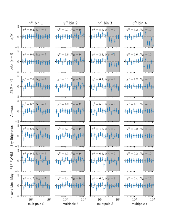
Figure 13: Testing for residual systematics in the tomographic cosmic shear signal in harmonic space Each panel shows measured cross-correlation of the different tomographic bins considered in this work (columns) and a subsample of survey properties most likely to be sourcing residual shear systematics (rows). The fiducial analysis used the same bandpower binning and scale cuts (shaded regions). The significance of the null-test, $\chi^{2}$, and the number of elements in the data vector are shown in each panel.

The DES Y1 metacalibration catalogue has been carefully designed for testing for systematics under a battery of null tests (Zuntz et al., 2018), resulting in the advice of accounting for possible photo-z and shear estimation systematic biases as done in the present work. However, potential residual systematics biases that have not been identified can persist. Following the DES SV (Becker et al., 2016) and DES Y1 (Troxel et al., 2018) cosmic shear analyses in configuration space, we test those by considering a subsample of survey properties that are most likely to be sourcing residual shear systematics. On top of the PSF ellipticity presented in 7, we consider signal-to-noise ($S/N$), $r-i$ color, dust extinction ($E(B-V)$), sky brightness, PSF size (PSF FWHM), airmass, and $r$-band limiting magnitude. The first four are intrinsic properties of each galaxy image measured by the DES Y1 shape and PSF measurement pipelines (Zuntz et al., 2018). The last five are the mean value of each property across exposures at a given position in the sky. We generated HEALPix maps for those properties with the same HEALPix resolution of our measurements, NSIDE of 1024. As in (Troxel et al., 2018), we do not consider several properties tested in the DES SV analysis because of their high degeneracy with the considered ones. Also, as catalogue preparation for DES Y1 data found no need to make an explicit surface brightness cut in the shape catalogues (Zuntz et al., 2018), we do not consider that property.

Our methodology is, however, different from the one from configuration space analyses. We consider the cross-correlation between the observed shear signal and the survey properties and test for a null hypothesis quantified in the $\chi^{2}$ using the fiducial covariance and scale-cuts of the analysis.

We present our result in the Figure 13, where the estimated cross-correlations normalised by the error bars are presented. The figure also quotes the significance, $\chi^{2}$, and the number of points in the considered data vector, $N_{D}$. There is no strong evidence of cross correlation between survey properties and the shear signal in any of the tomographic bins.

For the intrinsic properties of each galaxy image, $S/N$ and color, there does seem to be higher significance for cross-correlation in the highest redshift bin for the smallest scales, cut out by the scale-cuts in our analysis. For the rest of the properties, our first bandpower, $[30,37)$, exhibits the most considerable significance of cross-correlation, not statistically significant when combined with the rest of the data vector for any of the cases.

Appendix B Full marginalized 2D and 1D posteriors

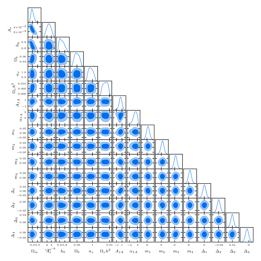
Figure 14: The full marginalized 2D and 1D posterior PDF for all 16 parameters in our fiducial $\Lambda$CDM model. The 2D contours show the 68% and 95% confidence intervals.

We show all the marginalised 2D and 1D posteriors for the full parameter space of our fiducial $\Lambda$CDM analysis in Figure 14. No significant constraint beyond the prior was found for all the nuisance parameters, $m_{i},\Delta z_{i}$, nor for $h_{0},\Omega_{b},n_{s},\Omega_{\nu}h^{2}$.

References

- Abbott et al. (2022) Abbott T. M. C., et al., 2022, Phys. Rev. D, 105, 043512
- Alonso et al. (2019) Alonso D., Sanchez J., Slosar A., LSST Dark Energy Science Collaboration 2019, MNRAS, 484, 4127
- Amon et al. (2022) Amon A., et al., 2022, Phys. Rev. D, 105, 023514
- Andrade-Oliveira et al. (2021) Andrade-Oliveira F., et al., 2021, MNRAS, 505, 5714
- Asgari et al. (2021) Asgari M., et al., 2021, A&A, 645, A104
- Bartelmann & Schneider (2001) Bartelmann M., Schneider P., 2001, Phys. Rep., 340, 291
- Becker et al. (2016) Becker M. R., et al., 2016, Phys. Rev. D, 94, 022002
- Benítez (2000) Benítez N., 2000, ApJ, 536, 571
- Blazek et al. (2019) Blazek J. A., MacCrann N., Troxel M. A., Fang X., 2019, Phys. Rev. D, 100, 103506
- Bridle & King (2007) Bridle S., King L., 2007, New Journal of Physics, 9, 444
- Brown et al. (2005) Brown M. L., Castro P. G., Taylor A. N., 2005, MNRAS, 360, 1262
- Chang et al. (2018) Chang C., et al., 2018, MNRAS, 475, 3165
- Chang et al. (2019) Chang C., et al., 2019, MNRAS, 482, 3696
- Van Daalen et al. (2011) Van Daalen M. P., Schaye J., Booth C. M., Dalla Vecchia C., 2011, MNRAS, 415, 3649
- Davis et al. (2017) Davis C., et al., 2017, arXiv e-prints, p. arXiv:1710.02517
- Dodelson (2017) Dodelson S., 2017, Gravitational Lensing. Cambridge University Press
- Doux et al. (2021a) Doux C., et al., 2021a, MNRAS, 503, 2688
- Doux et al. (2021b) Doux C., et al., 2021b, MNRAS, 503, 3796
- Doux et al. (2022) Doux C., et al., 2022, MNRAS, 515, 1942
- Dyson et al. (1920) Dyson F. W., Eddington A. S., Davidson C., 1920, Philosophical Transactions of the Royal Society of London Series A, 220, 291
- Einstein (1916) Einstein A., 1916, Annalen Phys., 49, 769
- Feroz et al. (2009) Feroz F., Hobson M. P., Bridges M., 2009, MNRAS, 398, 1601
- Feroz et al. (2019) Feroz F., Hobson M. P., Cameron E., Pettitt A. N., 2019, The Open Journal of Astrophysics, 2, 10
- Friedrich et al. (2018) Friedrich O., et al., 2018, Phys. Rev. D, 98, 023508
- Friedrich et al. (2021) Friedrich O., et al., 2021, MNRAS, 508, 3125
- García-García et al. (2019) García-García C., Alonso D., Bellini E., 2019, J. Cosmology Astropart. Phys., 2019, 043
- Gatti et al. (2018) Gatti M., et al., 2018, MNRAS, 477, 1664
- Gatti et al. (2021) Gatti M., et al., 2021, MNRAS, 504, 4312
- Górski et al. (2005) Górski K. M., Hivon E., Banday A. J., Wandelt B. D., Hansen F. K., Reinecke M., Bartelmann M., 2005, ApJ, 622, 759
- Hadzhiyska et al. (2021) Hadzhiyska B., García-García C., Alonso D., Nicola A., Slosar A., 2021, J. Cosmology Astropart. Phys., 2021, 020
- Hamana et al. (2020) Hamana T., et al., 2020, PASJ, 72, 16
- Hamana et al. (2022) Hamana T., et al., 2022, PASJ, 74, 488
- Harris et al. (2020) Harris C. R., et al., 2020, Nature, 585, 357
- Hartlap et al. (2007) Hartlap J., Simon P., Schneider P., 2007, A&A, 464, 399
- Heymans et al. (2006) Heymans C., et al., 2006, MNRAS, 368, 1323
- Hikage et al. (2019) Hikage C., et al., 2019, PASJ, 71, 43
- Hildebrandt et al. (2017) Hildebrandt H., et al., 2017, MNRAS, 465, 1454
- Hivon et al. (2002) Hivon E., Górski K. M., Netterfield C. B., Crill B. P., Prunet S., Hansen F., 2002, ApJ, 567, 2
- Howlett et al. (2012) Howlett C., Lewis A., Hall A., Challinor A., 2012, J. Cosmology Astropart. Phys., 2012, 027
- Hoyle et al. (2018) Hoyle B., et al., 2018, MNRAS, 478, 592
- Huang et al. (2021) Huang H.-J., et al., 2021, MNRAS, 502, 6010
- Huff & Mandelbaum (2017) Huff E., Mandelbaum R., 2017, arXiv e-prints, p. arXiv:1702.02600
- Hunter (2007) Hunter J. D., 2007, Computing in Science and Engineering, 9, 90
- Huterer et al. (2006) Huterer D., Takada M., Bernstein G., Jain B., 2006, MNRAS, 366, 101
- Jee et al. (2013) Jee M. J., Tyson J. A., Schneider M. D., Wittman D., Schmidt S., Hilbert S., 2013, ApJ, 765, 74
- Jee et al. (2016) Jee M. J., Tyson J. A., Hilbert S., Schneider M. D., Schmidt S., Wittman D., 2016, ApJ, 824, 77
- Joachimi et al. (2015) Joachimi B., et al., 2015, Space Sci. Rev., 193, 1
- Joachimi et al. (2021) Joachimi B., et al., 2021, A&A, 646, A129
- Joudaki et al. (2017) Joudaki S., et al., 2017, MNRAS, 465, 2033
- Joudaki et al. (2020) Joudaki S., et al., 2020, A&A, 638, L1
- Kaiser (1992) Kaiser N., 1992, ApJ, 388, 272
- Kilbinger (2015) Kilbinger M., 2015, Reports on Progress in Physics, 78, 086901
- Kilbinger et al. (2017) Kilbinger M., et al., 2017, MNRAS, 472, 2126
- Kirk et al. (2012) Kirk D., Rassat A., Host O., Bridle S., 2012, MNRAS, 424, 1647
- Kitching et al. (2017) Kitching T. D., Alsing J., Heavens A. F., Jimenez R., McEwen J. D., Verde L., 2017, MNRAS, 469, 2737
- Krause & Eifler (2017) Krause E., Eifler T., 2017, MNRAS, 470, 2100
- Krause et al. (2017) Krause E., et al., 2017, arXiv e-prints, p. arXiv:1706.09359
- Krause et al. (2021) Krause E., et al., 2021, arXiv e-prints, p. arXiv:2105.13548
- Lemos et al. (2017) Lemos P., Challinor A., Efstathiou G., 2017, J. Cosmology Astropart. Phys., 2017, 014
- Lewis et al. (2000) Lewis A., Challinor A., Lasenby A., 2000, ApJ, 538, 473
- Limber (1953) Limber D. N., 1953, ApJ, 117, 134
- LoVerde & Afshordi (2008) LoVerde M., Afshordi N., 2008, Phys. Rev. D, 78, 123506
- Loureiro et al. (2021) Loureiro A., et al., 2021, arXiv e-prints, p. arXiv:2110.06947
- Mandelbaum (2018) Mandelbaum R., 2018, ARA&A, 56, 393
- Moreira et al. (2021) Moreira M. G., Andrade-Oliveira F., Fang X., Huang H.-J., Krause E., Miranda V., Rosenfeld R., Simonović M., 2021, MNRAS, 507, 5592
- Nicola et al. (2021) Nicola A., García-García C., Alonso D., Dunkley J., Ferreira P. G., Slosar A., Spergel D. N., 2021, J. Cosmology Astropart. Phys., 2021, 067
- Peebles (1973) Peebles P. J. E., 1973, ApJ, 185, 413
- Schaye et al. (2010) Schaye J., et al., 2010, MNRAS, 402, 1536
- Secco et al. (2022) Secco L. F., et al., 2022, Phys. Rev. D, 105, 023515
- Sellentin & Heavens (2016) Sellentin E., Heavens A. F., 2016, MNRAS, 456, L132
- Sheldon & Huff (2017) Sheldon E. S., Huff E. M., 2017, ApJ, 841, 24
- Smith et al. (2003) Smith R. E., et al., 2003, MNRAS, 341, 1311
- Takahashi et al. (2012) Takahashi R., Sato M., Nishimichi T., Taruya A., Oguri M., 2012, ApJ, 761, 152
- Taylor et al. (2013) Taylor A., Joachimi B., Kitching T., 2013, MNRAS, 432, 1928
- Troxel & Ishak (2015) Troxel M. A., Ishak M., 2015, Phys. Rep., 558, 1
- Troxel et al. (2018) Troxel M. A., et al., 2018, Phys. Rev. D, 98, 043528
- Xavier et al. (2016) Xavier H. S., Abdalla F. B., Joachimi B., 2016, MNRAS, 459, 3693
- Zuntz et al. (2013) Zuntz J., Kacprzak T., Voigt L., Hirsch M., Rowe B., Bridle S., 2013, MNRAS, 434, 1604
- Zuntz et al. (2015) Zuntz J., et al., 2015, Astronomy and Computing, 12, 45
- Zuntz et al. (2018) Zuntz J., et al., 2018, MNRAS, 481, 1149