e-mail: ]namitana@usc.edu
e-mail: ]zanardi@usc.edu
BROTOCs and Quantum Information Scrambling at Finite Temperature
Abstract
Out-of-time-ordered correlators (OTOCs) have been extensively studied in recent years as a diagnostic of quantum information scrambling. In this paper, we study quantum information-theoretic aspects of the regularized finite-temperature OTOC. We introduce analytical results for the bipartite regularized OTOC (BROTOC): the regularized OTOC averaged over random unitaries supported over a bipartition. We show that the BROTOC has several interesting properties, for example, it quantifies the purity of the associated thermofield double state and the “operator purity” of the analytically continued time-evolution operator. At infinite-temperature, it reduces to one minus the operator entanglement of the time-evolution operator. In the zero-temperature limit and for nondegenerate Hamiltonians, the BROTOC probes the groundstate entanglement. By computing long-time averages, we show that the equilibration value of the BROTOC is intimately related to eigenstate entanglement. Finally, we numerically study the equilibration value of the BROTOC for various physically relevant Hamiltonian models and comment on its ability to distinguish integrable and chaotic dynamics.
1 Introduction
The thermalization of closed quantum systems has been a long standing puzzle in theoretical physics [Srednicki(1994), Rigol et al.(2008)Rigol, Dunjko, and Olshanii, D’Alessio et al.(2016)D’Alessio, Kafri, Polkovnikov, and Rigol, Borgonovi et al.(2016)Borgonovi, Izrailev, Santos, and Zelevinsky]. Recently, the notion of “information scrambling” as the underlying mechanism for thermalization has gained prominence. The idea is that complex quantum systems quickly disseminate localized information through the (nonlocal) degrees of freedom, making it inaccessible to any local probes to the system. The information is not lost, since the global evolution is still unitary, rather, it is encoded in nonlocal correlations across the system. A quantification of this dynamical phenomena has initated a rich discussion surrounding operator growth [von Keyserlingk et al.(2018)von Keyserlingk, Rakovszky, Pollmann, and Sondhi, Nahum et al.(2018)Nahum, Vijay, and Haah, Rakovszky et al.(2018)Rakovszky, Pollmann, and von Keyserlingk, Khemani et al.(2018a)Khemani, Vishwanath, and Huse, Gopalakrishnan et al.(2018)Gopalakrishnan, Huse, Khemani, and Vasseur, Chan et al.(2018)Chan, De Luca, and Chalker, Parker et al.(2019)Parker, Cao, Avdoshkin, Scaffidi, and Altman], eigenstate thermalization hypothesis (ETH) [Murthy and Srednicki(2019)], quantum chaos [Maldacena et al.(2016)Maldacena, Shenker, and Stanford, Xu et al.(2020)Xu, Scaffidi, and Cao], among others; see also Refs. [Swingle(2018), Xu and Swingle(2022)] for a recent review. One of the central objects in this quantification are the so-called out-of-time-ordered correlators (OTOCs). The OTOC is usually defined as a four point function with unusual time-ordering [Larkin and Ovchinnikov(1969), Kitaev(2015)],
| (1) |
where is the Heisenberg-evolved operator and is the Gibbs state at inverse temperature with . An intimately related quantity to the above OTOC is the following norm of the commutator,
| (2) |
Here we have used the Hilbert-Schmidt norm , which originates from the (Hilbert-Schmidt) inner product . The two quantities are related via the simple formula,
| (3) |
Therefore, the growth of the norm of the commutator is associated to the decay of the OTOCs.
The idea behind using the norm of the commutator to quantify scrambling is the following: let and be two local operators that initially commute (for example, consider local operators on two different sites of a quantum spin-chain). Under Heisenberg time-evolution, the support of grows and after a transient period, it will start noncommuting with the operator and one can utilize the commutator to quantify this growth. Intuitively, if the Hamiltonian of this system is local, then Leib-Robinson type bounds can provide an estimate for the time it takes for the growth of this commutator [Lieb and Robinson(1972), Hastings and Koma(2006), Bravyi et al.(2006)Bravyi, Hastings, and Verstraete].
Understanding quantitatively, the scrambling of quantum information has lead to a plethora of theoretical insights [Maldacena et al.(2016)Maldacena, Shenker, and Stanford, Cotler et al.(2017a)Cotler, Hunter-Jones, Liu, and Yoshida, Hosur et al.(2016)Hosur, Qi, Roberts, and Yoshida, von Keyserlingk et al.(2018)von Keyserlingk, Rakovszky, Pollmann, and Sondhi, Nahum et al.(2018)Nahum, Vijay, and Haah, Rakovszky et al.(2018)Rakovszky, Pollmann, and von Keyserlingk, Khemani et al.(2018a)Khemani, Vishwanath, and Huse, Gopalakrishnan et al.(2018)Gopalakrishnan, Huse, Khemani, and Vasseur, Chan et al.(2018)Chan, De Luca, and Chalker, Parker et al.(2019)Parker, Cao, Avdoshkin, Scaffidi, and Altman, Murthy and Srednicki(2019)]. This was swiftly followed by several state-of-the-art experimental investigations [Mi et al.(2021)Mi, Roushan, Quintana, Mandra, Marshall, Neill, Arute, Arya, Atalaya, Babbush et al., Braumüller et al.(2022)Braumüller, Karamlou, Yanay, Kannan, Kim, Kjaergaard, Melville, Niedzielski, Sung, Vepsäläinen et al., Wei et al.(2018)Wei, Ramanathan, and Cappellaro, Li et al.(2017)Li, Fan, Wang, Ye, Zeng, Zhai, Peng, and Du, Nie et al.(2019)Nie, Zhang, Zhao, Xin, Lu, and Li, Nie et al.(2020)Nie, Wei, Chen, Zhang, Zhao, Qiu, Tian, Ji, Xin, Lu, and Li, Gärttner et al.(2017)Gärttner, Bohnet, Safavi-Naini, Wall, Bollinger, and Rey, Joshi et al.(2020)Joshi, Elben, Vermersch, Brydges, Maier, Zoller, Blatt, and Roos, Meier et al.(2019)Meier, Ang’ong’a, An, and Gadway, Chen et al.(2020)Chen, Hou, Zhou, Qian, Shen, and Xu]. Furthermore, several works have now elucidated quantum information theoretic aspects underlying the OTOC, for example, by connecting it to Loschmidt Echo [Yan et al.(2020)Yan, Cincio, and Zurek], operator entanglement and entropy production [Styliaris et al.(2021)Styliaris, Anand, and Zanardi, Zanardi and Anand(2021)], quantum coherence [Anand et al.(2021)Anand, Styliaris, Kumari, and Zanardi], entropic uncertainty relations [Yunger Halpern et al.(2019)Yunger Halpern, Bartolotta, and Pollack], among others.
In Refs. [Yan et al.(2020)Yan, Cincio, and Zurek, Styliaris et al.(2021)Styliaris, Anand, and Zanardi], the authors defined a “bipartite OTOC,” obtained by averaging the infinite-temperature OTOC uniformly over local random unitaries supported on a bipartition. In Ref. [Styliaris et al.(2021)Styliaris, Anand, and Zanardi], this bipartite OTOC was shown to have the following operational interpretations: (i) it is exactly the operator entanglement [Zanardi(2001), Wang and Zanardi(2002)] of the dynamical unitary , (ii) it connects in a simple way to the entangling power [Zanardi et al.(2000)Zanardi, Zalka, and Faoro] of the dynamical unitary , (iii) it is exactly equal to the average linear entropy production power of the reduced dynamics, among others. Furthermore, several of these connections were generalized to the case of open-system dynamics in Ref. [Zanardi and Anand(2021)], where, in particular, a competition between information scrambling and environmental decoherence was uncovered [Touil and Deffner(2021)].
Unfortunately, as we move away from the infinite-temperature assumption, the connections unveiled in Ref. [Styliaris et al.(2021)Styliaris, Anand, and Zanardi] do not carry over their operational aspects anymore. For example, a straightforward generation to the finite temperature case, say, by using the OTOC as defined in Eq. 1 fails to retain the operator entanglement or entropy production connection. Not all is lost, however, as it is the regularized OTOC [Maldacena et al.(2016)Maldacena, Shenker, and Stanford] that naturally lends itself to these operational connections. Elucidating this connection is the key technical contribution of this work. For ease of readability, the proofs of key Propositions appear in the Appendix.
2 Preliminaries
The OTOC introduced in Eq. 1 will hereafter be referred to as the unregularized OTOC. In contrast, the regularized (or symmetric) OTOC is defined as [Maldacena et al.(2016)Maldacena, Shenker, and Stanford],
| (4) |
Equivalently,
| (5) |
with . We also define the associated disconnected correlator [Maldacena et al.(2016)Maldacena, Shenker, and Stanford],
| (6) |
In Ref. [Maldacena et al.(2016)Maldacena, Shenker, and Stanford], a bound on the growth of the correlator was obtained under certain assumptions as
| (7) |
We also refer the reader to Ref. [Murthy and Srednicki(2019)] the same bound was derived for systems satisfying ETH, along with some extra assumptions. In this work we focus on the quantity arising from this bound and connect it to operational, quantum information-theoretic quantities. Notice that, for a time-independent Hamiltonian, the disconnected correlator is time independent (by using the commutation of and the cyclicity of trace). Therefore, we can define, .
Following Ref. [Styliaris et al.(2021)Styliaris, Anand, and Zanardi], we will consider the following setup: let be a bipartition of the Hilbert space. Define as , the unitary group over . We want to understand the qualitative and quantitative features of the OTOC for a generic choice of local operators and . Therefore, we average over unitary operators supported on the bipartition . We define the bipartite averaged, unregularized OTOC (hereafter, bipartite unregularized OTOC) as [Styliaris et al.(2021)Styliaris, Anand, and Zanardi]
| (8) |
where, , with and denotes Haar-averaging over the standard uniform measure over [Watrous(2018)]. In Ref. [Styliaris et al.(2021)Styliaris, Anand, and Zanardi] it was shown that one can analytically perform the Haar averages to obtain the following expression,
| (9) |
where is the operator that swaps the spaces in . This equation represents the finite temperature version of the unregularized bipartite OTOC. For , this is the operator entanglement of the time evolution operator as will be discussed shortly. However, for , it does not have a clear quantum information-theoretic correspondence.
Ref. [Styliaris et al.(2021)Styliaris, Anand, and Zanardi] studied in extensive detail at . Here, we will contrast the dynamical behavior of the bipartite unregularized OTOC with that of the regularized case, which we are now ready to introduce. Performing bipartite averages in a similar way for the regularized case, we have,
| (10) | |||
| (11) | |||
| (12) |
In the next section, we will discuss information-theoretic aspects of these quantities. We also refer the reader to Refs. [Parker et al.(2019)Parker, Cao, Avdoshkin, Scaffidi, and Altman, Tsuji et al.(2018)Tsuji, Shitara, and Ueda, Foini and Kurchan(2019), Vijay and Vishwanath(2018), Sahu and Swingle(2020), Liao and Galitski(2018)] for a discussion of various information scrambling/operator growth aspects of the regularized versus unregularized OTOCs.
Operator Schmidt decomposition.— We take a small detour to remind the reader a few key facts about operator entanglement before delving into out main results. Given a pure quantum state in a bipartite Hilbert space, , there exists a Schmidt decomposition of this state [Nielsen and Chuang(2010)],
| (13) |
Here, are nonnegative coefficients with the Schmidt rank and bases for the subsystems , respectively. The Schmidt coefficients can be used to compute various entanglement measures for the bipartite state [Plenio and Virmani(2005)]. The key idea behind Schmidt decomposition is to use the singular value decomposition for the matrix of coefficients obtained from expressing the state with respect to local orthonormal bases. In fact, one can generalize this idea to the operator space. Namely, consider bipartite operators, i.e., elements of , then we can define an operator Schmidt decomposition [Zanardi(2001), Lupo et al.(2008)Lupo, Aniello, and Scardicchio, Aniello and Lupo(2009)]. Formally, given a bipartite operator , there exist orthogonal bases and for , respectively, such that and . Moreover,
| (14) |
The coefficients are nonnegative and are called the operator Schmidt coefficients and is the operator Schmidt rank. In fact, the operator entanglement of a unitary introduced in Ref. [Zanardi(2001)] is exactly the linear entropy of the probability vector arising from the operator Schmidt coefficients. A key result obtained in Ref. [Zanardi(2001)] was that the operator entanglement of a unitary operator can be equivalently expressed as,
| (15) |
In a similar spirit, we define the operator purity of a linear operator as the purity of the probability vector obtained following the operator Schmidt decomposition. Namely,
| (16) |
where we have explicitly introduced the normalization for arbitrary operators (it is equal to for unitaries which recovers the previous formula above).
Lastly, we remind the reader that, for unitary dynamics, information scrambling is usually quantified via the OTOCs, the operator entanglement of the time-evolution operator , and the quantum mutual information [Hosur et al.(2016)Hosur, Qi, Roberts, and Yoshida]. Our work, in particular, focuses extensively on the interplay between OTOCs and operator entanglement.
3 Main results
3.1 Operator entanglement
Our first result is to bring into an exact analytical
form. We introduce some notation first. Let be the squared -norm of the operator with , , and the complement of . If is a quantum state then is the purity across the partition.
Proposition 1.
The regularized bipartite OTOC at finite temperature is
| (17) | ||||
where, with the imaginary time-evolution, the real time-evolution, and the usual time-evolution operator.
Let us note a few simple things about this result: (i) at infinite temperature (), this reduces to the operator entanglement of the time evolution operator [Styliaris et al.(2021)Styliaris, Anand, and Zanardi] . The equilibration value of this quantity was used to distinguish various integrable and chaotic models, see Refs. [Styliaris et al.(2021)Styliaris, Anand, and Zanardi, Zhou and Luitz(2017)] for more details. (ii) In quantum information theory [Nielsen and Chuang(2010)], the most general description of the dynamics of a quantum system is given by a completely positive (CP) and trace-nonincreasing map, also called a quantum operation. Furthermore, if the evolution is not only trace non-increasing, rather, trace-preserving (TP), then such dynamical maps are called quantum channels. In the Appendix, we show that is a quantum operation. Moreover, the second term, is real and proportional to the operator purity of , the analytically continued time-evolution operator, with as the proportionality factor. (iii) The following simple upper bound holds for the BROTOC: . (iv) For a non-entangling Hamiltonian, we have, . Namely, if , then a simple calculation reveals that, and therefore, is identically vanishing at all . Of course, the fact that at , also follows from the connection to operator entanglement [Styliaris et al.(2021)Styliaris, Anand, and Zanardi].
We emphasize that, although several previous works have focussed on understanding the growth of local OTOCs in terms of Lieb-Robinson bounds [Kukuljan et al.(2017)Kukuljan, Grozdanov, and Prosen, Lin and Motrunich(2018), Chen and Zhou(2019), Khemani et al.(2018b)Khemani, Huse, and Nahum, Chen(2016), Avdoshkin and Dymarsky(2020)], this analysis does not apply to our bipartite OTOCs (regularized or unregularized). The key distinction here is that, our averaging is over observables supported on a bipartition of the entire system (and not some subset of the total Hilbert space). As a result, even if one of the subsystems is local its complement is (highly) nonlocal. As a result, Lieb-Robinson type bounds are not necessarily useful in understanding the growth of this quantity.
3.2 BROTOC, thermofield double, and the spectral form factor
In this section, we focus on the quantum operation , the operator purity of which is quantified by the connected BROTOC. We will show that the map contains information about both spectral and eigenstate signatures of quantum chaos [Haake(2010), Guhr et al.(1998)Guhr, Müller–Groeling, and Weidenmüller, Mehta(2004), D’Alessio et al.(2016)D’Alessio, Kafri, Polkovnikov, and Rigol]. In particular, we will establish its relation to the spectral form factor (SFF) [Berry(1985)] and the thermofield double state (TDS) [Takahashi and Umezawa(1996)]. Recently, several works have elucidated the ability of the TDS to probe scrambling and quantum chaos [Cotler et al.(2017a)Cotler, Hunter-Jones, Liu, and Yoshida, Dyer and Gur-Ari(2017), del Campo et al.(2017)del Campo, Molina-Vilaplana, and Sonner, Papadodimas and Raju(2015)]. In its simplest form, the TDS corresponds to a “canonical” purification of the Gibbs state . Given the connections to scrambling and chaos, the ability to experimentally prepare TDS allows us to directly probe these properties; see for e.g., Refs. [Wu and Hsieh(2019), Martyn and Swingle(2019), Zhu et al.(2020)Zhu, Johri, Linke, Landsman, Huerta Alderete, Nguyen, Matsuura, Hsieh, and Monroe, Cottrell et al.(2019)Cottrell, Freivogel, Hofman, and Lokhande, Lantagne-Hurtubise et al.(2020)Lantagne-Hurtubise, Plugge, Can, and Franz] for a discussion about how to prepare such states on a quantum computer.
More formally, let be the unnormalized maximally entangled vector in , then, the TDS is defined as,
| (18) |
By construction, and tracing out either subsystem gives us back the original Gibbs state. For simplicity, consider a nondegenerate Hamiltonian with a spectral decomposition , then, by considering the matrix expressed with respect to the Hamiltonian eigenbasis, we have,
| (19) |
Written in this form, it is easy to see that partial tracing either subsystem of generates the Gibbs state . In Ref. [del Campo et al.(2017)del Campo, Molina-Vilaplana, and Sonner], the survival probability (or Loschmidt Echo) of the time-evolving TDS was related to the analytically continued partition function [Maldacena et al.(2016)Maldacena, Shenker, and Stanford, Cotler et al.(2017a)Cotler, Hunter-Jones, Liu, and Yoshida, Dyer and Gur-Ari(2017)]. Namely, let the time-evolved TDS be defined as [Takahashi and Umezawa(1996), del Campo et al.(2017)del Campo, Molina-Vilaplana, and Sonner],
| (20) |
then its survival probability is
| (21) |
This is clearly related to the two-point, analytically continued SFF, which is defined as [Cotler et al.(2017a)Cotler, Hunter-Jones, Liu, and Yoshida, Cotler et al.(2017b)Cotler, Hunter-Jones, Liu, and Yoshida],
| (22) |
where denotes an ensemble average, usually over a random matrix ensemble of Hamiltonians [Guhr et al.(1998)Guhr, Müller–Groeling, and Weidenmüller].
We will now show that an analogous, though, not identical, result holds for the quantum operation . Namely, we will consider the fidelity between the Choi-Jamiolkowski (CJ) matrix [Wilde(2016)] corresponding to and and show that it is related to the two-point SFF. Recall that the Choi-Jamiolkowski isomorphism is an isomorphism between linear maps to matrices [Wilde(2016)]. Let be the normalized maximally entangled state in , then,
| (23) |
A linear map is CP . Now, a simple calculation shows that the CJ matrix corresponding to the quantum operation is,
| (24) |
To quantify how close two pure quantum states are, we can compute the fidelity [Nielsen and Chuang(2010)] between them. Recall that the fidelity between two pure quantum states is given as,
| (25) |
with . Since the Choi matrix is proportional to a pure-state projector, the fidelity between the matrices and can be defined as,
| (26) |
where is the two-point SFF before ensemble averaging [Cotler et al.(2017b)Cotler, Hunter-Jones, Liu, and Yoshida], analogous to the result obtained in Ref. [del Campo et al.(2017)del Campo, Molina-Vilaplana, and Sonner].
The above result connecting the quantum operation to the two-point SFF makes one wonder if a direct relation between the SFF and the regularized OTOC can be obtained, since the originates in the choice of the regularization for the thermal OTOC [Maldacena et al.(2016)Maldacena, Shenker, and Stanford]. We will now show that the regularized OTOC, averaged over global random unitaries is related to the four-point SFF. Notice that, unlike the bipartite averaging that we will focus on throughout this paper, this relies on global averages over the unitary group. The necessity of performing global averages to connect with SFF subtly hints at the nonlocality (in both space and time) of the SFF, see Refs. [Cotler et al.(2017a)Cotler, Hunter-Jones, Liu, and Yoshida, Cotler et al.(2017b)Cotler, Hunter-Jones, Liu, and Yoshida] for a detailed discussion. Let
| (27) |
with , then we have the following result.
Proposition 2.
The regularized four-point OTOC averaged globally over Haar-random unitaries is related to the four-point spectral form factor as, , where and with , the analytically continued partition function.
Moreover, notice that this formula can be easily generalized to the case of different regularizations of the OTOC, for example, if we have -point functions with inserted between them, then we can get the . In the most general case, if we have, -point thermally regulated OTOCs (which will have inserted between them), then, this will connect with .
Purity of the thermofield double.— We are now ready to focus again on the local properties that are quantified by the BROTOC. Let us consider a bipartition of the original Hilbert space, . Then the Choi matrix corresponding to the CP map is a four-partite state, since , where the primed Hilbert spaces represent a replica of the original Hilbert space. We can then compute the -norm squared of the reduced Choi matrix (or the purity if the matrix was normalized; it is already positive semidefinite). Then, a key lemma from Ref. [Zanardi(2001)] shows that . Therefore, the (connected component of the) regularized OTOC,
| (28) |
That is, it is proportional to the -norm squared of the reduced Choi matrix for the quantum operation .
Now, let be the purity of the thermofield double across the partition. Then, using the fact that the Choi matrix of is proportional to the time-evolved thermofield double state , we have,
| (29) |
Finally, notice that Page scrambling of a quantum state [Sekino and Susskind(2008), Lashkari et al.(2013)Lashkari, Stanford, Hastings, Osborne, and Hayden, Hosur et al.(2016)Hosur, Qi, Roberts, and Yoshida] is defined as all subsystems containing less than half the degrees of freedom being nearly maximally mixed. Since the purity is minimal for maximally mixed states, the closer the value of to the lower bound , the more information scrambling we have in the system’s dynamics. That is, the connected component of the BROTOC quantifies the degree of Page scrambling in the time-evolving TDS. Furthermore, the connection to the purity of the thermofield double immediately allows us to infer the following bounds (which also follow from the connection to operator purity above),
| (30) |
where we have used the fact that the purity of a quantum state in is bounded between and .
Non-Hermitian evolution.— The connected BROTOC has the form
| (31) |
which quantifies the autocorrelation function between the observable and its evolved version . Now, recall that a non-Hermitian Hamiltonian is usually defined to be of the form, , where are Hermitian operators and we have separated the Hermitian and non-Hermitian parts explicitly. Assume that we are in the simple scenario where the Hermitian and anti-Hermitian parts commute, namely, . Therefore, the time-evolution of an observable under such dynamics is given as . For the connected BROTOC, if we identify at , then we can think of as a simple non-Hermitian evolution (and the commutation assumption above is trivially satisfied). In this case, the BROTOC quantifies the scrambling power of non-Hermitian dynamics. This identification opens up the possibility of utilizing tools from the theory of dissipative quantum chaos [Sá et al.(2020a)Sá, Ribeiro, and Prosen, Denisov et al.(2019)Denisov, Laptyeva, Tarnowski, Chruściński, and Życzkowski, Can(2019), Can et al.(2019)Can, Oganesyan, Orgad, and Gopalakrishnan, Grobe et al.(1988)Grobe, Haake, and Sommers, Akemann et al.(2019)Akemann, Kieburg, Mielke, and Prosen, Sá et al.(2020b)Sá, Ribeiro, and Prosen] such as complex spacing ratios[Sá et al.(2020b)Sá, Ribeiro, and Prosen], to analyze directly the spectral correlations encoded in the non-Hermitian dynamics as a means of distinguishing integrable and chaotic dynamics. Furthermore, the ability to distinguish quantum chaos from decoherence is a fascinating question with a long history [Haake(2010), Zurek and Paz(1994)]. Rewriting the quantum operation as a composition of a quantum operation (which signifies decoherence) and the unitary dynamics may allow for disentangling the decoherence effects from the unitary scrambling.
3.3 Zero-temperature limit
As we discussed above, the infinite-temperature limit of is the operator entanglement of the unitary and enjoys several information-theoretic connections [Styliaris et al.(2021)Styliaris, Anand, and Zanardi]. What about the other limit, namely, ? Here, we show that in the zero-temperature limit, the regularized OTOC probes the operator purity of the ground state projector, depending on the degeneracy of the ground state manifold. Let be the groundstate projector, then, recall that, , where is the groundstate degeneracy. That is, at zero temperature, the Gibbs state is proportional to the projector onto the groundstate manifold. Moreover, since is a projector, we have, . Therefore, the disconnected correlator simplifies to,
| (32) |
Similarly, for the regularized part we have,
| (33) |
Now, let be the spectral decomposition of the Hamiltonian, then, the projectors are orthonormal (but not necessarily rank-). Plugging in , we get,
| (34) |
Now, if the groundstate is nondegenerate, then, we have, , where is the ground state wavefunction and . Then, a simple calculation shows that, for this case,
| (35) |
and therefore, their difference vanishes. In fact, notice that, the four-point correlator has now reduced to a product of -point correlators. In summary, at zero temperature, for nondegenerate Hamiltonians, the correlator vanishes, and so does the regularized bipartite OTOC .
We now perform the bipartite averaging for the zero-temperature case,
without the assumption of nondegeneracy. The following result establishes that if the ground state is degenerate, then, both the
disconnected and connected components of the regularized bipartite
OTOC probe the entanglement in the ground state projector. Moreover,
for the nondegenerate case, both terms are proportional to the square
of the purity of the ground state and can be utilized to detect quantum
phase transitions [Sachdev(2011)]. The ability of
groundstate OTOCs to detect quantum
phase transitions was explored in
Ref. [Heyl et al.(2018)Heyl,
Pollmann, and Dóra]. Establishing a possible connection
to finite-temperature phase transitions is an interesting question for future investigations.
Proposition 3.
The disconnected and connected components of the bipartite averaged OTOC at zero temperature are,
| (36) |
Note that both quantities becomes time-independent and the convergence to the groundstate is exponential in , given the Gibbs weights. Finally, we note that for a pure quantum state , we have, , where [Zanardi(2001)]. That is, the operator purity term reduces to the state purity squared. Therefore, the connected (and disconnected) BROTOC at zero temperature, for a nondegenerate Hamiltonian probes its groundstate purity.
3.4 Long-time limit and eigenstate entanglement
The equilibration value of correlation functions has long been studied as a probe to thermalization and chaos [D’Alessio et al.(2016)D’Alessio, Kafri, Polkovnikov, and Rigol, Borgonovi et al.(2016)Borgonovi, Izrailev, Santos, and Zelevinsky]. Although, for finite-dimensional quantum systems, correlation functions typically do not converge to a limit for . Instead, after a transient initial period, they oscillate around some equilibrium value [Reimann(2008), Linden et al.(2009)Linden, Popescu, Short, and Winter, Campos Venuti et al.(2011)Campos Venuti, Jacobson, Santra, and Zanardi, Alhambra et al.(2020)Alhambra, Riddell, and García-Pintos], which can be extracted via long-time averaging (also known as infinite-time averaging), defined as, . In Refs. [Styliaris et al.(2021)Styliaris, Anand, and Zanardi, Anand et al.(2021)Anand, Styliaris, Kumari, and Zanardi, García-Mata et al.(2018)García-Mata, Saraceno, Jalabert, Roncaglia, and Wisniacki, Fortes et al.(2019)Fortes, García-Mata, Jalabert, and Wisniacki, Huang et al.(2019)Huang, Brandão, and Zhang], the equilibration value of the OTOC (or the averaged OTOC) was used to distinguish integrable versus chaotic quantum systems. Here, we discuss how the long-time average of the BROTOC can also reveal the degree of integrability for Hamiltonian quantum systems, and discuss the -dependence.
A key assumption on the energy spectrum that we will use in this section is the so-called
no-resonance condition (NRC) or nondegenerate energy gaps
condition [Reimann(2008), Short(2011)]. Simply put, both the energy levels and the energy gaps
between these levels is nondegenerate. More formally, consider the
spectral decomposition of the Hamiltonian, . Then,
obeys NRC if . The NRC condition is satisfied by
generic quantum systems and in particular, chaotic quantum
systems satisfy such a condition either exactly or to a close
approximation. Let us denote by the reduced density matrix corresponding to the -th Hamiltonian eigenstate. Moreover, we introduce a Gram matrix corresponding to the inner product between the reduced states, with and the Hilbert-Schmidt inner product. Then, we have the following result.
Proposition 4.
| (37) |
This result generalizes to finite-temperature the Proposition 4 obtained in [Styliaris et al.(2021)Styliaris, Anand, and Zanardi] and therefore at , reduces to the form described there. We can rescale the reduced states as , which generates a rescaled Gram matrix . Therefore, we can rewrite the time-average as,
| (38) |
with .
Similarly, for the disconnected correlator, we have,
| (39) |
where is the Gibbs probability associated to the energy level at inverse temperature .
Maximally-entangled models.— 4 allows us to connect the equilibration value of the regularized OTOC with the entanglement in the Hamiltonian eigenstates. As a concrete example, we evaluate this equilibration value for a symmetric bipartition, that is, and a Hamiltonian whose eigenstates are maximally entangled, that is, are maximally entangled across the partition. We term this Hamiltonian a “maximally entangled Hamiltonian” for brevity. For such a Hamiltonian, we have, and therefore, . Then, we have,
| (40) |
Notice that this equilibration value is close to the lower bound (for a symmetric bipartition): .
Similarly, for the disconnected correlator, one can show that,
| (41) |
Putting everything together, we have, the equilibration value of the BROTOC for a maximally-entangled Hamiltonian is,
| (42) |
Notice that at , . Therefore, the above evaluates to for as in Ref. [Styliaris et al.(2021)Styliaris, Anand, and Zanardi], which shows that the equilibration value is nearly maximal; which for a symmetric bipartition is equal to . For quantum chaotic systems, random matrix theory predicts that the spectral and eigenstate properties of the Hamiltonian resemble those of the Gaussian random matrix ensembles (depending on the universality class) [Guhr et al.(1998)Guhr, Müller–Groeling, and Weidenmüller, Mehta(2004)], which typically have nearly maximally entangled eigenstates. Therefore, one can expect the equilibration value to be close to Eq. 42.
We outline here a qualitative argument to understand the decrease of with as will become evident in the section on Numerical Simulations. In fact, this monotonicity is an entropic effect due to the fact that, by increasing , less and less states contribute to the sum in 4, the general formula for all Hamiltonians that satify NRC. We now make a quantitative argument: let be a probability vector whose components are . Then, and we can reexpress the BROTOC as,
| (43) |
where .
The denominator of Eq. 43 is proportional to the purity of and it is therefore monotonically increasing with ( at , and at .) On the other hand, the numerator of Eq. 43 can change from at to for local models ( for non-local ones). This change is always dominated by the purity increase in the denominator. For example in the maximally entangled case () one has and therefore one can rewrite Eq. 40 as
| (44) |
where is the linear entropy of . This function is clearly monotonically decreasing with and shows, once again, that the increase of of the time-averaged connected OTOC with temperature is an entropic effect.
Nearly maximally-entangled models.— We will now show that, if the Hamiltonian eigenstates are highly entangled then it implies a bound on the equilibration value that is close to the maximally entangled case. Recall that a quantum state is called “Page scrambled” [Sekino and Susskind(2008), Lashkari et al.(2013)Lashkari, Stanford, Hastings, Osborne, and Hayden, Hosur et al.(2016)Hosur,
Qi, Roberts, and Yoshida] if any arbitrary
subsystem that consists of up to half of the state’s degrees of
freedom are nearly maximally mixed. In the following proposition, we
assume Page scrambling of all Hamiltonian eigenstates across a
symmetric bipartition and show that the
equilibration value is close to that of highly entangled models. Let denote the purity of the reduced state of across the bipartition and
be the minimum purity of a quantum state across the
bipartition. Recall that a pure state is maximally
entangled across . Then, the deviations from the maximally
entangled value are bounded as follows.
Proposition 5.
For a symmetric bipartition of the Hilbert space, if holds for all eigenstates, then for systems satisfying NRC, the equilibration value is bounded away from the maximally entangled case as follows, .
Unregularized vs regularized OTOC.— We highlight a key difference between the bipartite regularized versus unregularized OTOCs. As we will note, for nearly maximally entangled models, the is nearly -independent, while the shows a clear -dependence as we have seen above. The proof relies on using an operator Schmidt decomposition for the unitary , see the Appendix for more details. We obtain that,
| (45) |
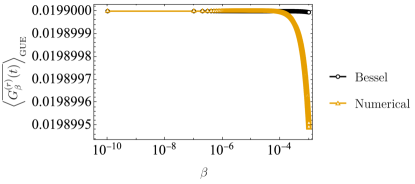
and is independent of . Contrast this, with the equilibration value for nearly maximally entangled Hamiltonians Eq. 42, as computed above. Let us consider Hamiltonians from the Gaussian Unitary Ensemble (GUE) as an example. The eigenstates of these are known to have near maximal entanglement and therefore, we can approximate the . Moreover, for large-, the partition function after ensemble averaging can be expressed as [Mehta(2004), Vijay and Vishwanath(2018)], , where is the modified Bessel function of the first kind. Therefore, the ensemble averaged equilibration value of for the GUE is 111We have implicitly assumed here that the ensemble averaging and the large- limits commute, see [Cotler et al.(2017a)Cotler, Hunter-Jones, Liu, and Yoshida, Xu et al.(2021)Xu, Chenu, Prosen, and del Campo] for a discussion.
| (46) |
Notice that, . Therefore, we can extract from this, both the low- and high-temperature estimates. In Fig. 1 we plot the Bessel function form along with the numerical estimate of the long-time average of the connected BROTOC for the GUE, obtained by averaging (numerically generated) GUE Hamiltonians for .
NRC-product states (NRC-PS).— We introduce a Hamiltonian model that has a generic spectrum, namely, one that satisfies NRC but with all eigenstates as product states (for example, the computational basis states), that we call “NRC-PS”. The Hamiltonian can be expressed as,
| (47) |
where the spectrum satisfies NRC222Note that any Hamiltonian that satisfies NRC cannot be noninteracting, i.e., cannot be of the form since such a Hamiltonian would, by construction, violate NRC. As an example, consider product eigenstates of the form, then it is easy to find pairs of eigenstates for which the energy gaps are equal [Short(2011)]. However, the converse is not true, namely, there exist interacting Hamiltonians, i.e., of the form that have product eigenstates.; for example, consider the spectrum of a Hamiltonian from a Gaussian Unitary Ensemble (GUE). The reason to introduce such a model is twofold: first, it allows us to disentangle the spectral and eigenstate contributions to the equilibration value since, it has the spectrum of a “chaotic” model and the eigenstate properties of a “free” model. Second, as we show now, this model is analytically tractable. The key reason for this is that the NRC-PS model has an extensive number of conserved quantities, of them in fact. A local operator of the form, commutes with the Hamiltonian above, . Similarly, operators of the form, also commute with the Hamiltonian, . Therefore, the Hamiltonian has number of local conserved quantities. In this sense, this is an integrable model, notice however, that its spectrum is intentionally chosen to satisfy NRC.
The presence of conserved quantities enable an exact calculation for the equilibration value of the BROTOC in this model. A detailed proof of this can be found in the Appendix.
| (48) |
where the probability vector is as in the above and are its marginals e.g.,
4 Numerical simulations
In this section we study numerically various dynamical features of the
BROTOC. In particular, we vary the degree
of integrability of Hamiltonian systems and quantify it’s effect on
the equilibration value . At
, this is equal to one minus the operator entanglement of
the dynamical unitary, whose equilibration value was used to
distinguish various integrable and chaotic models in
Ref. [Styliaris et al.(2021)Styliaris, Anand, and Zanardi], see also Refs. [Zhou and Luitz(2017), García-Mata et al.(2018)García-Mata, Saraceno, Jalabert,
Roncaglia, and Wisniacki, Fortes et al.(2019)Fortes,
García-Mata, Jalabert, and Wisniacki, Fortes et al.(2020)Fortes,
García-Mata, Jalabert, and Wisniacki] for distinguishing integrable and chaotic models via time-averages of the OTOC or operator entanglement. We also refer the reader to Ref. [Balachandran et al.(2021)Balachandran, Benenti, Casati, and Poletti], where bounds on decay of OTOCs in time were obtained using the scaling of the time-averaged OTOC. Here, we perform more
extensive numerical studies, consider more generally the -dependence of this quantity, and focus
on the following Hamiltonian models of interest:
-
1.
Integrable model: The transverse-field Ising model (TFIM) with the Hamiltonian, as a paradigmatic quantum spin-chain model. Here, the are the Pauli matrices. For the TFIM, denotes the strength of the transverse field and the local field, respectively. The TFIM Hamiltonian is integrable for either or and nonintegrable when both are nonzero. We consider as the integrable point, and the nonintegrable point . At the integrable point, this model can be mapped onto free fermions via the Jordan-Wigner transformation and is “highly integrable” in this sense. At the nonintegrable point, the model is quantum chaotic, in the sense of random matrix spectral statistics [Bañuls et al.(2011)Bañuls, Cirac, and Hastings, Kim and Huse(2013)] and volume-law entanglement of eigenstates [Wolf et al.(2008)Wolf, Verstraete, Hastings, and Cirac].
-
2.
Localized models: We study Anderson and many-body localization (MBL) with the Hamiltonian, where we draw from the uniform distribution, each . In the absence of the longitudinal field, i.e., , and for nonzero disorder, this (disordered) free fermion model is Anderson localized. In the presence of the longitudinal field, the fermions are interacting and at sufficiently strong disoder, the model is many-body localized (MBL). As is well-known, MBL escapes thermalization by emergent integrability [Nandkishore and Huse(2015), D’Alessio et al.(2016)D’Alessio, Kafri, Polkovnikov, and Rigol]. We refer the reader to Ref. [Chen et al.(2017)Chen, Zhou, Huse, and Fradkin] for a discussion of the long-time values of the unregularized OTOC in localized phases. In our numerical simulations, we focus on for the disorder strength and for the MBL case. We average each instance of the disordered model over independent realizations. In each case, the error bars are too small to plot alongside the data points.
-
3.
NRC-product states (NRC-PS): As introduced before this model allows us to separate the spectral and eigenstate contributions to the BROTOC’s equilibration value. We choose a “chaotic” spectrum (in the sense that it corresponds to a GUE Hamiltonian and hence is an instance of a model that obeys Wigner-Dyson statistics), while having the eigenstates of a noninteracting model, that is, simple product states. To study the NRC-PS model numerically, we generate a random matrix from the Gaussian Unitary Ensemble (GUE) and use its spectrum, while keeping product eigenstates. We average this numerically over independent realizations. This yields numerical results consistent with the analytical expression obtained from Eq. 48.
-
4.
Random matrices: As a benchmark for a “maximally chaotic” model, we consider Hamiltonians drawn from the GUE. For Hamiltonian systems, the seminal works of Berry and Tabor [Berry and Tabor(1977)] and that of Bohigas, Giannoni, and Schmit [Bohigas et al.(1984)Bohigas, Giannoni, and Schmit] establishes that Poisson level-statistics is a characteristic feature of integrable, while for thermalizing systems, Wigner-Dyson statistics are the norm [Rigol et al.(2008)Rigol, Dunjko, and Olshanii, Nandkishore and Huse(2015)]. Furthermore, the eigenstates of GUE are nearly maximally entangled and will provide an analytically tractable example of a highly chaotic model. For our numerical simulations, we generate random matrices and average over independent realizations. The error bars are too small to plot alongside the data points in this case as well. The “ME” in the plots corresponds to a maximally entangled model for which we use the analytical expressions from Eq. 40. For this we generate the spectrum from the GUE and average over independent realizations.
Throughout this section, to evaluate the time-averages numerically, we use two different methods. First, for the Anderson and TFIM integrable model, since it does not satisfy NRC (the Hamiltonian has symmetries), we perform exact time evolution. We do this for a time interval of with a time steps in between. This is fixed for all the system sizes and inverse temperatures . All models except these two satisfy NRC (also verified numerically) and so we compute using the analytical expression in 4. To do this, we perform exact diagonalization of the full Hamiltonian for this and compute the reduced states. At large , it is easy to show that one only needs the ground state along with a few excited states to estimate the time-average in 4. Therefore, for and , we only extract the lowest Hamiltonian eigenstates.
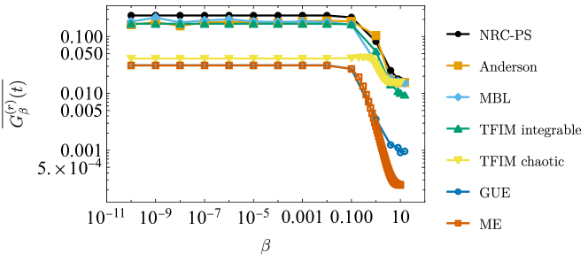
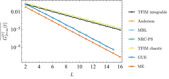
The first numerical result focusses on qubits and we study the variation of as a function of . In Fig. 2, we notice the following universal features of as a function of : the equilibration value is very slowly decaying as varies from zero to . Around , the equilibration value quickly decays to the asymptotic value. Using, 3, we note that the asymptotic value is proportional to the operator purity for the ground state projector. With these universal features at hand, we systematically study the equilibration value for three representative choices of : and . We numerically study their scaling as a function of the system size for a symmetric bipartition of the lattice, . For the case where is not even, the numerical results are very similar for either choice of bipartition, or , and therefore, we choose the former throughout. We also label as “logplot” a plot with logarithmic scale on the -axis and “loglogplot” those with logarithmic scale on both - and -axes.
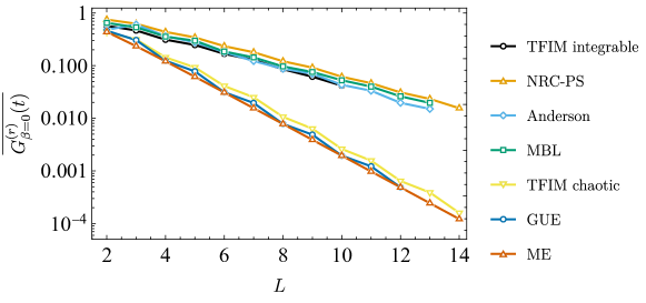
The results for are discussed in Fig. 3. We notice that the scaling w.r.t. the system size is effectively divided into two classes: the quantum chaotic models, namely, the nonintegrable TFIM and the GUE. And, the second class is all the others, namely, the free fermions, the Anderson and MBL, and the NRC-PS. These two classes are primarily distinguished by their eigenstate entanglement, namely, the scaling of the entanglement across the entire spectrum. This, perhaps, comes as no surprise since the infinite-temperature OTOC by construction probes the entanglement across all eigenstates.
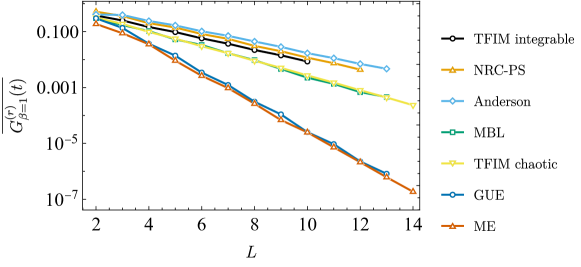
At , from Fig. 4, we notice that the MBL and quantum chaotic models have merged, while having a distinct scaling from the other integrable models and the GUE. Recall that at , Theorem 6 of Ref. [Styliaris et al.(2021)Styliaris, Anand, and Zanardi] establishes a hierarchy between the equilibration values of various estimates for the equlibration value. However, for the regularized OTOC, this result does not necessarily hold away from the case since now we have extra -dependent terms in the NRC estimate; see 3.
And finally, the scaling for can be understood using 3. For the nondegenerate Hamiltonians, this simply probes the ground state entanglement. We notice that all curves coalesce into two groups, one for the integrable/localized models and the second for the GUE and ME models, respectively. While these models vary in their degree of integrability, their ground states (apart from the GUE/ME) all follow an area law [Wolf et al.(2008)Wolf, Verstraete, Hastings, and Cirac] and hence obey a different decay rate with from the GUE. Note that the GUE ground state is a Haar random state and therefore, should scale as , which is consistent with the finite-size scaling results.
| Model | |||
|---|---|---|---|
| TFIM integrable | 0.507672 | 0.687979 | 1.01858 |
| NRC-PS | 0.495827 | 0.7218 | 1.00 |
| Anderson | 0.557617 | 0.655576 | 1.00 |
| MBL | 0.491745 | 0.883465 | 1.00075 |
| TFIM chaotic | 1.00781 | 0.884371 | 0.999999 |
| GUE | 0.999992 | 1.76251 | 2.00016 |
Finite-size scaling.— To quantitatively understand the numerical results, we perform finite-size scaling analysis for each choice of . Let us start with the infinite-temperature case (). We consider an Ansatz of the form,
| (49) |
where is the Hilbert space dimension and is the asymptotic value, i.e., as . From several analytical and numerical results, we know that . That is, the BROTOC decays for all models, free, integrable, or chaotic. Therefore, we reduce the Ansatz to
| (50) |
As a result, we have, where . The numerical results naturally manifest this Ansatz as is evident from the nearly linear figures. Therefore, performing a linear fit to the versus plots yields the decay rates corresponding to various models. We focus on the last 5 data points to obtain the fit parameters, see the Appendix for more details.
The finite-size scaling results are summarized in Table 1. The decay rates are universal at with for the integrable models and for the chaotic models. Around , this universality begins to breakdown and at large , the equilibration value only differentiates local models from the nonlocal GUE model.
From the analytical results about NRC-PS and GUE, we know that at , the . And, from the finite-size scaling results, we obtain, . At , using 3, for both NRC-PS and GUE, the equilibration value is determined by the ground state purity. Therefore, for NRC-PS, it scales as and for GUE it scales as since GUE ground states are Haar-random states, their purity is near minimum, with corrections, which is also consistent with the finite-size scaling results. Therefore, the ratio of the rates in this case is also . And finally, from the numerical values listed in Table 1, we see that the ratio is at as well.
5 Conclusions
In this work we introduce the bipartite regularized OTOC that allows us to obtain a wealth of analytical and numerical results to aid our understanding of regularized OTOCs for local quantum systems. The infinite-temperature OTOC has several operational interpretations in terms of operator entanglement, entropy production, and others. Proposition 1 established the connected component of the BROTOC as probing the operator purity of a quantum operation. We then showed that the quantum operation is intimately related to the two-point spectral form factor and globally averaged regularized OTOCs are connected to the four-point spectral form factor, respectively. Moreover, the connected BROTOC probes the purity of the associated thermofield double state.
Moving away from the infinite-temperature assumption, we investigate the zero-temperature case, where, in Proposition 3, we showed that, in this limit, both the disconnected and connected components of the BROTOC probe the groundstate entanglement for nondegenerate Hamiltonians. This allows us to think of them as probes to quantum phase transitions in the system.
In Propositions 4 and 5, we study the equilibration value of the BROTOC and how it connects to eigenstate entanglement. In fact, we show that if there is sufficient entanglement in all eigenstates across the spectrum, then the equilibration value must be nearly maximal. We also obtain analytical closed-form expressions for the equilibration value of nearly maximally-entangled Hamiltonians and contrast the -dependence in the unregularized versus the regularized case.
Finally, we perform numerical simulations on various integrable and
chaotic Hamiltonian models to study the equilibration value of the
connected component of the BROTOC. Using a mix of finite-size scaling
and analytical estimates, we contrast the decay rates of the BROTOC
for various models. While at , the decay rate is
universal and distinguishes integrable, chaotic, and random matrix
evolutions; as we reach , this universality begins to
break down. And, in fact, at , the
equilibration value only distinguishes local models from the GUE, and
is therefore no longer a reliable signature of chaotic-vs-integrable
dynamics. An interesting future work would be to contrast various
choices of regularizations and their ability to distinguish chaotic
and integrable dynamics.
6 Acknowledgments
N.A. would like to thank G. Styliaris for many insightful discussions. The authors acknowledge the Center for Advanced Research Computing (CARC) at the University of Southern California for providing computing resources that have contributed to the research results reported within this publication. URL: https://carc.usc.edu. The authors acknowledge partial support from the NSF award PHY-1819189. This research was (partially) sponsored by the Army Research Office and was accomplished under Grant Number W911NF-20-1-0075. The views and conclusions contained in this document are those of the authors and should not be interpreted as representing the official policies, either expressed or implied, of the Army Research Office or the U.S. Government. The U.S. Government is authorized to reproduce and distribute reprints for Government purposes notwithstanding any copyright notation herein.
References
- [Srednicki(1994)] M. Srednicki, Physical Review E 50, 888 (1994).
- [Rigol et al.(2008)Rigol, Dunjko, and Olshanii] M. Rigol, V. Dunjko, and M. Olshanii, Nature 452, 854 (2008).
- [D’Alessio et al.(2016)D’Alessio, Kafri, Polkovnikov, and Rigol] L. D’Alessio, Y. Kafri, A. Polkovnikov, and M. Rigol, Advances in Physics 65, 239 (2016).
- [Borgonovi et al.(2016)Borgonovi, Izrailev, Santos, and Zelevinsky] F. Borgonovi, F. Izrailev, L. Santos, and V. Zelevinsky, Physics Reports 626, 1 (2016).
- [von Keyserlingk et al.(2018)von Keyserlingk, Rakovszky, Pollmann, and Sondhi] C. W. von Keyserlingk, T. Rakovszky, F. Pollmann, and S. L. Sondhi, Phys. Rev. X 8, 021013 (2018).
- [Nahum et al.(2018)Nahum, Vijay, and Haah] A. Nahum, S. Vijay, and J. Haah, Phys. Rev. X 8, 021014 (2018).
- [Rakovszky et al.(2018)Rakovszky, Pollmann, and von Keyserlingk] T. Rakovszky, F. Pollmann, and C. W. von Keyserlingk, Phys. Rev. X 8, 031058 (2018).
- [Khemani et al.(2018a)Khemani, Vishwanath, and Huse] V. Khemani, A. Vishwanath, and D. A. Huse, Phys. Rev. X 8, 031057 (2018a).
- [Gopalakrishnan et al.(2018)Gopalakrishnan, Huse, Khemani, and Vasseur] S. Gopalakrishnan, D. A. Huse, V. Khemani, and R. Vasseur, Phys. Rev. B 98, 220303 (2018).
- [Chan et al.(2018)Chan, De Luca, and Chalker] A. Chan, A. De Luca, and J. T. Chalker, Phys. Rev. X 8, 041019 (2018).
- [Parker et al.(2019)Parker, Cao, Avdoshkin, Scaffidi, and Altman] D. E. Parker, X. Cao, A. Avdoshkin, T. Scaffidi, and E. Altman, Physical Review X 9, 041017 (2019).
- [Murthy and Srednicki(2019)] C. Murthy and M. Srednicki, Physical Review Letters 123, 230606 (2019).
- [Maldacena et al.(2016)Maldacena, Shenker, and Stanford] J. Maldacena, S. H. Shenker, and D. Stanford, Journal of High Energy Physics 2016, 1 (2016).
- [Xu et al.(2020)Xu, Scaffidi, and Cao] T. Xu, T. Scaffidi, and X. Cao, Phys. Rev. Lett. 124, 140602 (2020).
- [Swingle(2018)] B. Swingle, Nature Physics 14, 988 (2018).
- [Xu and Swingle(2022)] S. Xu and B. Swingle, arXiv:2202.07060 (2022).
- [Larkin and Ovchinnikov(1969)] I. A. Larkin and Y. N. Ovchinnikov, Journal of Experimental and Theoretical Physics 28, 2262 (1969).
- [Kitaev(2015)] A. Kitaev, “A simple model of quantum holography (part 1),” http://online.kitp.ucsb.edu/online/entangled15/kitaev/ (2015).
- [Lieb and Robinson(1972)] E. H. Lieb and D. W. Robinson, in Statistical mechanics (Springer, 1972) pp. 425–431.
- [Hastings and Koma(2006)] M. B. Hastings and T. Koma, Communications in Mathematical Physics 265, 781 (2006).
- [Bravyi et al.(2006)Bravyi, Hastings, and Verstraete] S. Bravyi, M. B. Hastings, and F. Verstraete, Physical Review Letters 97, 050401 (2006).
- [Cotler et al.(2017a)Cotler, Hunter-Jones, Liu, and Yoshida] J. Cotler, N. Hunter-Jones, J. Liu, and B. Yoshida, J. High Energ. Phys. 2017, 48 (2017a).
- [Hosur et al.(2016)Hosur, Qi, Roberts, and Yoshida] P. Hosur, X.-L. Qi, D. A. Roberts, and B. Yoshida, Journal of High Energy Physics 2016, 1 (2016).
- [Mi et al.(2021)Mi, Roushan, Quintana, Mandra, Marshall, Neill, Arute, Arya, Atalaya, Babbush et al.] X. Mi, P. Roushan, C. Quintana, S. Mandra, J. Marshall, C. Neill, F. Arute, K. Arya, J. Atalaya, R. Babbush, et al., Science 374, 1479 (2021).
- [Braumüller et al.(2022)Braumüller, Karamlou, Yanay, Kannan, Kim, Kjaergaard, Melville, Niedzielski, Sung, Vepsäläinen et al.] J. Braumüller, A. H. Karamlou, Y. Yanay, B. Kannan, D. Kim, M. Kjaergaard, A. Melville, B. M. Niedzielski, Y. Sung, A. Vepsäläinen, et al., Nature Physics 18, 172 (2022).
- [Wei et al.(2018)Wei, Ramanathan, and Cappellaro] K. X. Wei, C. Ramanathan, and P. Cappellaro, Phys. Rev. Lett. 120, 070501 (2018).
- [Li et al.(2017)Li, Fan, Wang, Ye, Zeng, Zhai, Peng, and Du] J. Li, R. Fan, H. Wang, B. Ye, B. Zeng, H. Zhai, X. Peng, and J. Du, Physical Review X 7, 031011 (2017).
- [Nie et al.(2019)Nie, Zhang, Zhao, Xin, Lu, and Li] X. Nie, Z. Zhang, X. Zhao, T. Xin, D. Lu, and J. Li, arXiv:1903.12237 (2019).
- [Nie et al.(2020)Nie, Wei, Chen, Zhang, Zhao, Qiu, Tian, Ji, Xin, Lu, and Li] X. Nie, B.-B. Wei, X. Chen, Z. Zhang, X. Zhao, C. Qiu, Y. Tian, Y. Ji, T. Xin, D. Lu, and J. Li, Phys. Rev. Lett. 124, 250601 (2020).
- [Gärttner et al.(2017)Gärttner, Bohnet, Safavi-Naini, Wall, Bollinger, and Rey] M. Gärttner, J. G. Bohnet, A. Safavi-Naini, M. L. Wall, J. J. Bollinger, and A. M. Rey, Nature Physics 13, 781 (2017).
- [Joshi et al.(2020)Joshi, Elben, Vermersch, Brydges, Maier, Zoller, Blatt, and Roos] M. K. Joshi, A. Elben, B. Vermersch, T. Brydges, C. Maier, P. Zoller, R. Blatt, and C. F. Roos, Phys. Rev. Lett. 124, 240505 (2020).
- [Meier et al.(2019)Meier, Ang’ong’a, An, and Gadway] E. J. Meier, J. Ang’ong’a, F. A. An, and B. Gadway, Phys. Rev. A 100, 013623 (2019).
- [Chen et al.(2020)Chen, Hou, Zhou, Qian, Shen, and Xu] B. Chen, X. Hou, F. Zhou, P. Qian, H. Shen, and N. Xu, Applied Physics Letters 116, 194002 (2020).
- [Yan et al.(2020)Yan, Cincio, and Zurek] B. Yan, L. Cincio, and W. H. Zurek, Phys. Rev. Lett. 124, 160603 (2020).
- [Styliaris et al.(2021)Styliaris, Anand, and Zanardi] G. Styliaris, N. Anand, and P. Zanardi, Physical Review Letters 126, 030601 (2021).
- [Zanardi and Anand(2021)] P. Zanardi and N. Anand, Physical Review A 103, 062214 (2021).
- [Anand et al.(2021)Anand, Styliaris, Kumari, and Zanardi] N. Anand, G. Styliaris, M. Kumari, and P. Zanardi, Phys. Rev. Research 3, 023214 (2021).
- [Yunger Halpern et al.(2019)Yunger Halpern, Bartolotta, and Pollack] N. Yunger Halpern, A. Bartolotta, and J. Pollack, Commun Phys 2, 92 (2019).
- [Zanardi(2001)] P. Zanardi, Phys. Rev. A 63, 040304 (2001).
- [Wang and Zanardi(2002)] X. Wang and P. Zanardi, Phys. Rev. A 66, 044303 (2002).
- [Zanardi et al.(2000)Zanardi, Zalka, and Faoro] P. Zanardi, C. Zalka, and L. Faoro, Phys. Rev. A 62, 030301 (2000).
- [Touil and Deffner(2021)] A. Touil and S. Deffner, PRX Quantum 2, 010306 (2021).
- [Watrous(2018)] J. Watrous, The Theory of Quantum Information, 1st ed. (Cambridge University Press, 2018).
- [Tsuji et al.(2018)Tsuji, Shitara, and Ueda] N. Tsuji, T. Shitara, and M. Ueda, Physical Review E 98, 012216 (2018).
- [Foini and Kurchan(2019)] L. Foini and J. Kurchan, Physical Review E 99, 042139 (2019).
- [Vijay and Vishwanath(2018)] S. Vijay and A. Vishwanath, arXiv:1803.08483 (2018).
- [Sahu and Swingle(2020)] S. Sahu and B. Swingle, Physical Review B 102, 184303 (2020).
- [Liao and Galitski(2018)] Y. Liao and V. Galitski, Phys. Rev. B 98, 205124 (2018).
- [Nielsen and Chuang(2010)] M. A. Nielsen and I. L. Chuang, Quantum Computation and Quantum Information, 10th ed. (Cambridge University Press, Cambridge ; New York, 2010).
- [Plenio and Virmani(2005)] M. B. Plenio and S. Virmani, arXiv:quant-ph/0504163 (2005).
- [Lupo et al.(2008)Lupo, Aniello, and Scardicchio] C. Lupo, P. Aniello, and A. Scardicchio, Journal of Physics A: Mathematical and Theoretical 41, 415301 (2008).
- [Aniello and Lupo(2009)] P. Aniello and C. Lupo, Open Systems and Information Dynamics 16, 127–143 (2009).
- [Zhou and Luitz(2017)] T. Zhou and D. J. Luitz, Phys. Rev. B 95, 094206 (2017).
- [Kukuljan et al.(2017)Kukuljan, Grozdanov, and Prosen] I. Kukuljan, S. Grozdanov, and T. Prosen, Phys. Rev. B 96, 060301 (2017).
- [Lin and Motrunich(2018)] C.-J. Lin and O. I. Motrunich, Phys. Rev. B 97, 144304 (2018).
- [Chen and Zhou(2019)] X. Chen and T. Zhou, Phys. Rev. B 100, 064305 (2019).
- [Khemani et al.(2018b)Khemani, Huse, and Nahum] V. Khemani, D. A. Huse, and A. Nahum, Phys. Rev. B 98, 144304 (2018b).
- [Chen(2016)] Y. Chen, arXiv:1608.02765 (2016).
- [Avdoshkin and Dymarsky(2020)] A. Avdoshkin and A. Dymarsky, Phys. Rev. Research 2, 043234 (2020).
- [Haake(2010)] F. Haake, Quantum Signatures of Chaos, 3rd ed., Springer Series in Synergetics No. 54 (Springer, Berlin ; New York, 2010).
- [Guhr et al.(1998)Guhr, Müller–Groeling, and Weidenmüller] T. Guhr, A. Müller–Groeling, and H. A. Weidenmüller, Physics Reports 299, 189 (1998).
- [Mehta(2004)] M. L. Mehta, Random Matrices, 3rd ed., Pure and Applied Mathematics Series No. 142 (Elsevier, Amsterdam, 2004).
- [Berry(1985)] M. V. Berry, Proc. R. Soc. Lond. A 400, 229 (1985).
- [Takahashi and Umezawa(1996)] Y. Takahashi and H. Umezawa, International Journal of Modern Physics B 10, 1755 (1996).
- [Dyer and Gur-Ari(2017)] E. Dyer and G. Gur-Ari, J. High Energ. Phys. 2017, 75 (2017).
- [del Campo et al.(2017)del Campo, Molina-Vilaplana, and Sonner] A. del Campo, J. Molina-Vilaplana, and J. Sonner, Physical Review D 95, 126008 (2017).
- [Papadodimas and Raju(2015)] K. Papadodimas and S. Raju, Phys. Rev. Lett. 115, 211601 (2015).
- [Wu and Hsieh(2019)] J. Wu and T. H. Hsieh, Phys. Rev. Lett. 123, 220502 (2019).
- [Martyn and Swingle(2019)] J. Martyn and B. Swingle, Phys. Rev. A 100, 032107 (2019).
- [Zhu et al.(2020)Zhu, Johri, Linke, Landsman, Huerta Alderete, Nguyen, Matsuura, Hsieh, and Monroe] D. Zhu, S. Johri, N. M. Linke, K. A. Landsman, C. Huerta Alderete, N. H. Nguyen, A. Y. Matsuura, T. H. Hsieh, and C. Monroe, Proc. Natl. Acad. Sci. U.S.A. 117, 25402 (2020).
- [Cottrell et al.(2019)Cottrell, Freivogel, Hofman, and Lokhande] W. Cottrell, B. Freivogel, D. M. Hofman, and S. F. Lokhande, J. High Energ. Phys. 2019, 58 (2019).
- [Lantagne-Hurtubise et al.(2020)Lantagne-Hurtubise, Plugge, Can, and Franz] E. Lantagne-Hurtubise, S. Plugge, O. Can, and M. Franz, Phys. Rev. Research 2, 013254 (2020).
- [Cotler et al.(2017b)Cotler, Hunter-Jones, Liu, and Yoshida] J. Cotler, N. Hunter-Jones, J. Liu, and B. Yoshida, Journal of High Energy Physics 2017 (2017b), 10.1007/JHEP11(2017)048.
- [Wilde(2016)] M. M. Wilde, From Classical to Quantum Shannon Theory, cambridge university press ed. (2016).
- [Sekino and Susskind(2008)] Y. Sekino and L. Susskind, Journal of High Energy Physics 2008, 065–065 (2008).
- [Lashkari et al.(2013)Lashkari, Stanford, Hastings, Osborne, and Hayden] N. Lashkari, D. Stanford, M. Hastings, T. Osborne, and P. Hayden, J. High Energ. Phys. 2013, 22 (2013).
- [Sá et al.(2020a)Sá, Ribeiro, and Prosen] L. Sá, P. Ribeiro, and T. Prosen, Journal of Physics A: Mathematical and Theoretical 53, 305303 (2020a).
- [Denisov et al.(2019)Denisov, Laptyeva, Tarnowski, Chruściński, and Życzkowski] S. Denisov, T. Laptyeva, W. Tarnowski, D. Chruściński, and K. Życzkowski, Phys. Rev. Lett. 123, 140403 (2019).
- [Can(2019)] T. Can, Journal of Physics A: Mathematical and Theoretical 52, 485302 (2019).
- [Can et al.(2019)Can, Oganesyan, Orgad, and Gopalakrishnan] T. Can, V. Oganesyan, D. Orgad, and S. Gopalakrishnan, Phys. Rev. Lett. 123, 234103 (2019).
- [Grobe et al.(1988)Grobe, Haake, and Sommers] R. Grobe, F. Haake, and H.-J. Sommers, Phys. Rev. Lett. 61, 1899 (1988).
- [Akemann et al.(2019)Akemann, Kieburg, Mielke, and Prosen] G. Akemann, M. Kieburg, A. Mielke, and T. c. v. Prosen, Phys. Rev. Lett. 123, 254101 (2019).
- [Sá et al.(2020b)Sá, Ribeiro, and Prosen] L. Sá, P. Ribeiro, and T. Prosen, Physical Review X 10, 021019 (2020b).
- [Zurek and Paz(1994)] W. H. Zurek and J. P. Paz, Physical Review Letters 72, 2508 (1994).
- [Sachdev(2011)] S. Sachdev, Quantum Phase Transitions, second edition ed. (Cambridge University Press, Cambridge ; New York, 2011).
- [Heyl et al.(2018)Heyl, Pollmann, and Dóra] M. Heyl, F. Pollmann, and B. Dóra, Phys. Rev. Lett. 121, 016801 (2018).
- [Reimann(2008)] P. Reimann, Phys. Rev. Lett. 101, 190403 (2008).
- [Linden et al.(2009)Linden, Popescu, Short, and Winter] N. Linden, S. Popescu, A. J. Short, and A. Winter, Phys. Rev. E 79, 061103 (2009).
- [Campos Venuti et al.(2011)Campos Venuti, Jacobson, Santra, and Zanardi] L. Campos Venuti, N. T. Jacobson, S. Santra, and P. Zanardi, Phys. Rev. Lett. 107, 010403 (2011).
- [Alhambra et al.(2020)Alhambra, Riddell, and García-Pintos] A. M. Alhambra, J. Riddell, and L. P. García-Pintos, Phys. Rev. Lett. 124, 110605 (2020).
- [García-Mata et al.(2018)García-Mata, Saraceno, Jalabert, Roncaglia, and Wisniacki] I. García-Mata, M. Saraceno, R. A. Jalabert, A. J. Roncaglia, and D. A. Wisniacki, Phys. Rev. Lett. 121, 210601 (2018).
- [Fortes et al.(2019)Fortes, García-Mata, Jalabert, and Wisniacki] E. M. Fortes, I. García-Mata, R. A. Jalabert, and D. A. Wisniacki, Phys. Rev. E 100, 042201 (2019).
- [Huang et al.(2019)Huang, Brandão, and Zhang] Y. Huang, F. G. S. L. Brandão, and Y.-L. Zhang, Phys. Rev. Lett. 123, 010601 (2019).
- [Short(2011)] A. J. Short, New Journal of Physics 13, 053009 (2011).
- [Xu et al.(2021)Xu, Chenu, Prosen, and del Campo] Z. Xu, A. Chenu, T. Prosen, and A. del Campo, Phys. Rev. B 103, 064309 (2021).
- [Fortes et al.(2020)Fortes, García-Mata, Jalabert, and Wisniacki] E. M. Fortes, I. García-Mata, R. A. Jalabert, and D. A. Wisniacki, EPL (Europhysics Letters) 130, 60001 (2020).
- [Balachandran et al.(2021)Balachandran, Benenti, Casati, and Poletti] V. Balachandran, G. Benenti, G. Casati, and D. Poletti, Phys. Rev. B 104, 104306 (2021).
- [Bañuls et al.(2011)Bañuls, Cirac, and Hastings] M. C. Bañuls, J. I. Cirac, and M. B. Hastings, Phys. Rev. Lett. 106, 050405 (2011).
- [Kim and Huse(2013)] H. Kim and D. A. Huse, Phys. Rev. Lett. 111, 127205 (2013).
- [Wolf et al.(2008)Wolf, Verstraete, Hastings, and Cirac] M. M. Wolf, F. Verstraete, M. B. Hastings, and J. I. Cirac, Phys. Rev. Lett. 100, 070502 (2008).
- [Nandkishore and Huse(2015)] R. Nandkishore and D. A. Huse, Annual Review of Condensed Matter Physics 6, 15 (2015).
- [Chen et al.(2017)Chen, Zhou, Huse, and Fradkin] X. Chen, T. Zhou, D. A. Huse, and E. Fradkin, Annalen der Physik 529, 1600332 (2017).
- [Berry and Tabor(1977)] M. V. Berry and M. Tabor, Proc. R. Soc. Lond. A 356, 375 (1977).
- [Bohigas et al.(1984)Bohigas, Giannoni, and Schmit] O. Bohigas, M. J. Giannoni, and C. Schmit, Physical Review Letters 52, 1 (1984).
- [Pollock et al.(2018a)Pollock, Rodríguez-Rosario, Frauenheim, Paternostro, and Modi] F. A. Pollock, C. Rodríguez-Rosario, T. Frauenheim, M. Paternostro, and K. Modi, Phys. Rev. A 97, 012127 (2018a).
- [Pollock et al.(2018b)Pollock, Rodríguez-Rosario, Frauenheim, Paternostro, and Modi] F. A. Pollock, C. Rodríguez-Rosario, T. Frauenheim, M. Paternostro, and K. Modi, Phys. Rev. Lett. 120, 040405 (2018b).
Appendices
Proof of 1
See 1
Consider a bipartite Hilbert space, . Let and denote the Haar average of over . Then, using the lemma [Watrous(2018)],
| (A1) |
where is the swap operator on with representing a replica of the original Hilbert space . Given an orthonormal basis of , (and a replica of the basis for ), the swap operator can be represented as . Now, if we consider Haar averages over a subsystem instead, then the lemma above is modified as,
| (A2) |
First, we compute the disconnected BROTOC,
| (A3) | ||||
| (A4) | ||||
| (A5) |
where in the second line, we have used the lemma, and in the third line we have used , , , and .
We can formally perform partial traces above, for example,
| (A6) |
where above for brevity. Let be the squared -norm of the operator with and with the complement of . Then,
| (A7) |
Similarly, for the connected BROTOC we have,
| (A8) | ||||
| (A9) | ||||
| (A10) | ||||
| (A11) |
where with the imaginary time-evolution, the real time-evolution, and the usual time-evolution operator. This completes the proof.
Proof of 4
See 4
Recall that NRC implies nondegeneracy of the spectrum, therefore, using the spectral decomposition of a Hamiltonian, with , we have,
| (A12) |
Using the NRC assumption, we have the following, . Therefore,
| (A13) | ||||
| (A14) | ||||
| (A15) |
Now, for pure states one can show that .
We now define the -matrix introduced in Ref. [Styliaris et al.(2021)Styliaris, Anand, and Zanardi] while computing the infinite-temperature variant of this Proposition. Let be the reduced state, then, formally performing the partial trace we have,
| (A16) |
Therefore, the time-average can be simplified as,
| (A17) |
Now we introduce a more compact notation for the equilibration value. Let , then,
| (A18) |
with ; where we have used the fact that , that is, the the reduced states and are isospectral (up to irrelevant zeros).
Proof of 5
See 5
We prove this for the general case , and the original Proposition can be recovered by setting at the end. Let us assume without loss of generality that . The spectral decomposition of the Hamiltonian is and its reduced states are labelled as .
Notice that since , the assumption that the purities are nearly minimum can be equivalently expressed as: with .
Define analogously, i.e., . Then, using the fact that the reduced states of a pure state are isospectral (therefore, ) and , we have, .
Now, recall that, and , where we have used the fact that . Then,
| (A19) | |||
| (A20) |
where we have split the terms in and then used the triangle inequality. We now want to bound each of the terms .
Since (note that we do not need an absolute value here since the exponential term is nonnegative and so the inner products between the reduced states is nonnegative as well); we need to bound . Note that,
| (A21) |
And, using Cauchy-Schwarz inequality along with the fact that (as shown above), we have, . Therefore, .
Plugging this back in , we have, . Now, for the diagonal part, .
Therefore, term above becomes and term becomes, . And, term becomes, . Now, notice that
| (A22) | ||||
| (A23) |
where we have dropped the terms in the summation and used their nonnegativity. Therefore, and so, term (iii) can be upper bounded as .
Putting everything together, we have
| (A24) |
Now, if we set , we have, . Therefore,
| (A25) |
Proof of 2
See 2
We have,
| (A26) |
where we have used . Now, using the cyclicity of trace and the lemma , we have,
| (A27) | ||||
| (A28) |
where in the second line we have used the cyclicity of trace to move to the front. Now, performing using the lemma above, we have,
| (A29) |
Similarly, performing the average over we obtain the final terms that are proportional to . Thus, we have the desired result.
Unregularized OTOCs for maximally entangled models
Consider an operator Schmidt decomposition of with and such that and . Forr a unitary operator, , therefore, we have,
| (A30) |
Now, consider the bipartite unregularized OTOC, . Plugging in the operator Schmidt decomposition of , we have,
where we have used the adjoint action . Then,
| (A31) |
where we have used the fact that and and summed over two of the indices of the summation above. Now, if is maximally entangled (namely, its eigenstates are maximally entangled) across and one has , then
| (A32) |
Therefore, and is independent of .
The dynamical map is a quantum operation
Recall that the Choi-Jamiolkowski (CJ) isomorphism is an isomorphism between linear maps to matrices . Let be the normalized maximally entangled state in , then,
| (A33) |
A linear map is CP . Computing the CJ matrix corresponding to the linear map , we have,
| (A34) | ||||
| (A35) |
where in the second equality we have used the expansion of the TDS Eq. 19. Now, since is a pure state (or a rank- projector), it is positive semidefinite. Moreover, , therefore, . As a result, is a CP map.
To show that the map is trace-nonincreasing, we have to show that . Namely,
| (A36) | |||
| (A37) | |||
| (A38) | |||
| (A39) |
where in the last line, we have used the definition of positive semidefiniteness. Now, assuming , we have, since if . Notice that, the matrix is subnormalized with . Therefore, the dynamical map, is a CP and trace-nonincreasing linear map, that is, it is a physical quantum operation [Nielsen and Chuang(2010)] and we can think of as a subnormalized density matrix corresponding to a quantum process [Pollock et al.(2018a)Pollock, Rodríguez-Rosario, Frauenheim, Paternostro, and Modi, Pollock et al.(2018b)Pollock, Rodríguez-Rosario, Frauenheim, Paternostro, and Modi].
Equilibration value of NRC-PS
To compute the equilibration value, we need to evaluate the -matrix. Recall that , with the additional assumption that the spectrum satisfies NRC. Define the index with and . Then, , that is for all paired indices and the reduced states are the same. For the -matrix, consider and , we have, . Similarly, we have, and .
We are now ready to evaluate . Notice that
| (A40) | |||
| (A41) |
Defining, , we have, . Similar algebraic manipulations prove the final result,
| (A42) |
This can then be rewritten in the form in the main text, namely,
| (A43) |
where the probability vector is defined by the components and are its marginals.
Moreover, for the disconnected correlator, a similar calculation shows that,
| (A44) |
Numerical details
The value for all linear fits was for all data and hence we do not report the numbers here.
| Model | |||
|---|---|---|---|
| TFIM integrable | 0.523785 | 0.0341617 | -0.525957 |
| NRC-PS | 0.971448 | 0.83213 | 1.00 |
| Anderson | 1.13615 | 0.742852 | |
| MBL | 0.700658 | 0.213039 | -0.012799 |
| TFIM chaotic | 1.60648 | 0.327334 | -0.00502613 |
| GUE | 1.12868 | 2.56073 | 2.10215 |